the Creative Commons Attribution 4.0 License.
the Creative Commons Attribution 4.0 License.
 | 11 Oct 2018
Development and implementation of a new biomass burning emissions injection height scheme (BBEIH v1.0) for the GEOS-Chem model (v9-01-01)
Liye Zhu
Maria Val Martin
Luciana V. Gatti
Ralph Kahn
Arsineh Hecobian
Emily V. Fischer
Biomass burning is a significant source of trace gases and aerosols to the atmosphere, and the evolution of these species depends acutely on where they are injected into the atmosphere. GEOS-Chem is a chemical transport model driven by assimilated meteorological data that is used to probe a variety of scientific questions related to atmospheric composition, including the role of biomass burning. This paper presents the development and implementation of a new global biomass burning emissions injection scheme in the GEOS-Chem model. The new injection scheme is based on monthly gridded Multi-angle Imaging SpectroRadiometer (MISR) global plume-height stereoscopic observations in 2008. To provide specific examples of the impact of the model updates, we compare the output from simulations with and without the new MISR-based injection height scheme to several sets of observations from regions with active fires. Our comparisons with Arctic Research on the Composition of the Troposphere from Aircraft and Satellites (ARCTAS) aircraft observations show that the updated injection height scheme can improve the ability of the model to simulate the vertical distribution of peroxyacetyl nitrate (PAN) and carbon monoxide (CO) over North American boreal regions in summer. We also compare a simulation for October 2010 and 2011 to vertical profiles of CO over the Amazon Basin. When coupled with larger emission factors for CO, a simulation that includes the new injection scheme also better matches selected observations in this region. Finally, the improved injection height improves the simulation of monthly mean surface CO over California during July 2008, a period with large fires.
- Article
(3989 KB) - Full-text XML
-
Supplement
(486 KB) - BibTeX
- EndNote


Properly describing the injection altitude of smoke in the atmosphere is an essential step in predicting the impact of emissions from landscape fires on atmospheric composition (Paugam et al., 2016). Injecting smoke higher in the atmosphere in chemical transport models can extend or reduce the lifetime of trace species, and it can alter the spatial extent of smoke influence in the atmosphere (Freitas et al., 2006). The impact of injection height on smoke dispersion is three-fold: (1) winds in the free troposphere are generally stronger than in the boundary layer – thus when smoke is emitted aloft, defined plumes are sometimes detected thousands of kilometers downwind (e.g., Colarco et al., 2004; Damoah et al., 2004; Forster et al., 2001; Val Martin et al., 2006); (2) removal processes tend to be more efficient in the boundary layer (e.g., Boy et al., 2008); (3) chemical evolution within the plume can be sensitive to injection height because altitude impacts plume temperature, ambient relative humidity, smoke–cloud interactions, and photolysis rates (e.g., Freitas et al., 2006). Given the importance for atmospheric composition and air quality predictions (e.g., Stein et al., 2009), substantial efforts have been made to better understand how injection height varies by ecosystem type and season (e.g., Val Martin et al., 2010; Tosca et al., 2011; Mims et al., 2010), which environmental drivers of injection height are most important (e.g., Kahn et al., 2008; Val Martin et al., 2012), and how best to estimate smoke injection height in models (e.g., Paugam et al., 2016, and references therein) to produce improvements in model simulations of trace constituents (e.g., Gonzi et al., 2015).
GEOS-Chem is a global chemical transport model (CTM) (http://geos-chem.org, last access: 6 October 2018; Bey et al., 2001) that is routinely used to simulate the impacts of biomass burning on atmospheric composition (e.g., Lewis et al., 2013; Leung et al., 2007). GEOS-Chem is driven by GEOS assimilated meteorological data from the NASA Global Modeling and Assimilation Office (GMAO), and it includes a state-of-the-science description of tropospheric oxidant chemistry, necessary for understanding the chemical and dynamical processes controlling the evolution of biomass burning emissions. The public-release version of GEOS-Chem emits all biomass burning emissions into the atmospheric boundary layer. This may be appropriate for some fire types but is likely a source of error for many regions with active biomass burning (e.g., Leung et al., 2007). The main objective of the current paper is to introduce a new global biomass burning injection height scheme for GEOS-Chem based on Multi-angle Imaging SpectroRadiometer (MISR) plume injection height observations from 2008. The MISR instrument was launched into a sun-synchronous, polar orbit aboard the NASA Earth Observing System's Terra satellite in December 1999 and acquires global observations at nine viewing angles in each of four spectral bands about once per week (e.g., Diner et al., 1998). Smoke aerosol injection height is derived from source plumes with discernable features in the MISR views (Kahn et al., 2008).
Though biomass burning impacts atmospheric composition across a suite of temporal and geographic scales, this paper presents model–observation comparisons for specific biomass burning plumes having well-sampled vertical structure. The data available to make such important comparisons are limited. However, this is an important step toward using the model to address broader aspects of atmospheric composition. To the best of our knowledge, this paper represents the first effort at using measured global smoke plume injection heights from MISR as constraints on a CTM. There have been efforts to do this on a regional scale for specific fire seasons (e.g., Chen et al., 2009; Jian and Fu, 2014), but we are unaware of similar global implementations. Val Martin et al. (2012) studied the performance of one of the most advanced physically based plume-rise models. They concluded that given the uncertainties and performance of that approach, empirically derived plume injection heights, such as those we use here, provide better constraints on smoke transport.
Much of the model development presented here was motivated by the persistent challenge CTMs appear to face at accurately simulating peroxyacetyl nitrate (PAN) in the atmosphere (e.g., Emmons et al., 2015). This compound plays a central role in oxidant chemistry, particularly in remote regions (Moxim et al., 1996). However, it has a temperature-dependent lifetime (Singh and Hanst, 1981), and thus its evolution in the atmosphere is particularly sensitive to plume injection height. As a first step toward validating the revised model, we compare the output from a simulation with improved injection heights to multiple sets of observations from regions with active fires, providing examples of cases where injecting a substantial percent of biomass burning emissions in the free troposphere is important for properly simulating PAN as well as carbon monoxide (CO).
2.1 Overview of model development
Figure 1 illustrates the process of implementing an observationally based injection scheme into GEOS-Chem. This section describes the details associated with each step in the process. The new injection scheme is based on MISR plume injection height observations from 2008 (Sect. 2.2). The model configuration is described in Sect. 2.3. We then map the native MISR injection altitude (0–8 km) to emitted percentages of total biomass burning emissions to a GMAO 47-layer reduced vertical grid and a horizontal grid (Sect. 2.4).
2.2 Analysis of MISR plume-height observations
The new injection scheme is developed based on the MISR plume-height stereoscopic observations in 2008 (Val Martin et al., 2018). The MISR data we used are part of the MISR Plume Height Project2, which was derived for the AeroCom multi-model biomass burning experiment. The dataset is publicity available from https://misr.jpl.nasa.gov/getData/accessData/MisrMinxPlumes2/ (last access: 8 October 2018). Briefly, MISR-based injection heights are given by altitude (250 m, from 0 to 8 km above ground level), land cover type, season, and region. Land cover classifications are based on the MODIS Level 3 land cover product MOD12Q1 (Friedl et al., 2010). There are 12 classifications used here: evergreen needleleaf forest, evergreen broad-leaf forest, deciduous needleleaf forest, deciduous broad-leaf forest, mixed forest, closed shrub, open shrub, woody savanna, savanna, grassland, wetland, and cropland. We define seasons as spring (MAM), summer (JJA), fall (SON), and winter (DJF) and considered eight main fire regions (North America, South America, Africa, Europe, boreal Eurasia, South Asia, and Australia).
To convert the MISR-based vertical distribution of smoke injection height, Val Martin et al. (2018) first transformed the MISR vertical distribution percentages from 0 to 8 km at 250 m bins into the GEOS-Chem 47 level vertical grid (0.058, 0.189, 0.32, 0.454, 0.589, 0.726, 0.864, 1.004 km, etc.). Second, they determined the largest land cover type coverage in each GEOS-Chem grid. For that, they re-gridded their land cover unit map from to resolution assigning the highest ranked land cover type to each grid. Finally, they applied the re-gridded vertical distribution of smoke percentages to each grid depending on the defined land cover type and region. An overview of the MISR instrument and standard products is given by Diner et al. (1998), and more details about the MISR plume digitizing tool and the MISR plume database can be found in Nelson et al. (2013) and Val Martin et al. (2018), respectively.

Figure 1Overview of the implementation of an observationally based scheme to inject biomass burning emissions within GEOS-Chem.
There are several subtleties to the MISR-based plume-height climatology that are worth specifically noting here. MISR Equator-crossing time during the day is about 10:30, so the diurnal distribution of emissions is not sampled, and in particular, these data do not represent the mid- to late-afternoon period, when wildfires tend to be most intense. In order to evaluate the impact of the afternoon peaks on the parameterization, a qualitative assessment of the diurnal representativeness of the MISR plume-height record is required, as well as the corresponding 4 µm brightness temperature anomalies (termed fire radiative power or FRP) data from other satellite instruments (e.g., Ichoku and Kaufman, 2005). Limitations of the parameterization are further discussed in Val Martin et al. (2018), some of which would be worth exploring in the future. Also, the MISR-based plume-height climatology does not include plumes smaller than a certain size, and this size varies with observing conditions. Several factors contribute to this limitation. MODIS thermal anomalies are used to identify fire locations, some fires are smaller than MODIS pixels, others can be obscured by the tree canopy or overlying smoke, and fires for which the emissivity at 4 µm is low (e.g., smoldering fires) are sometimes missed (Kahn et al., 2008). These issues also affect satellite-based smoke emissions inventories such the one used here (see Sect. 2.4). The other limitation is that small fires may sometimes be missed by the MISR INteractive eXplorer (MINX) digitizer users and/or can be digitized with low quality as they have low stereo-height retrieval densities. To account for these issues, we include an adjustment to the smoke injection height scheme to account for small fires. Specifically, we use Global Fire Emissions Database version 4 (GFED4s) (Randerson et al., 2012) to estimate the fraction of small fires in each region and biome for the study year 2008. As nearly all small fires inject smoke only within the boundary layer, we apply a small-fire correction to the lowest model atmospheric layer as described in Val Martin et al. (2018). Note that aside from the small-fire information in GFED4s, derived separately from the standard satellite retrieval approach of the GFED products, we use GFEDv3 for this study. The emission factors for several species, such as CO for temperate forests, are lower in GFEDv4 compared to GFEDv3, which exacerbates known problems of low CO with GFED-initialized models (Akagi et al., 2011; van der Werf et al., 2017). As discussed in Sect. 2.4 below, we increased and tested the emission factors in GFEDv3 based on the findings in Petrenko et al. (2017).
2.3 GEOS-Chem configuration
We use the Goddard Earth Observing System-Chemistry (GEOS-Chem) global 3-D chemical transport model including detailed ozone–NOx–VOC–aerosol chemistry (version 9.01.01, http://wiki.seas.harvard.edu/geos-chem/index.php/GEOS-Chem_v9-01-01, last access: 8 October 2018) with modifications to emitted species and the chemical mechanism specifically for PAN as described in Fischer et al. (2014). Most relevant to this work, we use GFEDv3 monthly biomass burning emissions (van der Werf et al., 2010), with updated emission factors for non-methane volatile organic compounds (NMVOCs) and nitrogen oxides (NOx) from Akagi et al. (2011). The current work aims at addressing specifically the issue of injection height. Our injection height parameterization could be used with any emission inventory. The version of GEOS-Chem that we chose for developing and implementing the improved injection height scheme includes a number of code updates focused specifically on providing a better representation of PAN chemistry. It includes a more detailed chemical mechanisms related to PAN and a larger suite of precursor NMVOCs emissions. This model version has also been compared to a large suite of aircraft observations. Otherwise, we have used the standard input file settings used in GEOS-Chem. However, we note that choosing a monthly-averaged emission dataset can create biases for specific case studies of biomass burning.
PAN in biomass burning plumes is particularly sensitive to injection altitude because the lifetime of PAN is highly temperature dependent. Thus, we focus a substantial portion of our model–measurement comparison on this species. The model experiments in Fischer et al. (2014) were among the main motivations for the current paper. Thus, our model configurations are mainly based on the configuration used in this earlier study. However, the current work is focused on understanding potential changes in model performance following the inclusion of the new MISR-based injection height scheme. To keep this focus, there are two differences between the model configuration in Fischer et al. (2014) and our “standard model”. (1) We adjust the biomass burning emissions used in Fischer et al. (2014) to remove the increased biomass burning emissions for northern Asia, originally applied for 2008 in Fischer et al. (2014). These were applied in Fischer et al. (2014) because Kaiser et al. (2012) and Xu Yue (personal communication, 2013) found that GFEDv3 underestimates fire emissions at boreal latitudes. (2) We also remove the injection partitioning assumption applied in Fischer et al. (2014), which emitted 35 % of total biomass burning emissions above the boundary layer to test the sensitivity of PAN to this choice. Fischer et al. (2014) found that is improved the PAN simulation, but it is a much coarser approach than what has been done here.
In the following text and figures, we refer to the version of the model with the two changes noted above as the standard model because the injection of biomass burning is treated as in the public-release benchmarked version of GEOS-Chem. We refer to the observationally based injection scheme as the “new injection scheme”. As is discussed later, we then apply different scaling factors for fire emissions following Petrenko et al. (2017) (see below) to the new injection scheme. We refer to this final model configuration in our figures as the “new injection scheme with increased CO”.
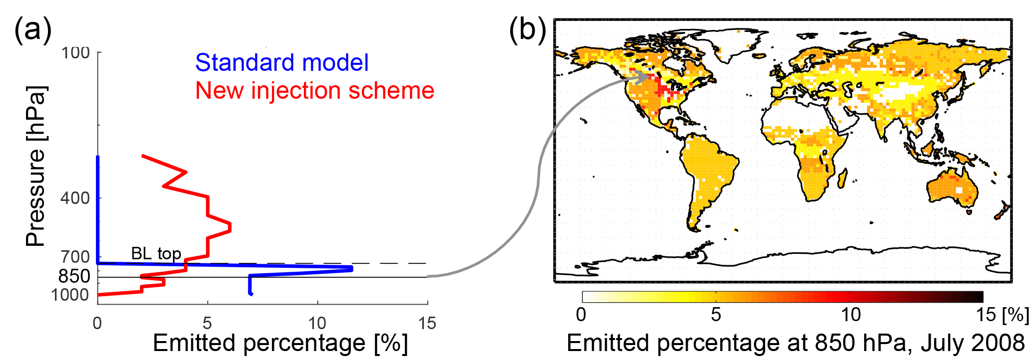
Figure 2(a) Vertical profile of the percent of emissions in each model level for a sample location over boreal Canada (56∘ N, 105∘ W) from the public-release version of GEOS-Chem (blue) and the new observationally based injection scheme (red). The dashed line indicates the averaged boundary layer top of this month. The solid black line is at 850 hPa, corresponding to the layer shown in (b). (b) Percent of total-column biomass burning emissions emitted into the 850 hPa layer in each model grid cell for July 2008.
2.4 GEOS-Chem implementation
We associate the native MISR injection altitude (0–8 km) with the emitted percentages of total biomass burning emissions and map them to the GMAO 47-layer reduced vertical grid and a horizontal grid. The injection percentages of total-column biomass burning emissions for each month for each grid cell are saved in a binary file. Code modifications to read in the data of percentages and distribute the biomass burning emissions to every grid cell are contained within the setemis.F FORTRAN module in GEOS-Chem version 9.01.01. The binary file can be updated based on different analyses (e.g., a more recent year or a different analysis approach), and little effort would be required to update this within the code.
In Fig. 2a, we show an example vertical profile of injection percentages at 56∘ N, 105∘ W from the standard model and the new injection scheme. In contrast to a blanket approach of emitting all biomass burning emissions within the boundary layer, the new injection scheme emits a large percentage of these emissions above the boundary layer at this location. The global map in Fig. 2b shows the injection percentages at 850 hPa in July 2008 for the globe based on the MISR stereo-height data. The amount of the total biomass burning emissions at any given location that are injected into the layer encompassing 850 hPa varies substantially. Figure 2a cannot be interpreted as the total amount of smoke emitted in this layer of the atmosphere; this is a plot of the percent of the total column that the model emits at that level. For example, there are regions during the month of July 2008 with high percentages of emissions injected at a given level but very small total-column emissions overall.
Given the combined limitations in the MISR analysis (Sect. 2.2) and the GFED emissions database at representing small fires, our scheme is unlikely to correctly represent the fraction of total smoke that is emitted above the boundary layer in places where small fires make a significant smoke contribution. Randerson et al. (2012) updated the GFEDv4 inventory to include an estimate of the emissions from fires below the detection limit of the satellite observations used to construct the standard GFED database and most other satellite-based emission inventories. These small fires tend to include agricultural and shrubland fires as well as some grassland fires, peat fires, and ground fires where the overlying tree canopy is dense. The number of small fires is large in some places, their overall contribution to total emissions can be large, and they often produce diffuse, smoky haze rather than discrete plumes that are feasible to map from space. They also tend to inject smoke into the planetary boundary layer rather than above it. These fires are not the focus of the MISR injection height analysis or the MODIS FRP analysis, and although we have attempted to account for this (Sect. 2.2), this is a limitation on our overall approach.
As a final model experiment, we increase the CO emissions by a factor of 1.5 for burning over savannas, a factor of 1.5 for burning associated with deforestation, and a factor of 2 for extratropical forests, following Petrenko et al. (2017). We use horizontal resolution for our global simulations.
2.5 Observational datasets
As a demonstration of the potential impact of the model development and its relevance to a few example regions, we compare GEOS-Chem output with improved injection heights to smoke-impacted trace gas observations from aircraft over boreal North America (July 2008) and from aircraft sites in the Amazon Basin (2010–2011). We also compare the model output to monthly mean surface CO observations in regions impacted by major fires.
2.5.1 North America
Boreal North America is an interesting focal region because emissions from biomass burning lead to enhancements in high-latitude tropospheric ozone during summer (Arnold et al., 2015). The representation of injection height has implications for inverse studies of emissions from fires in this region and the magnitude of the ozone enhancement that results from these emissions (Leung et al., 2007). The second portion of the NASA Arctic Research of the Composition on the Troposphere from Aircraft and Satellites (ARCTAS) mission was conducted over western Canada during June and July 2008. A complete list of species observed by the NASA DC-8 aircraft during ARCTAS can be found in Jacob et al. (2010). In the present study, we use ARCTAS observations of CO and PAN from July 2008 to illustrate the updated performance of the model with the new injection scheme over western North America.
2.5.2 Amazon
We highlight the Amazon Basin as another interesting region as emissions from deforestation fires over Amazonian forests represent a large percent of global emissions from deforestation (van der Werf et al., 2010). Year-to-year variability in this region has been associated with climate extremes (Chen et al., 2013). Thus, it is important to understand the fire injection height over this region in order to fully quantify the impact of these fires on atmospheric composition and to better predict how this impact could evolve in the future. We use the CO observations from four sites across the Amazon Basin in 2010 and 2011: Alta Floresta (ALF; 8.80∘ S, 56.75∘ W), Rio Branco (RBA; 9.38∘ S, 67.62∘ W), Santarém (SAN; 2.86∘ S; 54.95∘ W), and Tabatinga (TAB; 5.96∘ S, 70.06∘ W). Biweekly vertical profiles of CO were measured from just above the forest canopy to 4.4 km above sea level (Gatti et al., 2014). As described in Gatti et al. (2014), samples were collected using a small aircraft. Air samples were collected in flasks that were analyzed using a replica of the NOAA Earth System Research Laboratory (ESRL) trace gas analysis system. The measurements were taken at specific altitude levels on each flight day. Up to six or eight observations are available at each individual altitude level for each month (four sites with two vertical profiles). We also compared model output to aircraft observations from the Balanço Atmosférico Regional de Carbono na Amazônia (BARCA) program, which was deployed in 2008 (Andreae et al., 2012). This dataset contains a strong influence of biomass burning emissions. However, when we sampled the model at the locations of the observations, there were no differences in the simulated CO profiles in the two sets of simulations with the different injection schemes. The CO mixing ratios for the regions were biased low; i.e., model mixing ratios were between 80 and 125 ppb, indicating no smoke influence, whereas the corresponding observations were largely >150 ppb. Andreae et al. (2012) discuss problems with GFEDv3 CO emissions for this region, specifically noting that the emissions in this database could be up to a factor of 7 too low for the BARCA period.

Figure 3(a) Percentage of total-column biomass burning emissions injected above 700 hPa over North America for July 2008, based on MISR observations. The two example locations shown in (b) and (c) are marked as blue stars. (b) Vertical profile of the percent of emissions in each model level over 56∘ N, 105∘ W. (c) Vertical profile of the percent of emissions in each model level over 40∘ N, 82.5∘ W. The dashed line indicates the averaged boundary layer top during this month. BB: biomass burning.
2.5.3 Surface observations
Leung et al. (2007) showed that the choice of injection height for boreal fire emissions impacts the simulation of surface CO mixing ratios in the Northern Hemisphere. They compared GEOS-Chem-simulated anomalies in CO mixing ratios with surface measurements from the NOAA ESRL Global Monitoring Division (GMD) Carbon Cycle Cooperative Air Sampling Network (Novelli et al., 2003). Therefore, we also performed a comparison with monthly mean observations from 21 sites that may have been impacted by fires during 2008. In most locations (16 of 21) where we conducted comparisons, the model with the MISR-based injection height did not produce notably different surface monthly mean CO mixing ratios (i.e., changes are less than 1 ppb). However, there are four stations where the updated model produces substantially lower monthly mean surface CO mixing ratios than the standard model, and this change produces a better simulation of CO at these locations. We present these results in Sect. 3.3.
3.1 North American boreal fires
Figure 3a shows the total percent of biomass burning emissions for each model column emitted above 700 hPa during July 2008 based on MISR observations. We use the 700 hPa level to signify an approximate midday boundary layer top pressure over North America. The percent of emissions injected above 700 hPa in the updated version of the model is quite large over boreal regions, exceeding 60 % for some locations such as the one shown in Fig. 3b. In boreal regions, the majority of biomass burning emissions are produced by a relatively small number of large fires that last days to weeks (Stocks et al., 2002; Brey et al., 2018). Figure 3a shows the strong north–south gradient in the percent of emissions injected above this atmospheric level. In contrast to boreal regions, the new scheme continues to inject nearly all the fire emissions into the boundary layer over the central US during this month. An example profile of the emitted percent by model layer is shown in Fig. 3c. There are typically very few fires during July in this region; those that do occur are typically short-lived and often involve cropland (Brey et al., 2018).
The impact of the new injection scheme on simulated PAN has significant spatial variability over North America during July 2008, and this is driven by the large spatial variability in the fires and the smoke injection level. Figure 4a, b, and c present the differences in simulated PAN mixing ratios between the updated and the standard model at 510 hPa, 850 hPa, and the surface on 1 July 2008, respectively. As expected, the new injection scheme decreases simulated PAN mixing ratios at the surface and within the boundary layer over boreal regions. Simulated PAN mixing ratios increase in the mid and upper troposphere. Figure 6 presents a similar example for 4 July 2008.
Figures 4d and 5d (black lines and open circles) show average vertical profiles of PAN intercepted by the Douglas DC8 jetliner during the ARCTAS flights on these particular days. The NASA DC8 sampled fresh smoke from the Lake McKay fire (56.5∘ N, 106.8∘ W) on 1 July 2008 at several distances downwind (see Alvarado et al., 2010). We sampled both versions of the model along the aircraft pathway at the corresponding observation time, and these average profiles are also plotted in Fig. 4d. In the lower troposphere, the standard model largely overestimates PAN on 1 July 2008 (Fig. 4d). The new injection scheme decreases the simulated PAN in the boundary layer significantly (∼300 pptv) and matches the ARCTAS observations better. The same is not true for the comparison with CO (Fig. 5). The DC8 sampled several plumes above 3 km on 4 July. As described in Alvarado et al. (2010), this was a period with strong updrafts, which led to lofting of biomass burning emissions (Fuelberg et al., 2010). We note that time of day could be very important for these comparisons. The aircraft sampled these plumes in the mid- to late afternoon, so MISR heights are likely underestimates of the actual injection altitudes for the cases shown in Figs. 4–7.
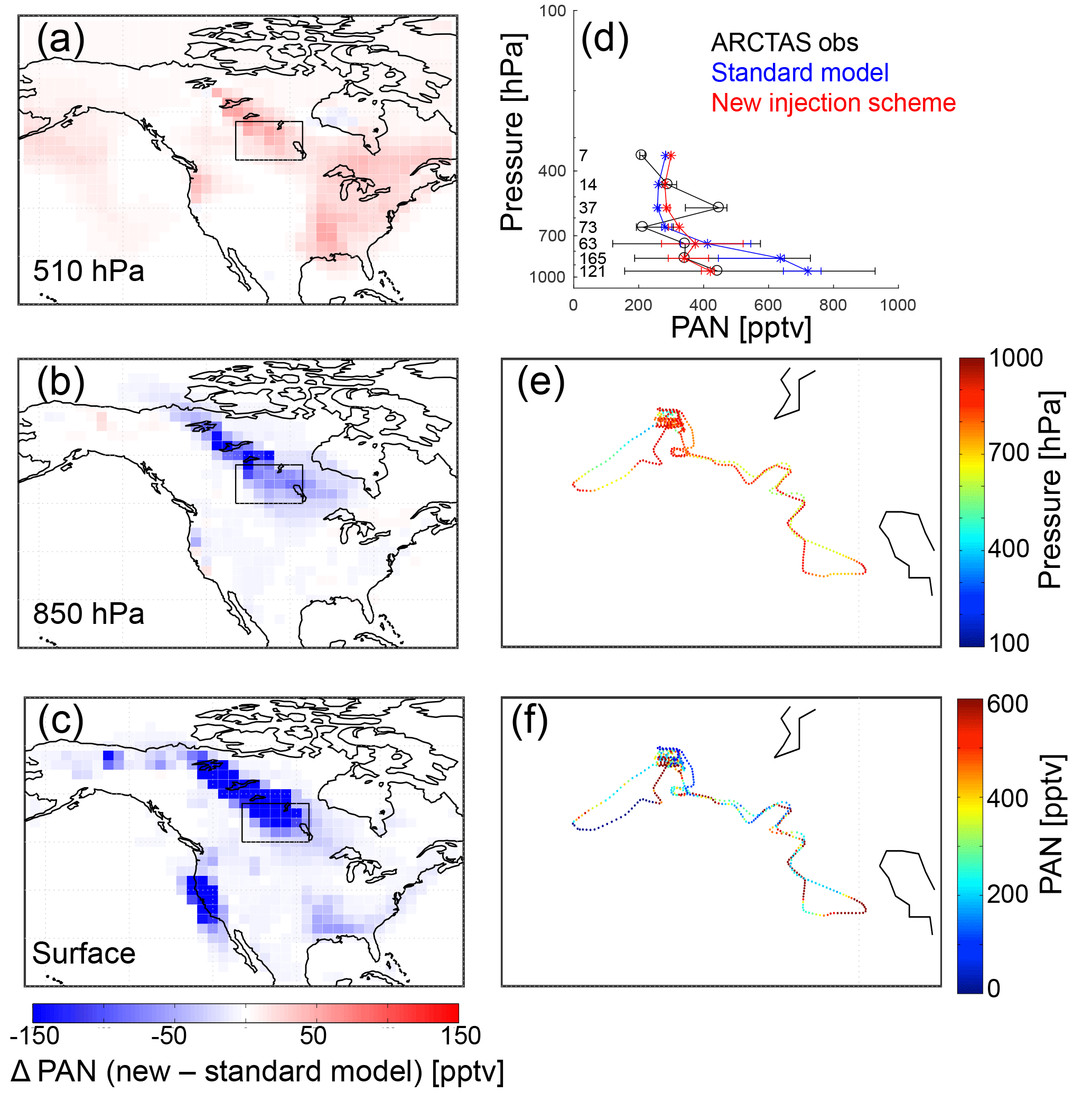
Figure 4(a–c) Differences in simulated PAN mixing ratios between a GEOS-Chem simulation with and without the new observationally based biomass burning injection scheme over North America at three different levels: 510 hPa, 850 hPa, and the surface on 1 July 2008. (d) Median vertical profiles of ARCTAS PAN mixing ratios (black), standard model (blue), and new injection scheme (red) on 1 July 2008. The whiskers represent 25 % and 75 % percentiles of the data in the pressure bins. The numbers on the left are the numbers of observations in different pressure bins. (e) ARCTAS in situ aircraft observations for 1 July 2008 colored by ambient pressure for the inset black box in (a–c). (f) ARCTAS observations for 1 July 2008 colored by PAN mixing ratio.
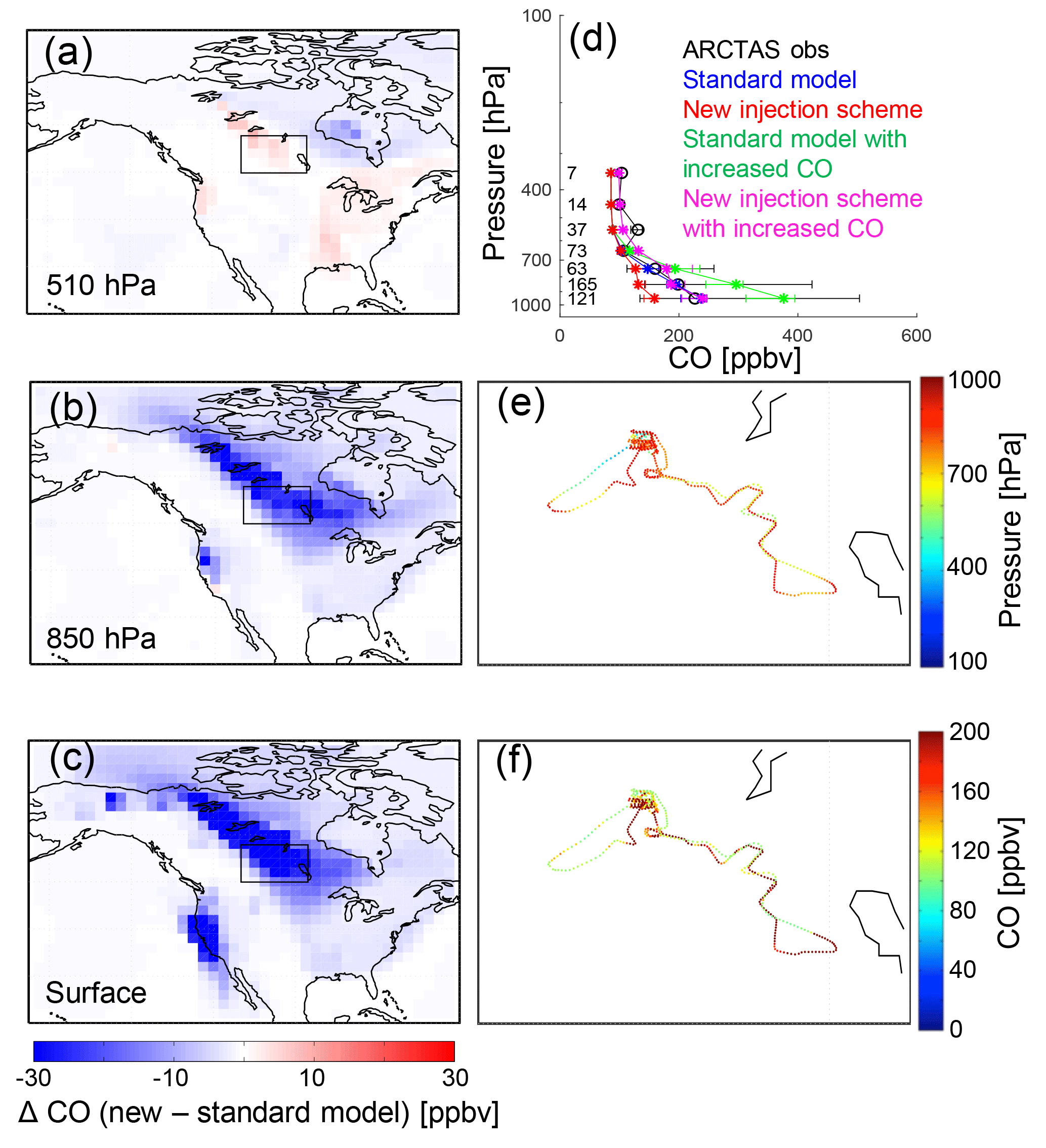
Figure 5Same as in Fig. 4 but for CO. The pink profiles are from a simulation that also increased the emissions of CO from boreal fires as described in Sect. 2.4. The green profiles are from a simulation of the standard model with increased CO emissions as the pink profiles.
On 4 July 2008 (Fig. 6d), the new injection scheme does not change simulated PAN meaningfully near the surface where the aircraft was located. Figure 6e and c show that the aircraft did not fly through the low-altitude regions of the model, which showed important changes from the injection scheme. The near-surface PAN mixing ratios were not impacted south of the Hudson Bay. However, the new injection scheme does increase PAN by ∼130 pptv in the lower to mid free troposphere. This improves the model–measurement comparison substantially between 800 and 500 hPa. The GEOS-Chem simulations presented in Alvarado et al. (2010) substantially underestimated PAN relative to the ARCTAS observations. Here we have included the partitioning of NOx immediately to PAN and HNO3 as originally suggested by Alvarado et al. (2010), and we have updated the injection height. Along with the other updates in Fischer et al. (2014), this appears to greatly improve the ability of the model to simulate the appropriate magnitude of PAN for the cases shown.
Figure 7 presents simulated and observed CO from the 4 July ARCTAS flight. Similar to PAN, for this particular profile the new injection scheme decreases CO in the lower troposphere and increases it in the middle troposphere (Fig. 7d). However, both the standard model and the new injection scheme underestimate CO significantly compared to ARCTAS observations. Both model versions continue to produce a monotonic decrease in CO from the surface to upper levels, and although the new injection scheme increases CO just above 700 hPa, it is not able to simulate the enrichment layer that appears to be present in the observations. The mean CO underestimate shown in Fig. 7d is 15 %–56 %. The model does not appear to have such a low bias for the 1 July case (Fig. 5), but there are very few samples at higher altitudes in this flight. Alvarado et al. (2010) and Fisher et al. (2010) previously compared a GEOS-Chem simulation to ARCTAS observations. The simulation used in those prior studies was based on daily emissions from the Fire Locating and Monitoring of Burning Emissions (FLAMBE) inventory (Reid et al., 2009). Monthly mean GFEDv2 emissions were used for the model spin-up. The FLAMBE inventory overestimated CO emissions from fires in this region (Alvarado et al., 2010). In contrast, we find that CO is underpredicted using GFEDv3 monthly average emissions.


Figure 7Same as in Fig. 5 but for 4 July 2008. The pink profiles are from a simulation that also increased the emissions of CO from boreal fires as described in Sect. 2.4. The green profiles are from a simulation of the standard model, with increased CO emissions as the pink profiles.
We do not aim to optimize the ability of the model to simulate these specific plumes but rather to show the magnitude of the changes with respect to this well-studied set of plumes. Chen et al. (2009) found that switching from monthly to 8-day time intervals for GFEDv2 in GEOS-Chem had the largest effect on simulating measured day-to-day variability in CO for boreal fires during the 2004 fire season. So it is possible that this approach (or alternatively using daily or 3-hourly fire fractions) would also improve the ability of the model to capture these specific plumes. However, both the daily or 3-hourly emissions inventories in our case are still likely to be an underestimate of the true emissions. Thus, we did not pursue these options. However, to simply show the impact of changing the emission factors, we include an additional simulation (pink line in Fig. 7d) with both the updated injection scheme and increased emissions of CO (factor of 2 for extratropical fires and 1.5 for savannas) following Petrenko et al. (2017), which has successfully reproduced the satellite observations of aerosol optical depth (AOD) with a series of adjustments to biomass burning emissions. We also include results from a standard model simulation with increased CO emissions (green line in Fig. 7d). The green line indicates that this model configuration substantially increases the CO mixing ratios within the boundary layer as expected. Comparing this simulation (green line in Fig. 7d) to the simulation incorporating both the new injection scheme and increased CO emissions (pink line in Fig. 7d) shows the impact of both changes. By comparison, CO is higher at levels above the boundary layer and slightly lower in the boundary layer.
3.2 Amazon Basin comparison
As discussed in Sect. 2.5.2, we compare the simulated CO profiles to observed CO profiles at four Amazon Basin sites in each month during 2010 and 2011. We note that we evaluated GEOS-Chem over the Amazon with observations collected in different years than the MISR plume-height data used to develop the parameterization. We made this choice because 2010–2011 CO profiles are available for use in the model–measurement comparison, and the MISR smoke-plume-height climatology from 2005 to 2012 shows little interannual variability over this region (Gonzalez-Alonso et al., 2018). Where the data and the model are clearly smoke-impacted, a simulation that includes both the new injection scheme and increased CO emissions does improve the simulated CO profiles over this region. Figure 8 shows the total emitted percent of biomass burning emission injected above 700 hPa over the Amazon from March to November based on the MISR data. We note that 700 hPa is above the boundary layer in this location. The boundary layer in this region typically extends to 1200–1500 m above ground level in the morning to early afternoon, which corresponds to 880–840 hPa. From March to August, the total emitted percent in each grid cell above 700 hPa over the Amazon area is generally <15 %. Thus, the new injection scheme does not produce a large difference in simulated CO profiles compared to the baseline simulation. However, the total emitted percent above 700 hPa in each grid cell is generally >25 % from September to November. Figure 9b shows the vertical profiles of the emitted percent of biomass burning smoke from the standard model and the new injection scheme at the RBA site for one case in October. Although peak emitted percentages in both simulations are near the top of the boundary layer, the new injection scheme has the emissions pushed higher in the atmosphere. Figure 9c shows a comparison of the simulations with the corresponding biweekly observations at RBA in October of 2010 and 2011. Above the lowermost kilometers, the simulated CO from the standard model generally underpredicts the observed CO mixing ratios. The new injection scheme decreases CO mixing ratios in the boundary layer (by up to 45 ppb) and increases CO mixing ratios in the troposphere (by up to 12 ppb). CO mixing ratios are 20–75 ppb lower than the RBA observations. With the increased CO emissions (pink), simulated CO mixing ratios near the surface provide a better match to the observations than the other two model versions. Away from the surface the simulation that includes both increased CO and the new injection scheme also performs better that the other two model versions, but the model still underpredicts CO mixing ratios in this region of the atmosphere by ∼50 ppb.
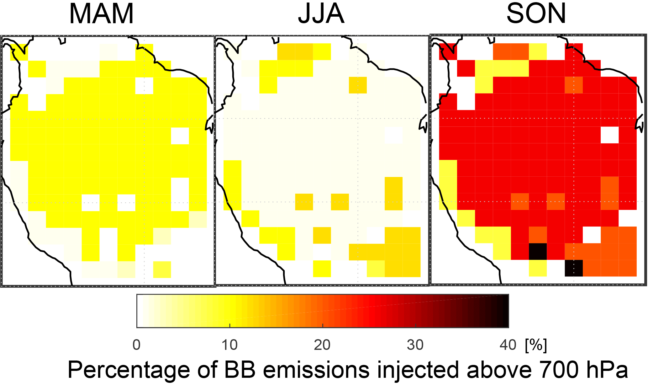
Figure 8Percentage of total-column biomass burning emissions injected above 700 hPa over the Amazon from March to November of 2010 and 2011, based on MISR plume-height analysis.
We also compared the model output to the CO mixing ratio profiles over the other three sites (TAB, ALF, and SAN), and the impact of new injection scheme on CO mixing ratios at all levels over all three locations is small. Consistent with Andreae et al. (2012), we also found that the simulated CO mixing ratios are generally underpredicted in all months, especially during the biomass burning seasons. For example, the simulated CO mixing ratios are almost 3 times lower than observations in September at the SAN site. Gatti et al. (2014) found an emission ratio of 72.8 ppb CO ∕ CO2 ppm. For comparison the emission ratios used in GFEDv3 as implemented in GEOS-Chem are 97.5 and 59.5 ppb CO ∕ CO2 ppm for deforestation and savannas, respectively. It is possible that either the emission factors themselves may be too low in GFEDv3 or there are fires missing from the inventory, so redistributing them in the atmosphere is not sufficient to better simulate their impact on atmospheric composition.
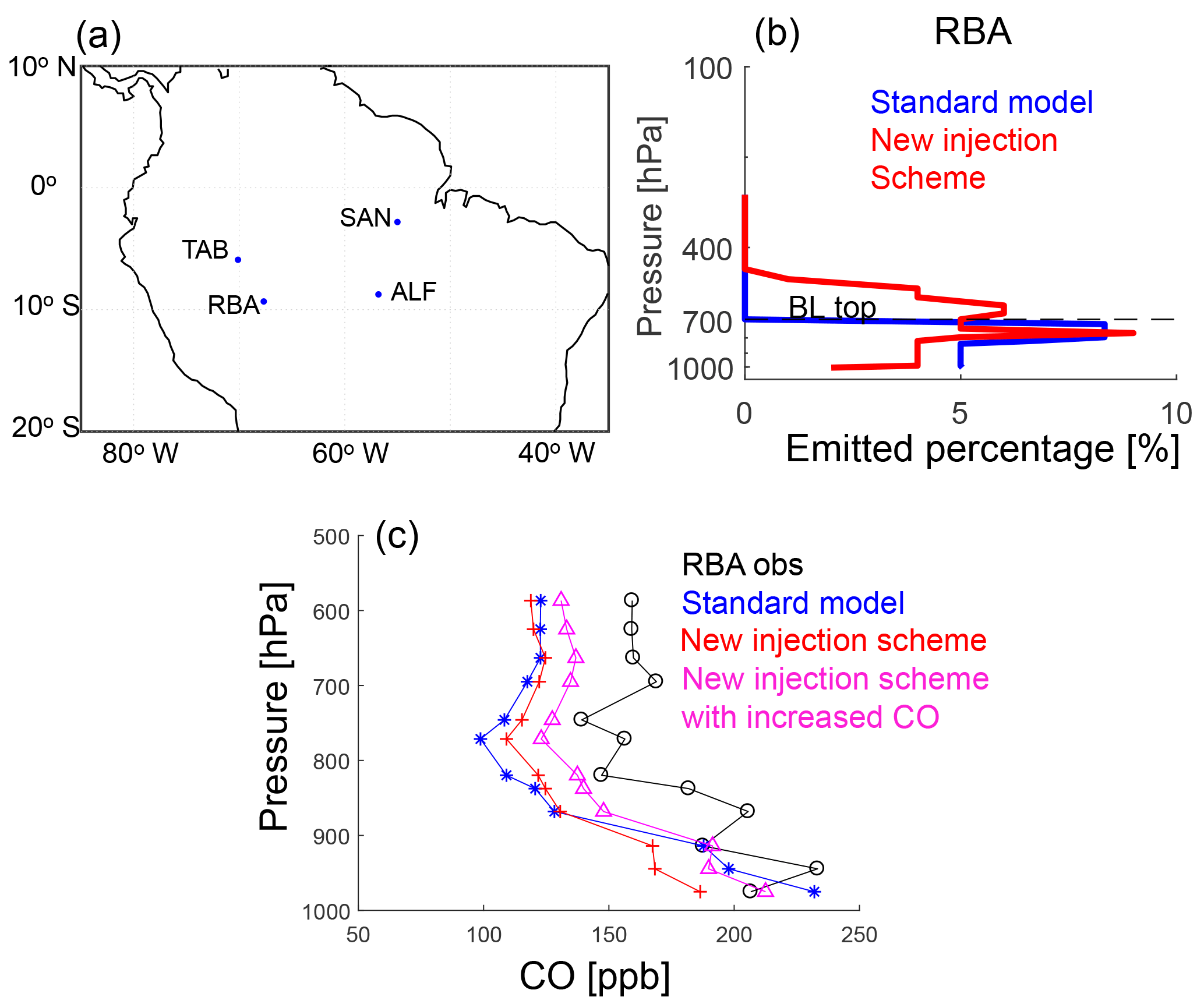
Figure 9(a) Map of four measurement sites in the Amazon Basin. (b) Vertical profile of the percent of emissions in each model level at site RBA from the public-release version of GEOS-Chem (blue) and the new observationally based injection scheme (red). The dashed line indicates the averaged boundary layer top during this month. (c) Median vertical profiles of CO mixing ratios observed at RBA (black), simulated with the standard model (blue), simulated with the new injection scheme (red), and simulated with the new injection scheme and with increased CO (Petrenko et al., 2017) in October of 2010 and 2011.
3.3 Averaged impacts on CO
As the case studies of individual plumes presented in Sect. 3.1 and 3.2 show, injecting the emissions of boreal fires higher in the atmosphere often increases the CO mixing ratio in the mid troposphere above and directly downwind of the fire. For the 4 July smoke plume from ARCTAS (Fig. 7), the new model substantially reduces CO mixing ratios near the surface and at 850 hPa. There is an increase in CO at 510 hPa directly above and directly downwind of the fire as compared to the standard model (Fig. 7a). However, Fig. 7a also shows a decrease in CO at 510 hPa over much, but not all, of the domain. When viewed hemispherically, the net effect of lofting emissions out of the boundary layer is to produce lower average CO mixing ratios in the mid upper troposphere because the average lifetime of CO against oxidation by OH is slightly shorter. Annual and globally averaged concentrations of OH increase slightly with altitude from 1000 to 700 hPa (Spivakovsky et al., 2000). Thus, when a fraction of the CO emissions are immediately moved out of the boundary layer, this fraction reacts more quickly with OH than in the standard simulation. The same issue applies throughout the atmosphere and can be visualized for the Amazon region in Fig. 9c. The CO mixing ratio decreases with altitude above 650 hPa at a faster rate in the simulation with the new injection scheme than in the standard model. This effect is not local to a given fire but reflects the cumulative impact of changing the emission altitude for a substantial quantity of CO emissions. In our model, the resulting changes to monthly mean CO are not large, but there is quite a bit of variability by season and location. Typical monthly mean decreases in CO mixing ratios away from freshly injected biomass burning plumes are <5 % in the mid to upper troposphere. The changes in CO between model versions reflect changed injection heights throughout the Northern Hemisphere, not just the fire producing the particular smoke sampled by the aircraft that day. The response of CO is very different than that of PAN. The main loss of PAN is via thermal decomposition, so injecting PAN (or its precursors) higher in the atmosphere will increase PAN in the mid to upper troposphere. Though we highlight CO and PAN here as examples, injection height will impact the chemical evolution of nearly all species emitted from fires.
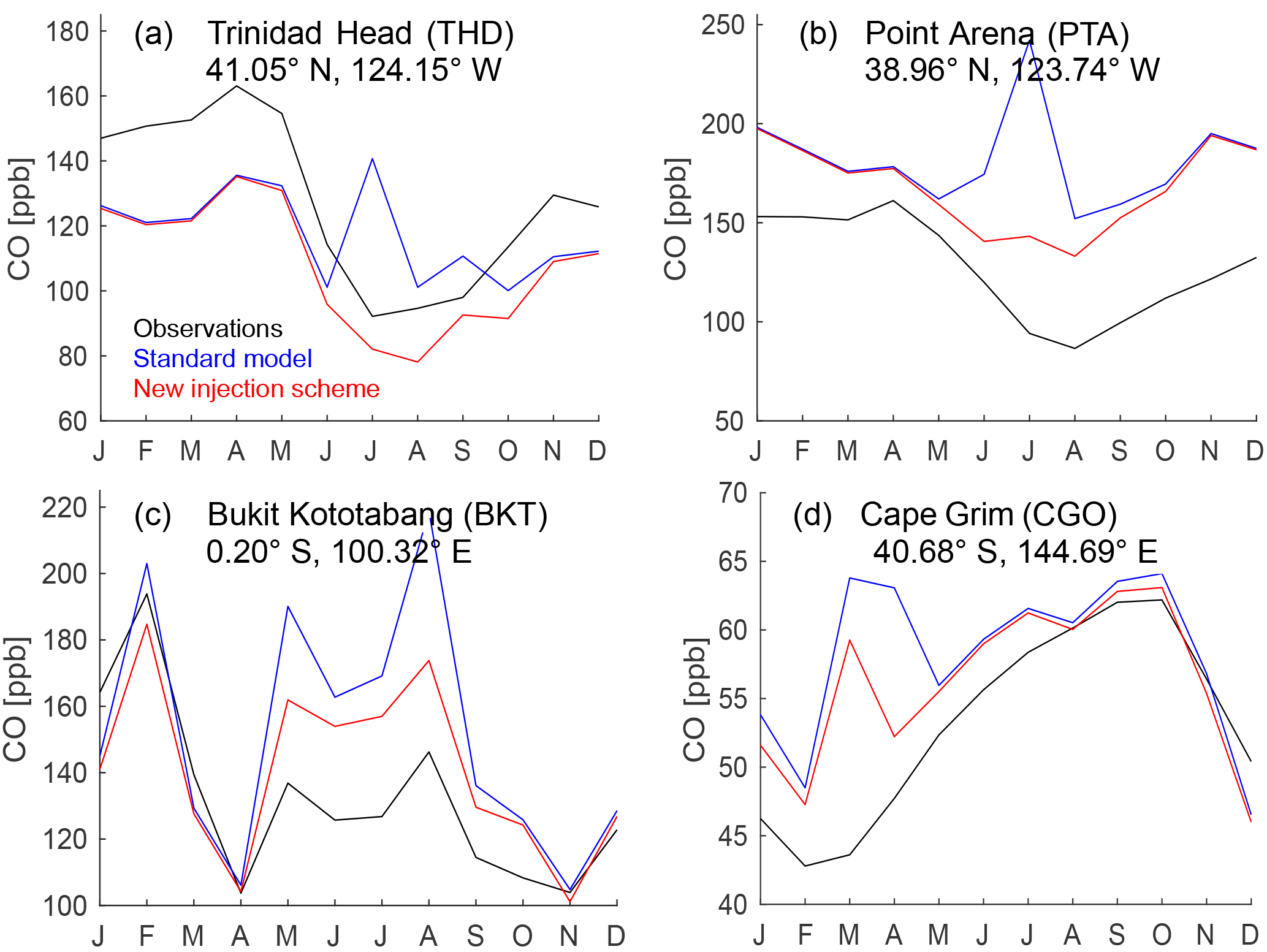
Figure 10Observed and simulated monthly mean CO mixing ratios at select NOAA ESRL Carbon Cycle Cooperative Global Air Sampling Network sites.
Figure 10 shows a comparison of our different model versions to monthly mean surface CO mixing ratios from four sites where there are substantial changes in 2008 monthly mean simulated CO with the new injection scheme. The decreases in simulated surface CO can be substantial when the emissions are moved up higher in the atmosphere based on the MISR analysis. Figure 10a and b indicate that the standard model overpredicts July 2008 surface CO mixing ratios at two California monitoring sites: Trinidad Head and Point Arena. There were hundreds of wildfires in northern California in June and July 2008 (Gyawali et al., 2009; Brey et al., 2018). The model with the improved injection height parameterization removes a large CO peak in July that is clearly not present in the surface observations. The lower panels of Fig. 10 indicate that the model overpredicts surface CO abundances during much of the year at these two sites in the Southern Hemisphere: Bukit Kototabang (BKT), Indonesia, and Cape Grim (CGO), Tasmania. However, the updated version of the model does reduce the model–measurement discrepancy at BKT between March and September 2008 by ∼50 %.
This paper introduces the development and implementation of a new global biomass burning emissions injection scheme in the GEOS-Chem model. The injection scheme is based on a MISR plume-injection-height climatology for 2008. This climatology was derived from space-based, multi-angle imagery. Additional (i.e., based on other datasets) or updated (i.e., other years) gridded climatologies of injection height could be implemented with relatively little effort given the code infrastructure that is now in place. We have completed multiyear simulations with the new injection scheme and compared the model output to three smoke-impacted observational datasets.
Based on MISR snapshots, the percentage of total-column biomass burning emissions that are typically injected above the boundary layer is relatively high for North American boreal regions. We find that the updated model is better able to simulate observed daytime observed vertical profiles of PAN and CO over boreal regions during the 2008 summer fire season, and including a better representation of injection height is likely very important for predicting the transport and chemical evolution of smoke plumes originating in this region. However, the version of GEOS-Chem used here has a persistent low bias in CO throughout the atmospheric column. Though our injection height climatology is based on observations from 2008, we also used this to simulate October 2010 and 2011 for the Amazon region. We made this choice because this season provided access to CO profiles that could be used for model–measurement comparison, and for this region, smoke injection heights do not appear to vary much interannually.
In testing our model updates, we consistently found that it was important to do model–observation comparisons on specific biomass burning plumes with a well-sampled vertical structure. When the model is sampled to match observations with less vertical information (e.g., Measurements of Pollution in the Troposphere (MOPITT) CO or Tropospheric Emission Spectrometer (TES) PAN retrievals), the differences between the simulations appeared very small. However, when the model is compared to specific plumes, an improved injection height does produce notable differences in the simulations that can have air quality and possibly climate implications (see also Vernon et al., 2018). Thus, moving forward, we recommend that simulations with improved vertical injection height schemes for biomass burning plumes be compared to specific plumes rather than larger-scale observations.
It is important to note that the MISR plume heights that form the basis for our injection scheme are only snapshots. MISR is in a sun-synchronous orbit, and it crosses the Equator at 10:30 local time. Actual wildfire smoke injection heights vary diurnally and less predictably hour to hour or day to day as burning progresses. Our scheme provides one consistent, statistically based injection height for each month; however, the ARCTAS aircraft observations also represent daytime measurements. A future development may be to attempt to anchor the model plume height at the MISR overpass time rather than assuming a constant plume height. A better comparison would include plumes observed throughout the diurnal cycle.
Though these model developments offer clear improvements under some situations, limitations in this approach should be noted. Most importantly, the MISR climatology that underpins this model development is based on snapshots of injection height. Thus, it may not apply to all fires at a given location at all times of day. The MISR plume-height climatology also may not represent the injection height of small fires as well as it does that of larger ones. We expect that this approach will be most appropriate in regions where the total smoke emissions are dominated by fires large enough to be observed by the satellite instrument. However, most small fires inject only into the boundary layer, so if the amount of small-fire smoke is available, its vertical distribution can be assumed with some confidence.
The GEOS-Chem code used to generate this paper has already been passed to the GEOS-Chem model support team, and we currently plan to include it as an option in the next public version of the model. The anticipated release date will be prior to publication. The code and data used for this study are published as a Supplement and can be directly applied to the work based on GEOS-Chem v9-01-01. The aircraft and surface data used in this paper are already publically available.
The supplement related to this article is available online at: https://doi.org/10.5194/gmd-11-4103-2018-supplement.
LZ led the majority of the analysis associated with this paper. MVM led the analysis of the MISR data and developed the monthly average gridded climatology of plume heights for 2008. AH provided the smoke designation associated with the ARCTAS aircraft data. LVG led the aircraft measurements over the Amazon Basin. RK helped develop the MISR plume-height algorithm and led or mentored much of its application to wildfire smoke and volcanic plumes. EVF led the conception of the work and the writing of this paper.
The authors declare that they have no conflict of interest.
This work was supported by NASA award numbers NNX14AF14G
and NNX14AN47G. PAN data from ARCTAS were provided by Greg Huey supported by
NASA award number NNX08AR67G. Amazon vertical profile data were provided by
Luciana V. Gatti supported by NERC (NE/F005806/1) and FAPESP (08/58120-3). We
thank Glenn Diskin for the use of the ARCTAS CO data. We thank
Paul C. Novelli for the use of the CO data from NOAA ESRL Carbon Cycle
Cooperative Global Air Sampling Network. Maria Val Martin was partially
supported by the Leverhulme Trust through a Leverhulme Research Centre Award
(RC-2015-029). Ralph Kahn is supported in part by NASA's Climate and
Radiation Research and Analysis Program under Hal Maring and NASA's Atmospheric Composition Program under
Richard Eckman.
Edited by: Jason Williams
Reviewed by: two
anonymous referees
Akagi, S. K., Yokelson, R. J., Wiedinmyer, C., Alvarado, M. J., Reid, J. S., Karl, T., Crounse, J. D., and Wennberg, P. O.: Emission factors for open and domestic biomass burning for use in atmospheric models, Atmos. Chem. Phys., 11, 4039–4072, https://doi.org/10.5194/acp-11-4039-2011, 2011.
Alvarado, M. J., Logan, J. A., Mao, J., Apel, E., Riemer, D., Blake, D., Cohen, R. C., Min, K.-E., Perring, A. E., Browne, E. C., Wooldridge, P. J., Diskin, G. S., Sachse, G. W., Fuelberg, H., Sessions, W. R., Harrigan, D. L., Huey, G., Liao, J., Case-Hanks, A., Jimenez, J. L., Cubison, M. J., Vay, S. A., Weinheimer, A. J., Knapp, D. J., Montzka, D. D., Flocke, F. M., Pollack, I. B., Wennberg, P. O., Kurten, A., Crounse, J., Clair, J. M. St., Wisthaler, A., Mikoviny, T., Yantosca, R. M., Carouge, C. C., and Le Sager, P.: Nitrogen oxides and PAN in plumes from boreal fires during ARCTAS-B and their impact on ozone: an integrated analysis of aircraft and satellite observations, Atmos. Chem. Phys., 10, 9739–9760, https://doi.org/10.5194/acp-10-9739-2010, 2010.
Andreae, M. O., Artaxo, P., Beck, V., Bela, M., Freitas, S., Gerbig, C., Longo, K., Munger, J. W., Wiedemann, K. T., and Wofsy, S. C.: Carbon monoxide and related trace gases and aerosols over the Amazon Basin during the wet and dry seasons, Atmos. Chem. Phys., 12, 6041–6065, https://doi.org/10.5194/acp-12-6041-2012, 2012.
Arnold, S. R., Emmons, L. K., Monks, S. A., Law, K. S., Ridley, D. A., Turquety, S., Tilmes, S., Thomas, J. L., Bouarar, I., Flemming, J., Huijnen, V., Mao, J., Duncan, B. N., Steenrod, S., Yoshida, Y., Langner, J., and Long, Y.: Biomass burning influence on high-latitude tropospheric ozone and reactive nitrogen in summer 2008: a multi-model analysis based on POLMIP simulations, Atmos. Chem. Phys., 15, 6047–6068, https://doi.org/10.5194/acp-15-6047-2015, 2015.
Boy, J., Rollenbeck, R., Valarezo, C., and Wilcke, W.: Amazonian biomass burning-derived acid and nutrient deposition in the north Andean montane forest of Ecuador, Global Biogeochem. Cy., 22, GB4011, https://doi.org/10.1029/2007GB003158, 2008.
Bey, I., Jacob, D. J., Yantosca, R. M., Logan, J. A., Field, B. D., Fiore, A. M., Li, Q., Liu, H. Y., Mickley, L. J., and Schultz, M. G.: Global modeling of tropospheric chemistry with assimilated meteorology: Model description and evaluation, J. Geophys. Res., 106, 23073–23095, https://doi.org/10.1029/2001JD000807, 2001.
Brey, S. J., Ruminski, M., Atwood, S. A., and Fischer, E. V.: Connecting smoke plumes to sources using Hazard Mapping System (HMS) smoke and fire location data over North America, Atmos. Chem. Phys., 18, 1745–1761, https://doi.org/10.5194/acp-18-1745-2018, 2018.
Brey, S. J., Ruminski, M., Atwood, S. A., and Fischer, E. V.: Connecting smoke plumes to sources using Hazard Mapping System (HMS) smoke and fire location data over North America, Atmos. Chem. Phys., 18, 1745–1761, https://doi.org/10.5194/acp-18-1745-2018, 2018.
Chen, Y., Li, Q., Randerson, J. T., Lyons, E. A., Kahn, R. A., Nelson, D. L., and Diner, D. J.: The sensitivity of CO and aerosol transport to the temporal and vertical distribution of North American boreal fire emissions, Atmos. Chem. Phys., 9, 6559–6580, https://doi.org/10.5194/acp-9-6559-2009, 2009.
Chen, Y., Morton, D. C., Jin, Y., Collatz, G. J., Kasibhatla, P. S., van der Werf, G. R., DeFries, R. S., and Randerson, J. T.: Long-term trends and interannual variability of forest, savanna and agricultural fires in South America, Carbon Manag., 4, 617–638, https://doi.org/10.4155/cmt.13.61, 2013.
Colarco, P. R., Schoeberl, M. R., Doddridge, B. G., Marufu, L. T., Torres, O., and Welton, E. J.: Transport of smoke from Canadian forest fires to the surface near Washington, DC: Injection height, entrainment, and optical properties, J. Geophys. Res.-Atmos., 109, D06203, https://doi.org/10.1029/2003JD004248, 2004.
Damoah, R., Spichtinger, N., Forster, C., James, P., Mattis, I., Wandinger, U., Beirle, S., Wagner, T., and Stohl, A.: Around the world in 17 days – hemispheric-scale transport of forest fire smoke from Russia in May 2003, Atmos. Chem. Phys., 4, 1311–1321, https://doi.org/10.5194/acp-4-1311-2004, 2004.
Diner, D. J., Beckert, J. C., Reilly, T. H., Bruegge, C. J., Conel, J. E., Kahn, R. A., Martonchik, J. V., Ackerman, T. P., Davies, R., Gerstl, A. W., Gordon, H. R., Muller, J.-P., Myneni, R. B., Sellers, P. J., Pinty, B., and Verstraete, M. M.: Multi-angle imaging spectroradiometer (MISR) instrument description and experiment overview, IEEE T. Geosci. Remote, 36, 1072–1087, https://doi.org/10.1109/36.700992, 1998.
Emmons, L. K., Arnold, S. R., Monks, S. A., Huijnen, V., Tilmes, S., Law, K. S., Thomas, J. L., Raut, J.-C., Bouarar, I., Turquety, S., Long, Y., Duncan, B., Steenrod, S., Strode, S., Flemming, J., Mao, J., Langner, J., Thompson, A. M., Tarasick, D., Apel, E. C., Blake, D. R., Cohen, R. C., Dibb, J., Diskin, G. S., Fried, A., Hall, S. R., Huey, L. G., Weinheimer, A. J., Wisthaler, A., Mikoviny, T., Nowak, J., Peischl, J., Roberts, J. M., Ryerson, T., Warneke, C., and Helmig, D.: The POLARCAT Model Intercomparison Project (POLMIP): overview and evaluation with observations, Atmos. Chem. Phys., 15, 6721–6744, https://doi.org/10.5194/acp-15-6721-2015, 2015.
Fischer, E. V., Jacob, D. J., Yantosca, R. M., Sulprizio, M. P., Millet, D. B., Mao, J., Paulot, F., Singh, H. B., Roiger, A., Ries, L., Talbot, R. W., Dzepina, K., and Pandey Deolal, S.: Atmospheric peroxyacetyl nitrate (PAN): a global budget and source attribution, Atmos. Chem. Phys., 14, 2679–2698, https://doi.org/10.5194/acp-14-2679-2014, 2014.
Fisher, J. A., Jacob, D. J., Purdy, M. T., Kopacz, M., Le Sager, P., Carouge, C., Holmes, C. D., Yantosca, R. M., Batchelor, R. L., Strong, K., Diskin, G. S., Fuelberg, H. E., Holloway, J. S., Hyer, E. J., McMillan, W. W., Warner, J., Streets, D. G., Zhang, Q., Wang, Y., and Wu, S.: Source attribution and interannual variability of Arctic pollution in spring constrained by aircraft (ARCTAS, ARCPAC) and satellite (AIRS) observations of carbon monoxide, Atmos. Chem. Phys., 10, 977–996, https://doi.org/10.5194/acp-10-977-2010, 2010.
Forster, C., Wandinger, U., Wotawa, G., James, P., Mattis, I., Althausen, D., Simmonds, P., O'Doherty, S., Jennings, S. G., Kleefeld, C., Schneider, J., Trickl, T., Kreipl, S., Jäger, H., and Stohl, A.: Transport of boreal forest fire emissions from Canada to Europe, J. Geophys. Res.-Atmos., 106, 22887–22906, https://doi.org/10.1029/2001JD900115, 2001.
Freitas, S. R., Longo, K. M., and Andreae, M. O.: Impact of including the plume rise of vegetation fires in numerical simulations of associated atmospheric pollutants, Geophys. Res. Lett., 33, L17808, https://doi.org/10.1029/2006GL026608, 2006.
Friedl, M. A., Sulla-Menashe, D., Tan, B., Schneider, A., Ramankutty, N., Sibley, A., and Huang, A. M.: MODIS Collection 5 global land cover: Algorithm refinements and characterization of new datasets, Remote Sens. Environ., 168–182, https://doi.org/10.1016/j.rse.2009.08.016, 2010.
Fuelberg, H. E., Harrigan, D. L., and Sessions, W.: A meteorological overview of the ARCTAS 2008 mission, Atmos. Chem. Phys., 10, 817–842, https://doi.org/10.5194/acp-10-817-2010, 2010.
Gatti, L. V., Gloor, M., Miller, J. B., Doughty, C. E., Malhi, Y., Domingues, L. G., Basso, L. S., Martinewski, A., Correia, C. S. C., Borges, V. F., Freitas, S., Braz, R., Anderson, L. O., Rocha, H., Grace, J., Phillips, O. L., and Lloyd, J.: Drought sensitivity of Amazonian carbon balance revealed by atmospheric measurements, Nature, 506, 76–80, https://doi.org/10.1038/nature12957, 2014.
Gonzalez-Alonso, L., Val Martin, M., and Kahn, R. A.: Biomass burning smoke heights over the Amazon observed from space, Atmos. Chem. Phys. Discuss., https://doi.org/10.5194/acp-2018-931, in review, 2018.
Gonzi, S., Palmer, P. I., Paugam, R., Wooster, M., and Deeter, M. N.: Quantifying pyroconvective injection heights using observations of fire energy: sensitivity of spaceborne observations of carbon monoxide, Atmos. Chem. Phys., 15, 4339–4355, https://doi.org/10.5194/acp-15-4339-2015, 2015.
Gyawali, M., Arnott, W. P., Lewis, K., and Moosmüller, H.: In situ aerosol optics in Reno, NV, USA during and after the summer 2008 California wildfires and the influence of absorbing and non-absorbing organic coatings on spectral light absorption, Atmos. Chem. Phys., 9, 8007–8015, https://doi.org/10.5194/acp-9-8007-2009, 2009.
Jacob, D. J., Crawford, J. H., Maring, H., Clarke, A. D., Dibb, J. E., Emmons, L. K., Ferrare, R. A., Hostetler, C. A., Russell, P. B., Singh, H. B., Thompson, A. M., Shaw, G. E., McCauley, E., Pederson, J. R., and Fisher, J. A.: The Arctic Research of the Composition of the Troposphere from Aircraft and Satellites (ARCTAS) mission: design, execution, and first results, Atmos. Chem. Phys., 10, 5191–5212, https://doi.org/10.5194/acp-10-5191-2010, 2010.
Jian, Y. and Fu, T.-M.: Injection heights of springtime biomass-burning plumes over peninsular Southeast Asia and their impacts on long-range pollutant transport, Atmos. Chem. Phys., 14, 3977–3989, https://doi.org/10.5194/acp-14-3977-2014, 2014.
Kahn, R. A., Chen, Y., Nelson, D. L., Leung, F.-Y., Li, Q., Diner, D. J., and Logan, J. A.: Wildfire smoke injection heights: Two perspectives from space, Geophys. Res. Lett., 35, L04809, https://doi.org/10.1029/2007GL032165, 2008.
Kaiser, J. W., Heil, A., Andreae, M. O., Benedetti, A., Chubarova, N., Jones, L., Morcrette, J.-J., Razinger, M., Schultz, M. G., Suttie, M., and van der Werf, G. R.: Biomass burning emissions estimated with a global fire assimilation system based on observed fire radiative power, Biogeosciences, 9, 527–554, https://doi.org/10.5194/bg-9-527-2012, 2012.
Leung, F. T., Logan, J. A., Park, R., Hyer, E., Kasischke, E., Streets, D., and Yurganov, L.: Impacts of enhanced biomass burning in the boreal forests in 1998 on tropospheric chemistry and the sensitivity of model results to the injection height of emissions, J. Geophys. Res.-Atmos., 112, D10313, https://doi.org/10.1029/2006JD008132, 2007.
Lewis, A. C., Evans, M. J., Hopkins, J. R., Punjabi, S., Read, K. A., Purvis, R. M., Andrews, S. J., Moller, S. J., Carpenter, L. J., Lee, J. D., Rickard, A. R., Palmer, P. I., and Parrington, M.: The influence of biomass burning on the global distribution of selected non-methane organic compounds, Atmos. Chem. Phys., 13, 851–867, https://doi.org/10.5194/acp-13-851-2013, 2013.
Ichoku, C. and Kaufman, Y. J.: A method to derive smoke emission rates from MODIS fire radiative energy measurements, IEEE T. Geosci. Remote, 43, 2636–2649, 2005.
Mims, S. R., Kahn, R. A., Moroney, C. M., Gaitley, B. J., Nelson, D. L., and Garay, M. J.: MISR Stero-heights of grassland fire smoke plumes in Australia, IEEE T. Geosci. Remote, 48, 25–35, https://doi.org/10.1109/TGRS.2009.2027114, 2010.
Moxim, W. J., Levy, H., and Kasibhatla, P. S.: Simulated global tropospheric PAN: Its transport and impact on NOx, J. Geophys. Res.-Atmos., 101, 12621–12638, https://doi.org/10.1029/96JD00338, 1996.
Nelson, L. D., Garay, J. M., Kahn, A. R., and Dunst, A. B.: Stereoscopic Height and Wind Retrievals for Aerosol Plumes with the MISR INteractive eXplorer (MINX), Remote Sens., 5, 4593–4628, https://doi.org/10.3390/rs5094593, 2013.
Novelli, P. C., Masarie, K. A., Lang, P. M., Hall, B. D., Myers, R. C., and Elkins, J. W.: Reanalysis of tropospheric CO trends: Effects of the 1997–1998 wildfires, J. Geophys. Res.-Atmos., 108, 4464, https://doi.org/10.1029/2002JD003031, 2003.
Paugam, R., Wooster, M., Freitas, S., and Val Martin, M.: A review of approaches to estimate wildfire plume injection height within large-scale atmospheric chemical transport models, Atmos. Chem. Phys., 16, 907–925, https://doi.org/10.5194/acp-16-907-2016, 2016.
Petrenko, M., Kahn, R., Chin, M., and Limbacher, J.: Refined Use of Satellite Aerosol Optical Depth Snapshots to Constrain Biomass Burning Emissions in the GOCART Model, J. Geophys. Res.-Atmos., 122, 10983–11004, https://doi.org/10.1002/2017JD026693, 2017.
Randerson, J. T., Chen, Y., Werf, G. R., Rogers, B. M., and Morton, D. C.: Global burned area and biomass burning emissions from small fires, J. Geophys. Res., 117, G04012, https://doi.org/10.1029/2012JG002128, 2012.
Reid, J. S., Hyer, E. J., Prins, E. M., Westphal, D. L., Wang, J., Chritopher, S. A., Curtis, C. A., Schmidt, C. C., Eleuterio, D. P., Richardson, K. A., and Hoffman, J. P.: Global Monitoring and Forecasting of Biomass-Burning Smoke: Description of and Lessons From the Fire Locating and Modeling of Burning Emissions (FLAMBE) Program, IEEE J. Sel. Top. Appl., 2, 144–162, 2009.
Singh, H. B. and Hanst, P. L.: Peroxyacetyl nitrate (PAN) in the unpolluted atmosphere: An important reservoir for nitrogen oxides, Geophys. Res. Lett., 8, 941–944, https://doi.org/10.1029/GL008i008p00941, 1981.
Spivakovsky, C. M., Logan, J. A., Montzka, S. A., Balkanski, Y. J., Foreman-Fowler, M., Jones, D. B. A., Horowitz, L. W., Fusco, A. C., Brenninkmeijer, C. A. M., Prather, M. J., Wofsy, S. C., and McElroy, M. B.: Three-dimensional climatological distribution of tropospheric OH: Update and evaluation, J. Geophys. Res.-Atmos., 105, 8931–8980, https://doi.org/10.1029/1999JD901006, 2000.
Stein, A. F., Rolph, G. D., Draxler, R. R., Stunder, B., and Ruminski, M.: Verification of the NOAA Smoke Forecasting System: Model Sensitivity to the Injection Height, Weather Forecast., 24, 379–394, https://doi.org/10.1175/2008WAF2222166.1, 2009.
Stocks, B. J., Mason, J. A., Todd, J. B., Bosch, E. M., Wotton, B. M., Amiro, B. D., Flannigan, M. D., Hirsch, K. G., Logan, K. A., Martell, D. L., and Skinner, W. R.: Large forest fires in Canada, 1959–1997, J. Geophys. Res.-Atmos., 107, 8149, https://doi.org/10.1029/2001JD000484, 2002.
Tosca, M. G., Randerson, J. T., Zender, C. S., Nelson, D. L., Diner, D. J., and Logan, J. A.: Dynamics of fire plumes and smoke clouds associated with peat and deforestation fires in Indonesia, J. Geophys. Res.-Atmos., 116, D08207, https://doi.org/10.1029/2010JD015148, 2011.
Val Martin, M., Honrath, R. E., Owen, R. C., Pfister, G., Fialho, P., and Barata, F.: Significant enhancements of nitrogen oxides, black carbon, and ozone in the North Atlantic lower free troposphere resulting from North American boreal wildfires, J. Geophys. Res.-Atmos., 111, D23S60, https://doi.org/10.1029/2006JD007530, 2006.
Val Martin, M., Logan, J. A., Kahn, R. A., Leung, F.-Y., Nelson, D. L., and Diner, D. J.: Smoke injection heights from fires in North America: analysis of 5 years of satellite observations, Atmos. Chem. Phys., 10, 1491–1510, https://doi.org/10.5194/acp-10-1491-2010, 2010.
Val Martin, M., Kahn, R. A., Logan, J. A., Paugam, R., Wooster, M., and Ichoku, C.: Space-based observational constraints for 1-D fire smoke plume-rise models, J. Geophys. Res.-Atmos., 117, D22204, https://doi.org/10.1029/2012JD018370, 2012.
Val Martin, M., Kahn, R. A., and Tosca, M.: A Global Climatology of Wildfire Smoke Injection Height Derived from Space-based Multi-angle Imaging, Remote Sens., 10, 1609, https://doi.org/10.3390/rs10101609, 2018.
van der Werf, G. R., Randerson, J. T., Giglio, L., Collatz, G. J., Mu, M., Kasibhatla, P. S., Morton, D. C., DeFries, R. S., Jin, Y., and van Leeuwen, T. T.: Global fire emissions and the contribution of deforestation, savanna, forest, agricultural, and peat fires (1997–2009), Atmos. Chem. Phys., 10, 11707–11735, https://doi.org/10.5194/acp-10-11707-2010, 2010.
van der Werf, G. R., Randerson, J. T., Giglio, L., van Leeuwen, T. T., Chen, Y., Rogers, B. M., Mu, M., van Marle, M. J. E., Morton, D. C., Collatz, G. J., Yokelson, R. J., and Kasibhatla, P. S.: Global fire emissions estimates during 1997–2016, Earth Syst. Sci. Data, 9, 697–720, https://doi.org/10.5194/essd-9-697-2017, 2017.
Vernon, C. J., Bolt, R., Canty, T., and Kahn, R. A.: The Impact of MISR-derived Injection Height Initialization on Wildfire and Volcanic Plume Dispersion in the HYSPLIT Model, Atmos. Meas. Tech. Discuss., https://doi.org/10.5194/amt-2018-123, in review, 2018.