CTDAS-Lagrange v1.0: a high-resolution data assimilation system for regional carbon dioxide observations

We have implemented a regional carbon dioxide data assimilation system based on the CarbonTracker Data Assimilation Shell (CTDAS) and a high-resolution Lagrangian transport model, the Stochastic Time-Inverted Lagrangian Transport model driven by the Weather Forecast and Research meteorological fields (WRF-STILT). With this system, named CTDAS-Lagrange, we simultaneously optimize terrestrial biosphere fluxes and four parameters that adjust the lateral boundary conditions (BCs) against CO₂ observations from the NOAA ESRL North America tall tower and aircraft programmable flask packages (PFPs) sampling program. Least-squares optimization is performed with a time-stepping ensemble Kalman smoother, over a time window of 10 days and assimilating sequentially a time series of observations. Because the WRF-STILT footprints are pre-computed, it is computationally efficient to run the CTDAS-Lagrange system.

To estimate the uncertainties in the optimized fluxes from the system, we performed sensitivity tests with various a priori biosphere fluxes (SiBCASA, SiB3, CT2013B) and BCs (optimized mole fraction fields from CT2013B and CTE2014, and an empirical dataset derived from aircraft observations), as well as with a variety of choices on the ways that fluxes are adjusted (additive or multiplicative), covariance length scales, biosphere flux covariances, BC parameter uncertainties, and model–data mismatches. In pseudo-data experiments, we show that in our implementation the additive flux adjustment method is more flexible in optimizing net ecosystem exchange (NEE) than the multiplicative flux adjustment method, and our sensitivity tests with real observations show that the CTDAS-Lagrange system has the ability to correct for the potential biases in the lateral BCs and to resolve large biases in the prior biosphere fluxes.

Using real observations, we have derived a range of estimates for the optimized carbon fluxes from a series of sensitivity tests, which places the North American carbon sink for the year 2010 in a range from −0.92 to −1.26 PgC yr⁻¹. This is comparable to the TM5-based estimates of CarbonTracker (version CT2016, $-\mathrm{0.91}\pm \mathrm{1.10}$ PgC yr⁻¹) and CarbonTracker Europe (version CTE2016, $-\mathrm{0.91}\pm \mathrm{0.31}$ PgC yr⁻¹). We conclude that CTDAS-Lagrange can offer a versatile and computationally attractive alternative to these global systems for regional estimates of carbon fluxes, which can take advantage of high-resolution Lagrangian footprints that are increasingly easy to obtain.

1 Introduction

CO₂ exchange between the terrestrial biosphere and the atmosphere has a strong impact on the climate system (Houghton et al., 2001), which makes it crucial to quantify the amount of CO₂ exchange, and to better understand the interactions between the global carbon cycle and climate change. Atmospheric measurements of trace gas mole fractions provide constraints for the estimates of biosphere surface fluxes from regional to global scales (Schuh et al., 2010; Lauvaux et al., 2012; Peters et al., 2007; Peylin et al., 2013; van der Laan-Luijkx et al., 2017), and complement bottom-up biosphere modeling (Sellers et al., 1996; Schaefer et al., 2008; van der Velde et al., 2014) that typically targets site to ecosystem scales in the earth system. Inferring biospheric and oceanic surface fluxes from a “top-down” perspective, through an atmospheric inversion, plays an important role in global budgeting efforts (Le Quéré et al., 2016), as it takes advantage of the mass conservation of carbon in the atmosphere for global inversions and the high-precision measurements done in the atmosphere over the past decades (Conway et al., 1994; observations are now published through ObsPack available at https://www.esrl.noaa.gov/gmd/ccgg/obspack/index.html, last access: 25 August 2018).

In the past decade, much attention has been given to estimating carbon fluxes at global scales (e.g., Rödenbeck et al., 2003; Peters et al., 2007; Chevallier et al., 2010; Peylin et al., 2013), while regional inversion studies with high spatial resolution for carbon fluxes are only gaining ground more recently (e.g., Rödenbeck et al., 2019; Göckede et al., 2010; Schuh et al., 2010; Tolk et al., 2011; Lauvaux et al., 2012; Gourdji et al., 2012; Broquet et al., 2013; Shiga et al., 2014; Alden et al., 2016; Kountouris et al., 2018). Such regional inversion studies contribute to a better understanding of the mechanism through which carbon fluxes react to environmental variations at a fine scale. But to link carbon fluxes and environmental drivers to atmospheric measurements, a high-resolution transport model is typically needed. In the framework for global inversions, typically, ensemble-based methods (Peters et al., 2007) are based on Eulerian models, and analytical methods (Rödenbeck et al., 2003; Chevallier et al., 2010) are with a linearized adjoint model of such Eulerian models. In terms of computational efficiency, Lagrangian models are superior to these traditional Eulerian models for high-resolution applications, which makes them suitable for computation-intensive regional atmospheric inversions. The computation cost of Lagrangian models increases with the increasing number of observations; however, it remains an advantage that offline Lagrangian transport results, i.e., footprints need to be computed only once, can be stored for future use.

However, both global and regional inversion studies suffer from various uncertainties, including transport and representation errors, possible observational biases when data from different laboratories are combined, and uncertainties in a priori fluxes. For regional inversions, errors in lateral boundary conditions (BCs) become another critical issue (Alden et al., 2016; Gerbig et al., 2003; Schuh et al., 2010; Lauvaux et al., 2013), and can bias flux estimates, particularly for smaller areas (Göckede et al., 2010) and for shorter periods (Andersson et al., 2015). Several methods to create lateral BCs have been employed, including deriving them from mole fraction fields of global inversions (Kountouris et al., 2018) and in situ mole fraction observations, e.g., aircraft profiles or satellite observations (Jiang et al., 2015). Embedding a regional inversion inside a global model domain has been widely applied for CO₂, CH₄, and N₂O flux estimates (Bergamaschi et al., 2010; Corazza et al., 2011), for example within the nested TM5 model framework. Gourdji et al. (2012) compared an empirical BC derived from aircraft profiles and marine boundary layer data with BC values taken from CarbonTracker CT2009 optimized mole fraction fields, and pointed out the former might be more accurate than the latter. Various studies apply aircraft measurements to correct model-derived BCs either before (Broquet et al., 2013) or during regional inversions (Lauvaux et al., 2012; Brioude et al., 2013; Wecht et al., 2014). Adjusting BCs using the inverse modeling framework is desirable as it guarantees consistency between all sources of information used. Recently, Jiang et al. (2015) assimilated the MOPITT satellite profile data to optimize BCs during the estimation of North American CO emissions, and reported a reduction of the mean residual bias in the posteriori simulation (simulations minus observations) from −13.3 % to 3.5 %.

To better understand regional carbon fluxes, we developed a data assimilation system that employs a high-resolution Lagrangian atmospheric transport model, the WRF-STILT model. Our assimilation system, the CarbonTracker Data Assimilation Shell – Lagrange, (referred to as “CTDAS-Lagrange”), is based on the CarbonTracker Europe system, which is a widely applied global inversion system (Peters et al., 2010; van der Laan-Luijkx et al., 2015, 2017). In our new system, we optimize BCs using independent information from aircraft profiles. We use a priori biosphere fluxes from the SiBCASA biosphere model (Schaefer et al., 2008), and the other a priori fluxes for the components ocean, fossil fuels, and fires are from CT2013B (accessible from the archived release https://www.esrl.noaa.gov/gmd/ccgg/carbontracker/CT2013B/, last access: 25 August 2018). CO₂ observations come from the NOAA programmable flask package (PFP) data from tall towers and aircraft sites. Aircraft observations are used to optimize BCs while tower observations were used to optimize the terrestrial biosphere fluxes at the surface. We investigate the impact of different a priori fluxes and BCs, two alternative ways of adjusting fluxes (additive and multiplicative), covariance length scales, BC parameter uncertainties, model–data mismatch, and uncertainties from transport on the optimized fluxes. Based on the above investigations, we have constructed a range of estimates, and then compared the inversion results with those of contemporary inversion studies.

The purpose of this paper is to describe and demonstrate the CTDAS-Lagrange data assimilation system. We have performed preliminary inversions using a subset of the available CO₂ data for North America for a single year. A more comprehensive analysis is planned that will incorporate additional datasets and cover a longer time period. This paper is organized as follows: in Sect. 2 we introduce the modeling framework and observation data used for this study, Sect. 3 presents results of the system performance and sensitivity runs, followed by discussion and conclusions in Sect. 4.

2 Data and model

2.1 CO₂ observations

Our system assimilates atmospheric CO₂ mole fraction measurements made from the NOAA ESRL Global Greenhouse Gas Reference Network, specifically the analysis results of air samples collected by automated flask-sampling systems that are known as programmable flask packages (PFPs). The advantage of using PFP flask data is that more than 50 compounds, including carbon monoxide, are also available together with CO₂ measurements. These data collected in North America at 8 tall tower sites and 12 selected aircraft sites in 2010 are used for this study. The air samples were collected daily or on alternate days during mid-afternoon at the tall tower sites (Andrews et al., 2014), and biweekly or monthly at the selected aircraft sites (Sweeney et al., 2015). The location of the observations is shown in Fig. 1. The data are provided to the model input as an ObsPack (Masarie et al., 2014).

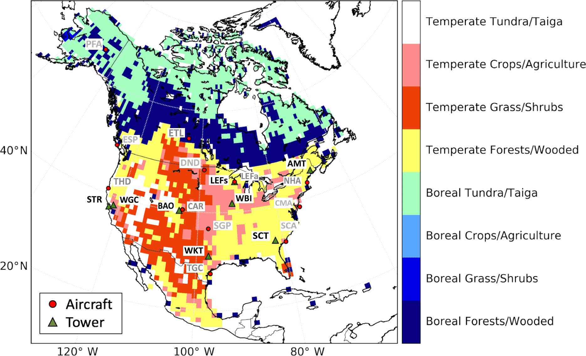
Figure 1 The model domain is shown together with the CO₂ observational sites from NOAA's Global Greenhouse Gas Reference Network and the aggregated Olson ecosystem types. Eight tall tower sites are highlighted by green triangles with black site code labels, and 12 selected aircraft sites are highlighted by red dots with gray site code labels.

2.1.1 Tall tower observations

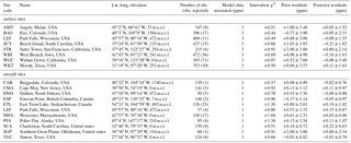
Table 1 Summary of assimilated PFP data from the NOAA ESRL North American tall tower and aircraft sampling program in 2010. We have selected 12 aircraft sites for this study. Observations (after data filtering, see Sect. 2.1.3) are flagged when the difference between simulated and observed values is larger than 3 times the prescribed model–data mismatch for each site. The bias indicates the mean difference between model forecast and observations.

Detailed site and sampling information of the tall tower observations is listed in Table 1. Andrews et al. (2014) used flask versus in situ comparisons for quality control and pointed out such comparisons suffer from quasi-continuous in situ data (due to, for example, switching of sampling lines among different heights, calibrations), difference in sampling time, and atmospheric variability. The mean differences between PFP and in situ CO₂ measurements over all eight sites for 2010 range from 0.08 to 0.32 ppm, with the standard deviation of the differences for each site ranging from 0.2 to 0.6 ppm and increasingly positive differences over the period 2008–2011. According to Andrews et al. (2014), the mean differences are likely caused by potential biases in an increasing number of the PFP measurements that may result from contamination caused by routine use throughout the network or by use under polluted conditions. A new flask sampling protocol was implemented in September such that the flask is pressurized with ambient air prior to sample collection and held at high pressure for several minutes then vented and resampled. Agreement has improved between flask and in situ measurement systems so the difference is reliably better than 0.2 ppm. We did not make any attempt to correct for the potential biases in the 2010 data. Masarie et al. (2011) shows that every 1 ppm of bias at Park Falls, Wisconsin, (labeled LEF) in the CarbonTracker inversion causes a linear response rate of 68 Tg C yr⁻¹ for temperate North American net flux estimates. However, if the bias is across the whole network, the impact on the net flux estimates will be much less than that.

2.1.2 Aircraft profiles

The NOAA ESRL aircraft CO₂ profile data (Table 1) are used to optimize lateral BCs. The aircraft program of the Global Greenhouse Gas Reference Network (Sweeney et al., 2015) has been collecting air samples for vertical profile measurements over North America since 1992. For each individual flight, 12 flask samples are collected from 500 m above ground up to 8000 m above sea level at most aircraft sites. Of the 15 ongoing aircraft sites by 2014, we have selected 12 sites (8 close to the domain boundary, and 4 in the middle of the domain) for this study. Because the aircraft program uses the same PFP flasks as in the tall tower program, the aircraft CO₂ measurements may have potential biases as well. Indeed, Karion et al. (2013) reported PFP minus in situ CO₂ measurements of 0.20±0.37 ppm for the aircraft measurements over Alaska from 2009 to 2011, a similar magnitude of biases as found in the tall tower PFP versus in situ comparisons.

2.1.3 Data filtering

We use daytime data from the tall towers that are collected between 10:00 and 18:00 local time to constrain surface fluxes. Aircraft observations made at altitudes higher than 3000 m above ground at all hours are used to constrain BCs. In CTDAS-Lagrange, we use fossil fuel emissions based on inventory estimates and do not attempt to optimize them. We remove CO₂ observations that are likely strongly influenced by fossil fuels before optimizing biosphere fluxes. This diminishes the potential biases in optimized biosphere fluxes that are caused by local fossil fuel sources and/or by representation errors in the simulated fossil fuel CO₂ signals. To achieve this, we use CO measurements as a proxy for fossil fuel influences, realizing that especially in summer other sources of CO can contribute to enhanced mole fractions. We first calculate CO enhancement as the difference between the CO observation and the background value, i.e., the corresponding value from a second order harmonic function that is fitted to the CO data for each tall tower site. We filter out any CO₂ observations with CO enhancements larger than 33.6 ppb, which corresponds to 3 ppm fossil fuel CO₂ according to the year-round median apparent ratio of 11.2 ppb ppm⁻¹, estimated in Miller et al. (2012). About 8.5 % of the available CO₂ data is excluded by the CO filter, with the majority coming from the two sites in California, labeled STR and WGC.

2.2 The CTDAS-Lagrange system

The CTDAS-Lagrange system aims to improve the estimates of regional carbon fluxes by combining a high spatial resolution Lagrangian modeling framework with the existing CarbonTracker Data Assimilation Shell (van der Laan-Luijkx et al., 2017). Transport of atmospheric CO₂ in the main application of CTDAS, the CarbonTracker Europe system, is realized by using the global two-way nested transport model TM5 (3^∘ × 2^∘ global, and 1^∘ × 1^∘ for one or more regional domains of interest) and driven by 3 h meteorological parameters. The CTDAS-Lagrange system replaces the coarse TM5 transport model with a Lagrangian transport model with high spatial resolution. Another advantage of the CTDAS-Lagrange system is its significantly improved time efficiency. Outputs from the Lagrangian transport model can be stored as measurement footprints (influence functions) so that the CO₂ mole fractions resulting from different surface flux configurations can be simulated offline afterwards, using simple matrix multiplications rather than full transport calculations. In addition, these stored outputs can be used for other species directly, significantly reducing the computation time when performing multiple or other species inversions, i.e., for the extension of our system to multi-species applications.

2.2.1 Atmospheric transport model

The Stochastic Time-Inverted Lagrangian Transport model coupled with the Weather Forecast and Research (WRF-STILT) is employed in our system (Lin et al., 2003; Nehrkorn et al., 2010). The STILT model is a receptor-oriented framework that links surface fluxes of trace gases with atmospheric mole fractions. During a WRF-STILT run, an ensemble of particles is released at the observation location (receptor) at a certain time, and particles are transported backward driven by the WRF wind fields. The influence function, i.e., footprint, for that particular receptor and time can be computed based on the density of the particles in the surface layer defined in STILT as the lower half of the well-mixed boundary layer (Gerbig et al., 2003).

We leverage a footprint library created for the NOAA CarbonTracker Lagrange regional inversion framework (https://www.esrl.noaa.gov/gmd/ccgg/carbontracker-lagrange/, last access: 25 August 2018). The WRF-STILT model was run with 500 particles that are traced backward for 10 days. The WRF model (version 3.3.1 for the 2010 time period of this study) was configured with a Lambert conformal map projection to cover continental North America, with a spatial resolution of 10 km for the inner domain over the continental US (∼25–55^∘ N; 135–65^∘ W) and 40 km for the outer domain (∼10–80^∘ N; 170–50^∘ W), and 40 vertical layers, which is similar to the configurations in Nehrkorn et al. (2010) and Hu et al. (2015). The North American Regional Reanalysis (Mesinger et al., 2006) provided initial and lateral BCs. Model runs were initialized every 24 h, with the initial 6 h of each 30 h forecast discarded to allow for model spin-up. Species-independent 10-day surface footprints with 1^∘ × 1^∘ spatial resolution and hourly time resolution are computed with STILT and stored for each measurement along with back-trajectories. Snapshots of the 3-dimensional particle distribution are also stored to enable assignment of boundary values according to where particles intersect with the domain of the inversion.

2.2.2 Optimization scheme

In the CTDAS-Lagrange system, we extended the existing ensemble Kalman smoother method as is implemented in CarbonTracker and CarbonTracker Europe (Peters et al., 2005, 2007, 2010; van der Laan-Luijkx et al., 2017) to simultaneously optimize biosphere fluxes and BC parameters.

We use two alternative ways of adjusting the total surface fluxes (additive and multiplicative), while simultaneously optimizing the lateral BCs by optimizing four parameters that are implemented as follows:

$$\begin{array}{ll}{\displaystyle }& {\displaystyle }C\left(X_{\mathrm{r}},t_{\mathrm{r}}\right)=C_{\mathrm{0}}\left(X_{\mathrm{r}},t_{\mathrm{r}}\right)+{\sum }_{i=\mathrm{0}}^{\mathrm{4}}{W}_i\left(X_{\mathrm{r}},t_{\mathrm{r}}\right)\cdot {\mathit{\beta }}_i\\ \text{(1)}& {\displaystyle }& {\displaystyle }+S\left(X_{\mathrm{r}},t_{\mathrm{r}}\mathrm{|}x,y,t\right)\cdot \left\{\begin{array}{l}f\left[\mathit{\lambda },F_{\mathrm{bio}}\left(x,y,t\right)\right]\\ F_{\mathrm{ff}}\left(x,y,t\right)\\ F_{\mathrm{ocn}}\left(x,y,t\right)\\ F_{\mathrm{fire}}\left(x,y,t\right)\end{array}\right\},\end{array}$$

where C(X_r,t_r) is the simulated CO₂ mole fraction (ppm) at the location of the observation (receptor) X_r and time t_r; C₀(X_r,t_r) refers to the contribution of advection from the lateral BC (ppm); β_i (ppm) is adjusted to optimize the lateral BC for each of the four sides of the regional domain for each 10-day period. The BC mole fraction β_i is weighted by the pre-calculated coefficient W_i(X_r, t_r) (unitless) that is determined as the ratio of the number of particles exited from one side of the domain to the number of particles exited from all sides of the domain. The domain considers 3000 m as the top boundary, which means that the particles that exited the domain below 3000 m, or did not leave the domain within 10 days, were not used to calculate the weight W_i(X_r, t_r). In case all particles left the domain below 3000 m, the weights of BC parameters were zero and the BC was not adjusted. This choice reflects the dominant influence of surface fluxes over lateral advection for particles that spent considerable time within the inner domains. $S\left(X_{\mathrm{r}},t_{\mathrm{r}}\mathrm{|}x,y,t\right)$ is the footprint – sensitivity of mole fraction variations to surface fluxes, ppm (µmol m⁻² s${}^{-\mathrm{1}}{)}^{-\mathrm{1}}$ – calculated with STILT. Biosphere fluxes $F_{\mathrm{bio}}(x,y,t)$ (µmol m⁻² s⁻¹) are optimized by either additively or multiplicatively optimizing a set of parameters λ (µmol m⁻² s⁻¹, or unitless) for each 1×1^∘ grid in the domain for each 10-day period, represented by the function f[$\mathit{\lambda },F_{\mathrm{bio}}(x,y,t)$] in the equation. $F_{\mathrm{ocn}}(x,y,t)$, $F_{\mathrm{ff}}(x,y,t)$, and $F_{\mathrm{fire}}(x,y,t)$ denote the CO₂ fluxes (µmol m⁻² s⁻¹) exchanged with ocean, from fossil fuels and fires, and these are fixed.

The state variables therefore include the gridded adjusting parameters for the biosphere fluxes (3078 land grids with $\mathrm{1}{}^{\circ }\times \mathrm{1}$^∘ resolution over North America) plus those for the four BC parameters, leading to a total of 3082 parameters for each 10-day period. The state variables are optimized simultaneously within each period. Considering that aircraft observations above 3000 m mostly contain information about BCs and have low or even no sensitivity to surface fluxes, we optimize the biosphere fluxes using tower observations only, and optimize BCs with both tower and aircraft observations. This separation is applied through localization of the Kalman gain matrix.

2.2.3 System setup

The system aims to optimize (non-fire) net ecosystem exchange (NEE) of CO₂ between biosphere and atmosphere, and requires prior biosphere fluxes, lateral BCs, and other fixed fluxes such as fossil fuel emissions and ocean and fire fluxes as model input. This section describes the setup of the base case run.

We use biosphere fluxes simulated by the combined Simple Biosphere and Carnegie-Ames-Stanford Approach (SiBCASA) model (Schaefer et al., 2008) as a prior and fixed fossil fuel burning, ocean, and fire fluxes from CT2013B (Peters et al., 2007, with updates documented at http://carbontracker.noaa.gov, last access: 25 August 2018) with the latter two being negligibly small in the annual mean over our domain of interest, but still included since they introduce spatiotemporal variations in CO₂ mole fractions. More details about these prior and the component fluxes are described in Sect. 2.2.4. The lateral BC is also taken from the 4-D mole fraction fields simulated by CT2013B. We use the WRF-STILT transport model. Here we give a short summary of the configuration of the base case run: we prescribe an additive biosphere fluxes uncertainty of 1.6 µmol m⁻² s⁻¹; a prior uncertainty in the BC parameters of 2.0 ppm, a model–data mismatch of 3 ppm for surface sites and 1 ppm for aircraft sites, and a covariance length scale of 750 km.

We estimate the additive flux adjustments for each grid box in our domain, but a covariance structure is used to reduce the number of degrees of freedom in the state vector, and to balance it with the number of available observations. The covariance is calculated as an exponential function that decreases with distance between grid boxes, using a decorrelation length scale of 750 km. This covariance is only used between grid boxes that have the same dominant plant-functional type, as specified though the ecoregion maps that are also used in CT2013B. These in turn are based on TransCom regions, as well as the Olson ecosystem classification (Olson et al., 2002). Where CT2013B uses single scaling factors for each ecoregion, our gridded approach has approximately 122 degrees of freedom within its 3078 additive adjustment parameters as compared to an average of 112 independent observations per assimilation time step.

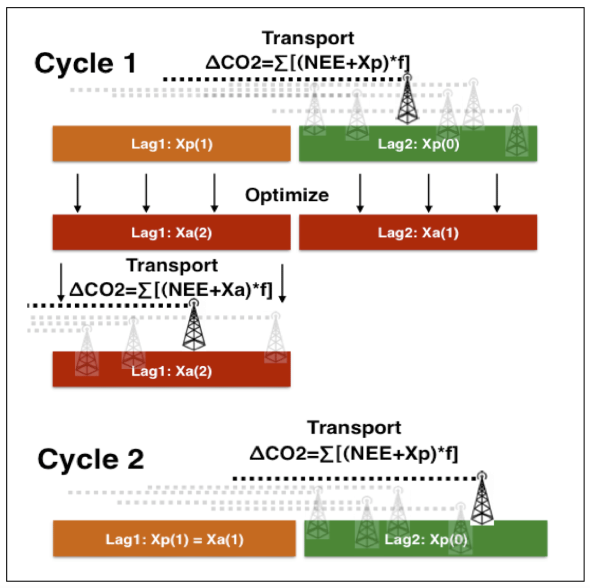
Figure 2 The time stepping flow of the ensemble Kalman smoother filter used in CTDAS-Lagrange. The Xp(n) and Xa(n) represent the prior and optimized state vector of a 20-day period shown as two colored bars from left to right. Parameter n denotes the number of times the state vector has been updated. Each of the colored bars represents a “lag” of 10 days. In the transport step we calculate the CO₂ mole fraction variations (ΔCO₂) for each measurement (shown as a tower) by convolving the net biosphere flux NEE + Xp∕Xa with footprints f (shown as a dashed line). Cycle 1 starts by introducing a new set of observations and fluxes at the front of the filter in lag 2. This part of the state vector has not been optimized before (green color, n=0). At the rear end of the filter, in lag 1, the state vector has been optimized once in the previous cycle (orange color, n=1). To estimate ΔCO₂ for each observation requires convolving footprints with 10-day 3-hourly NEE + Xp. Optimization is done on all 20 days (2 lags of the filter) to find the optimal values in the entire state vector. The state vector of lag 1 is done and will not change again (red color, n=2). This new optimized state vector Xa(2) is used to calculate the final ΔCO₂ in lag 1 (final transport step). Cycle 2 starts by introducing a new set of observations and fluxes at the front of the filter in lag 2. The analyzed state vector Xa(1) in lag 2 of Cycle 1 becomes the new prior state vector Xp(1) in lag 1 of Cycle 2.

We have adapted the fixed lag ensemble Kalman smoother method from Peters et al. (2005) to estimate fluxes and BC per 10-day time step. Because the footprint of each receptor can go back in time up to 10 days, we need a total assimilation window of 20 days to account for the backward trajectories that overlap two time steps. Therefore, the total state vector contains flux and BC parameters for two 10-day time steps (3082×2). The time stepping cycle works as follows (see Fig. 2): First, we use an ensemble of parameters derived from the total state vector to calculate an ensemble of modeled CO₂ mole fractions for each measurement extracted in the current 10-day time step. These state vector parameters reflect the influence of fluxes and BCs on the modeled CO₂ in the current 10-day time step and the previous 10-day time step that has already been optimized once in the previous cycle. In the next step, the set of ensemble Kalman smoother equations as outlined in Peters et al. (2005) is solved to give a new set of optimized state vector parameters and its ensemble, where the state vector of the previous time step is optimized for a second and final time. Modeled CO₂ from the previous time step is updated using the final state vector. Finally, the next cycle starts 10 days forward in time by introducing a new set of measurements. In this way, each 10-day state vector is finalized after two cycles of optimization.

A comparison of the setup between the base case and sensitivity runs (described in the Sect. 2.3) is given in Table 2.

Table 2 Summary of the base and sensitivity runs using CTDAS-Lagrange.

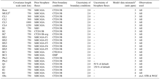
¹ Here shows the model–data mismatch for tower observations. A model–data mismatch of 1 ppm is used for aircraft observations in all simulations;
² Indicates the run uses a multiplicative method for flux adjustment.

2.2.4 Prior biosphere and other fluxes

The prior biosphere fluxes are simulated by the SiBCASA model, a diagnostic biosphere model, which combines photosynthesis and biophysical processes from the Simple Biosphere (SiB) model version 3 with carbon biogeochemical processes from the Carnegie-Ames-Stanford Approach model (Schaefer et al., 2008). Meteorological driver data are provided by the European Centre for Medium-Range Weather Forecasts (ECMWF). SiBCASA calculates the surface energy, water, and CO₂ fluxes at a 10 min time step on a spatial resolution of 1^∘ × 1^∘, and predicts the moisture content and temperature of the canopy and soil (Sellers et al., 1996). SiBCASA uses one of the 12 dominant biome types at 1×1^∘ resolution. But it does include the distinction of C₃ and C₄ photosynthesis using the C₄ coverage map from Still et al. (2003), which means that the grid cells contain a fraction of both C₃ and C₄ plant types, and the carbon uptake is computed separately from each of the plant types. We use the 3-hourly mean CO₂ fluxes as is used in van der Velde et al. (2014) and van der Laan-Luijkx et al. (2017).

CT2013B offers a number of flux estimates (ocean, fossil fuels, etc.) from multiple models, which includes two different flux datasets for ocean and fossil fuels, respectively. The fire fluxes are based on the Global Fire Emissions Database (GFED) 3.1, which are calculated with the CASA model (Giglio et al., 2006; van der Werf et al., 2006). The fire fluxes are not optimized in CT2013B. The two different prior ocean fluxes for CT2013B include a long-term mean of ocean fluxes that is derived from the ocean interior inversions (Jacobson et al., 2007) and a climatology dataset that is created from direct observations of seawater around the world and was interpolated onto a regular grid map using a modeled surface current field (Takahashi et al., 2009). We use the optimized ocean fluxes of CT2013B that are calculated as the mean of an ensemble of run results. The two different fossil fuel fluxes for CT2013B are the “Miller” emissions dataset and the “ODIAC” emissions datasets (Oda and Maksyutov, 2011). The difference between the two datasets is the processing schemes on the totals and the spatial and temporal distributions of fossil fuel emissions. The fossil fuel fluxes are not optimized in CT2013B. We use the fixed fossil fuel data of CT2013B, which is an average of “Miller” and “ODIAC”. The final product of these fluxes is provided on 1^∘ × 1^∘ grid at a 3-hourly temporal resolution. More details can be found at the CarbonTracker website CT2013B (https://www.esrl.noaa.gov/gmd/ccgg/carbontracker/CT2013B/index.php, last access: 25 August 2018).

2.3 Sensitivity runs

2.3.1 Lateral boundary conditions (BCs)

The lateral BCs could be constructed either from interpolated measurements or from the output of a global tracer model. The base case uses CT2013B optimized mole fraction fields.

To study the impact of different lateral BCs on flux optimization, we have tested optimized mole fraction fields with the spatial resolution of 1^∘ × 1^∘ from CarbonTracker Europe (CTE2014), as well as empirical (EMP) background mole fraction fields. Pacific marine boundary layer data from the NOAA Earth System Research Laboratory's Cooperative Air Sampling Network and vertical profile data from aircraft were used to produce a background mole fraction field varying across latitudes, altitudes, and time. This three-dimensional background “curtain” represents mole fractions of CO₂ in the remote atmosphere between 10 and 80^∘ N and from 0 to 7500 m a.s.l. It was derived using the same curve-fitting algorithms described in Masarie and Tans (1995). Similar background fields have been used in regional inverse-modeling studies of CH₄, CO₂, and other gases (e.g., Gourdji et al., 2012; Jeong et al., 2013; Miller et al., 2013; Hu et al., 2015). Similarly, the lateral BC was constructed in Gerbig et al. (2003) based on a series of analytical functions, which were used to fit measurements at selected ground stations and from aircraft data from various campaigns.

We also assign different prior uncertainties other than 2 ppm for the BC parameters. Experiments are designed as follows:

• BC1: using CTE2014 mole fraction fields as lateral BCs;

• BC2: using EMP as lateral BCs;

• Pbc1: set the uncertainty in the BC parameter to 1 ppm;

• Pbc2: set the uncertainty in the BC parameter to 3 ppm.

For all other aspects, the model is configured to be identical to the base case run.

2.3.2 Prior biosphere fluxes

Gurney et al. (2004) point out that inversion results can be sensitive to a priori fluxes for regions with sparse observations while the fluxes can be well constrained by areas with dense observations. To investigate the impact of different a priori fluxes on the optimized fluxes, we have designed two sensitivity runs that incorporate two alternative biosphere fluxes as a priori fluxes as follows:

• B1: SiB3 biosphere fluxes;

• B2: CT2013B optimized biosphere fluxes.

Except for the difference in the a priori biosphere fluxes, the two sensitivity runs share the same model setup as the base case. SiB3 biosphere fluxes are the simulation results of the third version of the Simple Biosphere model (Baker et al., 2008), with hourly fluxes and a spatial resolution of 1^∘ × 1^∘. CT2013B optimized biosphere fluxes are the outputs of CT2013B that optimizes the global surface biosphere fluxes, which uses higher-resolution transport over North America than other regions. Although these fluxes are already optimized against global and North American CO₂ observations, it is still interesting to optimize them in a different assimilation system, especially when the system employs a high spatial resolution and different transport model. In addition, CT2013B assimilates a different set of observations compared to CTDAS-Lagrange. In principle, one expects these fluxes to be most consistent with observations, and to lead to a very similar posterior mean flux as was prescribed through the prior.

For further analysis of the sensitivity of the CTDAS-Lagrange system to the annual mean and the seasonal magnitude of a priori fluxes, we have designed a series of runs with modified SiBCASA fluxes. We scaled the respiration of the SiBCASA fluxes while maintaining the gross primary production (GPP) estimate to obtain a priori North American annual mean fluxes ranging from +0.43 to −2.06 PgC yr⁻¹. The tests with prior fluxes +0.43, −0.06, −0.97, −1.44, and −2.06 PgC yr⁻¹ are labeled with BX1, BX2, BX3, BX4, and BX5, respectively.

2.3.3 Additive or multiplicative flux adjustment

The multiplicative flux adjustment of NEE relates the uncertainties to the magnitude of the fluxes. As NEE is the difference between two gross fluxes, gross primary production and ecosystem respiration, 10-day mean NEE can be very small or even close to zero when GPP and respiration are close to each other, e.g., in the so-called shoulder seasons (see Fig. 8), which limits the ability of using multiplicative flux adjustment to scale the mean fluxes due to low uncertainties in the inversion system (note that the large diurnal cycle of the net flux will still be scaled though). Scaling both GPP and respiration has been shown to circumvent this in deriving optimized mean fluxes (Tolk et al., 2011). Here, we have instead implemented both multiplicative and additive flux adjustment methods. For the multiplicative method, we set the biosphere scaling parameter variance as 80 %, following Peters et al. (2010); for the additive method, the variance is prescribed as 1.6 µmol m⁻² s⁻¹ which represents the typical flux uncertainty in the multiplicative method during the summer months. Because this value persists yearlong in the additive run, the total annual uncertainty in this method is higher though. Sensitivity tests for the covariance are described below. The additive method is used in the base case run, and the multiplicative method was tested as a sensitivity run.

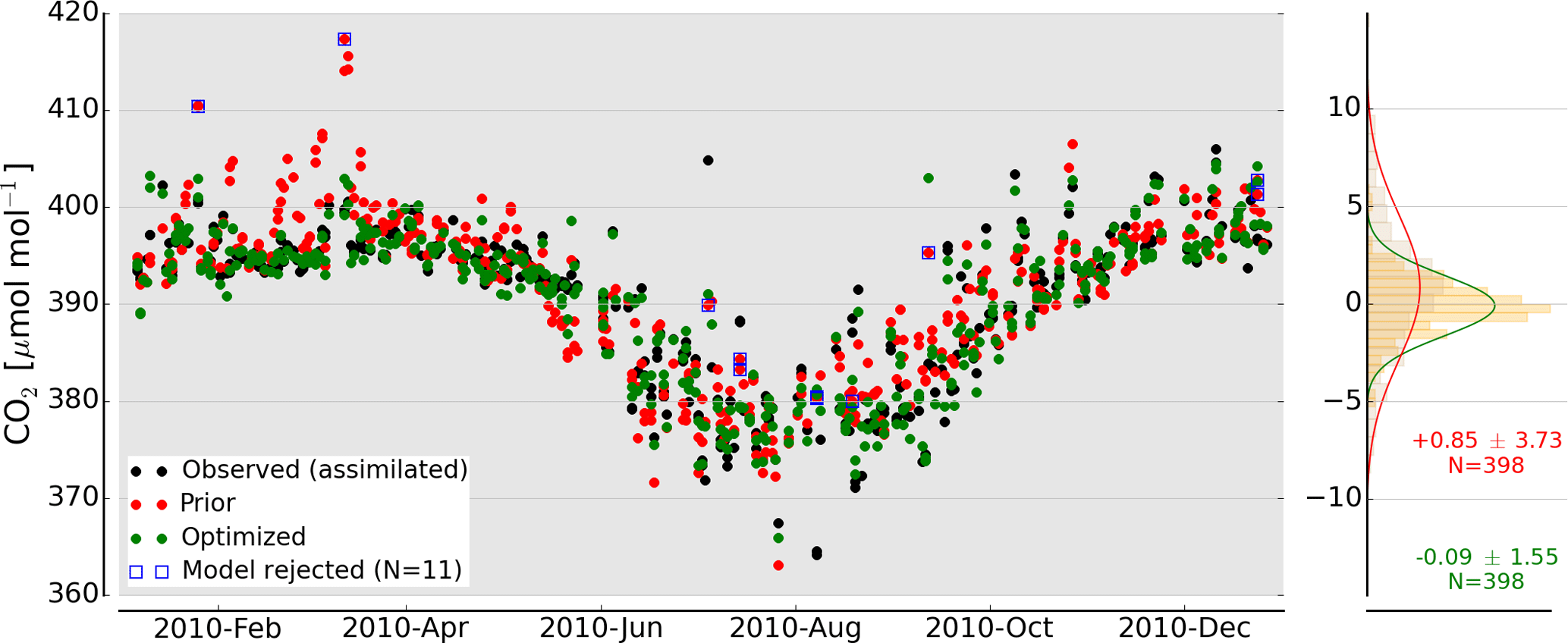
Figure 3 Simulated CO₂ (prior in red and optimized in green) and observed CO₂ (black) for the Park Falls, Wisconsin, tower site (labeled LEF) for the year 2010. The blue squares (11 out of 409 samples) are rejected samples because the difference between simulated and observed CO₂ is larger than 3 times the assigned model–data mismatch of 3 ppm for tower sites. The distribution of both prior and posterior residuals is presented on the right side. After optimization we observe a strong reduction of the CO₂ mean bias and 1σ standard deviation from $+\mathrm{0.85}\pm \mathrm{3.73}$ to $+\mathrm{0.09}\pm \mathrm{1.55}$ ppm. Note that the prior residual distribution is calculated without the rejected observations, which explains the slightly different statistics in comparison to the data presented in Table 1.

For a better assessment of the adjusting ability of the two methods, we further perform experimental inversions using pseudo-data, i.e., Observing System Simulation Experiments (OSSEs). The primary aim of our OSSEs is to investigate the ability of our system to retrieve surface fluxes given the observational network. In particular, we test the implementation of the additive flux parameter vs. multiplicative flux parameter, and the ability to recover large biases in lateral BCs and prior fluxes. We run the CTDAS-Lagrange in a forward mode with the SiBCASA fluxes as prior to generate simulated mole fractions, and then try to recover the “truth” in an inversion using SiB3 fluxes as a priori.

2.3.4 Covariance length scales

The covariance length scale determines the rate at which the correlation between the fluxes of two grids within the same ecoregions decreases exponentially with increasing distance. The prescribed covariance effectively reduces the number of unknowns to be solved for, and improves the ability of the inversion system to retrieve optimized fluxes when data are limited (Rödenbeck et al., 2003; Gourdji et al., 2012). The choice of appropriate correlation length scale depends also on the observation density. For example, CarbonTracker Europe, which includes more observations than those used in this work, uses a correlation length scale of 300 km for North America. In addition, Alden (2013) found 700 km to be the best length scale to recover true fluxes over North America with a pseudo-data inversion experiment. To investigate the impact of covariance length scales on optimized fluxes, we performed sensitivity runs with a series of spatial correlation lengths: 300, 500, 750 km (base case), 1000, and 1250 km, labeled as CL1 to CL4, respectively.

2.3.5 Magnitude of covariance and model–data mismatch

Flux covariance determines the range in which prior biosphere fluxes can be adjusted. It should ideally reflect the uncertainty in prior biosphere fluxes, but information about prior flux errors is not readily available for the priors used here or for terrestrial ecosystem models more generally. To evaluate the possible influence of prior covariances on the optimized fluxes, we modified the additive uncertainty by ±50 %. The model–data mismatch (MDM) is a parameter that describes the capability of our modeling system to match the observations, and is used to de-weight observations that are not well represented by the model simulations, e.g., in the case of local influence. The observations are even excluded when the differences between observed and simulated CO₂ are larger than 3 times the MDM. We set the MDM to 3.0 ppm for tower sites and 1.0 ppm for aircraft sites. The sensitivity tests that incorporate the covariance and MDM are described below:

• Q1: decrease the magnitude of additive uncertainty by 50 %, which means the covariance is 25 % of the default;

• Q2: increase the magnitude of additive uncertainty by 50 %, which means the covariance is 225 % of the default;

• R1: set the MDM to 2 ppm for tower sites;

• R2: set the MDM to 4 ppm for tower sites.

The rest of the model setup is the same as the base case run.

2.3.6 Observational data choice

As a sensitivity test, we exclude observations at two tower sites (STR and WGC), which are characterized with larger prior and posterior residuals (simulated minus observed, both mean and standard deviation) than other sites. We have defined one sensitivity run as follows:

Obs: excluding STR and WGC, and the rest of the model setup is the same as the base case run.

3 Results

This section covers the following topics: CO₂ mole fraction simulations and seasonal cycles of biosphere fluxes from the base case run, lateral BCs choice and optimization, sensitivity to a priori fluxes, additive or multiplicative adjusting parameters, covariance length scales, transport uncertainties, and a summary of ensemble estimates.

3.1 Observed and simulated CO₂ mole fractions

As an example, a time series of simulated and observed CO₂ mole fractions at the LEF tower site for the year 2010 is shown in Fig. 3. As should be expected from the assimilation, the optimized CO₂ records closely follow the CO₂ observations over time, and the optimized residuals (green) are smaller than those from the model forecast (red). The distribution of both prior and posterior residuals shown on the right side of Fig. 3 indicates improvement from the prior $+\mathrm{0.85}\pm \mathrm{3.73}$ ppm to the posterior 0.09±1.55 ppm. The larger variability in both observed and simulated CO₂ between May and November (compared to the rest of the year) are likely caused by larger variability in the biosphere fluxes during the growing season, as well as larger variation in atmospheric mixing conditions. A few simulated values (blue) are rejected in the assimilation procedure because the difference between simulations with prior biosphere fluxes and observations is larger than 3 times the assigned model–data mismatch of 3 ppm for tower sites. For the LEF tower site, 11 out of the total 409, or 2.9 % are rejected, which is slightly larger than the expected rejection rate (based on a 3σ cut-off for a Gaussian probability density function of the errors) of 2 % (Peters et al., 2010). It is shown in Table 1 that the rejection rates for most tower sites are around 2–3 %, except for WBI (7.6 %) and WGC (18.0 %).

3.2 Seasonal cycles of net ecosystem exchange (NEE) of CO₂

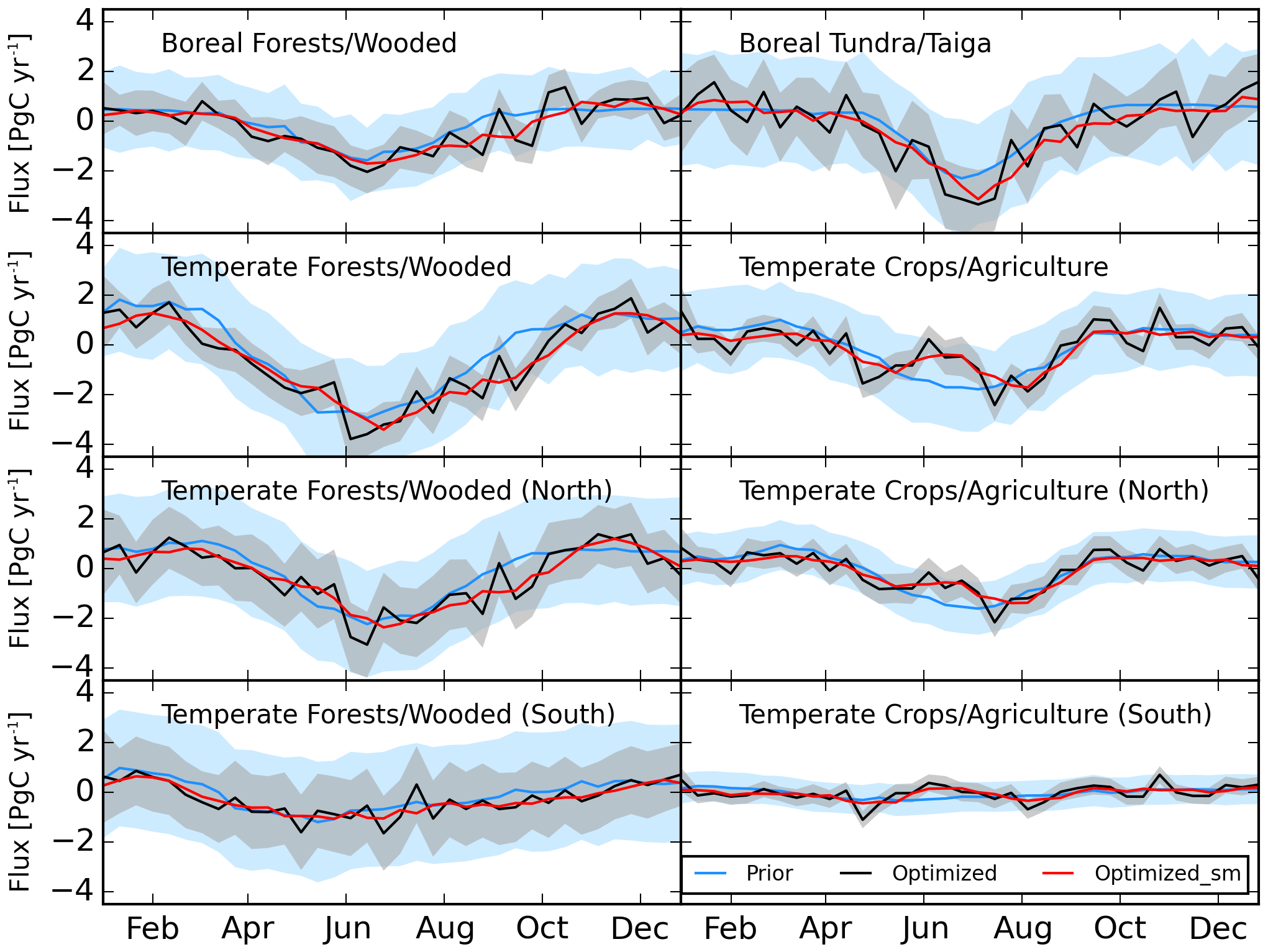
Figure 4 The seasonal cycle (10-day resolution) of the net CO₂ biosphere flux (PgC yr⁻¹) of four aggregated Olson ecoregions in North America for the year 2010. The prior biosphere flux (SiBCASA) and its uncertainty are displayed in blue, and the optimized biosphere flux and uncertainty in black. “Optimized_sm” stands for the smoothed optimized fluxes (shown in red), which helps to remove the spurious fluctuations. The Temperate Forests/Wooded and Crops/Agriculture are separated by 40^∘ N into North and South, respectively.

Figure 4 shows the seasonal cycle (10-day averages) of NEE of CO₂ for the year 2010 for four major Olson aggregated land-cover types of North America (Boreal Forests/Wooded, Boreal Tundra/Taiga, Temperate Forests/Wooded, and Temperate Crops/Agriculture). The amplitude of the seasonal cycle of temperate forests/wooded is the largest among the four land-cover types, with both large summertime vegetative uptake and large wintertime respiratory emissions. Since the same ecoregions may correspond to multiple regions and climates, we have separated the southern and northern regions for crops and forests (divided by 40^∘ N). The seasonal cycles are mainly caused by those in the northern regions, especially for crops. The uncertainties in the posterior fluxes have been reduced for all four land-cover types and for almost all seasons of the year, especially for temperate forests/wooded and temperate crops/agriculture.

The seasonal cycle of the posterior fluxes shows a similar magnitude as the prior. In addition, the optimized fluxes generally show more fluctuations than prior fluxes over the year, which could be explained by effective constraints from atmospheric observations and possibly in some cases as artifacts that are caused by the sparseness of the observations. It should be noted that it does not mean that the actual errors in these fluxes are really reduced, as this can only be assessed using independent observations of these fluxes. With monthly averaging, the fluctuations in the derived posterior fluxes could be significantly reduced (see Fig. 4). Interestingly, the temperate crops/agriculture show double troughs in the uptake in May and July–August or a sudden drop in the uptake in June, which could be attributed to early-summer crops/agriculture harvests, temperature anomaly, or drought.

The mean prior and optimized fluxes for the summer months June–August are given in Fig. 5. The optimized fluxes show a similar spatial pattern as the prior fluxes, but display more spatial details. The optimized results place more carbon uptake in the agricultural US Midwest and the forests/wooded in the northeast of the US, as well as in the boreal forests/wooded and tundra/taiga of Canada; In contrast, less carbon uptake (or carbon emissions) is placed in the western US, especially in south Utah, north Arizona, and Louisiana.

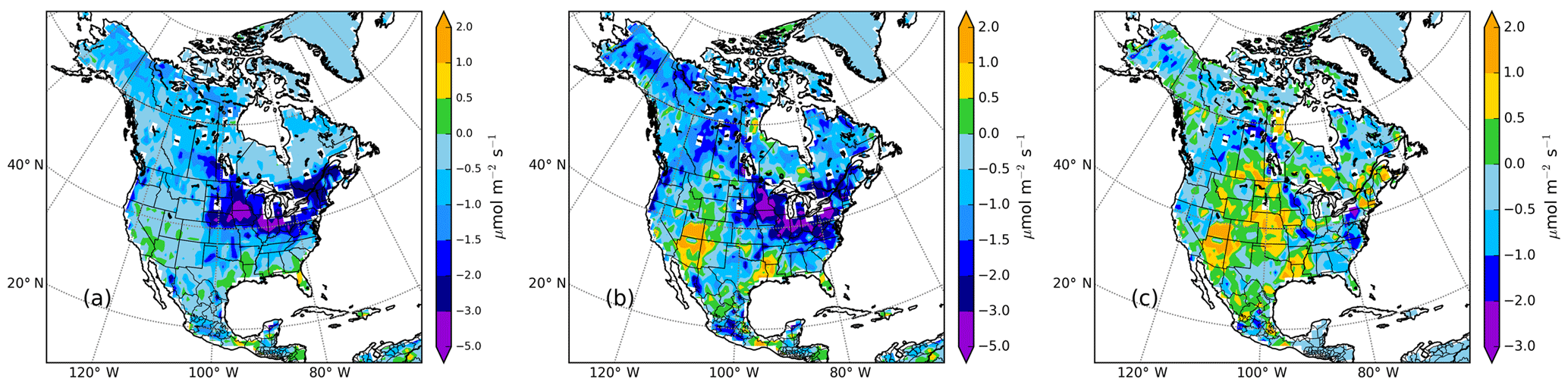
Figure 5 Mean prior (a) and optimized (b) net biosphere fluxes, and the mean adjustment (optimized minus prior) (c) for summertime (June–July–August). Note that the color scale used in (c) is different from the one used in (a) and (b).

3.3 Boundary condition choice and optimization

Table 3 Contribution of lateral transport to simulated CO₂ mole fractions at the tall tower network for three sets of lateral BCs. The mean differences (in ppm) between CTE2014, EMP, and CT2013B BCs are calculated for 2010 and summer (JJA), respectively. The standard deviation (1σ) of the differences for each tower site is given in the parenthesis.

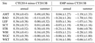
A comparison of the mole fraction contribution from three lateral BCs for the eight tower sites is summarized in Table 3. The annual means of the CTE2014 are consistently ∼0.30 ppm higher than those of the CT2013B for all sites; however, the summertime means of the CTE2014 and the CT2013B are nearly equal except for the two sites AMT and STR. In contrast, the annual means of the EMP and the CT2013B are nearly equal for all sites; however, the summertime drawdowns of the EMP are significantly higher (−1.70 to −0.28 ppm) than those of the CT2013B for all sites except STR (0.66 ppm). This suggests that the two model-derived BCs provide higher summer background mole fractions than the EMP-based background, which corresponds to a known high bias in summertime CO₂ across North America in both versions of CarbonTracker used to construct the BCs.

Table 4 Comparison of the optimized annual net biosphere fluxes (PgC yr⁻¹) and the adjustment of CO₂ boundary conditions (BCs, ppm) using different prior lateral BC products (CT2013B, CTE2014, and EMP) and optimization techniques (“Flux only” or “Flux+BC”). The annual net biosphere flux difference is calculated from the “Flux+BC” optimization minus “Flux only” optimization. The values in brackets are flux uncertainties.

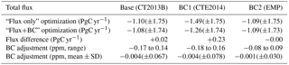
The optimized annual mean fluxes and the adjustment of the BC parameters for the model runs with different prior lateral BCs are shown in Table 4. When both biosphere fluxes and BC parameters are optimized, i.e., “Flux+BC” optimization, the optimized annual mean fluxes using three different prior lateral BCs range from −1.26 to −1.08 PgC yr⁻¹, with an average of $-\mathrm{1.14}\pm \mathrm{0.10}$ PgC yr⁻¹, which have a smaller variation compared to those from the model runs when only biosphere fluxes are optimized, i.e., “Flux only” optimization, that ranges from −1.49 to −1.09 PgC yr⁻¹ or $-\mathrm{1.22}\pm \mathrm{0.23}$ PgC yr⁻¹ (discussed in more detail in the following section). The results show that the additional BC optimization is desired when model-based BCs are used, and that this reduces the annual mean optimized biosphere fluxes by up to 0.23 PgC yr⁻¹, or 15.4 % of the “Flux only” optimized fluxes. The largest adjustment in the optimized annual mean biosphere uptake takes place in the run with the CTE2014 as lateral BCs, which corresponds to the consistently higher annual means of the BC contributions of the CTE2014 than those of the CT2013B. The contribution of the adjustment of BC parameters to simulated CO₂ ranges from −0.18 to 0.16 ppm over all seasons of the year 2010, which stresses that this is a subtle, but systematic, signal to account for in a regional inversion.

The residuals of the model runs with and without BC optimization (not shown), in almost all cases, are significantly reduced after optimization. The reduction in the residuals after optimization for aircraft sites is primarily due to the adjustment of the BC parameters. We notice that the residuals (means and standard deviations) of the model runs with optimized biosphere fluxes and BC parameters for the two sites STR and WGC are larger than those for other sites. Possible reasons are that the two sites are still significantly influenced by regional fossil fuel signals after the data filtering presented in Sect. 2.1.3, and are less sensitive to biosphere fluxes (due to their proximity to the west coast of North America there is less sensitivity to land flux than for other sites). We will investigate the impact of the two observation sites on optimized fluxes in the following section.

The time series of optimized North American averaged biosphere fluxes from the model runs with different prior lateral BCs are shown in Fig. 6. The differences among the optimized fluxes with additional BC optimization (Fig. 6b) become smaller than those from the “Flux only” runs (Fig. 6a). This can also be observed when averaged over major ecoregions (Fig. 6c and d), especially for the boreal forests and temperate forests. The differences in the optimized biosphere fluxes caused by different prior lateral BCs are mostly small, except that the deviation of the EMP optimized fluxes from the other two is slightly larger for the period July–September.

Figure 6 Mean optimized net biosphere fluxes (PgC yr⁻¹) for the runs with different prior boundary conditions (BCs): CT2013B, CTE2014, and EMP. The time series of optimized fluxes are presented for the “Flux only” inversion (a) and for the “Flux+BC” inversion (b), respectively; the annual net biosphere fluxes over the aggregated Olson ecosystem types are shown for the “Flux only” inversion (c) and for the “Flux+BC” inversion (d), respectively. Note that in panels (c) and (d) the first letters “B” and “T” of the x-axis labels are short for “Boreal” and “Temperate”, respectively; the second letters “F”, “G”, “C”, and “T” are short for ecosystem types “Forests/Wooded”, “Grass/Shrubs”, “Crops/Agriculture”, and “Tundra /Taiga”, respectively.

3.4 Sensitivity to prior biosphere fluxes

Table 5 Optimized annual net biosphere fluxes (PgC yr⁻¹) and CO₂ boundary condition (BC) adjustments (ppm) using four prior biosphere flux products (SiBCASA, SiB3, CT2013B, and CT2013B-avg). The values in brackets are flux uncertainties.

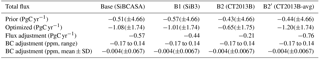
The optimized annual mean biosphere fluxes and associated BC parameter adjustments from the runs with different prior biosphere fluxes are shown in Table 5. The flux adjustments are in general large, resulting in significantly larger annual mean uptake over North America than the prior; however, the optimized annual mean fluxes from the runs using three different prior biosphere products converge, except for the run using the original CT2013B optimized fluxes. A further check indicates that the residuals of the run are reasonable, but more observations have been rejected compared with the other runs. The rejection takes place in the period from June to August, which is caused by large fluctuations of the a priori fluxes. Note that the a priori CT2013B fluxes are optimized using weekly scaling factors in an assimilation window of 5 weeks long and incur substantial variability (or noise) that averages out over larger scales in CT2013B. But the forward simulations of the CTDAS-Lagrange system are sensitive to the fluxes and their diurnal cycle is only in a 10-day window and therefore more sensitive to this variability (or noise). Therefore, we have made an additional sensitivity test (B2^′) with smoothed CT2013B fluxes (10-day averaged, identical 3-hourly fluxes across a day in every 10-day period) as a priori, which gives smaller optimized annual fluxes (see Table 5). Because the prior CT2013B fluxes contain large fluctuations, we have averaged the fluxes within 10-day windows to a single constant value. We are fully aware that this is not realistic, and this should be regarded as a sensitivity test to understanding the difficulties of our CTDAS-Lagrange system to high-frequency fluctuations in the prior fluxes with limited flexibility (prior flux uncertainty). We hereafter refer to CT2013B-avg for further analysis.

Figure 7a shows the time series of the North American averaged biosphere fluxes of the model runs with different prior biosphere fluxes. It is noticeable that the difference in the seasonal amplitude between the SiB3 prior biosphere fluxes and the other two prior biosphere fluxes is diminished after optimization. Furthermore, the significant difference among the three prior products for the period August–October is largely reconciled by the inversion. Annual mean fluxes per ecoregion (Fig. 7c) indicate that the largest adjustment in the fluxes takes place for temperate forests and temperate grass, with fluxes from temperate grass changed from uptake to emissions. Note that the optimized fluxes per ecoregion do not always agree on their magnitudes, which is likely caused by insufficient constraints by observations, especially for the boreal region.

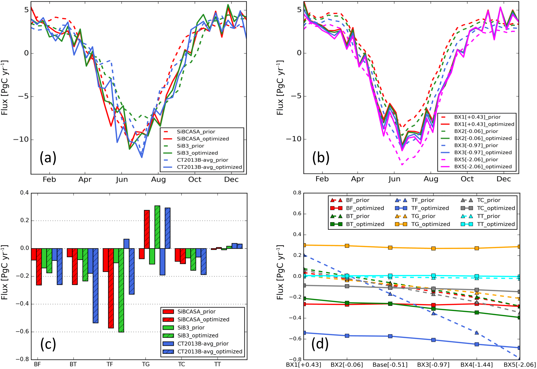
Figure 7 Prior and optimized annual net biosphere fluxes (PgC yr⁻¹) for North America for the runs using different prior biosphere model products: (a) SiBCASA, SiB3, CT2013B-avg, and (b) a series of modified SiBCASA fluxes derived from scaling up and down respiration fluxes. The time series of the optimized fluxes for both cases are presented in (a) and (b), respectively, and the annual net biosphere fluxes aggregated per ecoregion are accordingly presented in (c) and (d), respectively. The tests with prior fluxes +0.43, −0.06, −0.97, −1.44, and −2.06 PgC yr⁻¹ are labeled with BX1, BX2, BX3, BX4, and BX5, respectively.

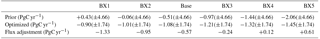
To further investigate the sensitivity of the CTDAS-Lagrange system to the seasonal magnitude and the annual mean of a priori fluxes, we scale the respiration of the SiBCASA fluxes to obtain a variety of a priori fluxes with the annual mean NEE ranging from +0.43 to −2.06 PgC yr⁻¹. We find that the seasonal magnitudes of the optimized fluxes are nearly independent of those of the prior fluxes (Fig. 7b), and the range of the annual mean is significantly reduced to −0.9 to −1.45 PgC yr⁻¹ (Table 6). Like the runs with the prior fluxes from SiBCASA, SiB3 and CT2013B-avg, the optimized fluxes show variations at multiple times of the year that are a direct result of the corresponding flux adjustment within 10-day windows. The prior/optimized fluxes per ecoregion (Fig. 7d) show that the optimized fluxes are either independent of (e.g., boreal forests/wooded, temperate grass/shrubs) or have a slight dependence on (e.g., boreal tundra/taiga, temperate forests/wooded) the priors. This demonstrates that the CTDAS-Lagrange system can resolve large biases in the priors, but the magnitude of adjustment is also limited by the prescribed flux uncertainty, which is confirmed by the tests with increased flux uncertainty (not shown). Besides this, the limited choice of data constraints also limits the ability of the system to respond to biased prior fluxes.

Table 6 Sensitivity runs with a variety of prior biosphere fluxes ranging from +0.43 to −2.06 PgC yr⁻¹ for North America. The prior biosphere fluxes were derived by scaling up or down the SiBCASA respiration estimate while maintaining the same GPP estimate. The flux adjustment is calculated from the optimized estimate minus the prior estimate.

Finally, we note that tests of CTDAS-Lagrange in so-called OSSEs (Fig. 9a) confirm that a near-perfect truth can be estimated with the system if pseudo-observations are created from known fluxes. In our experiments, transport errors and systematic structural differences between truth and prior flux+BC patterns play no role, while in reality they form a well-known limiting factor to our ability to estimate surface exchange.

3.5 The flux adjustment method: multiplicative vs. additive

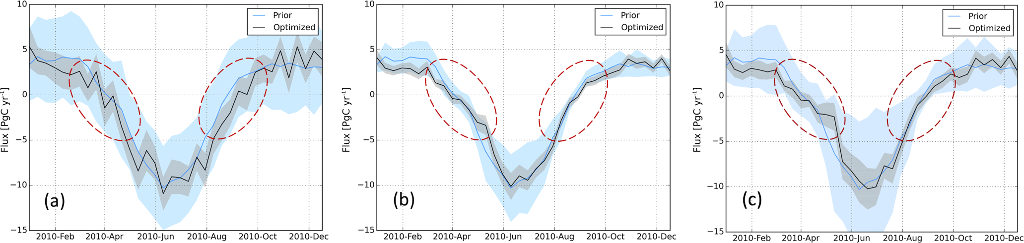
Figure 8 Comparison between two flux optimization methods: the additive method (a) gives significant different optimized fluxes, highlighted by the red dashed ellipses, in contrast to the multiplicative method (b), and (c) is similar to (b) but with 2 times the flux uncertainty, i.e., setting the biosphere scaling parameter variance to 160 %. The additive method seems more flexible to adjust fluxes in case net carbon exchange is small or even close to zero around the shoulder seasons (spring/fall).

The prior/optimized fluxes using both additive and multiplicative flux adjustment methods are shown in Fig. 8. We found that major differences occur in the so-called shoulder seasons, where the flux adjustment is significant for the run with the additive method but is negligible for the run with the multiplicative method. The multiplicative method fails to adjust the fluxes in this case because the NEE is small or even close to zero around the shoulder seasons. Larger variations in the optimized fluxes for the additive flux adjustment method are observed compared to those for the multiplicative method, due to the flexibility of the additive flux adjustment method and higher prior flux uncertainties. Note that both methods reproduce observed CO₂ values equally well and multiplicative scalars do not lead to worse residuals.

Figure 9 shows the inversion results of model runs with pseudo-data, further confirming the advantage of the additive method over the multiplicative method in the CTDAS-Lagrange system. The additive method recovers the seasonality better than the multiplicative method, noticeable mainly for the period June–July. It is also clearly shown that the multiplicative method fails to derive the “truth” fluxes around the shoulder season in the fall (no difference between the prior and the truth in the spring). Besides this, the estimate of the annual net biosphere fluxes derived from the additive method is also closer to the truth than that from the multiplicative method, although the associated uncertainties are rather large.

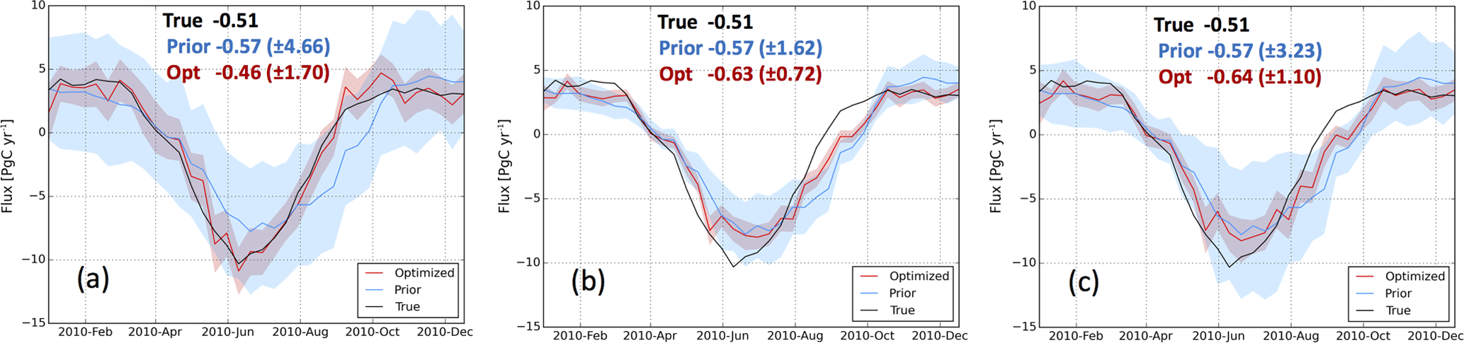
Figure 9 Comparison of the performance of inversions with pseudo-data using the two flux optimization methods: (a) the additive method and (b) the multiplicative method, (c) is similar to (b) but with 2 times the flux uncertainty, i.e., setting the biosphere scaling parameter variance to 160 %. The “truth” fluxes are generated in a forward simulation using biosphere fluxes from SiBCASA. The same SiB3 fluxes are used as a priori for all runs. The annual net biosphere fluxes of the truth, prior, and optimized are given in the legend, with the unit of PgC yr⁻¹.

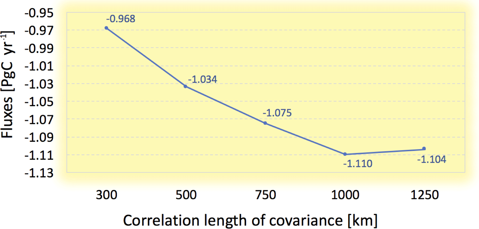
Figure 10 Sensitivity of the optimized annual net biosphere fluxes (PgC yr⁻¹) as a function of the chosen covariance length scale (km). The optimized fluxes tend to converge to −1.1 PgC yr⁻¹ when the length scale is larger than 750 km.

3.6 Sensitivity to the covariance length scale

The sensitivity of the CTDAS-Lagrange to the covariance length scale is shown in Fig. 10. The optimized fluxes tend to reach a robust value when the covariance length scale is larger than 750–1000 km, and we note that the difference between 750 and 1000 km is relatively small. We have tested whether including aircraft sites can reduce this length scale dependence below 1000 km, and find it can slightly alleviate the dependence but does not fully resolve that. The optimized fluxes for the temperate North America are relatively insensitive to the covariance length scale, as this region is relatively well sampled by the dataset. We have only used some of the available observations, and different results may be found when additional data are included, e.g., from Environment Canada tower sites.

3.7 Ensemble estimates

From the above-described sensitivity runs, we derive an ensemble of estimates of optimized North American annual net biosphere fluxes in 2010 (see Fig. 11). The optimized biosphere fluxes of all the runs are larger (i.e., more uptake) than their corresponding prior fluxes. Compared to other factors, the prior biosphere fluxes have the largest impact on the optimization result. The selection of model–data mismatch with 3 ppm is reasonable, judging from the observed small differences between the model runs BASE and R2 (4 ppm). We notice the R1 (2 ppm) run makes a significant difference, as it rejects much more observations than the other two cases, especially during summertime when usually larger mismatches between observations and simulations occurred (not shown).

Comparing BASE, Q1 (decrease the magnitude of additive uncertainty by 50 %), and Q2 (increase the magnitude of additive uncertainty by 50 %), we find the prior uncertainty magnitude ascribed to biosphere fluxes impacts the result only a little, with small reductions in the optimized flux when the uncertainty gets larger. In addition, we find that our system is sensitive to the uncertainty in the BC parameter Pbc1 (1 ppm uncertainty) and Pbc2 (3 ppm uncertainty), which results in the difference of flux estimates by slightly more than 0.1 PgC yr⁻¹. The choice of 2 ppm is according to the uncertainties we assessed from the statistics between these different prior BCs we used. When the two tower sites STR and WGC that are located close to the west coast of North America are excluded, we find smaller biosphere fluxes (the difference is approximately 0.15 PgC yr⁻¹), which indicates that attention should be paid to the choice of the observations.

Excluding results from B2 that we consider unrealistic due to the high data rejection rate (replaced by the B2^′ run), we estimate North American carbon fluxes for the year 2010 to be between −0.92 and −1.26 PgC yr⁻¹.

4 Conclusions and discussion

We have implemented a regional carbon assimilation system based on the CarbonTracker Data Assimilation Shell framework and a high-resolution Lagrangian transport model WRF-STILT. The new system, named CTDAS-Lagrange, optimizes both biosphere fluxes and four boundary condition (BC) parameters and is computationally efficient (1 year of optimization can be performed serially within 14 h with eight threads on a 12-core Intel Xeon processor E5 v2 family computer with a processor base frequency of 2.7 GHz, once footprints are calculated and stored offline). Furthermore, we have demonstrated that the additive flux adjustment method is more flexible in optimizing NEE than the multiplicative flux adjustment method, especially in the shoulder seasons of the year.

The sensitivity test results with three different lateral BCs (CT2013B, CTE2014, and an empirical curtain) indicate that CTDAS-Lagrange has the ability to largely correct for the potential biases in the lateral BCs, with the BC optimization absorbing up to 0.23 PgC yr⁻¹ of flux adjustment that would otherwise have been made to the optimized annual net biosphere fluxes. This makes the CTDAS-Lagrange system less dependent on the choice of lateral BCs than a system without BC optimization or offline correction. The sensitivity tests with two alternative biosphere fluxes (SiB3 and CT2013B-avg) and a series of modified SiBCASA fluxes with a large range of NEE show that the seasonal magnitude of the optimized fluxes is almost independent of the prior fluxes, and the optimized annual net biosphere fluxes converge for SiB3 and CT2013B-avg and are much less dependent on the range of the priors for the series of modified SiBCASA fluxes. This demonstrates that the CTDAS-Lagrange system is capable of resolving large biases in the prior biosphere fluxes. On the other hand, the optimized annual net biosphere fluxes with different prior fluxes are less convergent at the ecoregion level, presumably due to the limited choice of observational constraints. This could also be improved by better prescribing the uncertainties in biosphere fluxes for the additive adjustment method, as the assumption of spatially and temporally uniform flux uncertainties may not be reasonable.

We derive an ensemble of estimates of the optimized annual net biosphere carbon fluxes based on a series of sensitivity tests, which places the North American Carbon sink for the year 2010 at −0.92 to −1.26 PgC yr⁻¹, comparable to the TM5-based estimates of CarbonTracker (version CT2016, $-\mathrm{0.91}\pm \mathrm{1.10}$ PgC yr⁻¹, data obtained from https://www.esrl.noaa.gov/gmd/ccgg/carbontracker/, last access: 25 August 2018) and CarbonTracker Europe (version CTE2016, $-\mathrm{0.91}\pm \mathrm{0.31}$ PgC yr⁻¹; van der Laan-Luijkx et al., 2017). Note that much less observations have been used in CTDAS-Lagrange than those assimilated in CT2016 and CTE2016. This work is to be followed up by a multi-year inversion using more available observations in recent years, and by assimilating an additional tracer, carbonyl sulfide, to simultaneously constrain both GPP and NEE.

In addition, the estimate of net CO₂ uptake for the year 2010 is reasonable compared to an ensemble of atmospheric inversions from several studies that place the North American NEE for 2000–2006 at $-\mathrm{0.931}\pm \mathrm{0.670}$ PgC yr⁻¹ (Hayes et al., 2012), and a more recent study suggesting the North American net CO₂ biosphere fluxes during 2000–2009 to be $-\mathrm{0.890}\pm \mathrm{0.400}$ PgC yr⁻¹ from the RECCAP-selected TransCom3 inversions (King et al., 2015). Three atmospheric inversion studies placed North American NEE for the year 2004, which had been recognized as a climate-favorable year for uptake, from $-\mathrm{0.953}\pm \mathrm{0.106}$ to $-\mathrm{1.230}\pm \mathrm{1.120}$ PgC yr⁻¹ (CT2011, Peters et al., 2007; Butler et al., 2010; Gourdji et al., 2012). However, we also note that although we have a comparable estimate to the two versions of CarbonTracker at the continental scale, our estimates at ecoregion scales are different. Typically the boreal region is not well constrained in our study with eight tower sites located in the US, while no data from the extensive network of Environment Canada was used. To solve finer-scale fluxes, the use of data from a denser observational network is desirable and could likely further reduce the chosen covariance length scale shown in Fig. 10.

Although we have accounted for the impact of possible biases in the prior lateral BCs on optimized fluxes, we find that there remains room to further reduce the biases at surface sites (shown in Table 1 as posterior residuals). This could be partially because aircraft observations are sparse, and are temporally insufficient for sampling the inflows of the continent. Also, the limited number of parameters used for BC adjustments could be a bottleneck; an alternative scheme with more extensive parameterization to offer more flexibility for BC adjustments could help.

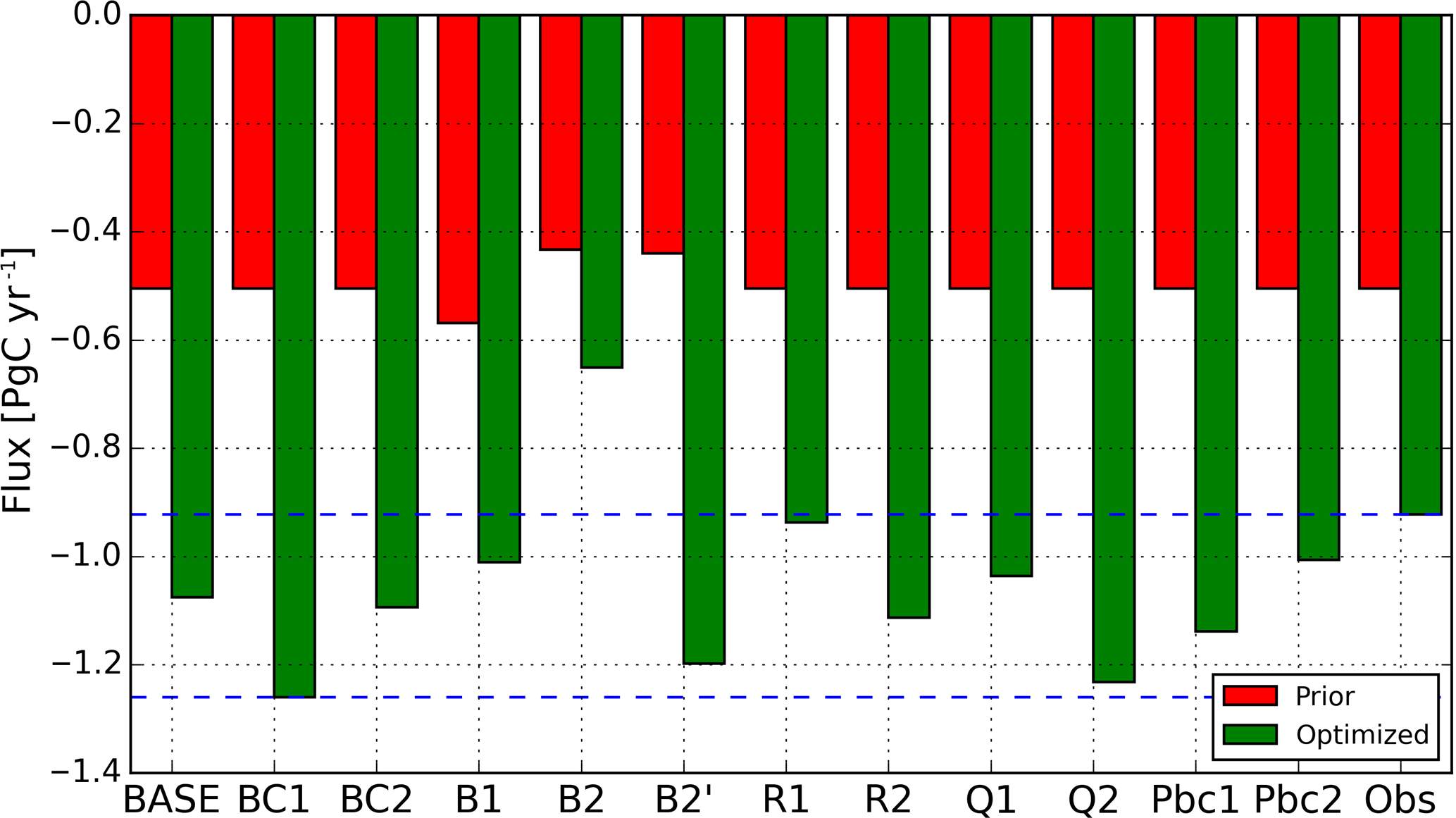
Figure 11 North American 2010 annual net biosphere fluxes (PgC yr⁻¹) estimated from an ensemble of CTDAS-Lagrange runs with different prior biosphere fluxes, different CO₂ BCs, and model setup choices. The dashed blue lines refer to the range of the ensemble estimates −0.92 to −1.26 PgC yr⁻¹ excluding the B2 run. See Table 2 for an overview of all experiments.

Moreover, the optimization results of the CTDAS-Lagrange system depend on the quality of the forward simulations, i.e., fixed a priori fluxes and transport models. The optimization of biosphere fluxes may be influenced by observations affected by local fossil fuel signals, which can be addressed by using high-resolution fossil fuel emissions or filtering out the observations. CO has long been studied and used as a tracer for fossil fuel emissions, and its use as a quantitative tracer suffers mainly from varying emission ratios of different sources and production by oxidation of hydrocarbons. We have used CO as a fossil fuel tracer to filter out observations that are considerably affected by fossil fuel emissions, which is expected to serve our purpose reasonably well in wintertime; however, this may not be appropriate on the occasions when production of CO by oxidation of hydrocarbons can be significant in summertime. Thus the CO filtering may have been overly conservative, reducing the number of observations by up to ∼7 % (the average percentage at all sites) in summertime. As we use the same filtered dataset for all the model runs, and the CTDAS-Lagrange system rejects observations when the difference between simulated and observed CO₂ is larger than 3 times the assigned model–data mismatch, the potential issue of inappropriate CO filtering in summertime is unlikely to significantly bias our results. Efforts have been made to assimilate both CO₂ and ¹⁴CO₂, a tracer for recently added fossil fuel, to optimize both biosphere and fossil fuel fluxes (Basu et al., 2016; Fischer et al., 2017). To investigate the influence of the transport model, we have performed tests with an alternative Lagrangian transport model, the Hybrid Single Particle Lagrangian Integrated Trajectory (HYSPLIT; Draxler and Hess, 1998; Stein et al., 2015) model driven by the North American Mesoscale Forecast System meteorological fields at 12 km resolution (NAM12). Our preliminary results show that the HYSPLIT-NAM12 run yields similar biosphere uptake in summertime, but higher respiration fluxes in wintertime. Hegarty et al. (2013) showed that the three widely used Lagrange particle dispersion models (LPDMs), HYSPLIT, STILT, and FLEXible PARTicle (FLEXPART; Stohl et al., 2005) have comparable skills in simulating the plumes from controlled tracer release experiments when driven with identical meteorological inputs. Thus, the observed difference is most likely caused by the difference between WRF and NAM12. A second reason could be attributed to the fact that the WRF domain is larger and extends much further to the north than the NAM12 files archived by NOAA Air Resources Laboratory (https://ready.arl.noaa.gov/hypub/ hysp_meteoinfo.html, last access: 25 August 2018). Therefore, compared to the NAM12 run, the WRF-STILT run covers a larger area, and is less influenced by the potential biases in the northern boundary that is nontrivial to correct due to the large latitudinal gradients in CO₂ mole fractions. A further detailed investigation into the differences between the two meteorological inputs is required to diagnose the resulting difference in the optimized fluxes in wintertime; however, this task is beyond the scope of the development of our CTDAS-Lagrange system.

We highlight that the use of aircraft data in this study suggests a very important constraint from free tropospheric measurements to the lateral BCs, which enables simultaneous optimization of BCs and biosphere fluxes. Our system is an open framework for regional atmospheric inversions that could be extended to use different atmospheric transport models, to study other trace gases, and for alternative geographic regions.