Closing the energy balance using a canopy heat capacity and storage concept – a physically based approach for the land component JSBACHv3.11

Land surface–atmosphere interaction is one of the most important characteristic for understanding the terrestrial climate system, as it determines the exchange fluxes of energy and water between the land and the overlying air mass.

In several current climate models, it is common practice to use an unphysical approach to close the surface energy balance within the uppermost soil layer with finite thickness and heat capacity. In this study, a different approach is investigated by means of a physically based estimation of the canopy heat storage (SkIn⁺).

Therefore, as a first step, results of an offline simulation of the land component JSBACH of the Max Planck Institute Earth system model (MPI-ESM) – constrained with atmospheric observations – are compared to energy fluxes and water fluxes derived from eddy covariance measurements observed at the CASES-99 field experiment in Kansas, where shallow vegetation prevails. This comparison of energy and evapotranspiration fluxes with observations at the site-level provides an assessment of the model's capacity to correctly reproduce the diurnal cycle. Following this, a global coupled land–atmosphere experiment is performed using an AMIP (Atmospheric Model Intercomparison Project) type simulation over 30 years to evaluate the regional impact of the SkIn⁺ scheme on a longer timescale, in particular, with respect to the effect of the canopy heat storage.

The results of the offline experiment show that SkIn⁺ leads to a warming during the day and to a cooling at night relative to the old reference scheme, thereby improving the performance in the representation of the modeled surface fluxes on diurnal timescales. In particular: nocturnal heat releases unrealistically destroying the stable boundary layer disappear and phase errors are removed. On the global scale, for regions with no or low vegetation and a pronounced diurnal cycle, the nocturnal cooling prevails due to the fact that stable conditions at night maintain the delayed response in temperature, whereas the daytime turbulent exchange amplifies it. For the tropics and boreal forests as well as high latitudes, the scheme tends to warm the system.

1 Introduction

The land surface plays a key role in climate modeling because it regulates a number of biogeophysical as well as biogeochemical processes (Sellers et al., 1997). The former process controls the partitioning of available energy – depending on the surface albedo – into ground and into turbulent heat fluxes. This results in surface temperature changes that effect the diurnal variation of the boundary layer development and govern convection and cloud formation. This energy cycle is coupled with the water cycle dividing the available precipitated water into runoff, drainage, and infiltration leading to soil moisture changes which influence the evapotranspiration. In contrast, the biogeochemical processes are mainly represented by the terrestrial carbon sink which is strongly coupled to the water cycle through the leaves' stomatal control of photosynthesis and transpiration.

In the past, land–atmosphere interactions were associated with low vertical scale phenomena limited to the atmospheric boundary layer without an impact on larger scales or on the climate system. However, over the last few decades, many studies and research papers have proven this assumption to be false (Pitman, 2003). The development of land surface models (LSM), used in numerical weather prediction and in climate models, started by using the so-called “bucket scheme” which was based on the theory that the soil was composed of boxes which could store limited amounts of water (Manabe, 1969). A few years later, Blackadar (1976) developed a two-layer model with a thin variable surface layer influenced by changeable radiation and a thick sluggish deeper layer that changed its temperature governed by a wave equation. A subsequent pioneering study in the design of LSMs was the introduction of a multilayer soil model by Deardorff (1978) who included a new method for predicting soil moisture content.

These improvements became especially relevant on the global scale when land–atmosphere transfer schemes (including a biosphere) were included in general circulation models (GCM). These models were concurrently investigated by Dickinson et al. (1986) and Sellers et al. (1986), who demonstrated the need to evaluate current LSM developments using observation-based data. The first systematic effort in this direction was PILPS (the Project for the Intercomparison of Land-Surface Parameterization Schemes) (Henderson-Sellers et al., 1993). Here, synthetic atmospheric forcing data were used to improve the parameterization of the continental surface. The first results of experiments forced with real atmospheric boundary layer data were documented by the widely quoted work of Chen et al. (1997) comparing 23 different land surface schemes.

Two years later, the conclusions drawn by the point-based PILPS experiments were extended to global scales in the Global Soil Wetness Project (GSWP) (Dirmeyer et al., 1999) which required a processed atmospheric forcing data set. Only a year later, a new project was founded that followed the idea of combining PILPS with its local-scale character and GSWP which is based on a global perspective; this ongoing joint project is called the Global Land Atmosphere System Study (GLASS). In the last decade and a half, GLASS has broadly expanded and various other projects have joined. The main goal of this effort is to improve land surface schemes for the benefit of numerical weather prediction and climate models.

Over the last few years, JSBACH, the model used in this study, has been used for a considerable number of different applications, including being utilized in a coupled global context on long timescales to study various biogeochemical and biogeophysical aspects such as the carbon cycle (Claussen et al., 2013; Raddatz et al., 2007), natural and anthropogenic land cover change (Pongratz et al., 2008; Reick et al., 2013), vegetation cover and land surface albedo (Brovkin et al., 2013), and atmosphere–forest interaction and feedbacks (Brovkin et al., 2009; Otto et al., 2011). In addition to these aspects, the physical components, which regulate the exchange of energy and water fluxes, have been studied (Hagemann and Stacke, 2015; Knauer et al., 2015; de Vrese and Hagemann, 2016). However, the performance of JSBACH on shorter timescales such as the diurnal cycle has not yet been tested. An exception to this is the study by Schulz et al. (2001) who modified the numerical time integration scheme from a semi-implicit scheme, which does not conserve energy, to an energy conserving implicit land–atmosphere coupling scheme. This scheme has been evaluated in so-called “offline” experiments using data from the Cabauw (Netherland) tower on diurnal timescales.

Despite this vast development and progress in modeling land surface processes, it is still common practice for several current climate models – JSBACH included – to use a prognostic procedure to close the surface energy balance within a soil layer of a finite heat capacity. In this study, a different approach is investigated. Following Viterbo and Beljaars (1995) we close the energy balance diagnostically (i.e., neglecting the time derivative) at an infinitesimally thin layer that is located at the surface of the vegetated land. Conveniently, the new scheme is abbreviated by “SkIn” which stands for “Surface is Kept INfinitesimally thin”, in addition to the fact that this scheme represents a layer with a negligible vertical extent comparable with a thin “skin”.

To test the performance of the scheme, we initially carried out an offline single site experiment with the land component JSBACH of the MPI-ESM (for more information see Sect. 2.1). In an offline experiment the LSM is decoupled from its host model and forced by observation data; it is then evaluated against observed fluxes. Therefore, initial data, forcing data, and verification data from the Diurnal Land–Atmosphere Coupling Experiment (DICE) (Zheng et al., 2013) (for more information see Sect.2.3) were used to compare energy fluxes and water fluxes derived from eddy covariance measurements observed at the CASES-99 field experiment in Kansas with simulated fluxes. This first experiment was designed to establish if the SkIn scheme would improve the performance of reproducing the diurnal cycle in comparison to the old heat storage concept in cases with shallow vegetation.

Following this, a global coupled land–atmosphere model experiment with the MPI-ESM was performed using the so-called AMIP (Atmospheric Model Intercomparison Project) protocol (Gates, 1992). In this experiment the MPI-ESM (with T63 resolution, i.e., 1.9^∘) was run covering 30 years from 1979 to 2008 with prescribed sea surface temperatures. For this global experiment an extended approach was applied. Following Moore and Fisch (1986), we took the energy storage in the canopy layer into account by replacing the unphysical heat storage approach in the energy balance equation with a physically based estimation of the heat storage of the canopy air space and of the biomass itself.

The importance of the so-called “canopy heat storage” in connection with the solution of the energy balance equation has been estimated in several experimental studies at the site-level (Jacobs et al., 2008). Meyers and Hollinger (2004) showed that the combined energy of all of the different types of canopy heat storages (e.g., the energy flux for photosynthesis as well as the canopy heat storage in biomass and water content) can amount to 15 % of the net radiation even for crop sites. However, the simulated estimation of the canopy heat storage for longer timescales on global scale remained disregarded. Thus, the second experiment was designed to establish if the extended SkIn scheme (SkIn⁺) would show a regional impact on longer timescales, and if so, to establish if the current biases in near surface temperature were at least partly caused by the former oversimplified parameterization of the surface energy balance.

First, the physics of the climate model used for this study and its modifications regarding both above mentioned new approaches are depicted, followed by a description of the data used for the single site experiment (Sect. 2). Next, the results of both experiments are interpreted (Sect. 3) and the most important outcomes are discussed (Sect. 4) and summarized (Sect. 5).

2 Model, data, and experiments

In this section, the differences between the standard model and the modified model are analyzed. Following this, the data and the site for the offline experiment are described and the designs of both evaluation experiments are explained.

2.1 Model description

JSBACH (version 3.11) is the land component of the MPI-ESM (the Max Planck Institute Earth system model, version 6.3.03). In the past, it was embedded in ECHAM (EC following ECMWF and HAM representing Hamburg), the atmospheric component of MPI-ESM (Stevens et al., 2013). Since 2005, JSBACH is a full representation of the global soil–vegetation–atmosphere transfer system (Raddatz et al., 2007) that can also be run independently as a so-called “offline” version forced by climate data. The physical core components of the land processes (energy balance, heat transport, and water budget) are adopted from ECHAM5 (Roeckner et al., 2003) with a fully implicit land-surface–atmosphere coupling scheme (Schulz et al., 2001). This means that the mutual boundary conditions between the land surface and the atmosphere, in the form of air temperature and specific humidity at the lowest atmospheric level, are formulated as implicit functions of the surface conditions at the new time step. The surface radiation follows a scheme which allows albedo changes of the surface below the canopy (Vamborg et al., 2011), and the soil hydrology is calculated using a five-layer scheme (Hagemann and Stacke, 2015). To represent the dynamics of land carbon uptake and release, JSBACH contains the photosynthesis and canopy radiation components from the BETHY (Biosphere Energy-Transfer Hydrology) model (Knorr, 2000), a prognostic phenology scheme, and components for uptake, storage, and release of carbon from vegetation and soils (Brovkin et al., 2009). Natural land cover changes are simulated prognostically by a dynamic vegetation module which includes the representation of the subgrid-scale heterogeneity of vegetation classes (Reick et al., 2013). Anthropogenic land use and land cover changes are prescribed either by maps or by forcing data from the New Hampshire Harmonized Protocol (Hurtt et al., 2011).

To simulate land surface and soil processes in JSBACH, the energy and water exchange within the soil is described by the diffusion equations for heat and moisture on a multi-layer vertical grid extending to a depth of 10 m. The soil is divided into five layers (Hagemann and Stacke, 2015) that grow in thickness with increasing soil depth. The diffusion equation for heat

$$\begin{array}{}\text{(1)}& {\displaystyle }(\mathit{\rho }C{)}_{\mathrm{soil}}{\displaystyle \frac{\partial T_{\mathrm{soil}}}{\partial t}}={\displaystyle \frac{\partial }{\partial z}}\left({\mathit{\lambda }}_{\mathrm{soil}}{\displaystyle \frac{\partial T_{\mathrm{soil}}}{\partial z}}\right)\end{array}$$

is solved numerically following the method from Richtmyer and Morton (1967). In Eq. (1) (ρC)_soil denotes the volumetric soil heat capacity [J (m³K)⁻¹], λ_soil is the soil thermal conductivity [W (m K)⁻¹], and T_soil is the soil temperature. A zero flux boundary condition for heat is applied at the bottom of the soil, and at the top of the soil the temperature of the uppermost soil layer is considered as the surface temperature. Therefore, this implies that the ground heat flux is the heat exchange between the first and the second soil layers. An analogous equation, which governs the vertical diffusion for moisture, is represented by the one-dimensional Richards equation (that is described in detail by Hagemann and Stacke (2015)). To couple JSBACH and the atmosphere, the surface energy balance and surface water balance are solved to provide the boundary conditions for the two abovementioned diffusion equations; this represents a link between the atmosphere and the underlying soil. The water balance at the surface describes the changes in surface water caused by precipitation, evapotranspiration, snow melt, surface runoff, and infiltration. Additionally, the snow budget and the interception reservoir of rain and snow is determined to close the entire water balance; a detailed description of these processes can be found in the ECHAM5 documentation (Roeckner et al., 2003).

The surface energy balance is calculated by partitioning the available net radiation (R_net) into the ground heat flux (G), the turbulent sensible heat flux (H), and the latent heat flux (LE), where the latter two represent a forcing for the atmospheric component in the coupled system. In JSBACH the energy balance is closed, i.e., calculated and evaluated, within the uppermost soil layer including a heat storage term $S_{\mathrm{soil}}=C_{\mathrm{soil}}\partial T_{\mathrm{sfc}}/\partial t$ corresponding to the term on the left hand side that is proportional to the time derivative of the surface temperature:

$$\begin{array}{}\text{(2)}& {\displaystyle }{C}_{\mathrm{soil}}{\displaystyle \frac{\partial T_{\mathrm{sfc}}}{\partial t}}=R_{\mathrm{net}}+H+\text{LE}+G.\end{array}$$

Here, C_soil corresponds to the area-specific heat capacity of the uppermost soil layer [J (m²K)⁻¹]. The surface fluxes of heat, water, and momentum are defined using the bulk formulation based on the surface-layer similarity theory. These can be expressed by the so-called “atmospheric resistance”, which is the inverse product of the wind speed and the drag coefficient. The latter represents a measure of the turbulence strength determined by the roughness of the underlying surface and the influence of atmospheric stratification, which is quantified by empirical stability functions derived by Louis (1982, 1979) that depend on the Richardson number. The roughness lengths as well as the drag coefficients are assumed to be different for momentum and scalar quantities (Brutsaert, 1975). Over vegetated surface, the turbulent fluxes of heat, water, and momentum are also given by the resistance law. However, an additional canopy resistance is added in the calculation of the water vapor fluxes. It depends on the photosynthetically active radiation and on the leaf area index. In addition, it is modified by a water stress factor depending on the soil water within the root zone. All these parameterizations include variables which, in turn, are functions of the surface temperature. Moreover, the surface temperature appears to the forth power in the description of the outgoing longwave part of the net radiation. Also the formulation of the latent heat flux exhibits a nonlinear temperature dependence. According to these dependencies, the energy balance equation (Eq. 2) and its alterations (Eqs. 3 and 4 in the following) represent complex implicit nonlinear equations.

2.2 Model modifications

In the standard scheme of JSBACH the surface energy balance is closed within the uppermost soil layer of finite thickness (6.5 cm) and heat capacity. However, as the absorption of radiation takes place in the uppermost micrometers of the soil, this assumption appears unrealistic. Therefore, in the SkIn approach a surface temperature T_sfc that corresponds to an infinitesimally thin interface between the soil, the vegetation, and the atmosphere is calculated. Hence, in this case the prognostic energy balance (Eq. 2), which contains a heat storage term, is changed to a diagnostic energy balance equation where the surface energy balance is closed for an infinitesimally thin surface:

$$\begin{array}{}\text{(3)}& {\displaystyle }{R}_{\mathrm{net}}+H+\text{LE}+G=\mathrm{0}.\end{array}$$

We note that the use of the instantaneous response temperature is not a novel approach. This so-called “skin temperature” was introduced by Viterbo and Beljaars (1995) to replace the old ground-surface model of the ECMWF. This approach is also used in other land surface models, e.g., in the community Noah land surface model (Niu et al., 2011). To solve the diagnostic energy balance (Eq. 3) explicitly, the nonlinear terms – which are related to the outgoing longwave radiation described by the Stefan–Boltzmann law as well as to the temperature-dependent specific saturated humidity of the surface – have to be linearized. Here, a first-order Taylor approximation was chosen. Neglecting the heat storage term results in a loss of stability in the numerical solution because the storage term exerts a dampening effect. Therefore, the surface instantly reacts to variations in the forcing data, especially to intense fluctuations in solar radiation flux densities or to wind speed variations. As a consequence, the first guess of the solution using the linearizations is insufficient and an iteration is needed to stabilize the system. For this implementation a simple Newton iteration combined with a fixed-point iteration was used where the surface temperature of the previous time step is used as a first guess starting point. Further tests have shown that it is not sufficient to only update the outgoing longwave radiation as a part of the net radiation and the saturated specific humidity every iteration step. In addition, the drag coefficient of heat must be included in the iteration loop as well, as it nonlinearly depends on the surface temperature. Taking the drag coefficient of heat into account in the iterative procedure exerts a negative feedback ensuring the stability of the numerical solution of the energy balance equation.

In addition, the implicit numerical scheme for the heat diffusion equation of the soil layer, which is based on the Richtmyer and Morton scheme (Richtmyer and Morton, 1967), has to be adjusted. This is due to the fact that the ground heat flux no longer describes a conductive heat transfer between the two uppermost soil layers but instead depends on the heat exchange between the uppermost soil or snow layer and the overlying canopy air mass. Therefore, the ground heat flux $G={\mathrm{\Lambda }}_{\mathrm{sfc}}\left(T_{\mathrm{1}}-T_{\mathrm{sfc}}\right)$ is assumed to be proportional to the temperature difference between the surface and the uppermost soil layer T₁. The constant of proportionality constitutes an empirically determined factor, the so-called “heat transfer coefficient” Λ_sfc [W (m²K)⁻¹], which was introduced by Viterbo and Beljaars (1995) (they used the notation skin conductivity). Different values are assigned – predominantly between 10 and 40 W (m²K)⁻¹ – for the heat transfer coefficient depending on the plant functional type (PFT). The values used for Λ_sfc in the present study can be found in Trigo et al. (2015).

The concept of the surface temperature characterizing an infinitesimally thin surface, in which the heat storage is completely neglected, is only valid for areas where bare soil or shallow vegetation prevails; it is considered as a special case which is analyzed in an offline single site experiment located in Kansas' grassy landscape (for a detailed description see Sect. 2.3). For the global evaluation experiment, which includes forest regions such as the tropical rain forest (that has a dense canopy of up to 45 m high) this approach is insufficient. In this case, the change in total heat content (in short heat storage) of the canopy air, the water vapor, and the biomass itself is no longer negligible. Therefore, the canopy heat storage (S_cano), which is based on a formulation given by Moore and Fisch (1986), is introduced into the energy balance equation:

$$\begin{array}{}\text{(4)}& {\displaystyle }{S}_{\mathrm{cano}}=\mathrm{LE}+H+G+R_{\mathrm{net}}.\end{array}$$

It is composed of the sum of three parts

$$\begin{array}{}\text{(5)}& {\displaystyle }{S}_{\mathrm{cano}}=S_T+S_{\mathrm{veg}}+S_q,\end{array}$$

where S_T denotes the heat storage in the canopy air space, S_veg represents the heat storage of biomass, and S_q represents the heat storage resulting from changes in specific humidity in the canopy layer (in short, the latent heat storage). The heat storage in the canopy air space S_T can be expressed as

$$\begin{array}{}\text{(6)}& {\displaystyle }{S}_T=C_T{\displaystyle \frac{\partial T_{\mathrm{sfc}}}{\partial t}}=c_p{\mathit{\rho }}_{\mathrm{a}}{z}_{\mathrm{veg}}{\displaystyle \frac{\partial T_{\mathrm{sfc}}}{\partial t}},\end{array}$$

where C_T is the area-specific heat capacity of the canopy air, c_p=1005 J (kg K)⁻¹ is the specific heat capacity of air at constant pressure, ρ_a is the density of air, and z_veg is the vegetation height. The heat storage of biomass in the canopy layer (S_veg) is determined as

$$\begin{array}{}\text{(7)}& {\displaystyle }{S}_{\mathrm{veg}}=C_{\mathrm{veg}}{\displaystyle \frac{\partial T_{\mathrm{sfc}}}{\partial t}}=c_{\mathrm{veg}}{m}_{\mathrm{veg}}{\displaystyle \frac{\partial T_{\mathrm{sfc}}}{\partial t}},\end{array}$$

where C_veg is the area-specific heat capacity of the biomass, m_veg is the area specific mass of biomass, and c_veg is the specific heat capacity of moist biomass according to Moore and Fisch (1986). The latter is approximated by a weighted average between the specific heat capacity of dry biomass containing a temperature dependence and the specific heat capacity of water c_w=4184 J (kg K)⁻¹ assuming a constant water mixing ratio. For example, at a temperature of 25 ^∘C the canopy biomass has a specific heat capacity of c_veg≈2650 J (kg K)⁻¹. The area specific mass of moist biomass (m_veg) can be estimated as a function of the vegetation height (z_veg) using a linear relationship, namely m_veg=ρ_vegz_veg, where ρ_veg≈1.67 kg m⁻³ is the partial density of moist biomass, i.e., the mass of moist biomass per one cubic meter of air estimated using values given by Moore and Fisch (1986).

The latent heat storage (S_q) can be calculated according to Moore and Fisch (1986) as follows:

$$\begin{array}{}\text{(8)}& {\displaystyle }{S}_q=L_{\mathrm{v}}{\mathit{\rho }}_{\mathrm{a}}{z}_{\mathrm{veg}}{\displaystyle \frac{\partial q_{\mathrm{cas}}}{\partial t}},\end{array}$$

where $L_{\mathrm{v}}=\mathrm{2.5}\times {\mathrm{10}}^{\mathrm{6}}$ J kg⁻¹ denotes the latent heat of vaporization and q_cas represents the specific humidity in the canopy air space. In contrast to the heat storages of the canopy air and the biomass – Eqs. (6) and (7) – which are expressed by means of heat capacities related to the time derivative of surface temperature, the situation is more complicated regarding the latent heat storage: changes in specific humidity can occur independently of temperature changes. This means, that only considering changes in specific humidity due to changes in surface temperature would neglect other humidity sources and sinks. Thus, a different approach to parameterize the latent heat storage is required because the current schemes does not contain a prognostic variable for the specific humidity in the canopy air space. In this approach, we take the heat storage resulting from changes in specific humidity of the canopy air space into account by defining an effective surface specific humidity (q_sfc), which is the best proxy for the specific humidity in the canopy layer that we have. It represents a nonlinear weighted average between the specific air humidity above the canopy (q_air) and the saturated specific humidity at the surface temperature, q_sat(T_sfc), by demanding that

$$\begin{array}{}\text{(9)}& {\displaystyle \frac{q_{\mathrm{air}}-q_{\mathrm{sfc}}}{r_{\mathrm{a}}}}\stackrel{!}{=}\text{LE}\left(q_{\mathrm{air}},q_{\mathrm{sat}}\left(T_{\mathrm{sfc}}\right),r_{\mathrm{a}},r_{\mathrm{c}},\mathrm{\dots }\right),\end{array}$$

where r_a is the atmospheric resistance, r_c is the canopy resistance, and LE is the latent heat flux as it is calculated in the energy balance equation. This means that q_sfc is calculated to represent the effective near surface specific humidity that is required to reproduce the surface moisture fluxes due to turbulent exchange processes. In principle, the specific humidity of the boundary layer, q_air, could be used as a proxy for the canopy air space humidity, q_cas, as suggested by Moore and Fisch (1986). However, we are of the opinion that the usage of q_air would underestimate the latent heat storage in the current scheme. This leads to a modified formulation of the latent heat storage, S_q:

$$\begin{array}{}\text{(10)}& {\displaystyle }{S}_q=L_{\mathrm{v}}{\mathit{\rho }}_{\mathrm{a}}{z}_{\mathrm{veg}}{\displaystyle \frac{\partial q_{\mathrm{sfc}}}{\partial t}}.\end{array}$$

Because q_sfc is not a prognostic variable in the energy balance, its time derivative is approximated using values of q_sfc at previous time steps. This is an approximation that is inevitable in the current model framework and can only be avoided by developing an extended dual source canopy layer scheme which includes a prognostic specific humidity of the canopy air space as mentioned in the discussion (see Sect. 4). Using these approaches, the former unphysical soil heat storage concept in the surface energy balance equation was replaced by a physically based estimation of the canopy heat storage.

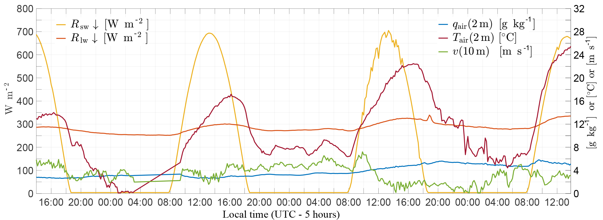
Figure 1 DICE forcing data used for the offline single site experiment in the form of longwave downward radiation (R_lw ↓, orange) and shortwave downward radiation (R_sw ↓, yellow) in W m⁻² (see left axis), as well as the 10 m wind speed (v, m s⁻¹, green), the 2 m air temperature (T_air, ^∘C, red), and the 2 m specific humidity (q_air, g kg⁻¹, blue) (see right axis). Data are from the CASES-99 experiment in Kansas from 23 to 26 October 1999.

When discussing heat storages within the canopy one also has to consider the energy stored in the form of chemical energy by carbohydrate bonds through the process of photosynthesis. Following Nobel (2009) the energy required to incorporate 1 mol CO₂ is 479 kJ. That means, a CO₂ flux of 1 mg CO₂ (m²s)⁻¹ corresponds to an energy flux of about 11 W m⁻². This chemical heat storage has been evaluated in several experimental studies at the site-level (Jacobs et al., 2008; Meyers and Hollinger, 2004). However, in these studies emphasis has only been on the energy consumption through photosynthesis (GPP, i.e., gross primary production). The fact that heat will also be released during the process of plant respiration (Thornley, 1971; Wohl and James, 1942) has been neglected in most studies. This had led to an overestimation of the chemical heat storage. Thus, one has to consider not only the net primary production (NPP) but also all other processes that release CO₂. Therefore, we added an additional term in the energy balance to estimate the magnitude of the heat stored in chemical bonds:

$$\begin{array}{}\text{(11)}& {\displaystyle }{S}_{\mathrm{cano}}=\mathrm{LE}+H+G+R_{\mathrm{net}}+\mathit{\beta }{F}_{{\mathrm{CO}}_{\mathrm{2}}},\end{array}$$

where $F_{{\mathrm{CO}}_{\mathrm{2}}}$ is the net CO₂ flux in kg (m²s)⁻¹ and $\mathit{\beta }=\mathrm{10.884}\times {\mathrm{10}}^{\mathrm{6}}$ J kg⁻¹ is the abovementioned conversion factor. The net CO₂ flux ($F_{{\mathrm{CO}}_{\mathrm{2}}}$) is calculated in JSBACH using the photosynthesis scheme of Farquhar et al. (1980) for C₃ plants and the scheme of Collatz et al. (1992) for C₄ plants. We note that the estimation of the chemical heat storage in our study is a first attempt to address this issue and should be investigated in more detail in future studies.

2.3 Data and site description

To address the first scientific question of this study, i.e., whether the heat storage concept correctly reproduces the coupling between the land and the atmosphere throughout the diurnal cycle in the case of shallow vegetation, an offline single site simulation with the JSBACH land surface model was performed. We used observations from the Diurnal Land–Atmosphere Coupling Experiment (DICE, http://appconv.metoffice.com/dice/dice.html, last access: 21 August 2018). This experiment was a joint effort between GLASS and GEWEX (Global Energy and Water Exchanges). The goal of DICE was to identify the complex interactions and feedbacks between the land and the atmospheric boundary layer. Koster et al. (2006) identified so-called “hot spot” regions characterized by a high coupling strength between the land surface and the atmosphere, which refers to the degree to which anomalies in land surface variables, for example soil moisture, can affect the generation of precipitation or other atmospheric processes. Moreover, there has been disagreement among models for these regions in the past. One of these “hot spot” regions is located in the Central Great Plains of the United States. Therefore, DICE uses data from the CASES-99 (Cooperative Atmosphere-Surface Exchange Study – 1999) field experiment in Kansas (37.7^∘ N, 263.2^∘ E). DICE principally follows the concept described in Steeneveld et al. (2006) and Svensson et al. (2011) regarding the same 3 days from the afternoon (19:00 UTC, 14:00 local time) of 23 to 26 October 1999. For these 3 days, DICE provides forcing data (precipitation, air pressure, air temperature, specific humidity and wind, as well as shortwave and longwave incoming radiation) and verification data (surface temperature as well as sensible and latent heat fluxes) with a high temporal resolution of 10 min (Fig. 1). In addition, 10-years forcing data of lower resolution (3 h) are available for an initialization.

The measurement site was located near Leon representing a relatively flat homogeneous terrain with dry soils. The are is situated far from the ocean or large bodies of water, and is dominated by a continental climate. Following the Köppen climate classification it belongs to the northern limits of North America's humid subtropical climate zone (Cfa). Its climate is characterized by hot, humid summers and cold, dry winters. Without any major moderating influences such as mountains there are often extreme weather events such as thunderstorms or tornados in the spring and summer months. Over the course of a year the average annual precipitation is comparably high, with 993 mm distributed over 147 rain days, because convective precipitation prevails over stratiform or orographic precipitation; this means that rain events in these regions are generally severe and short-lasting, rather than weak and long-lasting.

The actual experiment of DICE contains the abovementioned three days from the afternoon of 23 to 26 October 1999. The 3 days were part of a 25-day drought and are characterized by an increasing trend in temperature without any precipitation and permanent clear skies. The value of the air temperature of the first day and particularly the first night was below the October average whereas the second night was relatively warm (Fig. 1). These different conditions during the nights indicate various turbulence and atmospheric stability regimes: intermittent turbulence (transition from lightly unstable to lightly stable conditions) for the first night, continuous turbulence or fully turbulent (neutral, tendency to lightly stable) for the second night with high wind speeds, and radiative (hardly any turbulence and very stable) for the third night including a temporary calm.

Figure 2 Performance of the JSBACH scheme on diurnal timescales: comparison of the time series of the components of the surface energy balance equation between the reference model (a) and the observations, and SkIn (b) and the observations (dashed lines). Plotted are the net radiation (R_net, violet), sensible heat flux (H, red), latent heat flux (LE, blue), ground heat flux (G, green), and heat storage term (S_soil, brown). Data are from the CASES-99 experiment in Kansas from 23 to 26 October 1999.

2.4 Design of evaluation experiments

For the first offline single site experiment an almost 10-year spin-up is run to ensure an equilibrium temperature and moisture in deeper soil layers. This initialization is done using forcing data of the Water and Global Change (WATCH) project (Weedon et al., 2014), which is based on the 40-year ECMWF reanalysis (ERA-40) data. The spin-up's last year is replaced by a local measurement site in Smileyberg, Kansas, ending with the first day of the actual 3-day experiment. Gaps in this last year are filled by values from the WATCH data, so that the time series does not contain missing values. In summary, the spin-up data contains 3583 days with a time step of 3 h, which was interpolated to an hourly model time step. The actual 3-day simulation is performed with a model time step of 10 min. The surface and soil parameters of the model (root depth, roughness length, etc.) were adjusted to the site's properties.

The second evaluation experiment is run in a global coupled model configuration for 30 years from 1979 to 2008 with a T63 resolution (i.e., 1.9^∘). The simulation follows the AMIP project (Gates, 1992), which means that the sea surface temperature is prescribed. The soil and surface parameters of the model are the standard values, which can be found in Hagemann (2002), and the time step of the model is 450 s. Data from the WATCH project (Weedon et al., 2014) are used to compare the model results with observations.

3 Results

In this section the results of SkIn are evaluated in an offline single site experiment located in Kansas, where shallow vegetation prevails and the canopy heat storage is negligible. Next, the extended SkIn⁺ scheme including the effect of the canopy heat storage is discussed in the form of a global experiment.

3.1 Single site experiment

Figure 2 shows time series of various quantities in the surface energy balance equation for the three specific days of the DICE experiment. Plotted are calculated fluxes of net radiation, sensible heat, latent heat, and ground heat flux using the standard version of JSBACH (upper panel), as well as the modified version SkIn (lower panel). In addition, observational data (dashed lines), which are considered as verification data, are also plotted. Considering the typical behavior of the observed diurnal cycle first, the energy in the form of net radiation (violet) is divided into the sensible (red), the latent (blue), and the ground heat flux (green). With respect to the sign convention of the fluxes, we note that negative (positive) turbulent fluxes are pointing downwards (upwards) and are related to an uptake (release) of surface energy. Positive (negative) ground heat fluxes constitute an energy gain (loss). Heat fluxes measured by the eddy covariance method usually do not close the energy balance, which means they are smaller than the available energy (Twine et al., 2000). Normally, this imbalance is distributed to the heat fluxes weighted by the Bowen ratio (Ingwersen et al., 2015). However, as the ground heat flux was not measured during the DICE experiment, there is no other possibility except to calculate it as the residuum including the stated imbalance. Therefore, the ground heat flux should only be used as an approximation, especially during the day when the largest residuals of the energy balance closure can occur.

At daytime, the net radiation is positive with a maximum when the sun is at its zenith, whereas at night it stays at a constant negative value which results in heat loss from the soil corresponding to a positive ground heat flux pointing upward. During the first and third night, the sensible and latent heat disappear because turbulent motions are suppressed under stable conditions, whereas on the second night a negative sensible heat flux prevails – meaning that the atmosphere releases heat to the soil.

The latent heat flux reaches a mere 50 W m⁻² during these 3 days, which is the result of the 25-day drought. Thus, at about 250 W m⁻², the sensible heat flux represents a large part of the available energy (about 400 W m⁻²) leading to a high Bowen ratio of about 5 : 1. Regarding the reference run, the sensible, the latent, and the ground heat flux react slower to the increase in net radiation. The cause of this delay is the presence of the thermal energy storage (S_soil) within the uppermost soil layer which amounts to 250 W m⁻². This energy is stored (negative flux) during the day and released (positive flux) during the night. Therefore, the assumption that the energy will be absorbed in a layer of soil 6.5 cm thick results in a phase shift of about 2 to 4 h. In nature, radiation is absorbed within the first few micrometers of the soil–vegetation system and is then transported via thermal conduction further downwards. As a consequence of the change in the heat storage, the uppermost soil layer is heated up during the first part of the day and releases a part of its energy content during the second half: as soon as the net radiation starts to increase, the heat is instantly stored in the uppermost soil layer resulting in an absolute maximum of the thermal energy change of up to 250 W m⁻². After a delay of about 2 h, this energy is partly released by the sensible heat flux and partly conducted into deeper layers by the ground heat flux. Thus, the uppermost soil layer continuously absorbs less energy until around 16:00(local time), when the situation is reversed and the layer releases the accumulated amount of energy it had previously absorbed. In some cases, a part of this energy transfer persists until nighttime, resulting in nocturnal heat releases that destroy the stable boundary layer. A further weakness of the reference scheme is related to its susceptibility to amplify fluctuations. This can be seen, for example, as the time series of the heat storage term jumps by about 150 W m⁻² from one time step to another.

Comparing the results of the modified SkIn model version with those of the reference run, we note that the first improvement is the disappearance of the nightly heat releases. The sensible heat flux of SkIn follows the observations almost perfectly; even on the second night when negative heat fluxes occur. In the SkIn simulation, where per definition no heat storage exists, we find that all fluxes immediately react to variations in the radiative forcing and the phase shift found in the reference simulation vanishes.

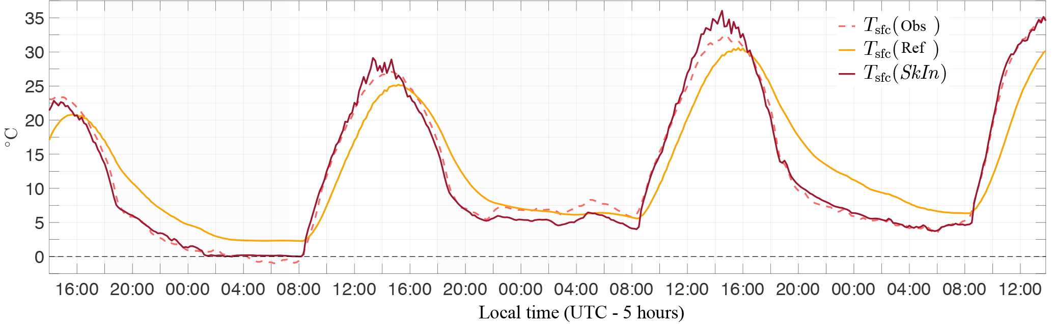
Figure 3 Performance of the JSBACH scheme on diurnal timescales: comparison of time series of the surface temperature (T_sfc) between the reference model (orange line) and SkIn (red line) plotted against observations (dashed line). Data are from the CASES-99 experiment in Kansas from 23 to 26 October 1999.

The surface temperature exhibits a similar phase shift (Fig. 3): in the reference simulation the surface temperature is underestimated by up to 4 K in the case of heating and overestimated by up to 8 K in the case of cooling with respect to the observations. The simulation of SkIn only shows some minor disagreement with the observations. In particular, SkIn overestimates the surface temperature maximum on the second and third day, but apart from that it fits the observation quite well. The behavior of the surface temperature in the reference run exhibits a phase shift, as it is equal to the soil temperature at about 3 cm depth. Here, the ground heat flux, as the heat exchange between the first and second soil layers of the reference run, shows the same inertial lagging (Fig. 2). In addition, it is quite smooth and overestimates the nightly ground heat flux (particularly on the first night). The same phase shift in temperature as well as the delayed response in the heat fluxes was also found by Betts et al. (1993).

Interestingly, the phase error with respect to the observations in the temporal course of the surface temperature caused by the dampening effect exerted by the heat storage exhibits an asymmetric behavior. The phase shift between the surface temperature and the observed temperature increases with time and is much larger during the night than during the day. In the SkIn scheme, the adjustment to an equilibrium temperature, which is determined by the radiative forcing, is achieved instantaneously, whereas in the approach that includes a heat storage the temperature difference between the simulated temperature and the equilibrium temperature decreases over time according to an exponential rate. The time required to reach the equilibrium state is determined by a time constant which depends on the turbulence conditions in the atmosphere. During the day the turbulent motions intensify the turbulent exchange and reduce the time needed to reach the equilibrium. In contrast, at night the exchange is strongly reduced under stable conditions resulting in longer relaxation times. As a result, the simulated temperature in the SkIn run is always lower than that in the reference run in the afternoon and during the night. Moreover, the skin conductivity like the drag coefficient – in contrast to the heat capacity – acts to reduce the relaxation time to reach the equilibrium. However, we agree that the incorporation of a skin conductivity as well as the drag coefficient also damps the amplitude of the response of the surface temperature to variations in the forcing. Overall, the conclusion can be drawn that, on the basis of a daily average, the cooling effect of SkIn outweighs its small warming effect during the day for regions where shallow vegetation prevails (here SkIn leads to a cooling of 0.6 K).

In the next section, this finding will be further examined using an AMIP experiment. Moreover, we will address the extent to which the surface processes of regions with tall vegetation or regions located at high latitudes without a pronounced diurnal cycle will respond to the formulation of the land–atmosphere coupling.

3.2 Results of the AMIP run

A key aspect of the SkIn⁺ scheme is the introduction of the canopy heat storage (S_cano). Since the latent heat storage (S_q) cannot be completely related to a temperature tendency, it is not possible to compare the heat capacities related to different processes; however, it is necessary to compare different heat storages. Because heat storages have the nature to compensate each other over longer timescales, we only compare positive contributions of the heat storages to estimate their magnitude. This could be interpreted as the average amount of energy that is stored in the canopy. The same amount will also be released. The 30-year mean of the canopy heat storage ranges between roughly 5 and 15 W m⁻² for high vegetation (Fig. 4, upper panel). The total canopy heat storage (S_cano) amounts to 3.7 W m⁻² in the global land mean. This value appears relatively small due to the fact that the regions with no or shallow vegetation account for negligible storages (around 0 W m⁻²) and do not contribute to the mean. The heat storage in the canopy air space (S_T) amounts to 19 % of the total canopy heat storage and the latent heat storage (S_q) constitutes 22 %. The most significant contribution to the total storage with around 60 % comes from the heat storage of the moist biomass (S_veg). In the warm and humid tropics, where high vegetation prevails, the largest values for the canopy heat storage are found. Here, the latent heat storage partly shows a similar magnitude to the biomass heat storage. In the tropics the total canopy heat storage averages 12 W m⁻² (15 W m⁻² at maximum), whereas in the taiga mean values of 5 W m⁻² are observed, and in deciduous forests mean values of 3 W m⁻² are found.

Figure 4 Comparison of canopy and soil heat storage: global distribution of the positive contributions of the canopy heat storage (S_cano) (a) and the soil heat storage (S_soil) (b), both in W m⁻² as a 30-year mean (1979–2008).

Comparing the latent heat storage (S_q) qualitatively on diurnal scales with the other two storage terms, which are directly related to the surface temperature tendency, we find that the temperature related heat storages tend to react like a common heat storage. A common heat storage exhibits a positive peak during the first half of the day and a negative during the second half of the day (compare the soil heat storage in Fig. 2), whereas the latent heat storage does not show this temporal course. It shows positive as well as negative changes in heat storage throughout the day. This corresponds to the fact that the specific humidity does not follow a strict diurnal pattern like the surface temperature. On the contrary, there are different kinds of days that represent either a positive or negative trend in humidity depending on dry or wet periods.

The positive part of the chemical heat storage ($\mathit{\beta }{F}_{{\mathrm{CO}}_{\mathrm{2}}}$) follows the same regional pattern as the other canopy heat storages whereas the temporal course on diurnal scales differs. In particular, the chemical heat storage follows the PAR (photo active radiation) part of the incoming solar radiation and results in energy consumption during the day and energy release due to respiration at night. With 0.64 W m⁻² on global average it amounts to 17 % of the total canopy heat storage (S_cano) and is slightly smaller than S_T. Nevertheless, it should not be neglected because the sum of all of these supposedly small terms could be important. As previously mentioned, we think that the chemical heat storage is an interesting process which should also be investigated in connection with the interaction between the carbon cycle and the climate on longer timescales.

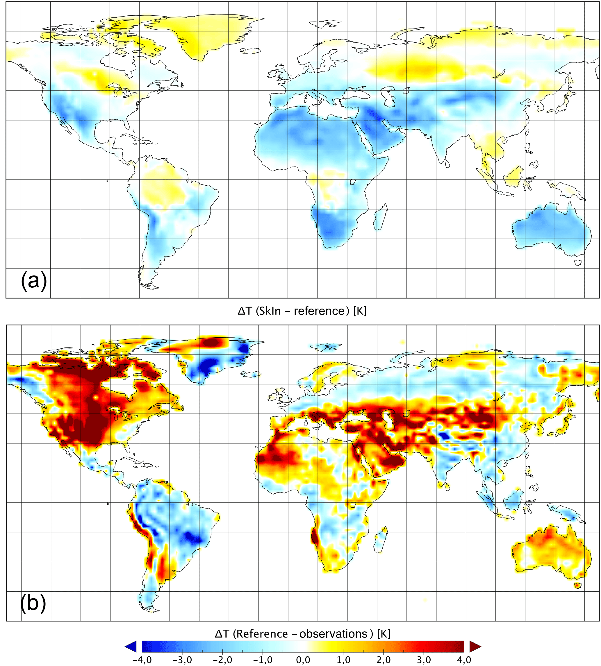
Figure 5 Performance of the SkIn⁺ scheme on regional scales: 30-year (1979–2008) summer season (April–September) average of the difference in near surface temperatures between SkIn⁺ and the reference run (a) as well as between reference run and observations (in short model bias, b).

The soil heat storage in the reference model (Fig. 4, bottom panel) is related to the soil heat capacity of the uppermost soil layer, which is determined by the present soil type based on the FAO soil classification guidelines. The soil heat storage varies spatially in the range between 5 and 50 W m⁻² and amounts to 17 W m⁻² on global average. For regions with tall vegetation it reaches values of about 10 W m⁻², which corresponds to the same order of magnitude as the canopy heat storage in the SkIn⁺ scheme: for tropical forest it is slightly smaller, and for Northern Hemisphere forests it is slightly larger. However, the soil heat storage significantly exceeds the canopy heat storage in regions with no or low vegetation. In general, the magnitude of the canopy heat storage as well as the soil heat storage is proportional to the temperature tendency. The regions with no or low vegetation exhibit the largest diurnal ranges in temperature. Therefore, the largest discrepancy appears in these areas and amounts to up to 50 W m⁻². Thus, we expect that the main influence of the SkIn⁺ scheme occurs in regions where bare soil or shallow vegetated regions dominate, such as grass lands or savanna, while we expect a rather small effect in forested regions.

Figure 5 illustrates the performance of the SkIn⁺ scheme, which includes the canopy heat storage (S_cano), on regional scales using a 30-year average for the summer season (April to September) (upper panel) by displaying the difference of the near surface temperature between SkIn⁺ and the reference run. Based on our experience with the offline version, we know that SkIn leads to a warming during the day and a cooling at night due to its instantaneous response to the radiative forcing. Thus, the sign of the local mean temperature difference between SkIn⁺ and the reference run depends on whether the night effect prevails or whether the daytime effect and other processes predominate, such as clouds and precipitation. In the global mean, SkIn⁺ leads to a cooling of 0.22 K. Almost all regions characterized by no or low vegetation and a pronounced diurnal cycle, where mostly well mixed conditions during the day and very stable conditions during the night occur, show an overall cooling in SkIn⁺ relative to the reference scheme (with a maximum of up to −3.5 K). This effect is clearly visible in Australia, the southwestern United States, the Gran Chaco region in South America, the Sahara, the Arabian region and central Asia.

In the tropics SkIn⁺ and the reference scheme show much smaller differences which suggest that the canopy heat storage in SkIn⁺ roughly corresponds to that of the uppermost soil layer. Only in some parts of the tropics is SkIn⁺ slightly warmer than the reference scheme, indicating an opposite SkIn effect, with higher temperatures at night and lower temperatures during the day. Consequently, an absence of the canopy heat storage would lead to a slight cooling in the tropics. With respect to the mid and high latitudes of the Northern Hemisphere, we note that north of 50^∘, SkIn⁺ leads to a warming in summer relative to the reference scheme because the daytime effect prevails in this region and is caused by the supply of heat during the longer insolation period in these regions during the Northern Hemisphere summer.

Figure 5 (bottom panel) depicts the difference in near surface temperatures between the reference run and the observations (WATCH dataset). A comparison of the patterns of the upper and the bottom panel in Fig. 5 shows that for certain regions, where the reference model tends to be too warm, SkIn⁺ produces a cooling and vice versa. Not all biases disappear entirely, especially as the existing biases are much larger than the effects due to SkIn⁺, but the SkIn⁺ scheme significantly improves the overall performance of the land surface exchange by reducing the model bias. Thus, the root mean square error of the global average temperature bias over land is reduced by 0.19 K, which corresponds to a bias reduction of about 9 %. SkIn⁺ leads to significant improvements in the southwestern United States, the Gran Chaco region, western and central Africa, and particularly in the Arabian region, central Asia, and Australia. In some other regions, such as parts of South Africa or in North America's boreal forests, the SkIn⁺ scheme seems to be unable to reproduce the temperature patterns. Therefore, further refinements are required to improve the treatment of various land–atmosphere interaction processes, in particular over boreal forests and in snow covered regions. Moreover, other biases that are not related to land processes, for example, those caused by the atmosphere and its large-scale circulation patterns, may be responsible for the apparent short comings of the SkIn⁺ scheme.

4 Discussion

In this study we demonstrate that the soil heat storage approach appears to be too simple and is unable to correctly reproduce the coupling between the land surface and the atmosphere with respect to the simulation of diurnal cycles of energy fluxes and the near surface temperature in regions with low vegetation. SkIn⁺ does not show an unambiguous effect in one direction but causes both cooling and warming depending on the time of day. It is debated that the heat storage approach only induces phase errors in the diurnal cycle of surface fluxes and of near surface temperatures producing errors that cancel each other when averaged over longer timescales. However, this assumption appears to be untrue because a temperature signal of up to 3.5 K is found in the 30-year temperature average differences. Moreover, the calculation of the correct timing of heat fluxes is an important issue per se because it influences and triggers convection, which governs the formation of clouds and precipitation and, in turn, affects the energy fluxes. Therefore, we recommend that the SkIn⁺ scheme should be used not only for models that operate on short timescales but also for Earth system models with longer timescales.

However, in some regions the SkIn⁺ scheme shows worse performance than its predecessor, likely because some existing biases only emerge in the SkIn⁺ scheme. In addition, we believe that the SkIn⁺ scheme, which considers the canopy heat storage, would take full effect in cases where subgrid scale surface temperature variations in a grid cell are taken into account. At the moment, the surface energy balance is solved for the whole grid box using the parameter averaging method implying that an identical surface temperature is assigned to the whole grid cell. A more promising approach, which would be more suitable for the SkIn⁺ scheme and would allow a better representation of spatial subgrid-scale heterogeneity, would be a flux aggregation method (Best et al., 2004; de Vrese and Hagemann, 2016). An example of the use of the flux aggregation method is the Tiled ECMWF Scheme for Surface Exchanges over Land model (Balsamo et al., 2009). Moreover, future developments of land surface exchange schemes should also take the vertical discretization of the thermal structure within the canopy layer into account, which is important in case of high vegetation. Here, the temperature of the tree crown, the surface temperature under the trees, the ambient air space temperature within the canopy, and the leaf temperature itself are differentiated (Vidale and Stöckli, 2005). The development of the SkIn⁺ scheme is only the first step to decoupling the surface energy balance from the soil layer. We believe that future studies, taking more processes within the canopy layer into account to address the role of the leaf temperature and its relation to the evapotranspiration within the forest, will be capable of improving our understanding of land–atmosphere exchange processes.

5 Conclusions

In several current climate models it is common practice to use a prognostic procedure to close the surface energy balance within the uppermost soil layer of finite thickness and heat capacity. In this study, a different approach was investigated by closing the energy balance diagnostically at an infinitesimally thin surface layer (SkIn). We addressed the question of whether the classic heat storage concept correctly reproduces the coupling between the land and the atmosphere throughout the diurnal cycle regarding shallow vegetation. Therefore, we performed an offline site experiment with JSBACH, the land component of the MPI-ESM, using observations from the CASES-99 field experiment in Kansas. Analyzing the surface energy balance in both schemes, we found the following:

• The heat storage in the standard scheme causes a dampening effect resulting in phase errors with respect to the time-dependent behavior of the heat fluxes and surface temperatures.

• A part of the stored energy is released during the night which unrealistically destroys the stable boundary layer.

• The surface temperature simulated with the reference scheme is underestimated in the case of heating during the day and overestimated in the case of cooling at night.

Here, we conclude that the SkIn scheme leads to significant improvements in the representation of exchange processes and removes almost all biases.

Following this, we investigated the effect of the SkIn scheme on longer time and larger spatial scales. The questions we addressed were whether the SkIn scheme shows a regional impact on longer timescales, and if so, whether the current biases in near surface temperature are at least partly caused by the former oversimplified parameterization of the surface energy balance. To answer these questions, a global coupled land–atmosphere experiment covering the years from 1979 to 2008 (AMIP run) with prescribed sea surface temperature was performed. For this global run, the standard heat storage concept is replaced by a physically motivated approach that describes the heat storage of the canopy layer in the surface energy balance (SkIn⁺). In this method, not only is the heat storage of the biomass itself taken into account, but the heat storage of the air and its humidity within the canopy layer is also included. In addition, we wanted to determine if the daily warming or the nightly cooling, which occurs in the offline site level version of SkIn, also prevails in the coupled run and if so which effect dominates in which region. Comparing the simulated summer near surface temperatures of the SkIn⁺ scheme with those of the reference run as well as with the WATCH data we find the following:

• The heat storage of the canopy layer must be taken into account in regions with tall vegetation (especially in the tropics). Here, the heat storage of the canopy layer is larger than that of the uppermost soil layer.

• The turbulent exchange during daytime counteracts the delayed response in near surface temperature, whereas during stable conditions at night a significant phase shift occurs.

• For most regions – especially those with no or low vegetation and a pronounced diurnal cycle – the night effect of SkIn⁺ prevails leading to a cooling in the near surface temperature relative to the standard scheme.

• For the tropics, where the heat storage of the canopy layer is larger than that of the uppermost soil layer the SkIn⁺ scheme leads to a slight warming.

• For high latitudes SkIn⁺ tends to warm the near surface air temperature due to the extended day length in the Northern Hemisphere in summer.

In summary, the SkIn⁺ scheme also shows a significant global effect on longer timescales and a reduction of the model bias in several regions.