the Creative Commons Attribution 4.0 License.
the Creative Commons Attribution 4.0 License.
 | 24 Aug 2018
The microscale obstacle-resolving meteorological model MITRAS v2.0: model theory
Mohamed H. Salim
K. Heinke Schlünzen
David Grawe
Marita Boettcher
Andrea M. U. Gierisch
Björn H. Fock
This paper describes the developing theory and underlying processes of the microscale obstacle-resolving model MITRAS version 2. MITRAS calculates wind, temperature, humidity, and precipitation fields, as well as transport within the obstacle layer using Reynolds averaging. It explicitly resolves obstacles, including buildings and overhanging obstacles, to consider their aerodynamic and thermodynamic effects. Buildings are represented by impermeable grid cells at the building positions so that the wind speed vanishes in these grid cells. Wall functions are used to calculate appropriate turbulent fluxes. Most exchange processes at the obstacle surfaces are considered in MITRAS, including turbulent and radiative processes, in order to obtain an accurate surface temperature. MITRAS is also able to simulate the effect of wind turbines. They are parameterized using the actuator-disk concept to account for the reduction in wind speed. The turbulence generation in the wake of a wind turbine is parameterized by adding an additional part to the turbulence mechanical production term in the turbulent kinetic energy equation. Effects of trees are considered explicitly, including the wind speed reduction, turbulence production, and dissipation due to drag forces from plant foliage elements, as well as the radiation absorption and shading. The paper provides not only documentation of the model dynamics and numerical framework but also a solid foundation for future microscale model extensions.
- Article
(3007 KB) - Full-text XML
- BibTeX
- EndNote


The urban boundary layer is considerably influenced by its surface characteristics. Within the canopy layer, atmospheric flow is disturbed by buildings and other obstacles located at the surface and hence all related atmospheric processes (Meng, 2015). This creates a complex three-dimensional, time-dependent flow, temperature, and humidity field. Studying the atmospheric boundary layer flow and its interactions with complex terrain in, e.g., urban areas is a complex problem for both the meteorological and engineering communities. Field experiments are one approach (e.g., Schafer et al., 2005); however, field measurements have a low spatial representativeness and largely depend on the turbulence structure within the urban area and the wind direction fluctuations. This implies that long averaging times are needed in order to obtain reasonable time-averaged values; on the other hand, long averaging times are not feasible because the atmospheric situation changes due to, e.g., the diurnal cycle or synoptic changes. Also, investigating future scenarios is not possible from field measurements. Subsequently, laboratory experiments in controlled conditions (wind tunnel) are used to overcome these problems after matching the major similarity parameters with the full-scale model. These physical models can be very detailed (Harms et al., 2011) and can provide comparison data for numerical models and field experiments (VDI, 2015). However, wind tunnel modeling is mostly limited to neutral atmospheric stratification due to the requirement of similarity to nature. Furthermore, it is sometimes difficult to satisfy the atmospheric boundary conditions and to resemble important features of the Earth system such as the Coriolis force effect. Alternatively, high-resolution numerical computer models are frequently used to simulate urban areas.
Numerical modeling of wind flow and pollutant dispersion in urban areas is a challenging task due to the geometrical variety of buildings. It inevitably involves impingement and separation regions, a multiple vortex system with building wakes, and jet effects in street canyons (Murakami et al., 1999). Furthermore, the neighbor buildings add their own impacts on the urban meteorology, resulting in interacting flow and dispersion patterns. Due to this complexity, explicit resolving of the buildings is necessary instead of only implicitly considering building effects by using surface roughness parameterizations. This gave rise to the development of obstacle-resolving microscale meteorological models such as PALM (Maronga et al., 2015), ASMUS (Gross, 2012), ENVI-met (Bruse and Fleer, 1998; Müller et al., 2014), MISKAM (Eichhorn, 1989; Eichhorn and Kniffka, 2010), MUKLIMO (Früh et al., 2011), MITRAS (Schlünzen et al., 2003; Salim et al., 2011), and OpenFOAM (Franke et al., 2012). These models are now widely used for environmental and engineering studies.
The microscale obstacle-resolving transport and stream model MITRAS is part of the M-SYS model system (Trukenmuller et al., 2004; Schatzmann et al., 2006). This model system is designed to investigate pollution transport, chemical reactions, and atmospheric phenomena in the atmospheric boundary layer. The obstacle-resolving MITRAS model calculates wind, temperature, humidity fields, cloud, and rainwater, as well as tracer transport within the obstacle layer. The model has been applied for more than 10 years; however, an overall description of the model theory has not been published in a refereed journal. This is timely because computers now allow for time-dependent long-term integration of the temperature and humidity equations in high resolution. In addition, MITRAS in its version 2 was extended and optimized for more realistic applications in urban areas (Salim et al., 2011; Röber et al., 2013). Specifically, more surface cover classes were added to better describe surface characteristics: fine tuning the code structure for maximum parallelization to make it faster and able to simulate larger domains and parameterizing the additional radiation, turbulence production and dissipation due to wind turbines, and urban vegetation.
Model validations of MITRAS-01 have been performed in comparison to wind tunnel data (Schlünzen et al., 2003; Grawe et al., 2013). MITRAS 2 is evaluated using the VDI guideline for obstacle-resolving microscale models (Grawe et al., 2015). The results will be presented in a separate paper.
Equations and the solution method will be described in Sect. 2, including the turbulence parameterization (Sect. 2.2) and numerical treatment (Sect. 2.3). Further sub-grid-scale processes need to be parameterized, even in a very highly resolving atmospheric model like MITRAS. This concerns cloud microphysical processes and radiation. Both are calculated with the same parameterizations as its sister model METRAS (Schlünzen, 2003; Schlünzen et al., 2018b). The boundary conditions, including surface, lateral, and top boundaries, are given in Sect. 3. The treatment of obstacle-induced effects is described in Sect. 4, including wind, shading, and heat transfer effects. MITRAS parameterizes momentum and heat fluxes on obstacle surfaces dependent on the local roughness length (Sect. 4.1, 4.2) and explicitly resolves obstacles such as buildings, including overhanging obstacles (e.g., bridges or overpasses), trees, and wind turbines, to account for its aerodynamics and thermodynamic effects. The handling of wind turbines in the model and their effects is described in Sect. 4.3. Vegetation effects, especially their effect on radiation, are given in Sect. 4.4.
2.1 Model equations
MITRAS is based on the physical conservation equations, specifically the Navier–Stokes equations, the continuity equation, and the conservation equation for scalar quantities such as potential temperature and humidity. This set of equations is written in flux form, transformed in a terrain-following coordinate system and filtered before it is used in MITRAS.
2.1.1 Coordinate transformation
The equations of MITRAS in flux form are transformed in a three-dimensional nonuniform terrain-following coordinate system , , so that the lower boundary conforms to the terrain. The vertical coordinate is defined by
Here zs(x,y) is the orography height and zt is the domain height. The terrain-following coordinates ensure an easy specification of the boundary conditions over orography and eases nesting of MITRAS in METRAS due to the use of the same vertical coordinate transformation. The transformation used allows for grid stretching in all three directions to keep a high resolution in the focus area of the domain while allowing some distance between the open boundaries (lateral and top) and the area of interest. In addition, the coordinate system can be rotated against north in any desired angle, allowing for additional flexibility. Figure 1 shows an example of a vertical cross section in this terrain-following coordinate system.

Figure 1Vertical cross section to illustrate the MITRAS grid in the terrain-following coordinate system (not to scale). The blue blocks denote buildings. Not all grid cells are shown.
2.1.2 Filtering of equations, basic state, and approximations
Reynolds averaging is used to filter the equations after the coordinate transformation: the atmospheric state variables are divided into a value , which is the average over a finite time, Δτ, and grid volume, , and its deviation ψ′ (Pielke, 2002). The deviations are assumed to be zero when averaged over Δτ. This assumption is reflected in the choice of parameterizations for sub-grid-scale (SGC) turbulent fluxes (Sect. 2.2). Performing the filtering operation after the coordinate transformation ensures that all possible fluctuations are included with their correct contravariant and covariant components. The average is further decomposed for temperature, humidity, concentration, pressure, and density into a large-scale part ψ0, the so-called basic state, and a microscale deviation . The basic state is intentionally chosen to be steady state and fulfill basic concepts of meteorology. For example, the base state pressure p0 is chosen so that it satisfies the hydrostatic approximation and the vertical gradient is thus balancing gρ0. This ensures a higher order of accuracy when solving the equations, especially for the vertical wind. ψo represents a domain average value using the values at the same height above sea level:
where ya and xa are the coordinate of a corner of the model and δxδy the domain size in the x and y direction.
To increase the numerical accuracy further, the pressure deviation, , is decomposed into a quasi-hydrostatic pressure p1 (in balance with ) and a more or less dynamically impacted part p2, i.e., . So the pressure can be expressed as . Here so p′ is neglected.
The Boussinesq approximation is used, and thus density variations in the Navier–Stokes equations are neglected except for the buoyancy term. p2 is determined from an elliptic differential equation, which is derived from the anelastic approximation of the continuity equation, resulting in a decoupling of pressure and density in the model and hence no sound wave propagation. In addition to the above equations, the ideal gas law and the equation for the potential temperature are solved diagnostically to couple the thermodynamic and aerodynamics of the model.
2.1.3 Solved equations
The solved prognostic equations in MITRAS are as follows.
Here , , and are the wind velocity components in the Cartesian coordinates, is the contravariant vertical component of the wind vector, α∗ denotes a grid volume, (, , , and (x, y , z) are the coordinates of the terrain-following coordinate system and of the Cartesian system, respectively. Ug, Vg denote the horizontal components of the geostrophic wind, sources and sinks of . The Coriolis parameters f and are calculated according to the local geographic latitude ϕ and the angular velocity of the Earth's rotation Ω as f=2Ωsinϕ and . The variables d=sinξ and account for the rotation of the coordinate system by an angle ξ against north. The terms , , , and are the sub-grid-scale (SGS) turbulent momentum and scalar fluxes emerging from filtering the equations. Subscript notation for the coordinate transformation terms is used.
2.2 Parameterization of turbulent fluxes
2.2.1 Closure for momentum fluxes
Due to the filtering, sub-grid-scale (SGS) fluxes arise. The three SGS turbulent fluxes in the momentum equations (j=1, 2, 3) are
The SGS fluxes can be expressed in terms of the Reynolds stress tensor τij, which is related to the deformation tensor through the turbulent mixing coefficient (Lilly, 1962; Smagorinsky, 1963).
At the lowest model layer, the validity of Monin–Obukhov surface layer similarity theory (Monin and Obukhov, 1954; Foken, 2006) is assumed. The grid-box-averaged values of u∗, θ∗, qv∗ are calculated using stability functions of Dyer (1974) with von Karman constant κ=0.4.
Above the lowermost model layer the SGS turbulent fluxes are derived from a first-order closure (Detering, 1985; Etling, 1987).
Kij is the turbulent exchange coefficient for momentum in the xj direction. The last term in Eq. (8) represents the reduction of the diagonal fluxes due to pressure. Since this term is small compared to the deformation tensor term, it is neglected in MITRAS. Due to the symmetry of τij, the actually calculated exchange coefficients are only a horizontal exchange coefficient (Khor) and a vertical exchange coefficient (Kvert).
2.2.2 Closure for fluxes of scalar quantities
The turbulent fluxes for scalar quantities, e.g., potential temperature, are expressed as
These fluxes are also parameterized by a first-order closure.
Kiχ is the corresponding mixing coefficient in the xi direction, which is related to Kij.
The exchange coefficients in MITRAS are either calculated using the Prandtl–Kolmogorov closure (Sect. 2.2.3, first subsection) or the E–ε turbulence closure (Sect. 2.2.3, second subsection). In both turbulence closures the exchange coefficients are calculated as a function of the SGS turbulent kinetic energy E, for which an additional prognostic equation similar to Eq. (6) is solved. For the E–ε turbulence closure the dissipation ε is additionally calculated from a prognostic equation (López et al., 2005).
2.2.3 Exchange coefficients calculation
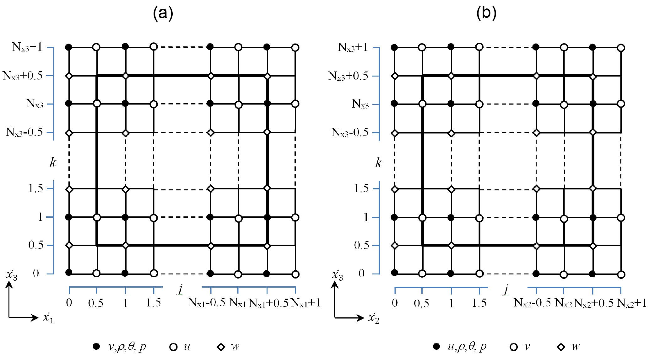
Figure 2Sketch showing the staggering of the variables of a domain in (a) the x–z direction and (b) y–z direction for a model domain with size . The thick line denotes the model domain boundaries. For simplification a uniform grid is shown.
Prandtl–Kolmogorov closure
The exchange coefficients are calculated as follows.
c1 is a free constant determined by matching the theoretical model against experimental values. It has the value 0.55 in MITRAS (López, 2002). The Richardson number Ri-dependent term is defined as
and in accordance with the stability functions used in the surface layer. For the SGS turbulent kinetic energy, E, a prognostic equation is solved. The dissipation rate ϵ is calculated diagnostically as
cε is a constant set to 0.166 (López, 2002). The local mixing length l is related to the stability function φm and the distance to the nearest solid surface zw, which can be the ground surface or a surface of a resolved obstacle. The equation of l reads
λ is the maximum eddy size (a value of 100 m is used).
E–ε turbulence closure
This closure is based on the standard E–ε model and the Kato and Launder (1993) modifications, which eliminate the excessive turbulent kinetic energy produced by the standard E–ε model in stagnation regions (López et al., 2005). The mechanical production term PM in the E equation can be derived according to the Kato and Launder (1993) modifications as
S is the dimensionless strain rate.
Ω is the rotation rate:
which goes to zero near the stagnation point, so PM is significantly reduced.
It has been shown by Schlünzen et al. (2003) that using Kato and Launder (1993) modifications for both the turbulent kinetic energy equation and the dissipation equation in MITRAS leads to overestimation of the momentum fluxes at the stagnation point. To overcome this drawback, they suggested limiting the Kato and Launder reformulation to the energy equation only. So, for the ε equation, the PM term is calculated the same way as in the standard E–ε model.
The buoyancy term is calculated in the same way as in the Prandtl–Kolmogorov closure. The values for the constants c1, c2, cμ are taken as suggested by López (2005) as cμ=0.09, c1=1.44, c2=1.92.
2.3 Numerical solution
2.3.1 Discretization
The model equations are solved using finite-volume methods on a staggered Arakawa C grid (Arakawa and Lamb, 1977). On this grid, scalar variables are defined at the cell center, while the velocity components are defined on their respective normal cell faces (Fig. 2). The obstacles faces are set where the corresponding wall normal velocity components are defined. Since u, v, w, and the scalar variables are defined at different locations in space, four index arrays are needed to describe the obstacle in the discretized 3-D model domain. The discretization allows for grid stretching in both the vertical and horizontal directions to keep focus on the inner part in the domain. The scalar points are always in the center of a grid cell, while the wind components might have different distances to the next-neighbor scalar grid point.
2.3.2 Numerical scheme
The advection and diffusion terms in the momentum equations are solved in MITRAS using the Adam–Bashforth scheme in time and centered differences in space. The vertical diffusion terms are determined using the Crank–Nicholson implicit scheme in order to increase the time step for vertical exchange processes. All other terms in the momentum equations except dynamic pressure p2 are solved forward in time and centered in space.
The dynamic pressure p2 is determined iteratively from a Poisson equation to satisfy the anelastic approximation. MITRAS allows two user-selected options for the iterative procedures, the iterative IGCG scheme (idealized generalized conjugate gradient; Kapitza and Eppel, 1987) and the preconditioned BiCGStab method (biconjugate gradient stabilized; Van der Vorst, 1992).
To avoid numerical artifacts that might appear due to nonlinear interactions and result in shortwave energy accumulation, artificial diffusivity is added.
The advection of scalar quantities is solved forward in time and using the upstream scheme for advection. Even though the upstream method is known for being diffusive with its implicit diffusivity Knum in, e.g., the x direction given by (Roache, 1982), the artificial diffusivity is acceptable in the target area of the domain for two reasons. (a) The isotropic grid and building impacts ensure advection and diffusion in the horizontal and vertical direction being of comparable size, and (b) advection is often larger than diffusion terms since the SGS turbulence is small within the canopy layer. U is the local wind speed, Δx is the local grid width, and Co is the Courant number.
Since Eq. (13) implies that dissipation rate and sub-grid-scale turbulent kinetic energy are directly coupled, the dissipation cannot be calculated with very large time steps. Equation (13) is solved by determining an analytic solution (Appendix A) as suggested by Fock (2015). This avoids unphysical values of ε, which might even be negative for large time steps Δt.
In MITRAS, several types of boundary conditions can be used in physically consistent combinations to allow for different kinds of simulations. At the ground surface (lower boundary) and obstacle faces (Sect. 4) material interfaces are given, while the lateral boundaries and the upper boundary are artificial due to the use of a limited area model.
3.1 Surface boundary
3.1.1 Wind velocity
For the horizontal wind velocity components, a no-slip boundary condition (, j=1, 2) is used at all vertical surfaces. With this the vertical wind defined in the staggered grid at the surface also results in zero. Since u and v are defined at the lowest level at k=0.5 (Fig. 2) on the staggered grid, a Neumann boundary condition is used with a constant gradient using the zero surface values. With this the no-slip condition is achieved at the surface. Additional details for buildings are given in Sect. 4.1.
3.1.2 Dynamic pressure (p2)
The boundary condition for the pressure p2 is formulated by considering the wind velocity boundary condition, the grid staggering, the position of the domain boundaries, and the dynamic pressure equation. Consistent with the no-slip boundary condition, the boundary condition used for p2 at the wall is
Due to the terrain-following coordinate system (Eq. 1) the vertical gradient of the dynamic pressure p2 needs to be zero perpendicular to the surface.
3.1.3 Temperature
The calculated temperature values of all physical boundaries (ground and obstacles surfaces, i.e., wall and roof) are used at the lower boundary and at the obstacle surfaces. The necessary additions for buildings are provided in Sect. 4.2. These temperature values are calculated using the force-restore method for the ground soil heat flux. Following Tiedtke and Geleyn (1975) and Deardorff (1978), the temperature at the surface, , is calculated as
H is the force term of the fluxes of the surface energy budget: the net shortwave (RSW,net) and longwave radiation flux (RLW,net), the sensible (QS) and latent heat flux (QL), and the anthropogenic heat emission flux (Qa). is the deep soil temperature, hθ represents the depth of the daily temperature wave in the restore term, and κs is the thermal diffusivity of the surface cover material.
Both RSW,net and RLW,net are calculated using the atmospheric radiation scheme of the MITRAS sister model METRAS (Schlünzen et al., 2018b) and the surface characteristics, i.e., the albedo value. The influence of vegetation and the shading from the obstacles is taken into account in the calculation of radiation (Sect. 4.4). The fluxes QS and QL are calculated with respect to the thermal stratification using the friction velocity u∗ and the scaling values for heat, θ∗, and water vapor, q∗.
For obstacles, the calculated surface temperature (Sect. 4.2) of the obstacle surfaces is used at the corresponding grid cells.
3.1.4 Humidity
The following budget equation, introduced by Deardorff (1978), is used to calculate the humidity at the lower boundary (.
αq is the soil water availability, is the saturated humidity at , and is the specific humidity at the first model level. The initial value of αq is given for each surface cover class (Sect. 5.2). A prognostic equation is used to calculate αq in the time-dependent model integration.
QE is the turbulent humidity flux at the surface (calculated in consistency with QL), J kg−1 is the latent heat of vaporization of water, P is the precipitation (if any), ρw water density, and Wk is the saturation value for water content. This is prescribed for each surface cover class (Sect. 5.2).
3.1.5 Other scalar quantities
At the ground surface and at the obstacle surface and ε are calculated as a function of local friction velocity, as follows.
The empirical constant c1 is set to the same value as in Eq. (11). This helps together with Eq. (12) to obtain continuous fluxes at the top of the lowest model cell, which employs the surface layer scheme (Lopez, 2002; Fock, 2015).
3.2 Lateral boundary
3.2.1 Wind velocity
Dirichlet boundary conditions are used in two different formulations. They can be used in MITRAS in arbitrary combinations to describe the lateral boundaries of the domain: open boundary (radiative) and fixed boundaries. The appropriate combination of boundary value calculations depends on the application. For instance, a realistic application with comparison to field data in mind needs open boundaries. In these the boundary normal wind components are calculated as far as possible from the prognostic equations. The boundary normal advection is treated with the use of the Orlanski condition at inflow boundaries and by the upstream scheme at outflow boundaries. For the boundary parallel velocity components a zero-flux condition is assumed (Schlünzen, 1990).
When comparison with wind tunnel measurements (e.g., Grawe et al., 2013b) is performed, fixed boundaries are advantageous. In these the wind profiles are to be imposed at the inlet boundary and kept fixed at the initial values, while at the outflow the wind velocity is treated as an open boundary.
3.2.2 Other variables
The normal gradients of pressure p2, temperature, humidity, and concentrations are set to zero at the lateral boundaries.
3.3 Top boundary
3.3.1 Wind velocity
For the vertical wind, which is defined at the model top, the Dirichlet condition is used, prescribing it to initial values (mostly vertical wind zero). For all other variables a Neumann boundary condition is employed for which the gradients normal to the boundary are zero. In order to avoid reflections of vertically propagating waves at the upper model boundary, Rayleigh damping layers (absorbing layers) are used in MITRAS. The Rayleigh damping terms, which are added to the flow equations (Eqs. 3–6), are written here.
Ug and Vg are the geostrophic wind velocity components and vR is the relaxation coefficient, defined as
k denotes the vertical grid point index, kt the index of the highest grid point at the upper boundary, and kD the index of the first absorbing layer. The coefficient δ is set to 0.2 and, based on our experience, five damping layers are sufficient.
3.3.2 Other variables
The normal pressure gradient, temperature gradient, turbulent momentum fluxes, and their gradients are all set to zero at the upper boundary. This assumption results in zero vertical heat and moisture fluxes as well as zero momentum fluxes at the upper model boundary.
4.1 Buildings
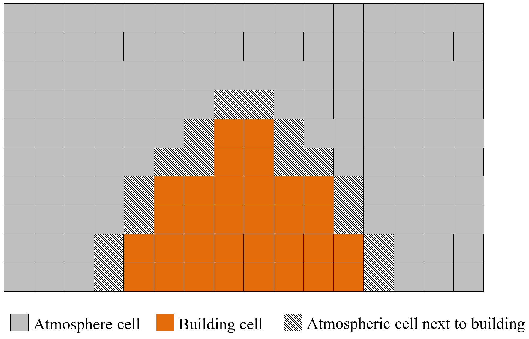
The concept of the mask method (Briscolini and Santangelo, 1989) is employed in MITRAS to explicitly resolve the buildings within the 3-D model domain. This method is based on the immersed boundary method (Mittal and Iaccarino, 2005), which allows for flow simulation in the vicinity of complex geometries that do not conform on Cartesian grids. Impermeable grid cells at the building positions are defined using 3-D fields of weighting factors, vol(, defined at each grid cell to give information about whether a grid cell is an atmospheric cell or a building cell (which lies mostly or completely inside a building). Any faces of a grid volume that are a wall or roof of a building are marked. This means that the grid cells in a domain are divided into three groups: grid cells in the free atmosphere surrounded by atmosphere without any adjacent building, grid cells next to building surfaces, and grid cells within buildings, as shown in Fig. 3. This separation facilitates the model coding and economizes the computational requirements.
A building mask containing these data is prepared by the preprocessor GRIMASK (Sect. 5.3). In the model, e.g., the wind velocity components vanish at the building boundaries by multiplying the fluxes with the face markers (impermeable walls). Additional wall functions are included to address friction effects properly.
Building surfaces influence the ambient air temperature. Their effect is taken into account by simulating the sensible heat flux. In grid cells that are adjacent to building surfaces, the term Qθ is added to the turbulent fluxes of heat (Eq. 9).
represents the temperature flux, which is calculated from the friction velocity at buildings, , and the scaling value for potential temperature, θb*. is calculated following the approach of Lopez (2002) as
assuming a logarithmic wind profile with neutral stratification over the building surface. |vb| is the wind speed parallel to the building surface at the first scalar grid cell next to the building surface, i.e., in the distance db. zb,0 is the roughness length of the building surface. The scaling value for potential temperature at buildings is calculated as
from the difference of the building surface temperature, θb, and the temperature at the first grid cell next to the building, θd,b. The roughness length for temperature at the building ( depends on the Reynolds number, Re. Following Brutsaert (1975), the roughness length ratio is calculated as
with the Prandtl number (Pr) set to 0.71.
This concept allows for a consideration of not only surface-mounted buildings but also overhanging obstacles such as bridges and overpasses or pathways to courtyards. They can all be considered in complex urban geometries.
4.2 Building surface temperature
In order to obtain an accurate surface temperature of the buildings (obstacles), most exchange processes at the building surfaces are considered in MITRAS, including turbulent and radiative processes (Gierisch, 2011). Thus, the physical properties of the façade and wall materials are to be introduced as model inputs. These properties include reflectivity, emissivity, heat transfer coefficient, and specific heat capacity.
The surface temperature of a building surface, Tb, is calculated from the energy budget of the infinitely thin outermost slab of the building façade. The slab is heated or cooled from outside by a heat source H and supported from inside by the rest of the façade that is connected to the building interior. The latter is assumed to be maintained at a temperature Tin.
The rate of temperature change of the slab is governed by the imbalance between the forcing term H and a restoring term. The prognostic equation for the surface temperature reads
Here the forcing term H is calculated from
RSW,abs and RLW,abs are the absorbed incoming shortwave and longwave radiation, QS and QL are the sensible and latent heat fluxes at the surface, which are calculated from the local friction velocity and the local scaling values for temperature and humidity (Gierisch, 2011), λ is the thermal conductivity, D is the wall thickness, and cwall is the wall volumetric heat capacity.
The surface energy balance for the inside wall surface can be written as
hi is the heat transfer coefficient for the internal wall, QC the heat conduction flux through the wall calculated as , and is the room temperature.
From Eq. (34), the relation between and is
Substituting for H and in Eq. (32) yields
The right-hand side of Eq. (36) is a function of . Thus
Solving Eq.(37) numerically,
and solving for gives the time-dependent equation for the surface temperature:
4.3 Wind turbines
Wind turbines are represented in MITRAS by impermeable grid cells at the position of the tower and the nacelle, similar to other buildings (i.e., vanishing wind speed and zero turbulent kinetic energy are assumed at grid points within the tower and nacelle). The orientation of the nacelle changes in relation to the wind direction during the model simulation. The wind turbine rotor is parameterized by using the actuator-disk concept (Molly, 1978; Mikkelsen, 2003; El Kasmi and Masson, 2008). In this concept the rotor is replaced by an imaginary permeable disk subjected to a distribution of forces that acts upon the incoming flow at a rate defined by the period-averaged kinetic energy that the rotor extracts from the atmosphere.
According to the actuator-disk model, the reduction of the wind speed is caused by the rotor thrust, T, which is formulated as
V1 is the speed of the approaching flow at wind turbine level, A is the rotor area, ρ is the air density, and cT is the nondimensional thrust coefficient for the corresponding wind speed. The wind speed deficit is limited to those cells located at the actual rotor position. The speed of the approaching flow is calculated with respect to the orientation of the rotor, which depends on wind direction and changes direction during the simulation. The thrust coefficient depends on wind speed and therefore the wind turbine automatically switches on and off in MITRAS at the cut-in and cutoff wind speed, respectively.
This wind turbine rotor blades create wake vortices of the wind turbines, which are associated with increased turbulence intensity. The turbulence generation in the wake is parameterized in MITRAS by adding an additional term, Qwt, to the turbulence mechanical production, PM, in the turbulent kinetic energy equation to account for the turbulence generation at the rotor position. This term is formulated as
uwt is a scale velocity used to characterize the turbulence. The factor cwt (s−1) includes the wind turbine characteristics that govern the amount of produced turbulence, namely the rotor size, the number of blades, and the rotational speed.
In MITRAS, the tangential velocity vθ, which is frequently used to model the vortex developing behind an aircraft, is used as the scale velocity. The Rankine vortex model (Gerz et al., 2001) is applied here to calculate vθ.
rc is the vortex core radius and ΓO is the rotor circulation, which is related to the rotor rotational speed, lift coefficient, and aspect ratio. More details about modeling the wind turbines in MITRAS are given in Linde (2011).
4.4 Vegetation
There are two modes of vegetation treatment in MITRAS: the implicit mode and the explicit mode. In the implicit mode, the effect of the vegetation (grass, bushes, trees, etc.) is implicitly considered in the surface parameterization using the roughness length. This is done by allocating the vegetation surface cover class for the corresponding surface grid cells and using the corresponding input parameters (e.g., roughness length, soil water, content, etc.; Sect. 5.2).
In explicit mode, vegetation effects are explicitly resolved. These effects include wind speed reduction (Schlüter, 2006), turbulence dissipation due to drag forces from plant foliage–atmosphere interaction (Salim et al., 2015), and radiation absorption and shading.
The wind speed reduction is parameterized by introducing a local three-dimensional sink term, , with i=1, 2, and 3 for the u, v, and w component. is added to the momentum equations (Eqs. 3–5). Following Liu (1996), the sink term is calculated as
Here cd is a drag coefficient, U is the mean wind speed at height , and LAD( is the equivalent leaf area density of the plant at height . The value of cd=0.2 determined by Katul (1998) is chosen here.
represents a source of turbulence due to the extraction of mean kinetic energy, , from the flow. However, the typical effect of vegetation is to reduce the overall turbulence by enhancing the dissipation of turbulence. To parameterize the additional turbulence creation and dissipation, additional source terms are added to the turbulent kinetic energy and dissipation equations. Following Wilson (1988) and Liu et al. (1996) these terms read as follows.
The reduction of the shortwave radiation flux is considered by including local reduction coefficients (ranging from 1 to 0) according to the vegetation characteristics. The reduction coefficients are described in terms of the vertical leaf area index, LAI, of the plant (see Sect. 5.4).
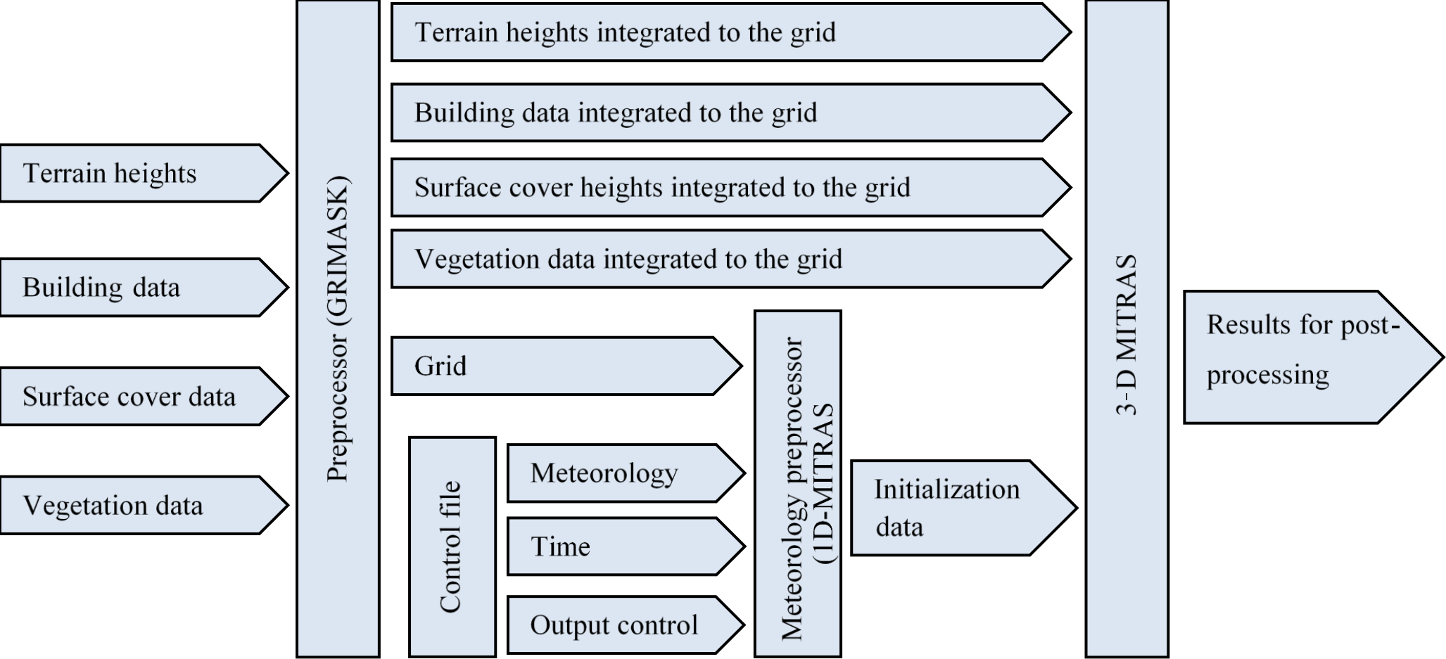
Several model inputs are required to run MITRAS to accurately simulate a domain for, e.g., an urban area (Fig. 4). These include, for instance, the orography heights of the domain, the surface cover types, the building data (dimensions, shape, and position), and the vegetation data for such a domain. Integrating these inputs to the computational domain of MITRAS is done in a separate preprocessor called GRIMASK (Salim, 2014). A complete description of this preprocessor is outside the scope of this paper, but the required input data and how they are in general achieved is outlined here (Sect. 5.1–5.4). Moreover, the representative meteorological conditions for the domain are required as inputs to run MITRAS; they are provided in consistency with the model physics and numeric using a preprocessor.
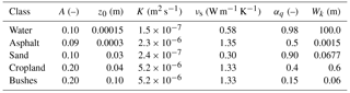
Table 1The physical parameters for some surface cover classes as used in MITRAS: albedo (A), roughness length (z0), thermal diffusivity (K), thermal conductivity (νs), soil water availability (αq), and saturation value for water content (Wk).
5.1 Orography height
Urban domains might include elevated terrain. To better describe the domain terrain, the orographic effects of the domain are considered in MITRAS by virtue of the terrain-following coordinate system (Sect. 2.1). Both the aerodynamic and the radiative (shading) effects of the slopes are considered in MITRAS. For realistic applications, the orography data (terrain height above sea level) of the domain are introduced to GRIMASK in the standard ASCII grid format of a geographic information system (GIS). Usually these data are in much finer resolution (less than 0.25 m) compared to the computational domain horizontal resolution (∼1 m). GRIMASK then aggregates these data to the surface grid cells to calculate the average orography height for each surface grid cell. This is done by splitting each grid cell into n sub-grids and calculating the orography height of each sub-grid. The eventual orography height, zs, of a grid cell (i,j) is calculated from
zsub(x,y) is the orography height of a sub-grid.
For idealized studies and test cases, GRIMASK can generate artificial orography heights according to the objective of the test case, e.g., a bell mouth hill or a Gaussian hill.
5.2 Surface cover
It is essential to define the surface cover characteristics of the urban domain because they govern the surface energy budget (Eq. 19) and all surface-dependent fluxes. In realistic cases, the urban domain usually contains several surface cover types (water, sealed surfaces, vegetation, sand, ice, etc.) and it becomes imperative to define an appropriate data structure to encode information on surface cover characteristics. To this purpose, the surface cover data are first introduced to GRIMASK in the GIS standard ASCII grid format. GRIMASK then integrates these data into the computational grid cells at the surface. Each grid cell is composed of at least one surface cover class, but more SGS surface covers are allowed. The preprocessor calculates how many surface cover classes exist in the domain and the portion of each surface cover class in each grid cell. This is done following the approach used to calculate the orography heights. Each grid cell at the surface is divided into sub-grids and the surface cover class of each sub-grid is defined. The data structure of the surface cover consists of two datasets: (a) the portion of each surface cover class in each grid cell and (b) a list of surface cover classes existing in the domain. Several classes are also prepared in the surface cover class database for the different vegetation types (coniferous trees, deciduous trees, bushes, etc.). A database of several surface cover classes with attributed physical parameters is available in the 1-D MITRAS model. The physical parameters given per surface cover class include albedo (A), roughness length (z0), thermal diffusivity (K), thermal conductivity (νs), soil water availability (αq), and saturation value for water content (Wk). The physical parameters are given in Table 1 for selected surface cover classes.
For buildings the explicit treatment is normally chosen. If the implicit consideration of obstacles is chosen, i.e., they are not explicitly resolved in the model grid, a much larger roughness length would be required, which conflicts with a high vertical grid resolution. This is similarly true for trees. The roughness length for water is modified during the model calculations with dependence on wind speed (Fischereit et al., 2016). The roughness length of scalar quantities over water, z0a, is calculated dependent on the roughness length for momentum, z0 (Brutsaert, 1975, 2013),
for temperature and humidity by substituting Ca with the Prandtl number Pr=0.76 and the Schmidt number Sc=0.6, respectively.
To distinguish surface cover classes, water, buildings, and sea ice, identifiers are incorporated for each surface cover class. These act as the Kronecker delta function to mark the particular class.
5.3 Building data
In order to generate the building mask used to provide the building data to the model, detailed information about the buildings in the domain is required. For instance, the building dimensions, shape, and location are needed for each building located in the domain to calculate the 3-D array volume and the building wall-based markers discussed in Sect. 4.1. This process is done in the preprocessor, GRIMASK, which allocates the buildings to the computational grid.
Since in the current version of MITRAS the 3-D field volume can be either 0 (building cell) or 1 (atmosphere cell), buildings are approximated to fit into the grid. For grid cells that are partially filled with buildings, the determination of whether these cells are building or atmosphere cells depends on how much volume of the cell is filled with building. A grid cell is considered a building cell if at least 50 % of its volume contains building. Otherwise it is counted as an atmosphere cell. This approximation is computationally efficient to consider the effect of buildings since the model equations only need to be multiplied by the 3-D field volume.
For realistic applications, complex urban building geometry can be provided to GRIMASK in either the raster digital elevation model (DEM) format, which is commonly used due to the advances in remote sensing technologies, or in the ASCII 3-D computer-aided design (CAD) format. GRIMASK integrates the high-resolution DEM data, which is a grid of squares representing the elevation of each small grid, to the computational grid and calculates how much volume of the building is contained in each grid cell. When the building data are provided in the ASCII CAD format, GRIMASK uses an approach similar to z buffering to integrate the building surfaces (usually triangles) to the computational grid and calculates the array volume and the face markers.
5.4 Vegetation
The vegetation input to MITRAS depends on the selected vegetation treatment in the model. In the implicit mode, the vegetation is defined as a surface cover class (Sect. 5.2). In explicit mode, however, vegetation inputs are the 3-D arrays LAD and LAI prepared by GRIMASK. Two approaches are available in GRIMASK in order to calculate these arrays based on the available plant data: the measurement approach and the analytic approach. In the first approach, the following data for each plant in the model area are processed in GRIMASK: the measured 1-D vertical leaf area index profile LAI(, the plant height, and the plant location. The following relation is used to relate LAD and LAI.
In the analytical approach, GRIMASK uses the following empirical relation proposed by Lalic and Mihailovic (2004) to describe LAD profile from plant parameters.
LADm is the maximum LAD, h is the plant height above zs, zm is the corresponding height above zs, and
The plant parameters used in these equations can be obtained from the forest phenology calendar.
5.5 Meteorology
A large-scale surface-friction-free meteorological situation is required as input to MITRAS to calculate the microclimate of a certain domain. This input is prepared by a one-dimensional model without explicit consideration of buildings but with inclusion of all relevant turbulence processes (including surface friction and Coriolis force) to provide the required meteorology data needed for the initialization of all the variables in the three-dimensional model. Among the inputs for the one-dimensional model are the large-scale speed wind components, which are taken to be the geostrophic wind and should not include any frictional effects or wind rotation with height that will both be imposed by the 1-D model, the large-scale potential temperature gradient or temperature profile, the large-scale relative humidity profile, the deep soil temperature, and the number of days without precipitation (dry days) prior to the simulation. The one-dimensional model calculates the initial values, the wind inflow profile if fixed boundary values are used, and the values at the top boundary. Since the one-dimensional model calculates the average mesoscale conditions, large-scale phenomena can be integrated into the model by controlling the inlet boundary condition using the time-slice approach for nesting (Schlünzen et al., 1990). For some applications (e.g., comparisons with wind tunnel data) it is essential to fix the inflow profiles as described in Sect. 3.2.
This section provides examples of some simulations recently performed using MITRAS. The intent is not to provide model validations or verifications, as these will be done in a separate paper with a focus on this aspect, but rather to give the readers some impression about the model capacities and potential.
6.1 Comparison to wind tunnel measurements
MITRAS results have been frequently compared to measurements of physical models. For instance, Grawe et al. (2013) compared MITRAS results based on an earlier model version to quality-ensured wind tunnel data for both idealized (flow around quasi-two-dimensional beam, single cubic obstacle, and array of cubic obstacles) and realistic (1×1 km2 urban domain around Göttinger Straße in Hannover, Germany) test cases using standard evaluation procedures (VDI, 2005). The model results show a very good agreement with the measurements of the wind tunnel. Also, the model results based on the current version have been compared to the wind tunnel measurements of the Michelstadt test case (an idealized model of a Central European city, which is publicly available in the CEDVAL-LES database: http://www.mi.uni-hamburg.de/cedval-les). This was done during the model validation using an updated evaluation guideline for prognostic microscale wind field models (Grawe et al., 2015).
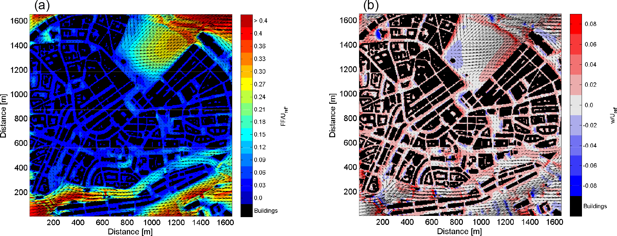
Figure 5Wind field at pedestrian height level in the city center of Hamburg (Germany) showing the normalized wind speed (a) and the vertical wind (b). Black arrows qualitatively show the wind circulation. The simulated domain size is approximately 2000 m×2000 m and the x and y axes are aligned to the west–east and north–south directions, respectively. The simulated mean wind direction is southwest and the atmospheric stratification is neutral. A grid spacing of 5 m in all spatial directions is used. All input data are taken from the digital terrain model, the data of the Germangeo information system ATKIS (Official Topographic–Cartographic Information System), and the 3-D urban model data (LoD2) for building details.
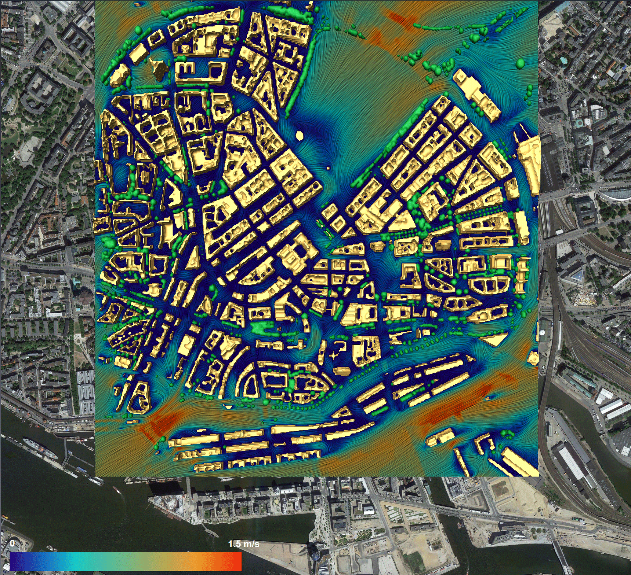
Figure 6Snapshot of the wind speed in the city center of Hamburg (Germany) from a simulation that includes the effect of trees. The simulated domain (2000 m×2000 m) contains about 2800 trees with 130 different species. Buildings and trees are displayed in shades of yellow and green, respectively. The animation setup was kindly provided by Niklas Röber at DKRZ. The copyright for the underlying satellite image is held by GeoBasis-DE/BKG (©2009), Google.
6.2 Wind flow field in a realistic urban domain
MITRAS has been used to simulate the wind flow field in the city center of Hamburg in Germany. The selected domain has a size of 2×2 km2 and represents a typical urban area with many features of urban complexity such as complex building geometries, different street configurations, and diverse surface covers (including water bodies, street pavements, and open spaces). All available building data (shapes, dimensions, locations, etc.), orography heights, and the surface cover characteristics of the domain are utilized to generate the required input data for MITRAS. The meteorological conditions used in this simulation are set so that the wind speed is 3 m s−1 at 200 m above the ground and the wind direction is 230∘, which is a typical wind direction in Hamburg. The results are shown in Fig. 5 in which wind speed and vertical wind are plotted at the pedestrian height (vertical) level. The results describe the effects of buildings on the flow field and show several flow features such as wind speed acceleration in open areas, deceleration within dense building configurations, and updrafts and downdrafts around the buildings. Moreover, the figure shows that buildings alter the wind flow field and, additionally, the orography and surface characteristics modify the wind.

Figure 7Vertical cross section at the center of a high-rise building located in Hamburg (Germany) on 1 February at 13:30 parallel to the wind direction. Colors show the potential temperature of the air surrounding the building and arrows depict the wind circulation for both the reference case (no thermal energy exchange between building façades and environment, a) and the case with full model physics as described in Sect. 4.2 (b). Comparing both cases indicates that the air is slightly heated up by the buildings, especially in the building stagnation and wake regions.
6.3 The effect of urban vegetation on wind field
MITRAS simulations with different parameterizations of urban vegetation (especially trees) were recently performed by Salim et al. (2015) to study the effect of the inclusion of trees when simulating the wind flow in different urban complexities. This study showed a significant effect of trees on the wind field and thus highlights the importance of the explicit representation of urban trees in microscale simulations. A snapshot of an animation created from the simulations performed in this study is shown in Fig. 6 and displays the wind field when the trees are considered in the simulation together with the tree sizes and locations. More details about this study can be found in Salim et al. (2015).
6.4 Thermal effect of buildings
To show the thermal effect of a building on its surroundings, several simulations have been done using MITRAS. The building surface temperature is calculated as described in Sect. 4.2 to simulate a single high-rise building located in an urban area in Hamburg on 1 February at 13:30 (GMT + 2; Gierisch, 2011). Figure 7 shows the thermal effect of such building by comparing the air temperature field with a reference case, in which the thermal energy flux from building façades is neglected.
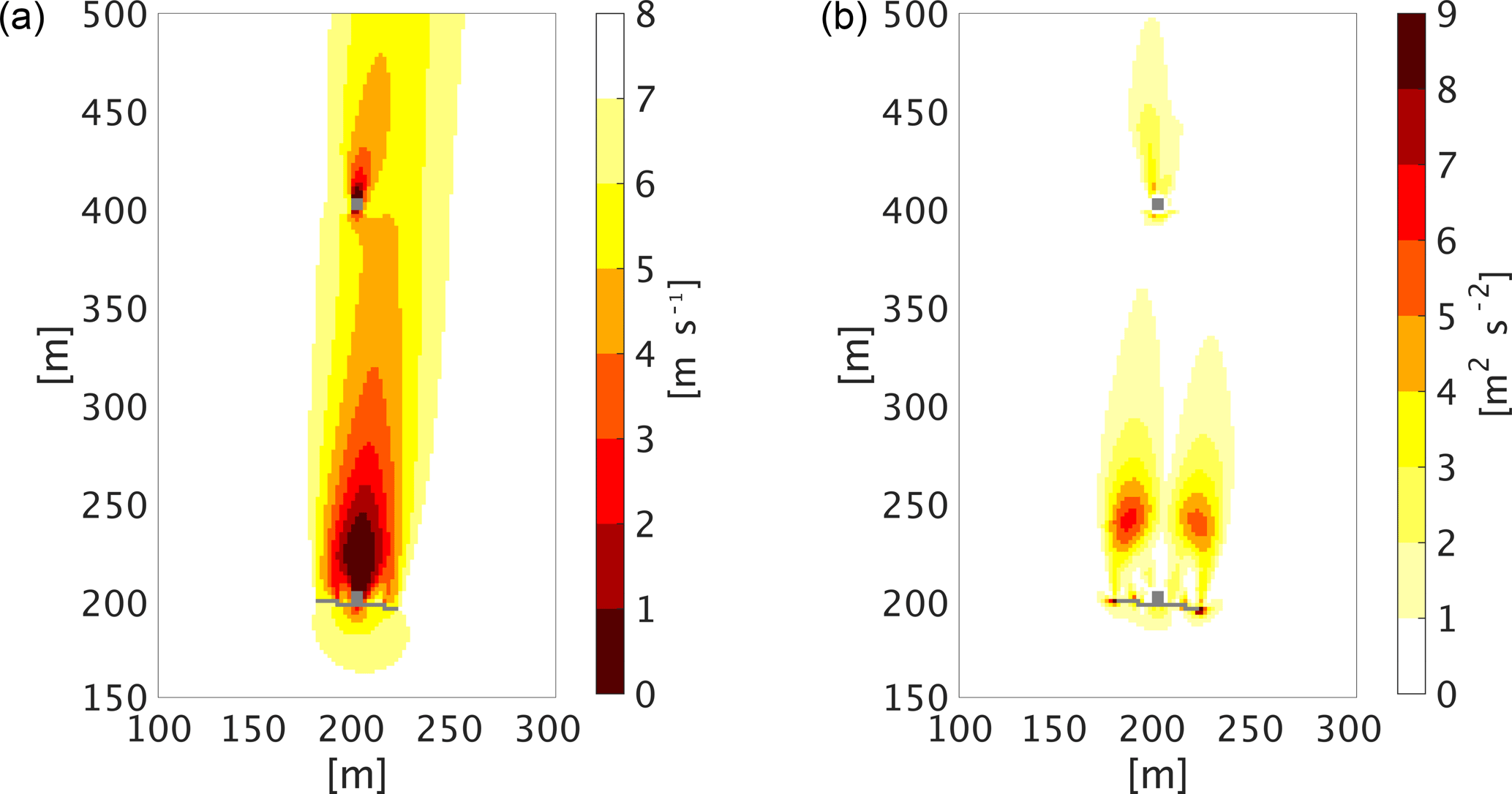
Figure 8Horizontal cross section of the domain at 38 m of height showing (a) the wind speed and (b) the turbulent kinetic energy (right) in the vicinity of a wind turbine (Nibe B) and the tower of another wind turbine (Nibe A, out of service in the simulation). A mean wind flow of 8.5 m s−1 in the south direction was simulated in a neutrally stratified flow. The roughness length is set to 0.014 m and the Coriolis force is considered in the simulation.
6.5 The impact of wind turbines on atmospheric flow
The model MITRAS, with embedded wind turbine parameterizations (see Sect. 4.3), has been used to produce simulation data for model validations (Linde, 2011). The selected case in this study involved the Nibe wind turbines in Nibe, Denmark. This case is selected because there is a meteorological measurement dataset for these wind turbines (Taylor, 1990). Figure 8 gives one example of the model results from this study. Comparisons of model results with the measurements showed a good agreement.
The model theory of the obstacle-resolving microscale meteorological model MITRAS version 2 has been described in this paper. Detailed descriptions of the model equations and their formulations and approximations are presented. The sub-grid-scale turbulence parameterization used in MITRAS is outlined showing the Prandtl–Kolmogorov closure and the 1.5-order E–ε turbulence closure. Also, detailed parameterizations of obstacles such as wind turbines and vegetation (trees) are introduced. The different boundary conditions implemented in MITRAS and the model inputs are also outlined. The model dynamics and numerical framework of MITRAS are established to provide a solid foundation for future model extensions.
Verification experiments of MITRAS version 2 with the simulation of urban areas with explicitly resolved obstacles (including buildings, wind turbines, and trees) will be presented in a separate paper. A recent application of MITRAS version 2 to vegetation effects in urban areas can be found in Salim et al. (2015).
Currently the MITRAS source code is distributed upon request under the terms of a user agreement with the Mesoscale and Microscale Modeling (MeMi) working group at the Meteorological Institute, University of Hamburg (https://www.mi.uni-hamburg.de/memi). A copy of the user agreement is available upon request. Due to current copyright restrictions, users are requested to contact the corresponding authors to obtain access to the code free of charge for research purposes under a collaboration agreement (metras@uni-hamburg.de).
Documentation for the M-SYS model system (Schlünzen et al., 2018a, b), in which MITRAS is included, is available online at https://www.mi.uni-hamburg.de/memi under “Numerical Models”.
The numerical method for calculating the dissipation term in the SGS TKE equation is based on splitting the SGS TKE prognostic equation into two parts. In the first part all processes except dissipation are integrated within a time step Δt to get a preliminary value of TKE, . In the second part TKE at the end of the complete time step is used to integrate the dissipation term.
The dissipation is parameterized according to Eq. (13), which can be simplified as
where C is a constant. Overall, the following equation is solved in the second step.
By integrating Eq. (A3), assuming ρ0, α∗, and l(Ri) to be constant within one time step, the analytic solution for the TKE dissipation is calculated as follows.
A similar solution for the dissipation term in the TKE equation of the SGS model suggested by Deardorff (1980), suitable for large eddy simulation, is presented in Fock (2015).
MS organized the paper and collected the contributions. He also developed the preprocessor GRIMASK and is responsible for the ideas behind it (Sect. 4). He included different vegetation treatments in MITRAS (Sect. 4.4) and provided model results on this (Sect. 6.3) as well as a realistic application (Sect. 6.2). HS coordinated the model development since the beginning and is overall responsible for the model and its documentation. She provided a number of comments on the paper, as did DG, who is responsible for model evaluation (Sect. 6.1) and aspects concerning model quality assurance and code provision. MB contributed the wind turbine development to MITRAS (Sect. 4.3) and corresponding results (Sect. 6.5), and AG implemented the calculation of building surface temperatures (Sect. 4.3) and provided results on this (Sect. 6.4). BF derived the analytic solution for the E−ϵ relation (Eq. 13, Appendix A).
The authors declare that they have no conflict of interest.
This research is supported through the Cluster of Excellence “CliSAP”
(EXC177) and the research project UrbMod funded by the state of Hamburg,
Germany. The authors would like to thank the two anonymous reviewers and
the topical editor David Ham for their helpful and constructive comments and
support during the review process.
Edited by:
David Ham
Reviewed by: two anonymous referees
Arakawa, A. and Vivian, R. L.: Computational Design of the Basic Dynamical Processes of the UCLA General Circulation Model, Method. Comput. Phys., 17, 173–265, 1977.
Briscolini, M. and Santangelo, P.: Development of the Mask Method for Incompressible Unsteady Flows, J. Comput. Phys., 84, 57–75, 1989.
Bruse, M. and Fleer, H.: Simulating Surface–plant–air Interactions inside Urban Environments with a Three Dimensional Numerical Model, Environ. Model. Softwa., 13, 373–84, 1998.
Brutsaert, W.: The Roughness Length for Water Vapor Sensible Heat, and Other Scalars, J. Atmos. Sci., 32, 2028–31, 1975.
Brutsaert, W.: Evaporation into the Atmosphere: Theory, History and Applications, Vol. 1, Springer Science & Business Media, 302 pp., https://doi.org/10.1007/978-94-017-1497-6, 2013.
Clark, T. L.: A Small-Scale Dynamic Model Using a Terrain-Following Coordinate Transformation, J. Comput. Phys., 24, 186–215, 1977.
Deardorff, J. W.: Efficient Prediction of Ground Surface Temperature and Moisture, with Inclusion of a Layer of Vegetation, J. Geophys. Res.-Oceans, 83, 1889–1903, 1978.
Deardorff, J. W.: Stratocumulus-capped mixed layers derived from a three-dimensional model, Bound.-Lay. Meteorol., 18, 495–527, 1980.
Detering, H. W.: Mixing Length and Turbulent Diffusion Coefficient in Atmospheric Simulation models, Thesis, Technische Univ., Hanover, Germany, 1985.
Durran, D. R. and Joseph, B. K.: The Effects of Moisture on Trapped Mountain Lee Waves, J. Atmos. Sci., 39, 2490–2506, 1982.
Dyer, A. J.: A Review of Flux-Profile Relationships, Bound.-Lay. Meteorol., 7, 363–372, 1974.
Eichhorn, J.: Entwicklung und Anwendung einesdDreidimensionalen mikroskaligen Stadtklima-Modells, PhD dissertation, University of Mainz, Mainz, Germany, 1989.
Eichhorn, J. and Kniffka, A.: The Numerical Flow Model MISKAM: State of Development and Evaluation of the Basic Version, Meteorol. Z., 19, 81–90, 2010.
El Kasmi, A. and Christian M.: An Extended K–ε Model for Turbulent Flow through Horizontal-Axis Wind Turbines, J. Wind Eng. Ind. Aerod., 96, 103–22, 2008.
Etling, D.: The Planetary Boundary Layer PBL, in: Landolt-Börnstein – Group V Geophysics, Meteorology – Climatology, Part 1, edited by: Fischer, G., Group V, 4, 151–88, https://doi.org/10.1007/10356990_33, 1987.
Fischereit, J., Schlünzen, K. H., Gierisch, A. M. U., Grawe, D., and Petrik, R.: Modelling tidal influence on sea breezes with models of different complexity, Meteorol. Z., 25, 343–355, https://doi.org/10.1127/metz/2016/0703, 2016.
Fock, B. H.: RANS versus LES Models for Investigations of the Urban Climate, Thesis, University of Hamburg, Hamburg, Germany, available at: http://ediss.sub.uni-hamburg.de/volltexte/2015/7171/pdf/Dissertation.pdf (last access: 27 July 2018), 2015.
Foken, T.: 50 Years of the Monin–Obukhov Similarity Theory, Bound.-Lay. Meteorol., 119, 431–47, 2006.
Franke, J., Sturm, M., and Kalmbach, C.: Validation of OpenFOAM 1.6. X with the German VDI Guideline for Obstacle Resolving Micro-Scale Models, J. Wind Eng. Ind. Aerod., 104, 350–359, 2012.
Früh, B., Becker, P., Deutschländer, T., Hessel, J. D., Kossmann, M., Mieskes, I., Namyslo, J., Roos, M., Sievers, U., Steigerwald, T., and Turau, H.: Estimation of climate-change impacts on the urban heat load using an urban climate model and regional climate projections, J. Appl. Meteorol. Climatol., 50, 167–184, 2011.
Gerz, T., Holzaepfel, F., Darracq, D., de Bruin, A., Elsenaar, A., Speijker, L., Harris, M., Vaughan, M., and Woodfield, A. A.: Aircraft Wake Vortices – a Position Paper, Wakenet position paper, WakeNet – the European Thematic Network on Wake Vortex, 80 pp., 2001.
Gierisch, A.: Mikroskalige Modellierung meteorologischer und anthropogener Einflüsse auf die Wärmeabgabe eines Gebäudes, Master Thesis, University of Hamburg, Hamburg, Germany, available at: https://mi-pub.cen.uni-hamburg.de/fileadmin/files/forschung/techmet/nummod/thesis/diplom_andrea_gierisch.pdf (last access: 17 July 2018), 2011.
Grawe, D., Schlünzen, K. H., and Pascheke, F.: Comparison of Results of an Obstacle Resolving Microscale Model with Wind Tunnel Data, Atmos. Environ., 79, 495–509, 2013.
Grawe, D., Bächlin, W., Brünger, H., Eichhorn, J. Franke, J., Leitl, B., Müller, W., Öttl, D., Salim, M. H., Schlünzen, H., Winkler, C., and Zimmer, M.: An Updated Evaluation Guideline for Prognostic Microscale Wind Field Models, 9th International Conference on Urban Climate, Toulouse, France, 20–24 July, 2015.
Gross, G.: Effects of Different Vegetation on Temperature in an Urban Building Environment. Micro-Scale Numerical Experiments, Meteorol. Z., 21, 399–412, 2012.
Harms, F., Leitl, B., Schatzmann, M., and Patnaik, G.: Validating LES-Based Flow and Dispersion Models, J. Wind Eng. Ind. Aerod., 99, 289–295, 2011.
Kapitza, H. and Eppel, D.: A 3-D Poisson Solver Based on Conjugate Gradients Compared to Standard Iterative Methods and Its Performance on Vector Computers, J. Comput. Phys., 68, 474–484, 1987.
Kato, M. and Launder, B. E.: The Modelling of Turbulent flow around stationary and vibrating square cylinders, 9th Symposium on Turbulent Shear Flows, Kyoto, Japan, 16–18 August, 1993.
Katul, G.: An Investigation of Higher-Order Closure Models for a Forested Canopy, Bound.-Lay. Meteorol., 89, 47–74, 1998.
Lalic, B. and Mihailovic, D. T.: An Empirical Relation Describing Leaf-Area Density inside the Forest for Environmental Modeling, J. Appl. Meteorol., 43, 641–45, 2004.
Lilly, D. K.: On the Numerical Simulation of Buoyant Convection, Tellus, 14, 148–172, 1962.
Linde, M.: Modellierung des Einflusses von Windkraftanlagen auf das umgebende Windfeld, Master Thesis, University of Hamburg, Hamburg, Germany, available at: https://mi-pub.cen.uni-hamburg.de/fileadmin/files/forschung/techmet/nummod/thesis/Diplomarbeit_M_Linde.pdf (last access: 17 July 2018), 2011.
Liu, J., Chen, J. M., Black, T. A., and Novak, M. D.: E-ε Modelling of Turbulent Air Flow Downwind of a Model Forest Edge, Bound.-Lay. Meteorol., 77, 21–44, 1996.
López, S. D.: Numerische Modellierung Turbulenter Umströmungen von Gebäuden, Berichte zur Polar-und Meeresforschung (Reports on Polar and Marine Research) 418, 93 pp., 2002.
López, S. D., Lupkes, C., and Schlünzen, K. H.: The Effect of Different K-Closures on the Results of a Micro-Scale Model for the Flow in the Obstacle Layer, Meteorol. Z., 14, 839–848, 2005.
Maronga, B., Gryschka, M., Heinze, R., Hoffmann, F., Kanani-Sühring, F., Keck, M., Ketelsen, K., Letzel, M. O., Sühring, M., and Raasch, S.: The Parallelized Large-Eddy Simulation Model (PALM) version 4.0 for atmospheric and oceanic flows: model formulation, recent developments, and future perspectives, Geosci. Model Dev., 8, 2515–2551, https://doi.org/10.5194/gmd-8-2515-2015, 2015.
Meng, C.: The integrated urban land model, J. Adv. Model. Earth Sy., 7, 759–773, 2015.
Mikkelsen, R.: Actuator Disc Methods Applied to Wind Turbines, PhD Thesis, Technical University of Denmark, Copenhagen, Denmark, available at: http://orbit.dtu.dk/fedora/objects/orbit:85749/datastreams/file_5452244/content (last access: 17 July 2018), 2003.
Mittal, R. and Iaccarino, G.: Immersed Boundary Methods, Annu. Rev. Fluid Mech., 37, 239–61, 2005.
Molly, J.-P.: Windenergie in Theorie und Praxis: Grundlagen und Einsatz, Müller, karlsruhe, Germany, 138 pp., 1978.
Monin, A. S. and Obukhov, A.: Basic Laws of Turbulent Mixing in the Surface Layer of the Atmosphere, Contrib. Geophys. Inst. Acad. Sci., USSR 151, 163–187, 1954.
Müller, N., Kuttler, W., and Barlag, A.: Counteracting Urban Climate Change: Adaptation Measures and Their Effect on Thermal Comfort, Theor. Appl. Climatol., 115, 243–257, 2014.
Murakami, S., Ooka, R., Mochida, A., Yoshida, S., and Kim, S.: CFD Analysis of Wind Climate from Human Scale to Urban Scale, J. Wind Eng. Ind. Aerod., 81, 57–81, 1999.
Pielke, R. A.: Mesoscale Meteorological Modeling, Academic press, 676 pp., 2002.
Roache, P. J.: Scaling of High-Reynolds-Number Weakly Separated Channel Flows, in: Numerical and Physical Aspects of Aerodynamic Flows, Springer, 87–98, https://doi.org/10.1007/978-3-662-12610-3_6, 1982.
Röber, N., Salim, M. H., Gierisch, A., Böttinger, M., and Schlünzen, K. H.: Visualization of Urban Micro-Climate Simulations, The Eurographics Association, 53–57, 2013.
Salim, M. H., Schlünzen, K. H., and Grawe, D.: Including Trees in the Numerical Simulations of the Wind Flow in Urban Areas: Should We Care?, J. Wind Eng. Ind. Aerod., 144, 84–95, 2015.
Salim, M. H., Linde, M., Gierisch, A., and Schlünzen, K. H.: Some Recent Extensions and Applications of the Micro-Scale Model MITRAS, presented at the 10th European Conference on Applications of Meteorology (ECAM)/11th EMS Annual Meeting, Berlin, Germany, 12–16 September, 2011.
Schafer, K., Emeis, S., Hoffmann, H., Jahn, C., Muller, W., Heits, B., Haase, D., Drunkenmolle, W. D., Bachlin, W., Schlünzen, K., and Leitl, B.: Field Measurements within a Quarter of a City Including a Street Canyon to Produce a Validation Data Set, Int. J. Environ. Pollut., 25, 201–216, 2005.
Schatzmann, M., Bächlin, W., Emeis, S., Kühlwein, J., Leitl, B., Müller, W. J., Schäfer, K., and Schlünzen, H.: Development and validation of tools for the implementation of european air quality policy in Germany (Project VALIUM), Atmos. Chem. Phys., 6, 3077–3083, https://doi.org/10.5194/acp-6-3077-2006, 2006.
Schlünzen, K. H.: Numerical Studies on the Inland Penetration of Sea Breeze Fronts at a Coastline with Tidally Flooded Mudflats, Contr. Atmos. Phys., 63, 243–256, 1990.
Schlünzen, K. H., Hinneburg, D., Knoth, O., Lambrecht, M., Leitl, B., Lopez, S., Lüpkes, C., Panskus, H., Renner, E., Schatzmann, M., and Schoenemeyer, T.: Flow and Transport in the Obstacle Layer: First Results of the Micro-Scale Model MITRAS, J. Atmos. Chem., 44, 113–130, 2003.
Schlünzen, K. H., Boettcher, M., Fock, B. H., Gierisch A., Grawe D., and Salim, M.: Technical Documentation of the Multiscale Model System M-SYS (METRAS, MITRAS, MECTM, MICTM, MESIM) Meteorologisches Institut, Universität Hamburg, MeMi Technical Report 3, 130 pp., 2018a.
Schlünzen, K. H., Boettcher, M., Fock, B. H., Gierisch, A., Grawe, D., and Salim, M.: Scientific Documentation of the Multicscale Model System M-SYS (METRAS, MITRAS, MECTM, MICTM, MESIM) Meteorologisches Institut, Universität Hamburg, MeMi Technical Report 4, 147 pp., 2018b.
Schlüter, I.: Simulation des Transports biogener Emissionen in und über einem Waldbestand mit einem mikroskaligen Modellsystem, PhD Thesis, University of Hamburg, Hamburg, Germany, available at: https://d-nb.info/98143021X/34 (last access: 17 July 2018), 2006.
Smagorinsky, J.: General Circulation Experiments with The Primitive Equations: I. The Basic Experiment, Mon. Weather Rev., 91, 99–164, 1963.
Taylor, G. J.: Wake measurements on the Nibe wind turbines in Denmark, Contractor report ETSU WN 5020, National Power – Technology and Environment Center, 1990.
Tiedtke, M. and Geleyn, J. F.: The DWD General Circulation Model – Description of Its Main Features, Beitr. Phys. Atmos., 48, 255–277, 1975.
Trukenmuller, A., Grawe, G., and Schlünzen, K. H.: A Model System for the Assessment of Ambient Air Quality Conforming to EC Directives, Meteorol. Z., 13, 387–394, 2004.
Van der Vorst, H. A.: Bi-CGSTAB: A Fast and Smoothly Converging Variant of Bi-CG for the Solution of Nonsymmetric Linear Systems, SIAM J. Scientific and Stat. Comp., 13, 631–44, 1992.
VDI: Environmental Meteorology – Prognostic Microscale Wind Field Models – Evaluation for Flow Around Buildings and Obstacles, Technical Report, VDI Guideline 3783, Part 9, Commission on Air Pollution Prevention of VDI and DIN, 2005.
VDI: Environmental Meteorology, Prognostic Microscale Wind Field Models, Evaluation for Flow around Buildings and Obstacles, VDI-Standard: VDI 3783, Blatt 9, available at: http://www.vdi.eu/guidelines/vdi_3783_blatt_9-umweltmeteorologie_prognostische_mikroskalige_windfeldmodelle_evaluierung_fuer_gebaeude_/ (last access: 27 July 2018), 2015.
Wilson, J. D.: A Second-Order Closure Model for Flow through Vegetation, Bound.-Lay. Meteorol., 42, 371–392, 1988.