High-performance software framework for the calculation of satellite-to-satellite data matchups (MMS version 1.2)

We present a multisensor matchup system (MMS) that allows systematic detection of satellite-based sensor-to-sensor matchups and the extraction of local subsets of satellite data around matchup locations. The software system implements a generic matchup-detection approach and is currently being used for validation and sensor harmonization purposes. An overview of the flexible and highly configurable software architecture and the target processing environments is given. We discuss improvements implemented with respect to heritage systems, and present some performance comparisons. A detailed description of the intersection algorithm is given, which allows a fast matchup detection in geometry and time.

1 Introduction

There is increasing exploitation of Earth observation (i.e., satellite remote sensing) data for a range of scientific and societal applications, in relation to environmental monitoring including climate science (e.g., Hollmann et al., 2013). Often, long (multi-decadal) data records are required for such applications, so that observed changes can be put in the context of a time series of earlier variability, for example to determine how common a particular observation is. Since satellite missions typically last 5 years, such long data records need to be constructed from a series of data records from similar but not identical sensors. The differences among members of such sensor series consist of factors such as detailed spectral responses (i.e., slightly different sensitivities to Earth radiation at different wavelengths), differences in calibration procedures and performance in flight, the effects over time through each mission of degradation of the sensors, and so on. Such differences can cause significant discontinuity in the derived records of environmental variables among different sensors, and steps need to be taken to minimize such artifacts, essentially to maximize the signal for real natural variability compared to sensor-difference effects. A key tool for harmonizing satellite-derived data records across multiple sensors is to compare, to as close an approximation as possible, the radiances observed by sensors when viewing the same environmental scene simultaneously. Such paired observations are referred to as matchups and are critical to exploit for multisensor data records. This paper addresses progress on the important practical step of creating datasets of matchups to use for harmonizing or bias-correcting across sensors to create consistent, multi-decadal data records.

The detection of satellite data matchups is a numerically intensive process that incorporates geographic searches in large satellite datasets, which may be on the order of 100 TB in size. A highly performing search and data extraction system has to be operated in a parallel processing environment to achieve manageable processing times for this task. Despite the importance of being able to analyze long time series of matchup data, surprisingly few general concepts are published to detect and extract the data. Some publications use a relatively small number of satellite intersections that have been detected manually (e.g., Illingworth et al., 2009), whereas other teams develop custom solutions for restricted pairs of sensors (e.g., Bali et al., 2015). A generic concept for matchup generation has been implemented for the project FELYX (Taberner et al., 2013). Our review of this option concluded that the specifications did not match the criteria for flexible mass production and analysis of whole mission datasets.

For the European Space Agency Climate Change Initiative project for Sea Surface Temperature (SST CCI), a first system to identify and generate sensor–sensor matchups has been developed in an early phase of the project (Boettcher et al., 2012). This system, initially targeted to operate on a single dataset, has been used and extended during the project lifetime (the past 6 years). Increasing input dataset sizes, stricter requirements on matchup conditions, and the necessity to operate on small matchup time differences led to the decision to create a completely new software that implements all the lessons learned during operations of the earlier software. The current system is operated on the Climate and Environmental Monitoring from Space (CEMS) facility at the Centre for Environmental Data Analysis (CEDA)¹ . The same architecture is also being further developed within the framework of the European Union project “Fidelity and uncertainty in climate data records from Earth Observations” (FIDUCEO).

The initial system exhibited some performance bottlenecks, predominantly caused by the way a database was used, too many read accesses to satellite data products, and a fixed processing time interval. Especially the use of the database as a storage location for satellite acquisition metadata and matchup candidate locations (i.e., read and write access to the same database) prevented a significant parallelization to improve the overall performance. Design goals for the new system architecture have been defined as follows.

• Use the database only for storage of satellite metadata, distribute numerically expensive geometric calculations to parallel nodes, and keep the matchup candidate data locally.

• Implement a system that allows reading of the satellite data products late in the matchup detection process. The software shall detect matchup candidate pairs reliably before actually accessing the file system – reducing several hundred possible candidate products to a small number of consolidated candidates.

• Design the system as an extensible frame with a large number of plug-in points.

• Facilitate integration of new sensors.

• Implement a scalable system that can run on a notebook as well as allow a high parallelization on a dedicated processing environment, avoiding single points of access.

Following these design goals we have implemented a high-performance matchup system that has already generated various long-term sensor matchup datasets, ranging from 1979 to 2016, covering combinations of seven visible and microwave sensors from 23 different satellite platforms in processing levels L1 and L2, both as full orbit acquisitions and granules.

The MMS consists of three major components:

• a database server for the storage of satellite data metadata records,

• an “IngestionTool” to extract the metadata from the satellite acquisitions and store them in the database, and

• a “MatchupTool” that performs the matchup processing and writing of the resulting data.

The interaction of these components implements the functionality described in the following sections.

2 Definition

In the context of the SST CCI and FIDUCEO projects, we define a satellite data matchup as a coinciding measurement of the same location on Earth at almost the same time using different spaceborne instruments. The location criterion is defined as the geodesic distance in kilometers among pixel center locations; the time constraint is defined as pixel acquisition time difference.

In most use cases there are additional criteria on top of this raw matchup definition, which include for example cloud-free conditions, constraints on the viewing angles, water pixel constraint, and many more; we summarize these conditions as screening criteria (see Sect. 6).

The result of a matchup-processing run is stored as a multisensor matchup dataset (MMD, Sect. 7), which includes all data required to analyze the matchups without the need to access the original satellite input datasets. These MMD files include satellite data extracts covering a symmetrical window of n by m pixels around the matchup point, copying all variables of the input data as a geometrical subset of the target file.

3 Matchup processing

Based on the intention to assemble a generic matchup generation system, we have identified several common steps. During the analysis, we also identified the steps/concepts that require sensor- or domain-specific handling; all of these have been encapsulated as abstractions that hide sensor- or domain-specific implementations. Our design incorporates a database containing satellite acquisition metadata, which has to be filled as a first step:

1. ingest satellite metadata into database.

   Any matchup generation process starts with a database query:

2. request sensor metadata for time interval and sensor combination to process,

3. perform matchup candidates preselection (Sect. 4),

4. perform matchup candidates fine selection (Sect. 5),

5. run condition and screening processes (Sect. 6),

6. assemble subset data and write MMD (Sect. 7).

These steps are implemented using two distinct programs, an IngestionTool (performing step 1) and a MatchupTool (performing steps 2 to 6).

4 Metadata and candidates preselection

For each satellite data product accessible to the MMS system a corresponding metadata record is stored in the database. The metadata record contains information about the data file location, the sensor, the acquisition time, the bounding geometry of the acquisition, the orbit nadir trajectory, an ascending or descending node flag, and the data processor version. This data record has been designed to optimize database storage volume (and hence access performance) while keeping sufficient information to operate the matchup system.

4.1 Metadata extraction

The satellite metadata stored in the database has been constructed in a way that allows the detection of overlapping regions possibly containing matchups without the need to open the associated satellite data products. The detection is a two-step process that consists of the detection of a geometric intersection followed by a calculation of the acquisition times of both sensors for the common area. If the acquisition times match, taking into account the maximal pixel time difference allowed, a set of possible matchup pairs has been detected.

The geometry metadata for each satellite product is constructed using the approach sketched in Fig. 1. Two entities are generated by regularly sampling longitude–latitude pairs from the geo-location data rasters: a bounding polygon and a time axis line string following the nadir track of the satellite. The bounding polygon is constructed by stepping around the borders of the rasters, in a counter-clockwise direction; the time axis is constructed by sampling in flight direction at the center of the swath acquisition – ignoring the 1 pixel offset occurring in products with an even number of pixels per line. In case of self overlaps (which happen often for the Advanced Very-High-Resolution Radiometer (AVHRR) data) the geometries are split into two segments to ensure valid geometry objects.

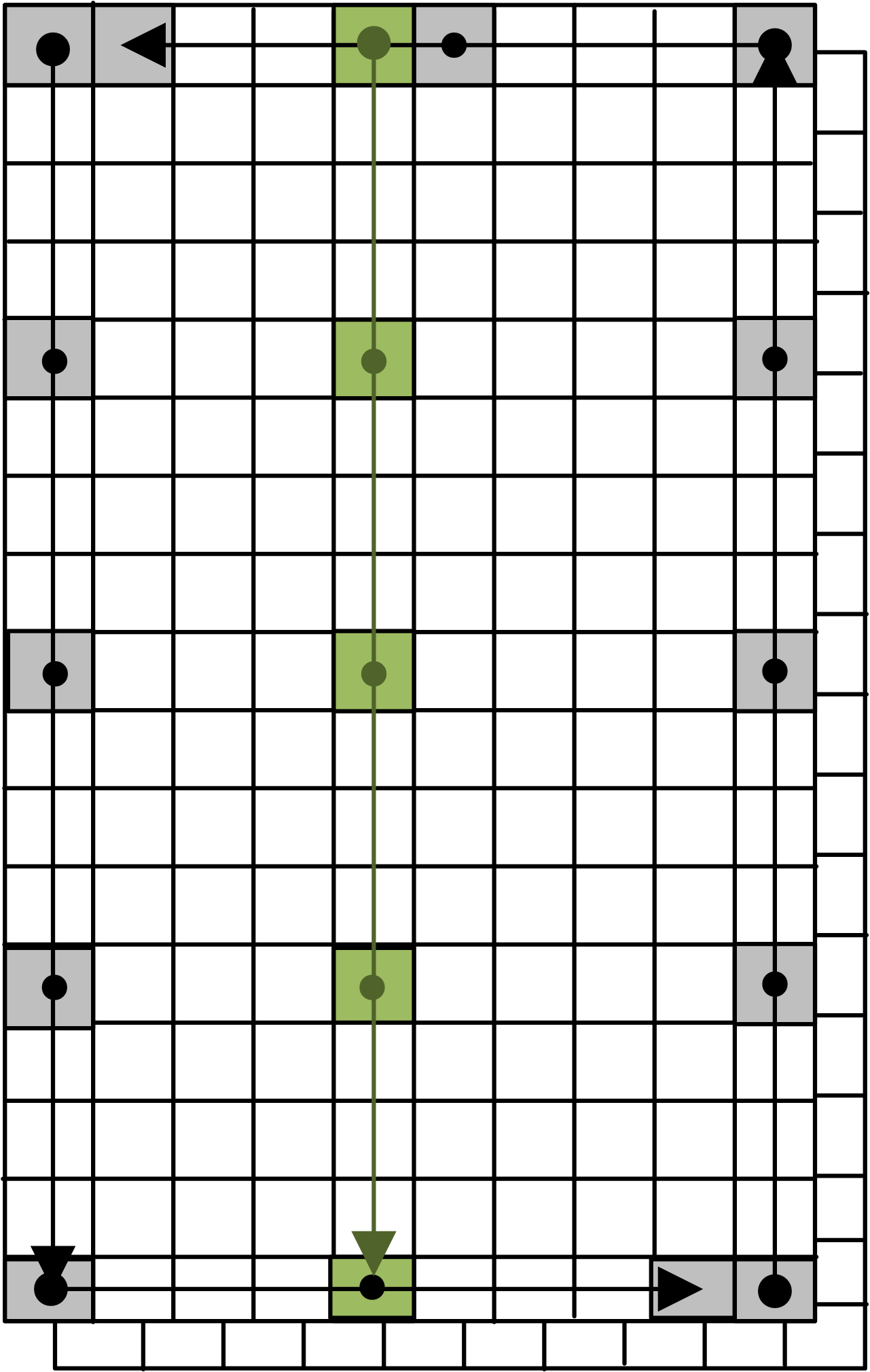
Figure 1 Construction of the satellite product boundary polygon (black) and time axis line string (green). The rasters are the longitude and latitude data arrays; acquisition time increases from the top downwards.

4.2 Intersection detection

A geometric intersection between two satellite acquisitions can simply be calculated by performing an intersection of the associated satellite data bounding geometries. The calculation of the timing intersection is not as simple as this; the acquisition times of the data are stored with the satellite data, in most cases either per pixel or per scan line. This means that the timing information is stored in the swath coordinate system (x∕y acquisition raster), whereas to be useful for geometric intersection calculation, the timing data need to be in a geographic (longitude–latitude) coordinate system. Mathematical transformations

$$\begin{array}{}\text{(1)}& f\left(x,y\right)=\left(\mathit{\varphi },\mathit{\lambda }\right)\text{and}g\left(\mathit{\varphi },\mathit{\lambda }\right)=\left(xy\right)\end{array}$$

between the coordinate systems can be calculated using polynomial approximations, but these operations require access to the full longitude and latitude data raster. To avoid these time-consuming reading and approximation operations, the MMS implements a different approach based on two assumptions with respect to polar orbiting satellite data.

1. The satellite moves locally with constant velocity on a continuing orbit path.

2. Acquisitions per time instant are located on an axis normal to the nadir point path, which is true for push-broom-type instruments and almost true for scanning instrument types for which the instrument field of view tracks along the nadir plane.

Consequently, a time axis geometry is constructed using the approach described above, i.e., we create a line-string geometry at the nadir pixel by sampling the location data at regular intervals, e.g., every 20 scan lines (see Fig. 1). When associating the sensing start and stop times of the acquisition with the start and end points of the line string, we can approximate the acquisition time of every geo-location on the time axis by taking into account the line length along the axis:

$$\begin{array}{}\text{(2)}& t_{\text{point}}=\left(t_{\text{stop}}-t_{\text{start}}\right){\displaystyle \frac{{\mathrm{\Delta }}_{\text{point-start}}}{{\mathrm{\Delta }}_{\text{stop-start}}}},\end{array}$$

where Δ denotes the length along the line string, which can be calculated using well-known algorithms (e.g., Goodwin, 1910). Based on assumption (2) we can also associate time information with any point within the swath geometry by applying a normal projection along a great circle of the point onto the time axis. This approach allows the calculation of the overflight times of any geometric intersections between two polar orbiting sensors. For the implementation of the geodesic calculations, we rely on the Google S2 library that allows fast geometric calculations on the surface of a three-dimensional spheroid; please also refer to Pandey et al. (2016).

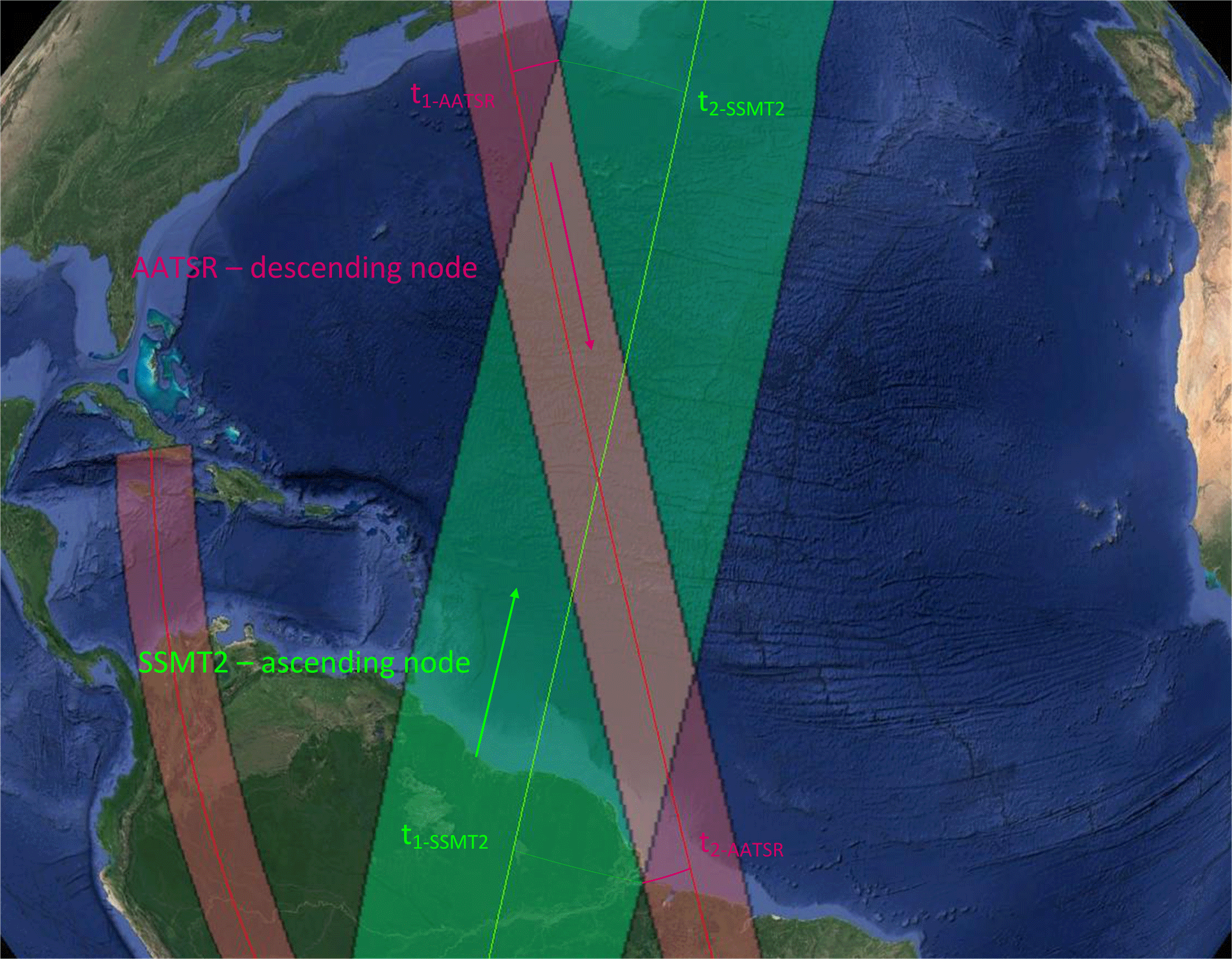
Figure 2 Intersection between Advanced Along-Track Scanning Radiometer (AATSR) and Special Sensor Microwave Water Vapor Profiler (SSM/T-2). AATSR on a descending node; SSM/T-2 on an ascending node. The projection of the intersection geometry extreme locations onto the time axes of both sensors (on the center of the swath) allows the detection of the overflight time. If the time intervals t_1-AATSR–t_2-AATSR and t_1-SSMT2–t_2-SSMT2 are within the configured maximal time delta, possible matchups can be found inside the intersection geometry.

4.3 Time estimation errors

The estimation errors introduced by this approach vary between some milliseconds and up to 17 s for certain AVHRR data. The wide range of errors varies among sensor types and is generally becoming larger for instruments generating wider swath data. However, in the context of natural variability in most environmental parameters at the spatial scales of observation from space, O(10 s) is a relative small error.

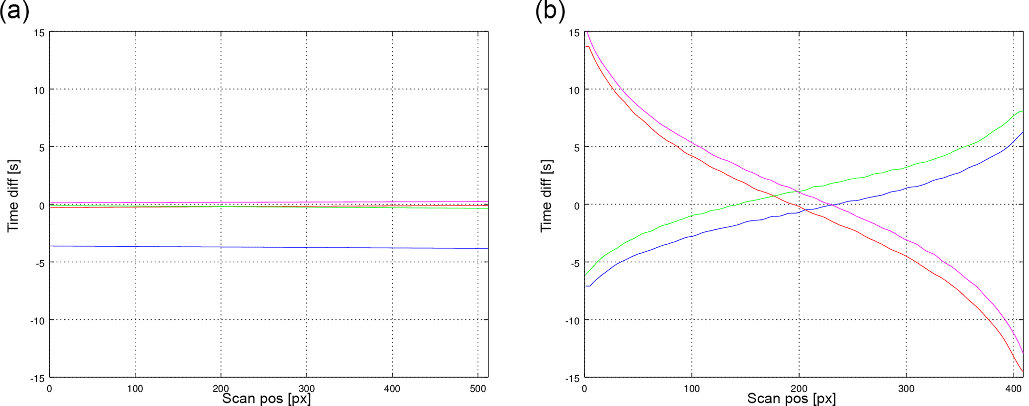
Figure 3 Time error per scan line for AATSR (a) and AVHRR (b). Plotted is the difference between the real and the estimated acquisition time per pixel for the beginning (red), middle (blue and green), and end (magenta) of a full orbit acquisition.

The error distribution per scan line varies from almost constant (AATSR) to a quasi-cubic distribution function (AVHRR). The relatively high estimation precision for AATSR is due to the small swath of 512 km, whereas for the AVHRR case with a swath width of 2892 km the effects of interpolation errors become visible. The larger error line in the AATSR case (blue line in Fig. 3) is generated by the ellipsoid effects; see below.

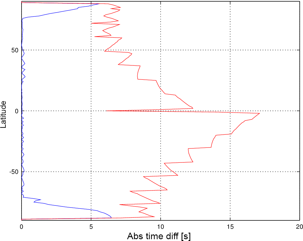
Figure 4 Plot of absolute value of acquisition time estimation error versus latitude for SSM/T-2, minimum value (blue), and maximum value (red).

The estimation errors mainly originate from two effects, both of which can be identified when plotting the estimation error versus latitude (see Fig. 4). In this graph, the blue line displays the minimal estimation error whereas the red line shows the maximal error. It can be seen that a good sensing time projection leads to a difference in the range of milliseconds. The effects of projection are predominantly visible when inspecting the maximum error value plot in red. The sawtooth-like structure is created by the interpolation error that occurs due to the spatial sampling of the time axis. The minima of the sawtooth are located on sampling nodes of the time axis, where no interpolation is required; the maxima are located in the middle between two points using a maximal interpolation length. This error can be minimized by using a smaller interpolation interval, although it has to be balanced with the data storage volumes.

On top of the sawtooth is a constant maximal error that slowly increases from the poles to the Equator. This effect is caused by the underlying assumption that the Earth is a sphere. The deviation of the ellipsoid from a perfect sphere rises to a maximum at the Equator when embedding the sphere into the true Earth form (almost an ellipsoid) so that both geometric forms touch at the poles. The sharp dip at the Equator cannot be explained at the moment and needs further investigation.

In the context of matchup candidate preselection we can easily compensate for these timing errors by adding a sensor-dependent grace interval (i.e., time tolerance) on top of the configured matchup maximum time difference, set by scientific requirements on the matchups according to the purpose of the MMD. Thus, we ensure that we do not reject possible matchup candidate pairs due to interpolation errors.

4.4 Performance comparison

The following table demonstrates the performance gains obtained by the improved preselection algorithm. The time axis approach is described in Sect. 4.1; the full access algorithm implements the standard approach to open each file and read geo-location and timing information to determine the overflight times for the matchup preselection.

Table 1 Performance comparison of the preselection algorithms for some project use cases^∗. Acronyms in this table are ATSR – Along-Track Scanning Radiometer; E2 – ERS2 satellite platform; AVHRR – Advanced Very-High-Resolution Radiometer; Nxx – NOAA xx satellite platform; HIRS – High-resolution Infrared Radiation Sounder; MA – MetOp-A satellite platform; AMSUB – Advanced Microwave Sounding Unit B; SSM/T-2 – Special Sensor Microwave/Temperature-2; F15 – DMSP – F15 satellite platform; AMSRE – Advanced Microwave Scanning Radiometer – Earth Observing System; AQ – Aqua satellite platform; AATSR – Advanced Along-Track Scanning Radiometer; EN – Envisat satellite platform.

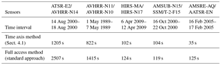
^∗ Tests have been performed on a standard desktop PC: Intel Core i7-5820K, 16 GB RAM, 256 GB SSD for the operating system, 3 TB SATA HD for satellite data, Linux Kubuntu 14.04 64 bit, MongoDB server v3.2.1, Oracle JDK 1.8_45. All tests have been executed three times; the times in the table are the averaged execution times. MMD writing times have been excluded from these measurements.

As demonstrated by the examples in Table 1, the performance gained varies largely between approx. 20 percent up to approximately 350 percent, depending on the input data. Generally, we can conclude here that the performance improvement is small when processing small input data files, e.g., AMSU-B or HIRS, in which the data volumes are in the range of 5 MB and the acquisition raster is small (e.g., 946 × 90 pixels for HIRS). In these cases, the time for loading the geo-location and time datasets is comparably small. The situation changes significantly when processing satellite data with larger volumes, as for example AATSR (ca. 40 000 × 512 pixels, ca. 800 MB), in which performance improvements up to a factor of 2 to 3 can be observed.

Another set of parameters that influences the performance is the duration of the satellite acquisition and the maximal pixel time difference allowed. When the time difference is small compared to the acquisition duration of a product, for example 5 min pixel time difference using AVHRR data with an orbit acquisition time of approximately 1:44 h, there are many geometric intersections within the acquisition time interval of both orbit files. Most of these intersecting geometric areas will be discarded because the common overflight times differ by more than the allowed 5 min time interval. This decision can be made without access to the datasets using the time axis approach, thus avoiding opening a large number of product pairs that are discarded later.

5 Matchup detection

The fine matchup detection process is operating on the reduced set of preselected matchup candidate pairs. This stage of the processing aims to detect all pairs of pixels that comply with the raw matchup conditions as defined in Sect. 2, i.e., time and location condition. The numerically expensive calculations are executed on the consolidated list of candidates, iterating over all pairs of files that have been identified in the preselection stage.

A first step opens both satellite data files, reads the geo-location information, and constructs a geo-coding approximation that implements the mapping between the (ϕ, λ) and (x∕y) coordinate systems as described by Eq. (1). In addition, a TimeCoding object, which maps the sensor specific internal time information to the MMS system reference time (UTC seconds since 1970), is constructed for each of the data files.

For the primary or reference sensor, all pixels contained in the intersection geometry are collected into a list and the closest matching (in a geodesic sense) pixel location in the associated sensor data is calculated². This operation is schematically sketched in Fig. 5.

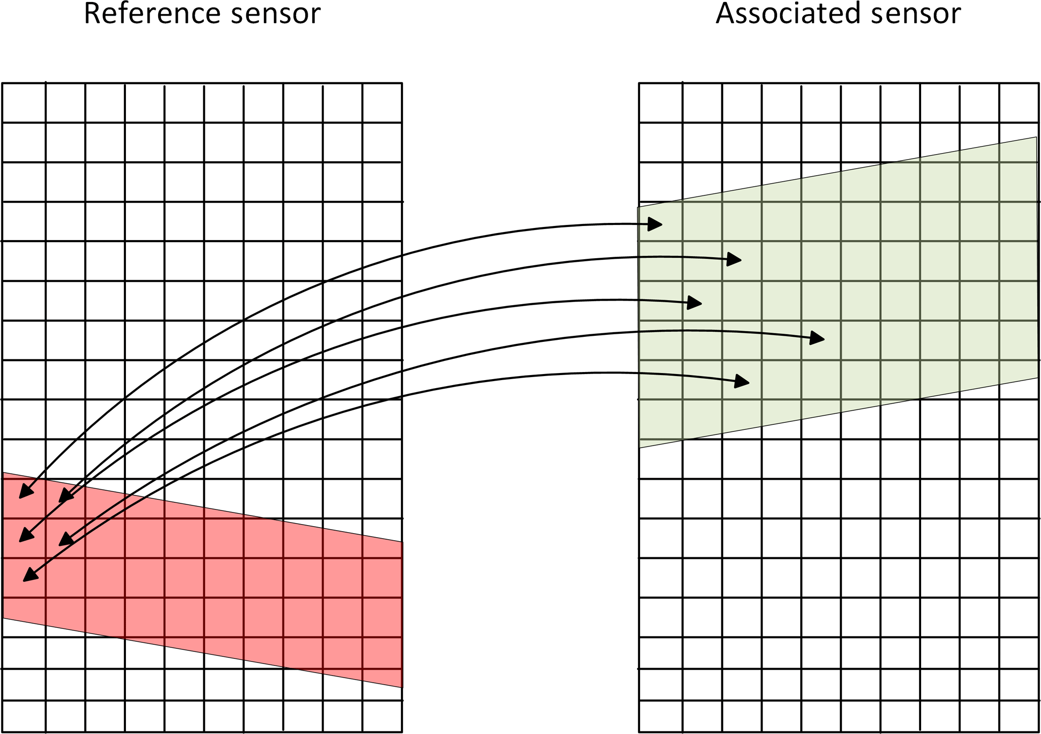
Figure 5 Fine matchup detection, all pixels contained in the intersection geometry of the reference sensor (red) are associated with the closest pixel in the associated sensor data contained in the intersection geometry (green). Both intersection geometries cover the same area in the geographic coordinate system.

Based on these pairs of locations, the acquisition times for both sensors are calculated for each matchup. This list of pixel pairs is immediately scanned for acquisition time difference and spherical distance of pixel centers; all pairs not conforming to the processing parameters (i.e., maximal time difference allowed and maximal pixel center distance) are rejected at this stage. For the pair of satellite acquisitions being processed, the remaining list contains the following values:

• matchup geo-location (long–lat) for both sensors,

• pixel raster position (x∕y) for both sensors,

• acquisition time in UTC seconds since epoch for both sensors.

This list serves as the basis for further processing.

6 Matchup conditions and screenings

The result sets generated up to this processing step contain verified matchup locations conforming to the basic search criteria of acquisition time constraint and relative local neighborhood based on the sensor geo-coding calculations. These can easily contain many tens of thousands of results per intersecting acquisition geometries. In most cases, this list needs to be narrowed down to a smaller subset that conforms to a set of constraints given by the research context. These constraints can be, for example, constraints in the viewing geometries, atmospheric conditions, ground conditions, spatial subsets, instrument conditions, and many more.

The MMS implements a two-step processing stage to perform this narrowing-down procedure, using a very fast first stage, the so-called conditions, and a slower second stage, the screenings. During the second stage, the numerically more intensive screenings operate only on a significantly reduced number of possible matchups that already conform to the conditions, increasing the performance of the overall processing.

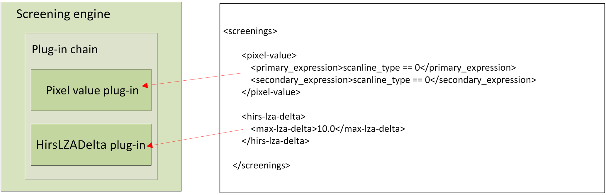
As we expected these processes to vary a lot between the projects and the scientific requirements, we have implemented both processing stages using a general engine–plug-in approach. Each engine operates a chain of plug-ins that are loaded dynamically based on the configuration file, using the Java SPI mechanism (Seacord et al., 2002).

Each plug-in implements a narrow interface and is identified by its unique name. The configuration of the engine is a structured XML document, containing subsections for each plug-in; the order of the subsections defines the order of processing. Plug-in configuration tags allow the identification of the plug-ins, all sub-configurations are passed to the plug-ins to parse so that the engine is completely decoupled from the plug-in module configurations (see Fig. 6).

Figure 6 Screening engine with plug-ins and configuration snippet.

6.1 Conditions

Condition plug-ins operate on the core matchup information solely, i.e., longitude–latitude, product raster x∕y positions, and acquisition times. These entities are kept in memory during processing; thus any condition plug-in executes very fast and is not slowed down by disk access times, for example. Although an extremely reduced parameter set is available, a number of useful condition processes have been implemented, e.g.,

• BorderDistance (reject matchups in which the matchup raster x∕y position is too close to a swath border),

• OverlapRemove (reject pixels in which subset windows overlap).

6.2 Screenings

In contrast, screening plug-ins are also given access to the satellite products associated with the matchups so that any variable from both input files can be used for a screening algorithm. At this stage, it might also be possible to access auxiliary datasets, although this has not been requested yet. A number of sensor-specific and generic algorithms are available; the following list just covers some examples:

• Angular. Performs screening on viewing geometry constraints (e.g., maximal viewing zenith angle (VZA), maximal VZA difference).

• BuehlerCloud. Performs cloud screening for microwave sensors based on Buehler et al. (2007).

• PixelValue. Performs screening that allows the evaluation of mathematical expressions on matchup pixels (e.g., reflec_nadir_0870 > 7.5 & reflec_fward_0670 > 4.3). This plug-in is very generic; it also allows one to define complex flag combinations to be evaluated.

7 Matchup files

The results of the matchup detection and screening processes are finally stored in multisensor matchup datasets (MMDs) using either NetCDF3 or NetCDF4 format. The design of these files shall enable scientists to work with the matchup data without the need to access the original input data files. To allow for this, we copy all input data variables that are contained in a symmetrical n by m pixel window around each matchup to the MMD (the sizes are configurable per sensor). To reflect the calibration purpose of the software, we always copy the data in the original input format, without any modifications or scaling applied. All variable attributes are also copied to the MMD.

For each sensor input variable, the final MMD contains a three-dimensional dataset in which the x and y dimensions are the extensions of the extraction window and the z dimension is the matchup index, i.e., a linear index that counts from 0 to the number of matchups (minus one) that have been detected for the time interval processed. Thus, each z layer in an MMD file contains all data associated with a single sensor–sensor matchup. For sensors that originally contain three-dimensional input data (e.g., HIRS radiance variable), we split the data into separate two-dimensional channel variables. This approach ensures that every ($x/y/z$)-tuple for each variable of each sensor belongs to the same location and time.

In addition to the input data we also store the raw matchup information, namely original raster x and y positions, the unified acquisition time in UTC seconds since epoch and for each z layer the names of the input data files. This ensures that the MMD content is completely traceable and every matchup pair refers to its data origin. One MMD file for each processing interval (e.g., 1 week) is generated on a parallel processing environment.

8 Further work

In addition to the sensors currently supported (AMSR-E, AMSU-B, (A)ATSR, AVHRR, HIRS, MHS, SSM/T2), there are already extensions scheduled to support AIRS, AMSR-2, IASI, MVIRI, and SEVIRI. For the geostationary sensors (MVIRI and SEVIRI) a different preselection approach will be taken. The acquisition time per scene and slot is relatively short and the area covered can be considered constant. In this case, it is expected that the time information alone yields an appropriate preselection criterion.

At the time of writing this text, a first development version of the MMS is also capable of performing satellite and in situ data matchup processing. This first engineering version can operate on SST data collected for the SST CCI project; further extensions scheduled will cover AERONET data and GRUAN radiosonde measurements.

9 Summary and conclusion

We have demonstrated and implemented a general matchup processing system using a novel and fast intersection detection algorithm for polar-orbiting satellite-based sensor overlaps. The time axis approach for acquisition time detection and the use of a novel library for spherical calculations allow performance gains of up to a factor of 3.5 compared to a conservative implementation. We introduced a two-step screening system that is highly configurable to adapt the matchup process to several scientific requirements. The software is designed to be operated on a parallel cluster environment; tests with up to 200 nodes have been executed successfully.

This paper concentrated on the algorithmic facets of the software system, disregarding other structural improvements we have implemented. For further information on architecture and usage, we like to refer to documents on the project websites³.

The software has been used for operational processing on the CEMS parallel environment in both projects. A Python-based processing scheduler implements the glue code to the load sharing facility interfaces (Ault et al., 2004). At the time of writing, the operational database is a MongoDB server that contains approximately 1.7 million metadata records referencing approximately 270 TB of satellite data products. The overall performance observed when operating on whole mission datasets matches our initial expectations; as an example, processing AVHRR NOAA 18 vs. NOAA 17 (covering May 2005 to December 2010) is executed in 2:30 h, using 72 parallel nodes on the CEMS cluster.