the Creative Commons Attribution 3.0 License.
the Creative Commons Attribution 3.0 License.
The seasonal relationship between intraseasonal tropical variability and ENSO in CMIP5
Tatiana Matveeva
Daria Gushchina
Boris Dewitte
The El Niño–Southern Oscillation (ENSO) is tightly linked to the intraseasonal tropical variability (ITV) that contributes to energise the deterministic ocean dynamics during the development of El Niño. Here, the relationship between ITV and ENSO is assessed based on models from the Coupled Model Intercomparison Project (CMIP) phase 5 (CMIP5) taking into account the so-called diversity of ENSO, that is, the existence of two types of events (central Pacific versus eastern Pacific El Niño). As a first step, the models' skill in simulating ENSO diversity is assessed. The characteristics of the ITV are then documented revealing a large dispersion within an ensemble of 16 models. A total of 11 models exhibit some skill in simulating the key aspects of the ITV for ENSO: the total variance along the Equator, the seasonal cycle and the characteristics of the propagation along the Equator of the Madden–Julian oscillation (MJO) and the convectively coupled equatorial Rossby (ER) waves. Five models that account realistically for both the two types of El Niño events and ITV characteristics are used for the further analysis of seasonal ITV ∕ ENSO relationship. The results indicate a large dispersion among the models and an overall limited skill in accounting for the observed seasonal ITV ∕ ENSO relationship. Implications of our results are discussed in light of recent studies on the forcing mechanism of ENSO diversity.
- Article
(15095 KB) - Full-text XML
-
Supplement
(678 KB) - BibTeX
- EndNote


The El Niño–Southern Oscillation (ENSO) is the dominant mode of climate variability at interannual timescale in the Pacific (Bjerknes, 1969; Rasmusson and Carpenter, 1982). It originates in the equatorial Pacific and induces important climate and weather anomalies in many parts of the globe through so-called teleconnections (Horel and Wallace, 1981; Keshavamurti , 1982; Trenberth et al., 1998; Diaz et al., 2001). Therefore, predicting El Niño occurrence and amplitude, both in the current conditions and for the next century, is a key societal need (Cai et al., 2015). The coupled ocean–atmosphere models in a wide range of complexity from “Earth system models” to intermediate coupled models have demonstrated encouraging skill in ENSO forecast (http://iri.columbia.edu/our-expertise/climate/forecasts/enso, last access: 5 June 2018), while simple models and observation networks were instrumental in clarifying the basic mechanisms and feedbacks at play during an El Niño event (Jin, 1997; Neelin et al., 1998; Wang and Picaut, 2004). However, the mechanisms behind the diversity of observed events as well as ENSO irregularity are still debated in the community (see Capotondi et al., 2015 for a review), which still poses a serious barrier for further improvement of El Niño forecast (Barnston et al., 2012; McPhaden, 2012; Zhao et al., 2016). Limitations in our ability to forecast El Niño are largely associated with difficulty in realistically simulating the ITV (Lin et al., 2006) that acts as a stochastic atmospheric trigger with regards to the deterministic recharge–discharge process (Jin, 1997).
The dominant intraseasonal mode in the tropics – the Madden–Julian oscillation (MJO) – was shown to be tightly related to ENSO through its relationship to episodes of westerly wind events (WWEs), which are short-lived, but strong westerlies developing over the western Pacific warm pool (e.g. Luther et al., 1983; Keen, 1982) that can trigger downwelling intraseasonal Kelvin waves (Kessler et al., 1995), a precursor to El Niño onset (Zhang and Gottschalck, 2002; McPhaden et al., 2006; Hendon et al., 2007; Fedorov, 2002; Lengaigne et al., 2003; Boulanger et al., 2004). However, the MJO is not the only important component of the ITV involved in the development of WWEs. Puy et al. (2016) highlighted the role of equatorial Rossby (ER) waves in the generation of WWEs and show that 41 % of WWEs are associated with the combined occurrence of the ER and MJO convective phase. Consistently, Gushchina and Dewitte (2012) suggested that the activity of ER waves is associated with the enhanced intraseasonal Kelvin waves during the development of El Niño. While the anomalous westerlies related to the convective phase of MJO are associated with the forcing of oceanic Kelvin waves in the western Pacific in March–April, preceding the El Niño peak, the intensification of the ER activity is observed in June–July over the equatorial central Pacific and tends to compensate for the Kelvin wave dissipation along its way through the eastern Pacific. Gushchina and Dewitte (2012) also highlight the different characteristics of the ENSO ∕ ITV relationship with regards to the two types of El Niño, which adds a dimension to the complex of processes behind ENSO diversity. While most previous studies suggest that the changes in occurrence of the two types of El Niño events are related to the changes in mean oceanic state (Yeh et al., 2009; Choi et al., 2012; Xiang et al., 2013), owed to the coupled nature of the tropical Pacific system, the effect of changes in the properties of ITV itself cannot be ruled out to explain either ENSO diversity or its amplitude modulation, which can be considered a null hypothesis within the recharge–discharge paradigm (Jin, 1997) where ITV is viewed either as a white noise or a state-dependant (red noise) external forcing of ENSO (Jin et al., 2007). This raises concerns on how the ITV contribution to ENSO development may change in the future climate, which motivates the present study. Prior to addressing the climate change issue, it is necessary to evaluate the climate models, in particular those participating in the Coupled Model Intercomparison Project (CMIP) phase 5 (CMIP5) for which different scenarios of greenhouse gas emissions are available. Although considered state-of-the-art climate modelling, these models still present biases both in mean state and variability, which needs to be assessed carefully in order to undertake process studies from the most realistic ones and gain confidence in the climate change projections. Regarding ENSO, previous recent studies have focused on assessing the skill of models in simulating the two types of El Niño events. Yu and Kim (2010) analysed CMIP phase 3 (CMIP3) and showed that most CMIP3 models (13 out of 19) can realistically simulate central Pacific (CP) ENSOs, but only few of them (9 out of 19) can realistically simulate strong eastern Pacific (EP) ENSOs. Only six models realistically simulate both types of events and their intensity ratio (Yu and Kim, 2010). CMIP phase 5 (CMIP5) generation models have demonstrated significant improvements in simulating the ENSO types (Kim and You, 2012; Ham and Kug, 2012; Taschetto et al., 2014; Xu et al., 2017). Firstly, the simulated spatial patterns of both types of events are closer to the observed ones. Secondly, the inter-model differences in the CP and EP events' intensity are reduced in CMIP5 as compared to CMIP3 models. The decrease in the inter-model discrepancies is more pronounced for EP event. However, 50 % of the CMIP5 models still cannot realistically simulate strong CP and EP El Niños, which is associated with a bias in ENSO asymmetry (Zhang and Sun, 2014; Karamperidou et al., 2017).
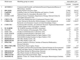
Table 1Description of the 23 CMIP5 coupled models analysed in this study. Names in bold indicate the model retained for the evaluation of ITV (Sect. 3.2).
Other studies have focused on the assessment of the ITV in the CMIP databases. Hung et al. (2013) evaluated the skill of 20 models from CMIP5 in simulating the MJO and convectively coupled equatorial waves (CCEWs) and compared their result with the one obtained from CMIP3 models (Lin et al., 2006). They showed that CMIP5 models exhibit an overall improvement in the simulation of ITV, especially the MJO and several CCEWs, as compared to CMIP3 models. The CMIP5 models produce larger total intraseasonal variance of precipitation than the CMIP3 models, including larger variances of MJO, Kelvin, ER and eastward inertio-gravity (EIG) waves. About one-third of the CMIP5 models generate the spectral peak of MJO precipitation between 30 and 70 days; however, the model MJO period tends to be longer than in the observations and only one of the 20 models is able to simulate a realistic eastward propagation of the precipitation patterns associated with MJO.
While the ITV and ENSO characteristics in CMIP5 have been documented separately, to the authors' knowledge, the evaluation of how the ITV relates to the El Niño cycle in CMIP5 models is lacking. This paper addresses this issue, incorporating recent progress in our understanding of ENSO, in particular its diversity (Capotondi et al., 2015). While a long-term motivation is to address the climate change issue, we are also guided by the will to identify the most skilful model in order to carry out process studies and document model biases within a physically based framework.
The paper is organised as follows.
The model database and the observed datasets used for the validation as well as the diagnostic methods used in this study are described in Sect. 2. The simulations of two types of El Niño, ITV components and the ITV ∕ ENSO relationship in CMIP5 models are analysed in Sect. 3. A summary and discussion are given in Sect. 4.
2.1 Data
The outputs of 23 models from the CMIP5 used for the Intergovernmental Panel on Climate Change (IPCC) Fifth Assessment Report (AR5) has been analysed (see model list in Table 1). The 250-year long simulations of the pre-industrial (hereafter PI) experiment (Taylor et al., 2012) are used for the evaluation of ENSO types, while a selected 20 years among these simulations are used to diagnose the ITV characteristics. The motivation for focusing on the PI experiment and not on the historical simulations as it is commonly done for model evaluation stands in the fact that it eases the interpretation of the results since there is no external forcing in the PI experiments, which provides a benchmark for further assessment of the sensitivity of the ENSO ∕ ITV relationship to climate change in the CMIP5 models. Monthly-mean sea surface temperature (SST) over a 250-year period and daily-mean zonal wind at 850 hPa over selected chunks of 20 years with daily data are used. Taking into account the decadal modulation of the ITV ∕ ENSO relationship, the data of the historical simulations were used for the statistical analysis of the ITV ∕ ENSO relationship, which presents data with daily resolution over a longer period than 20 years. A total of 66 years were used for the analysis (1950–2005). For comparison of the results with observations, the Hadley Centre Global Sea Ice and Sea Surface Temperature (HadISST, Rayner et al., 2003) archive and the National Centers for Environmental Prediction (NCEP)/National Center for Atmospheric Research (NCAR) Reanalysis (Kalnay et al., 1996) zonal wind at 850 hPa are used.
2.2 Methods
To document the ITV properties, we use the technique proposed by Wheeler and Kiladis (1999). This method is identical to those used in previous studies evaluating the realism of MJO and CCEW in CMIP3 (Lin et al., 2006) and CMIP5 (Hung et al., 2013) models. It is based on the decomposition of the symmetric and antisymmetric components relative to the Equator components of the field in the frequency–wavenumber space. Inversed Fourier transform is then used to recompose the signal in the desired frequency and wavenumber bands. The frequency and wavenumber intervals were derived from the normalised space–time spectrum for U850 and are centred on the spectral maximum of U850 (see Gushchina and Dewitte, 2011). In the models, the localisation of spectral maximum may differ from the reanalysis. However, sensitivity tests show that slight changes in the frequency–wavenumber interval do not significantly change the characteristics of the recomposed signal; therefore, fixed boundaries in the frequency and zonal wavenumber domain were used. These are, for MJO, zonal wavenumbers 1–3 and a period of 30–96 days; for equatorial Rossby waves, zonal wavenumbers and a period of 10–50 days, with negative (positive) zonal wavenumbers corresponding to the westward-propagating (eastward-propagating) waves. For Rossby waves, the frequency–wavenumber bands are also limited by the dispersion curves corresponding to values of the atmosphere equivalent depth ranging from 8 to 90 m, which follows Wheeler and Kiladis (1999).
Following Hayashi (1979), only the part of the eastward power that is incoherent with its equivalent westward power represents the true eastward-propagating signal. Moreover, the results of Jiang et al. (2015) emphasise the dominant stationary signals in many model simulations. To verify if the westward counterpart is present in the models, we recomposed the signal in the same frequency intervals as for MJO and Rossby waves but for the opposite sign of zonal wavenumbers: for MJO and for Rossby waves. Insignificant correlation between westward and eastward signals confirms that westward and eastward parts are incoherent, validating a posteriori our decomposition approach of the model outputs.
The amplitude of ER and MJO was calculated by taking the root mean square (rms) of the recomposed signal in a running window whose span depends on the wave's type (90 and 48 days for MJO and equatorial Rossby waves, respectively). Then, the running rms was considered as monthly averaged. To calculate the anomalies, the mean climatology over the investigated period was removed.
We use here U850 field for ITV filtering instead of outgoing longwave radiation (OLR) or brightness temperature signals from satellite data that are commonly used to derive the frequency–wavenumber of ITV, noting that the filter bands are similar for OLR and U850 as predicted by a simple dynamical model of ITV (Thual et al., 2014). Moreover, the use of zonal wind field eases the interpretation of the results since it is the westerly wind anomalies that serve as a physical conduit from the ITV to the ENSO dynamics. This approach follows previous relevant studies (McPhaden et al., 2006; Hendon et al., 2007).
In order to depict ENSO variability in terms of its two flavours (or regimes), we used the indices defined by Takahashi et al. (2011), the so-called E and C indices, that consist in the linear combination (through rotation) of the first two EOFs of the SST anomalies over the tropical Pacific (20∘ S–20∘ N; 120∘ E–80∘ W). Whereas the E index accounts for the extreme El Niño events that are of EP type, the C index grasps the variability associated with the CP El Niño and La Niña events. These indices, independent by construction (i.e. their correlation is zero), can be conveniently used for correlation or regression analyses. In particular, we infer the mode patterns associated with the two types of El Niño by bilinearly regressing the SST anomalies over the tropical Pacific onto the E and C indices. These mode patterns have a more consistent physical interpretation than the mode patterns associated with the first two EOF modes of SST anomalies over the tropical Pacific (see Takahashi et al., 2011 for details).
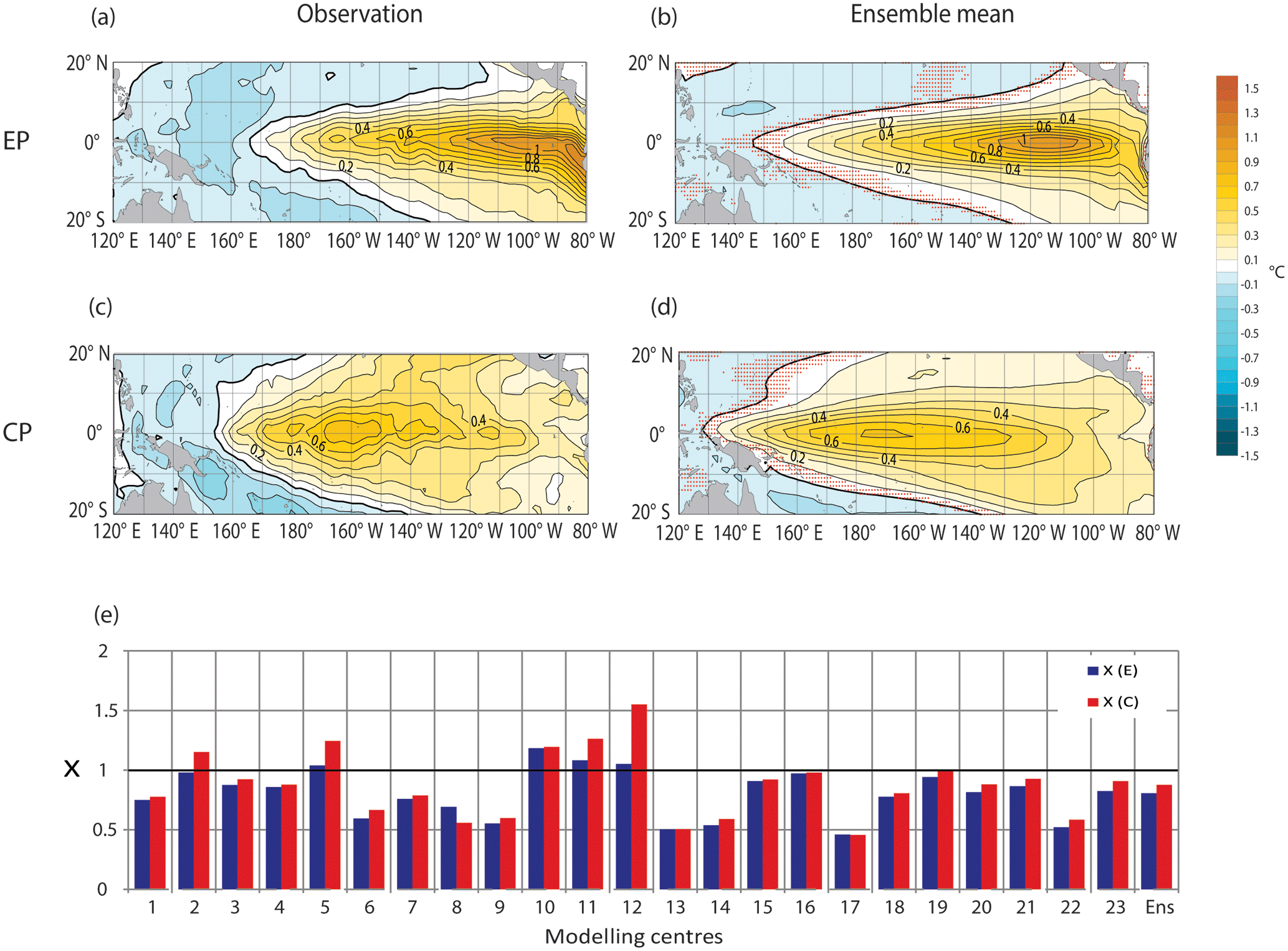
Figure 1E and C mode patterns (i.e. regression of SST anomalies onto the E and C indices) for (a, c) the observations and (b, d) the ensemble mean of the CMIP5 models (see Table 1 for the model names). The estimate from the models is based on 250 years of the PI control experiment. Stippling (red dots) indicates where the sign of the E and C patterns differs among the models by 70 %. (e) Histogram of the quantity X is defined as for the different models and the ensemble mean and where Y is either E or C. X is thus a metric of the model skill in accounting for the spatial pattern and amplitude of the E and C modes. Blue (red) refers to the E (C) mode.
The CP and EP events were selected using the time series of E and C indices. The E∕C index above 0.75 times their standard deviation during at least 3 consecutive months of the winter period (October–March) defines EP/CP El Niño events.
3.1 The two flavours of El Niño
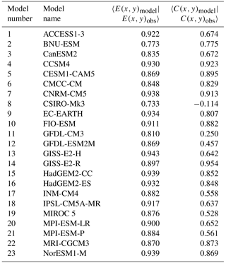
As a first step, the models' skill in simulating ENSO diversity is assessed based on the comparison of the E and C modes with those of observations. The E and C patterns for the ensemble mean of the 23 CMIP5 models (see Table 1 for the list of models) and for the observations (HadISST dataset) are presented in Fig. 1. As a metric of the skill of the model in accounting for the amplitude and pattern of the modes, we estimate the projection of model pattern onto the observed one within 10∘ S–10∘ N (bottom panel of Fig. 1). Figure 1 indicates that the model ensemble is quite realistic in accounting for the two types of El Niño in terms of their spatial pattern. The ensemble mean hides however some dispersion among models that is illustrated in Fig. 1e. The discrepancy between the models and observation in terms of the X value (see formula in the caption) is due to the model's tendency to have a SST anomaly pattern shifted to the west compared to the observations (Kim and You, 2012; Ham and Kug, 2012) but also due to the differences in the amplitude of the mode patterns, which is related to the deficiency of the models in accounting realistically for the ENSO asymmetry (Zhang and Sun, 2014) and non-linearity (Karamperidou et al., 2017). In general, though, the models simulate a reasonable ENSO period (not shown), in particular, with a shorter period of the E index (∼ 3–6 years) than the C index (∼ 5–8 years), in agreement with the observations. The objective classification of the models is difficult considering the number of other important ENSO properties to consider (e.g. seasonal phase locking, asymmetry, amplitude modulation, relative contribution of feedbacks) than just its diversity. We have also to consider a compromise between the model skill in realistically simulating ENSO properties and ITV (see next section). For simplicity, and considering the dispersion in ENSO amplitude among models, we thus decide to quantify the model skill in simulating ENSO diversity based on a simple metric consisting in the spatial correlation of the E and C patterns between the observations and models within 5∘ S–5∘ N (Table 2) and consider that the model is “realistic” enough if the value of this metric is above 50 %. This excludes three models from the subsequent analyses: GFDL-CM3, GFDL-ESM2M and CSIRO-Mk3. We will see hereafter that the evaluation of ITV in the models yields a more stringent test of the model realism, which will reduce drastically the number of models for the assessment of the ENSO ∕ ITV relationship (Sect. 3.3).
Table 2Spatial correlation between observed (HadISST) and simulated (CMIP5 models) E and C patterns within the equatorial Pacific (120∘ E–80∘ W; 5∘ S–5∘ N).
3.2 Intraseasonal tropical variability
The characteristics of ITV are documented here with the focus on its intensity, seasonality and propagating features. Earlier studies have evidenced biases in the simulation of MJO and CCEW in CMIP models (Guo et al., 2015; Jiang et al., 2015; Klingaman et al., 2015; Xavier et al., 2015), however, with the CMIP5 models being more realistic (Hung et al., 2013) than the CMIP3 models (Lin et al., 2006). Our analysis here is based on the most realistic models in terms of their skill in simulating the two types of El Niño. Some modes are not considered in the analyses because the daily data of U850 were not available in open access. We thus retain 16 models: ACCESS1-3, BNU-ESM, CanESM2, CCSM4, CMCC-CM, CNRM-CM5, EC-EARTH, HadGEM2-CC, HadGEM2-ES, INMCM4, IPSL-CM5A-MR, MIROC5, MPI-ESM-LR, MPI-ESM-P, MRI-CGCM3 and NorESM1-M. The 20 years of the PI experiment for each model are analysed, the results of which are compared to the NCEP/NCAR Reanalysis data over the period 1980–1999.
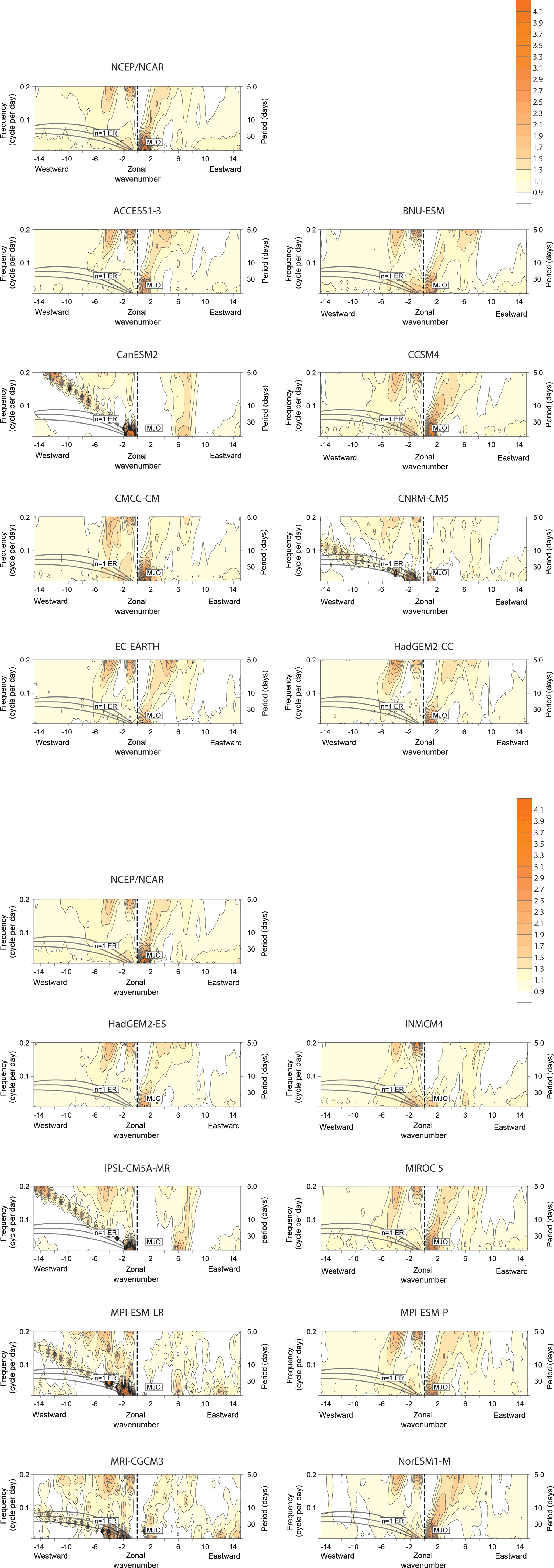
Figure 2Space–time spectrum averaged between 15∘ N and 15∘ S of the symmetric component of U850 divided by the background spectrum for the NCEP/NCAR Reanalysis and the CMIP5 models.
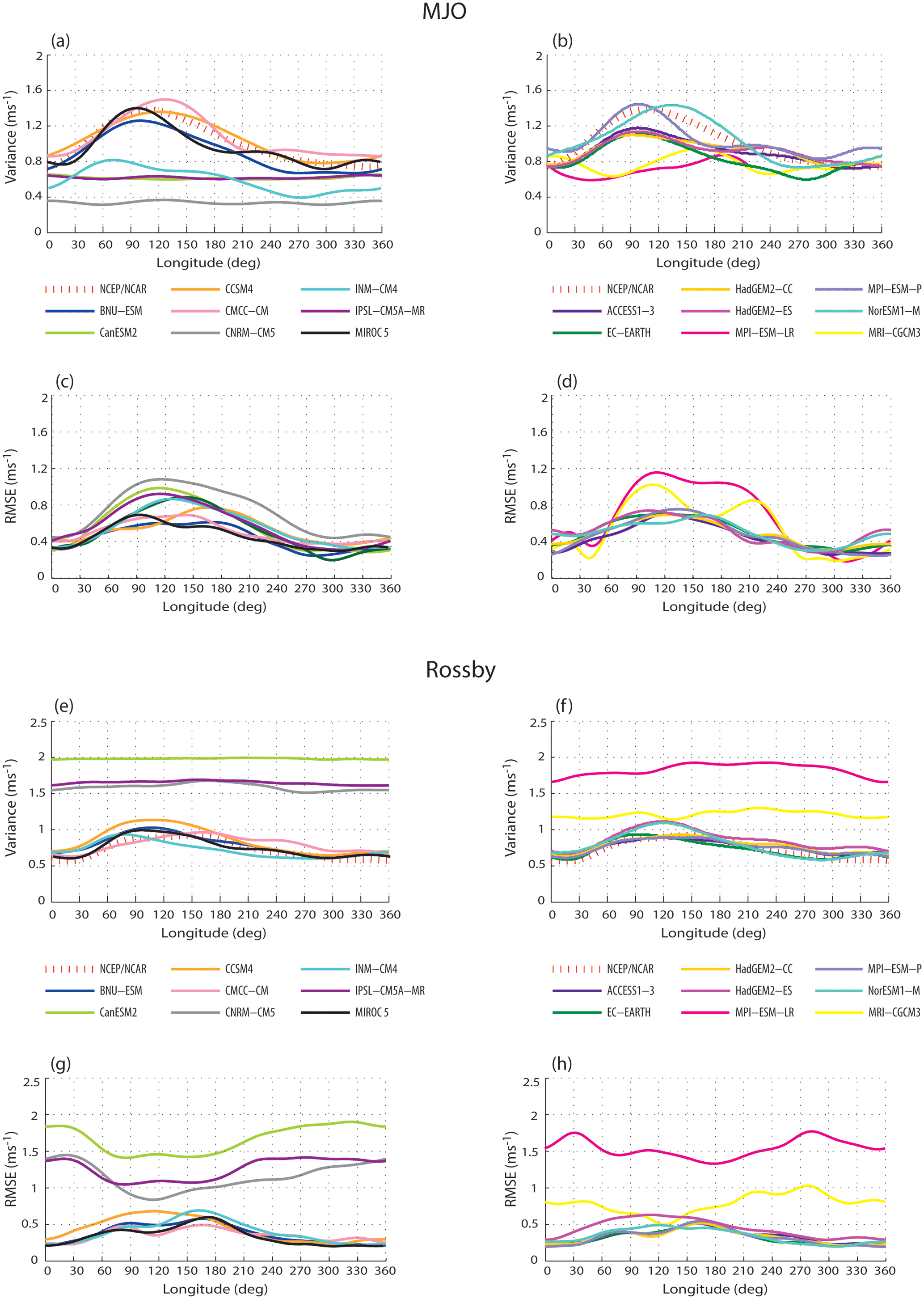
Figure 3Variance (rms) of MJO (a, b) and Rossby waves (e, f) filtered U850 averaged between 15∘ N and 15∘ S for CMIP5 models and the NCEP/NCAR Reanalysis. Root mean square error (RMSE) between modelled and observed variance of MJO (c, d) and Rossby waves (g, h) averaged between 15∘ N and 15∘ S.
Table 3Summary of the model skill according to the diagnostics performed in our study. The + and − signs refer to “semi-objective” criteria which are defined in Table 4. The model names in bold are those analysed in Sect. 3.3 (i.e. seasonal ENSO ∕ ITV relationship).
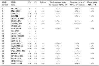
Table 4Definition of the scale for classifying the models' skill for Table 3.
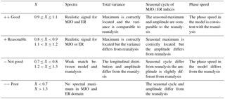
Figure 2 presents the space–time spectra normalised above the background spectra for the symmetric component of U850 wind for the observations (Fig. 2, upper panel) and for the CMIP5 models. Superimposed upon these plots are the dispersion curves for the odd meridional mode number of equatorial waves for various equivalent depths (h=12, 25 and 50 m). A total of 11 models out of 16 are capable of simulating the eastward-propagating MJO signal with maximum at zonal wavenumber 1 in relatively good agreement with the observations. However, the intensity of the MJO-associated spectral maximum differs among the models. A total of five models out of 16 simulate unrealistic westward-propagating disturbances with zonal wavenumbers 1–3. Seven models (BNU-ESM, CCSM4,3 CMCC-CM, INM-CM4, MIROC5, MPI-ESM_P and Nor ESM1-M) simulate a realistic ER spectral maximum (Fig. 2).
Figure 4Seasonal variances (rms) of MJO averaged zonally over the tropical Pacific (120∘ E–90∘ W) and meridionally over (a, b) 10–15∘ N, (c, d) 5∘ N–5∘ S and (e, f) 10–15∘ S for the NCEP/NCAR Reanalysis and the models.
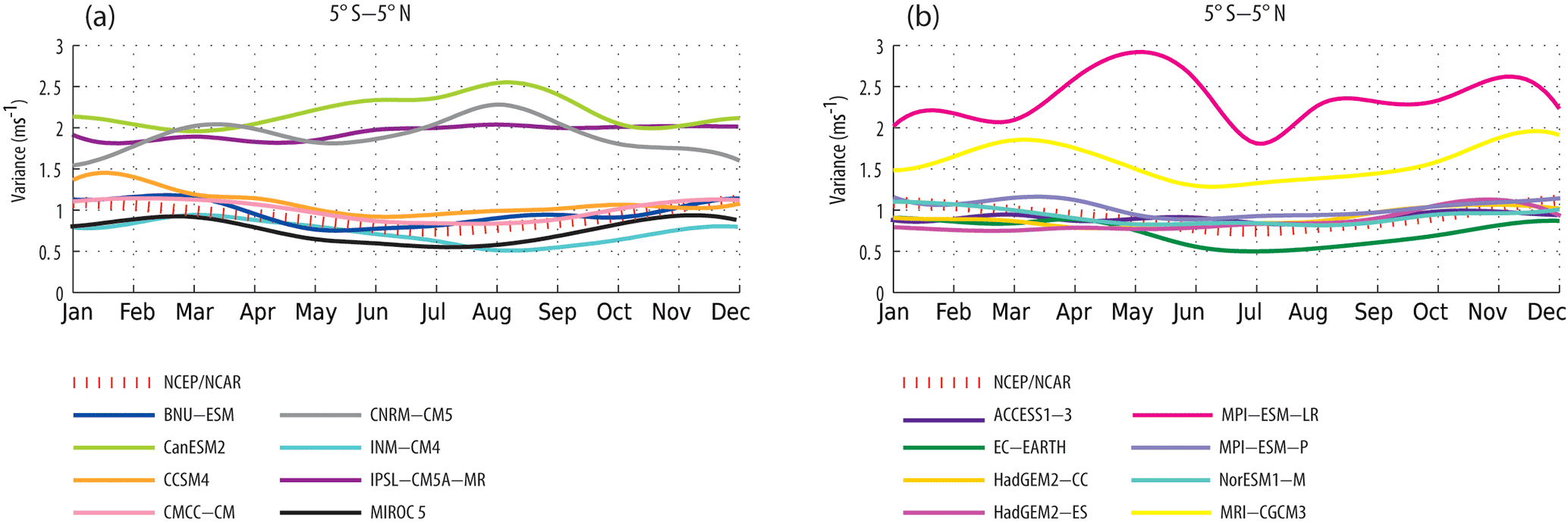
Figure 5Seasonal variances (rms) of Rossby waves averaged zonally over the tropical Pacific (120∘ E–90∘ W) and meridionally over 5∘ S–5∘ N for NCEP/NCAR Reanalysis and the CMIP5 models.
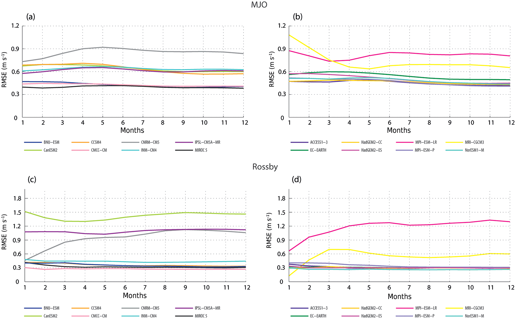
Figure 6Root mean square error (RMSE) between modelled and observed seasonal variance of MJO (a, b) and Rossby waves (c, d) averaged zonally over the tropical Pacific (120∘ E–90∘ W) and meridionally over 5∘ S–5∘ N.
The distribution of the variance of the MJO and ER along the equatorial band is also key to accounting for the relationship between ENSO and ITV considering that the balance between oceanic feedbacks which depends on the sloping mean thermocline determines the nature of the coupled instability during ENSO (An and Jin, 2001). The rms values of the ITV components over 20 years averaged between 15∘ N and 15∘ S were plotted as a function of longitude for the models and the NCEP/NCAR Reanalysis (Fig. 3a, b, e, f). The location of the MJO maximum in the eastern Indian Ocean and western Pacific is relatively realistically simulated by ACCESS1-3, BNU-ESM, CCSM4, CMCC-CM, EC-EARTH, HadGEM2-CC, HadGEM2-ES, MIROC5, MPI-ESM-P and NorESM1-M models. In particular, these models have a root mean square error (RMSE) that is ∼ 50 % of the variance of the NCEP/NCAR data in the tropical Pacific region (Fig. 3c, d). However, in CMCC-CM and NorESM1-M, the maximum is shifted toward the central Pacific, while ACCESS1-3, HadGEM2-CC, HadGEM2-ES and EC-EARTH underestimate the total MJO variance in the eastern Indian and western Pacific oceans. CanESM2, CNRM-CM5, IPSL–CM5A–MR, MPI-ESM-LR and MRI–CGCM3 do not exhibit a significant peak in the eastern Indian and western Pacific oceans which may be critical for the proper simulation of the relationship between ITV and oceanic Kelvin wave activity. Nine models out of 16 models simulate a relatively realistic magnitude and longitudinal distribution of ER variance (Fig. 3e, f) associated with a relatively weak RMSE (Fig. 3g, h). It is noteworthy that the ER variance maximum in the central Pacific is correctly simulated by ACCESS1-3, CMCC-CM, HadGEM2-CC and HadGEM2-ES. As a summary of the results, Table 3 synthesises the models' skill in the various diagnostics carried out in this study. Since it is mainly based on the visual appreciation of the figures and thus somehow subjective, Table 3 is mostly provided for clarity and readability.
In the following, the seasonality of the ITV is assessed considering the focus of this study on the seasonal dependence of the ENSO ∕ ITV relationship.
The MJO has a maximum intensity in the summer hemisphere (i.e. in the Northern Hemisphere in July and in the Southern Hemisphere in January), which implies that the MJO variance peaks along the Equator in boreal spring (Zhang and Dong, 2004) when it may act efficiently as an ENSO trigger. Therefore, the MJO cross-equatorial seasonal migration is a key feature that needs to be realistically simulated in the models. The MJO seasonal variability is thus estimated over the three latitudinal belts: 10–15∘ N, 5∘ N–5∘ S and 10–15∘ S (Fig. 4). For ER, since its variance remains confined to the equatorial band all year long, its seasonal cycle is estimated in the 5∘ N–5∘ S belt only (Fig. 5). In the NCEP/NCAR Reanalysis, the MJO exhibits a larger variability in the summer hemisphere with a higher amplitude in the Southern Hemisphere than in the Northern Hemisphere. In the northern tropical Pacific (10–15∘ N), the MJO activity peaks from June to September (Fig. 4a, b), while in the southern tropical Pacific (15–10∘ S), it peaks from November to March (Fig. 4e, f). In the near-equatorial area, there is no marked seasonal peak, but a slight intensification from November to April and a relaxation from May to October are observed (Fig. 4c, d). The seasonal shift of the MJO maximum drastically differs among the models. The comparison of the models to the observations indicates that HadGEM2-CC, ACCESS1-3, MPI-ESM-P, CMCC-CM, BNU-ESM and MIROC5 are the models that simulate the MJO seasonal cycle the most realistically since they have the smallest values of RMSE along the Equator (Fig. 6a). The CCSM4, NorESM1-M and INM-CM4 models simulate the correct timing of the seasonal maximum but with lower MJO amplitude for INM-CM4 and larger amplitude for CCSM4 and NorESM1-M as compared to the observations. The seasonal cycle of ER is reasonably simulated by BNU-ESM, CCSM4, CMCC-CM, HadGEM2-CC, HadGEM2-ES, INMCM4, MIROC5 and NorESM1-M (Figs. 5a, b and 6). The reader is invited to refer to Table 3 for a summary of the models' skill in simulating ITV seasonality.
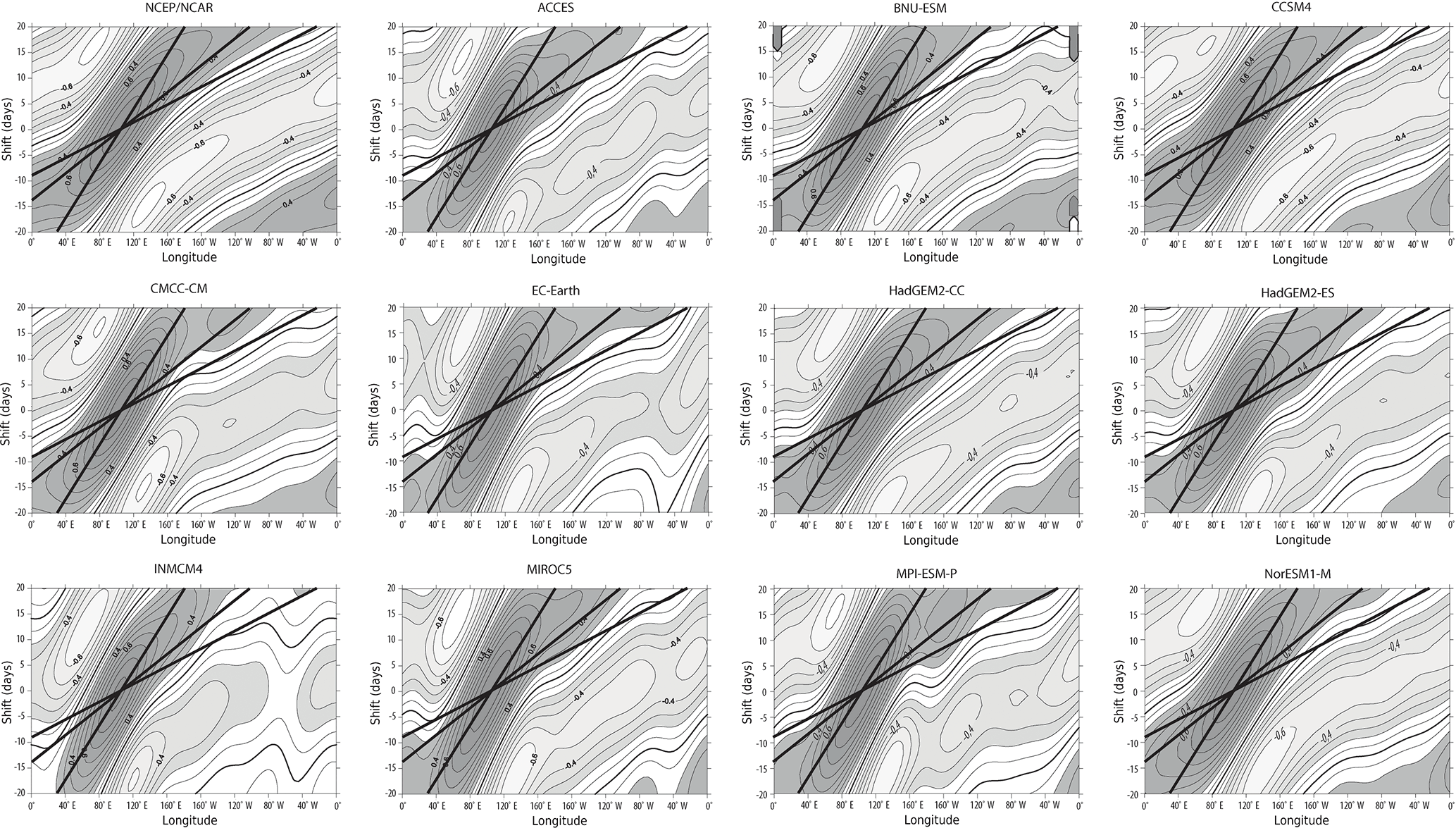
Figure 7Lag correlation of the MJO filtered U850 averaged along the Equator between 5∘ N and 5∘ S with respect to itself at the Equator and 105∘ E for the NCEP/NCAR Reanalysis and the CMIP5 models. The three diagonal lines correspond to phase speeds of 5, 10 and 15 m s−1.
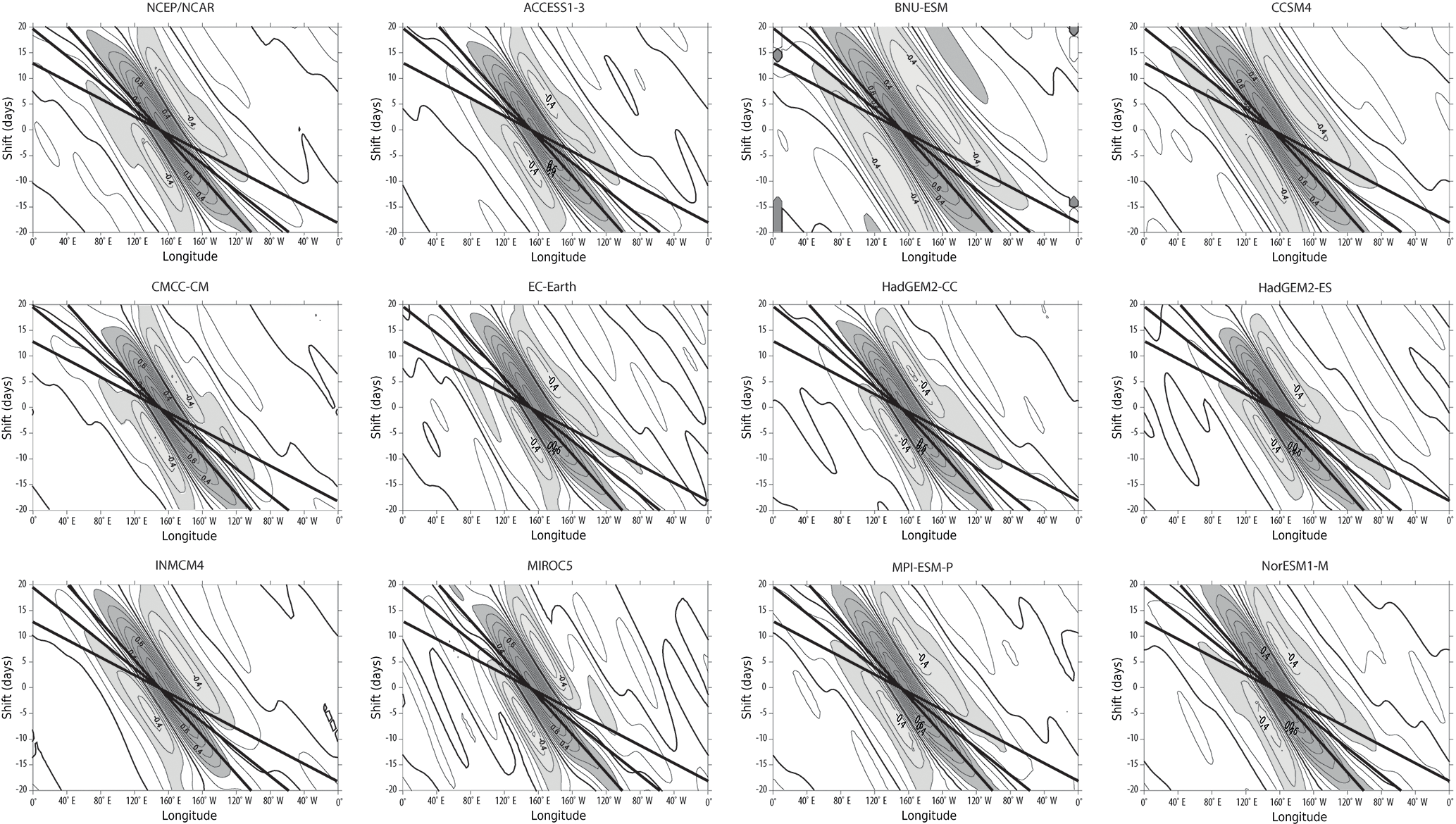
Figure 8Lag correlation of the ER filtered U850 averaged along the Equator between 5∘ N and 5∘ S with respect to itself at the Equator and 150∘ E for the NCEP/NCAR Reanalysis and the CMIP5 models. The three diagonal lines correspond to phase speeds of 7, 10 and 15 m s−1.
Further, the propagating characteristics of the MJO and ER along the Equator are documented for the most skilful models in terms of the amplitude and seasonal cycle of the ITV. Figures 7 and 8 show the lag correlation of the MJO and ER filtered U850 time series averaged between 5∘ N and 5∘ S with respect to itself at the Equator and 105∘ E for MJO and 150∘ E for ER, respectively. Superimposed upon these plots are the lines corresponding to phase speeds of 5, 7, 10 and 15 m s−1. The observation evidences an eastward-propagating MJO pattern with a phase speed of about 5 m s−1 (Fig. 7). A total of six models out of 11 display propagation characteristics that are consistent with the observations. The MJO phase speed is slightly slower than in observations in CMCC-CM, EC-EARTH, INM-CM4, MIROC5 and MPI-ESM-P. Note that Hung et al. (2013), who documented the MJO signal from precipitation data, found a very slow propagation in most CMIP5 models, which is not the case here for the MJO-associated patterns of the low troposphere winds. The Rossby wave propagates westward with phase speed around 7 m s−1 to the west of the dateline and 5 m s−1 to the east of the dateline in the observations. Eight models simulate a realistic Rossby wave phase speed value, while three models (CMCC-CM, INM-CM4 and NOR-ESM1-M) simulate a too slow phase speed (Fig. 8).
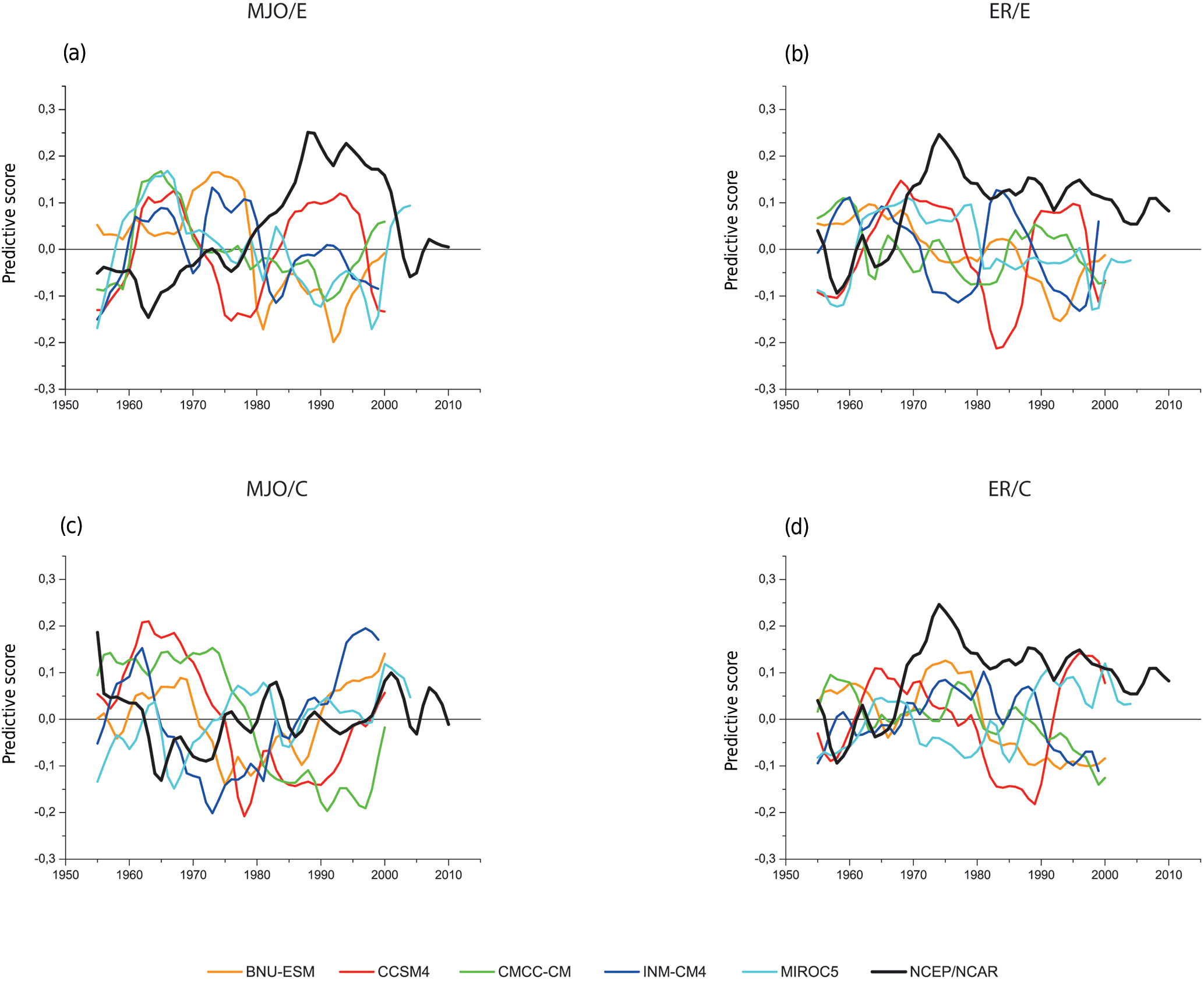
Figure 9Evolution of the predictive score (see Eq. 1 in the text) for MJO (a, c) and ER (b, d) and for EP (a, b) and CP (c, d) El Niño events for five CMIP5 models and the NCEP/NCAR Reanalysis. Note that the mean was removed for the models but not for the observations.
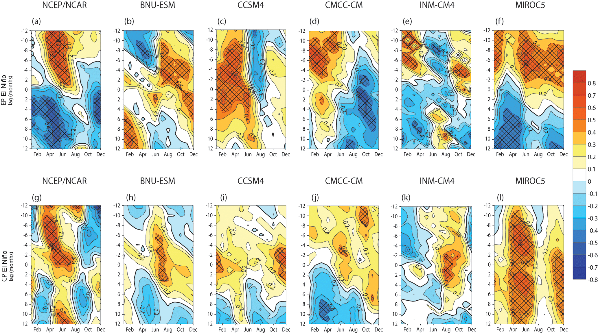
Figure 10Monthly lagged correlation of E (a–f) and C (g–l) indices as a function of start month with respect to MJO activity index for NCEP/NCAR Reanalysis and five CMIP5 models. Contour interval is 0.1. Negative correlation is blue shaded, positive correlation is orange shaded. Hatching lines denote correlation at the 90 % statistical confidence level based on Gaussian statistics. The thick black line indicates the zero correlation line.
3.3 ITV ∕ ENSO seasonal relationship
In this section, our objective is to illustrate the large dispersion among models' skill in simulating the ITV ∕ ENSO relationship, despite an overall good skill in simulating ITV and ENSO diversity separately for some of them. We thus arbitrarily select five models among the “good” models (see Table 3). One difficulty for assessing the ITV ∕ ENSO relationship is associated with the fact that it can experience a low-frequency modulation. Gushchina and Dewitte (2018) showed in particular that there is a significant decadal variability of the ITV ∕ ENSO relationship over the observational record (see Fig. S1), which arises either from change in mean state impacting the ENSO dynamics or changes in the properties of ITV itself. Thus, in order to take into account such a decadal modulation, the 11-year running mean of the lagged correlation between the MJO and ER activity indices in the equatorial Pacific and the E and C indices in January is first assessed in order to determine the periods (in the historical runs) when the statistics are robust (see Fig. S2 for an example for the CMCC-CM model). The MJO and ER indices are calculated as the running variance of U850, filtered in the domain of MJO and ER, averaged over the regions where the maximum of the ITV ∕ ENSO relationship is observed in reanalysis (Gushchina and Dewitte 2011): western Pacific (120–180∘ E; 5∘ S–5∘ N) for MJO and central Pacific (140∘ E–160∘ W; 5∘ S–5∘ N) for Rossby waves. In order to select the periods, following Gushchina and Dewitte (2018), we define a measure of the “predictive skill” of either the MJO or ER with respect to ENSO. It is defined as follows:
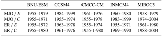
where represents the correlation as a function of time (t) and time lag (τ) between the ENSO index (either E or C indices) in Jan(0) (i.e. at the ENSO peak) and the considered month of ITV (either MJO or ER) activity. within the integral is set to zero when it is not statistically significant at the 95 % confidence level. is thus the weighted ITV ∕ ENSO correlation between Mar(−1) and Jan(0) which gives larger weight to correlation at large time lags (1 in Mar(−1)) and little at short lags (0 in Jan(0)), and can therefore be interpreted as a measure of the predictive value of either MJO and ER with regards to the E and C indices. The time series of , , and for the model and the observations are provided in Fig. 9. For the following diagnostic, we identify the period of a strong MJO ∕ E(C) and ER ∕ E(C) relationship as a period with positive predictive score during at least 16 years (in accordance with the observations where the period of a strong ITV ∕ C relationship is 2000–2015). Note that the mean over the full period was removed in the models for comparison between them but not in the observations (for comparison with Gushchina and Dewitte, 2018). The observations exhibit higher values of the predictive score than the model anyway (see also the Supplement). In some models, there is no extended period of time (i.e. period longer than 16 years) when the value of the predictive score is positive over the whole record. In this case, we choose to consider a 16-year period centred on the peak value of the predictive score. The periods used for the subsequent lag correlation analysis are provided in Table 5. The reference period for the NCEP/NCAR Reanalysis is 1979–1998 for EP El Niño and 2000–2015 for CP El Niño, selected as a period of occurrence of mostly EP or CP El Niño events, respectively. The lagged correlation between the C and E indices with respect to the MJO and ER activity indices is then calculated as a function of calendar month (Figs. 10 and 11).
Consistently with the results conveyed in Fig. 9, the ITV ∕ ENSO relationships associated with the two types of El Niño events are very diverse among models, and do not compare in a straightforward manner with the observations. In the observations, the MJO activity in March–July is ahead of the peak SST anomalies (correlation greater than 0.6) by 4 to 12 months (3 to 9 months) during the EP (CP) El Niño events (Fig. 10a, g). The significant positive correlation persists up to positive time lags (MJO lags SST) during the CP El Niño event, mirroring the strong MJO after the SST peak. During the EP El Niño event, the MJO precursor signal is present in all models but the correlation is lower in BNU-ESM and INMCM4 as compared to the observations (Fig. 10b, e), while MIROC5 and BNU-ESM simulate shorter time lag between MJO intensification and SST rise (Fig. 10b, f). Note that all models except for MIROC5 exhibit a too strong MJO intensity after the El Niño peak (positive correlation at positive time lags). The MJO intensification prior to the CP El Niño event is also simulated by all models (Fig. 10h–l), however, with a different timing than the observations. In MIROC5, the pattern of the lag correlation is the most realistic amongst the models (correlation in the lag–month space between observations and models reaches 0.45, 0.38, −0.01, −0.06 and −0.06 for MIROC5, BNU-ESM, CCSM4, CMCC-CM and INM-CM4, respectively). Although the precursor signal is simulated by BNU-ESM, the correlation values prior to the ENSO peak are lower than in the observations. In CCSM4 and CMCC-CM, the MJO ∕ C correlation is weak prior to the ENSO peak (Fig. 10i, j). INM-CM4 simulates the strongest simultaneous correlation between the MJO and C indices, while the precursor signal is rather weak (Fig. 10k).
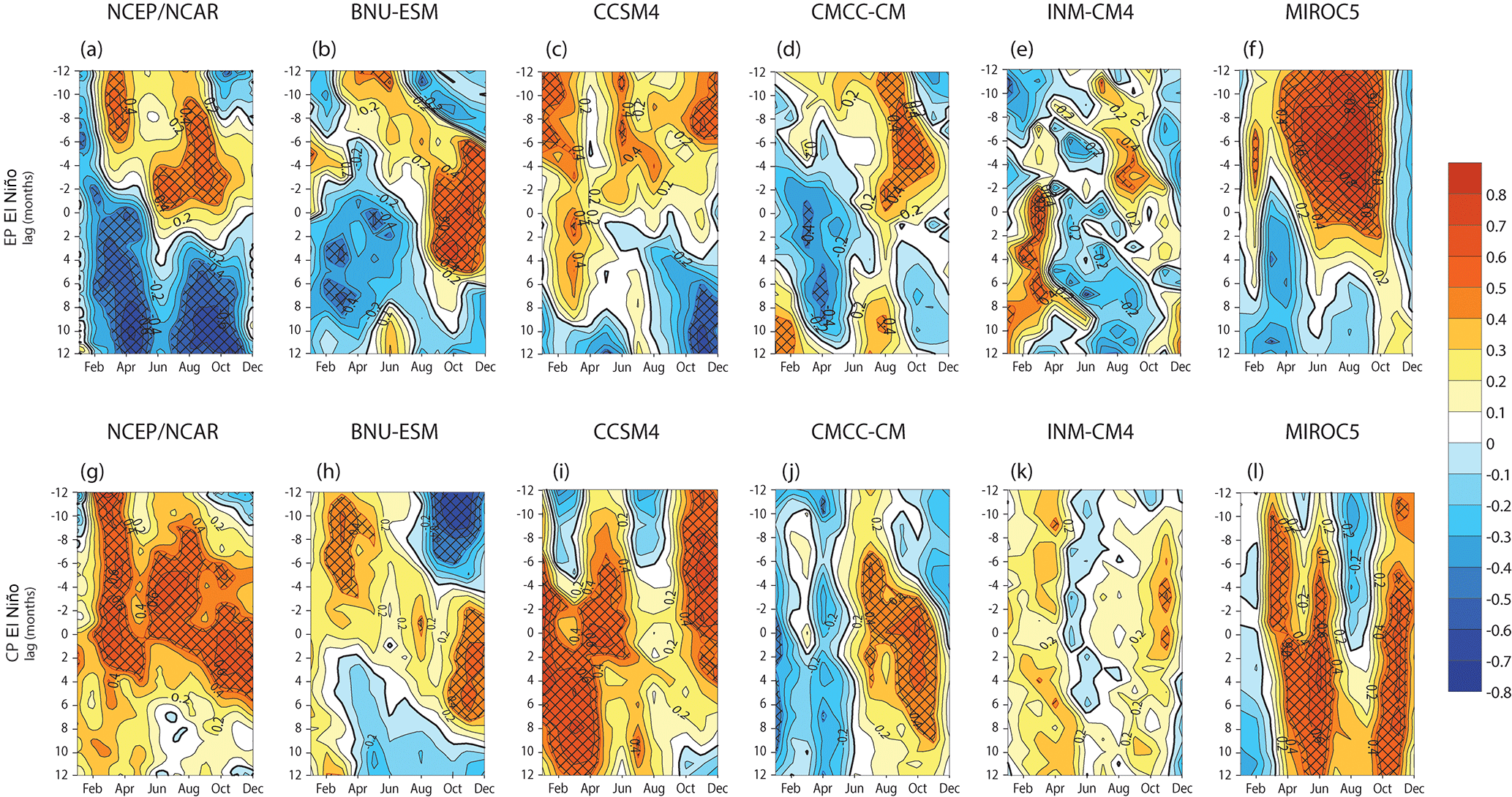
Regarding the Rossby wave, the observations indicate that the ER activity intensifies in February–April and July–September of the year prior to the EP El Niño peak (Fig. 11a). During CP El Niño, the Rossby wave activity also appears to be a good precursor, and the relationship with SST anomalies persists after the peak phase (Fig. 11g). All five models have some skill in simulating the ER ∕ ENSO relationship. However, INM-CM4 does not simulate the peak of ER in February–April (Fig. 11e), MIROC5 has a too strong and persistent correlation between the ER and E indices (Fig. 11f), while BNU-ESM and CCSM4 have differences with the observations in terms of the period of the calendar year when the ITV ∕ ENSO relationship is the strongest (Fig. 11b, c). CMCC-CM exhibits the most realistic features (Fig. 11d). All models simulate the increased ER activity prior to and after the CP El Niño peak but the values of correlation are smaller and the timing of the peak correlation is different from the observations (Fig. 11g–l).
In this paper, we question the extent to which the models that are used for assessing the change in ENSO properties under global warming (i.e. CMIP5) are able to account for a fundamental ENSO property found in the observations, that is, the tendency of ITV activity to increase one to two seasons prior to the ENSO peak (McPhaden et al., 2006; Hendon et al., 2007; Gushchina and Dewitte, 2012). Five CMIP5 models (BNU-ESM, CCSM4, CMCC-CM, INM-CM4 and MIROC5) are retained that have been evaluated among a total of 16 that exhibit relatively good skills in simulating many aspects of the ITV, that is, its variance along the Equator, its seasonality and the propagation characteristics of the MJO and ER. These five models have also some skills in accounting for the so-called ENSO diversity, that is, the existence of two types of El Niño events, the EP and CP events. Despite the ability of these models to simulate relatively realistically both the ITV characteristics and the ENSO diversity, they exhibit limited skill in simulating the seasonal ENSO ∕ ITV relationship. In particular, a large dispersion among these five models is found in terms of the lag correlation between ITV and the two ENSO indices accounting for both types of events (Figs. 10 and 11). Noteworthy, still, is that the models capture distinct patterns of the MJO and ER activity in relation to the two types of events. The limited skill in terms of the ENSO ∕ ITV relationship of the models raises concerns on many aspects. First, it questions the extent to which ENSO in the models is influenced by other forms of external forcings not necessarily related to the ITV. This would be consistent with recent studies (Dommenget and Yu, 2018; Takahashi et al., 2018) that suggest that ENSO is likely to be more influenced by external forcing than previously thought. In particular, Takahashi et al. (2018) shows, based on the experimentation with a conceptual non-linear recharge–discharge model, that the role of the low-frequency component of the external forcing (interannual timescales) is actually key to triggering El Niño events and that there can be extreme El Niño events without a significant recharge of the heat content. What happened in 2014, when a strong El Niño event was expected after strong WWEs in February–March similar to 1997 (Menkes et al., 2014), was also the indication that external forcing is key for the development of El Niño independently of whether or not the deterministic recharge–discharge process is at work (Hu and Fedorov, 2016; Levine and McPhaden, 2016). There is also a large body of literature showing the influence of remote regions from the tropical Pacific on ENSO (e.g. You and Furtado, 2017, among many others). Within the tropical Pacific, ENSO can be influenced by the so-called meridional mode that operates through wind–evaporation–SST feedback either in the Northern Hemisphere (Vimont et al., 2001; Chiang and Vimont, 2004; Yu and Kim, 2011; Larson and Kirtman 2013) or the Southern Hemisphere (Zhang et al., 2014). Therefore, ENSO precursors/triggers are not limited to the ITV and its projection on the ocean wave dynamics. Our results thus suggest that external forcing of ENSO in the CMIP5 models may be not predominantly through ITV. Another related aspect is that ITV may not be just an additive forcing for ENSO but can be considered a state-dependent noise forcing (Jin et al., 2007). In reanalysis data, its amplitude was also shown to be critical for the ENSO amplitude modulation (Kug et al., 2008; Levine and Jin, 2015). Interestingly, Levine et al. (2016) demonstrated that CMIP5 models are unable to correctly simulate the state-dependent noise forcing of ENSO, which may involve the model inability to reproduce the ITV ∕ ENSO seasonal dependence. Further investigation is required to relate the statistical analysis of the nature (i.e. additive versus multiplicative) of the atmospheric forcing to the mechanistic understanding of how the atmospheric forcing is modulated by mean state conditions. This would be critical for advancing on the physical interpretations of the statistical results based on the sensitivity of the CMIP models to global warming, such as the doubling in the occurrence of extreme El Niño events in the future in response to greenhouse warming (Cai et al., 2015).
The codes in Fortran and MATLAB are available from the corresponding author upon request (Daria Gushchina, dasha155@mail.ru).
Model data can be downloaded from the CMIP (Coupled Model Intercomparison Project) data portal (https://cmip.llnl.gov/cmip5/data_portal.html).
The supplement related to this article is available online at: https://doi.org/10.5194/gmd-11-2373-2018-supplement.
This study is supported by the Russian Foundation of Basic Research grant
nos. 18-05-00767 and 16-35-00394/16. The study is carried out in the
framework of the scientific program of Faculty of Geography of Moscow State University
(no. AAAA-A16-116032810086-4). Boris Dewitte acknowledges supports from
FONDECYT (grant nos. 1151185 and 1171861) and from LEFE-GMMC.
Edited by: Richard Neale
Reviewed by: three
anonymous referees
An, S.-I. and Jin, F.-F.: Collective role of zonal advective and thermocline feedbacks in ENSO mode, J. Climate, 14, 3421–3432, https://doi.org/10.1175/1520-0442(2001)014<3421:CROTAZ>2.0.CO;2, 2001.
Barnston, A., Tippett, M. K., L'Heureux, M. L., Li, S., and DeWitt, D. G.: Skill of real-time seasonal ENSO model predictions during 2002–2011: is our capability increasing?, B. Am. Meteorol. Soc., 93, 631–651, https://doi.org/10.1175/BAMS-D-11-00111.1, 2012.
Bjerknes, J.: A possible response of the atmospheric Hadley circulation to equatorial anomalies of Ocean temperature, Tellus, 18, 820–829, 1966.
Boulanger, J.-P., Menkes, C., and Lengaigne, M.: Role of high- and low-frequency winds and wave reflection in the onset, growth and termination of the 1997/1998 El Niño, Clim. Dynam., 22, 267–280, https://doi.org/10.1007/s00382-003-0383-8, 2004.
Cai, W., Santoso, A., Wang, G., Yeh, S.-W., An, S.-Il, Cobb, K. M., Collins, M., Guilyardi, E., Jin, F.-F., Kug, J.-S., Lengaigne, M., McPhaden, M. J., Takahashi, K., Timmermann, A., Vecchi, G., Watanabe, M., and Wu, L.: ENSO and greenhouse warming, Nat. Clim. Change, 5, 849–859, https://doi.org/10.1038/nclimate2743, 2015.
Capotondi, A., Ham, Y. G., Wittenberg, A. T., and Kug, J.-S.: Climate model biases and El Niño Southern Oscillation (ENSO) simulation, US CLIVAR Variations, 13, 21–25, 2015.
Chiang, J. C. H. and Vimont, D. J.: Analogous Pacific and Atlantic meridional modes of tropical atmosphere–ocean variability, J. Climate, 17, 4143–4158, 2004.
Choi, J., An, S. I., and Yeh, S. W.: Decadal amplitude modulation of two types of ENSO and its relationship with the mean state, Clim. Dynam., 38, 2631–2644, https://doi.org/10.1007/s00382-011-1186-y, 2012.
Diaz, H. F., Hoerling, M. P., and Eischeid, J. K.: ENSO variability, teleconnections and climate change, Int. J. Climatol., 21, 1845–1862, https://doi.org/10.1002/joc.631, 2001.
Dommenget, D. and Yu, Y.: The effects of remote SST forcings on ENSO dynamics, variability and diversity, Clim. Dynam., 49, 2605–2624, https://doi.org/10.1007/s00382-016-3472-1, 2018.
Fedorov, A.: The response of the coupled tropical ocean–atmosphere to westerly wind bursts, Q. J. Roy. Meteor. Soc., 128, 1–23, https://doi.org/10.1002/qj.200212857901, 2002.
Guo, Y., Duane, E., Waliser, and Xianan, J.: A systematic relationship between the representations of convectively coupled equatorial wave activity and the Madden–Julian oscillation in climate model simulations, J. Climate, 28, 1881–1904, https://doi.org/10.1175/JCLI-D-14-00485.1, 2015.
Gushchina, D. and Dewitte, B.: The relationship between intraseasonal tropical variability and ENSO and its modulation at seasonal to decadal timescales, Cent. Eur. J. Geosci., 1, 175–196, https://doi.org/10.2478/s13533-011-0017-3, 2011.
Gushchina, D. and Dewitte, B.: Intraseasonal tropical atmospheric variability associated with the two flavors of El Niño, Mon. Weather Rev., 140, 3669–3681, https://doi.org/10.1175/MWR-D-11-00267.1, 2012.
Gushchina, D. and Dewitte, B.: Decadal modulation of the ITV ∕ ENSO relationship and the two types of El Niño, Clim. Dynam., https://doi.org/10.1007/s00382-018-4235-y, online first, 2018.
Ham, Y.-G. and Kug, J.-S.: How well do current climate models simulate two types of El Niño?, Clim Dynam., 39, 383–398, https://doi.org/10.1007/s00382-011-1157-3, 2012.
Hayashi, Y.: A generalized method for resolving transient disturbances into standing and travelling waves by space–time spectral analysis, J. Atmos. Sci., 36, 1017–1029, https://doi.org/10.1175/1520-0469(1979)036<1017:AGMORT>2.0.CO;2, 1979.
Hendon, H. H., Wheeler, M. C., and Zhang, C.: Seasonal dependence of the MJO–ENSO relationship, J. Climate, 20, 531–543, https://doi.org/10.1175/JCLI4003.1, 2007.
Horel, J. D. and Wallace, J. M.: Planetary-Scale Atmospheric Phenomena Associated with the Southern Oscillation, Mon. Weather Rev., 109, 813–829, https://doi.org/10.1175/1520-0493(1981)109<0813:PSAPAW>2.0.CO;2, 1981.
Hung, M. P., Lin, J. L., Wang, W., Kim, D., Shinoda, T., and Weaver, S. J.: MJO and convectively coupled equatorial waves simulated by CMIP5 climate models, J. Climate, 26, 6185–6214, https://doi.org/10.1175/JCLI-D-12-00541.1, 2013.
Hu, S. and Fedorov, A. V.: An exceptional easterly wind burst stalling El Niño of 2014, P. Natl. Acad. Sci. USA, 113, 2005–2010, https://doi.org/10.1073/pnas.1514182113, 2016.
Jiang, X., Waliser, D. E., Xavier, P. K., Petch, J., Klingaman, N. P., Woolnough, S. J., Guan, B., Bellon, G., Crueger, T., DeMott, C., Hannay, C., Lin, H., Hu, W., Kim, D., Lappen, C. L., Lu, M. M., Ma, H. Y., Miyakawa, T., Ridout, J. A., Schubert, S. D., Scinocca, J., Seo, K. H., Shindo, E., Song, X., Stan, C., Tseng, W. L., Wang, W., Wu, T., Wu, X., Wyser, K., Zhang, G. J., ans Zhu, H.: Vertical structure and physical processes of the Madden-Julian oscillation: Exploring key model physics in climate simulations, J. Geophys. Res.-Atmos, 120, 4718–4748, https://doi.org/10.1002/2014JD022375, 2015.
Jin, F.-F.: An equatorial ocean recharge paradigm for ENSO, Part I: Conceptual model, J. Atmos. Sci., 54, 811–829, https://doi.org/10.1175/1520-0469(1997)054<0811:AEORPF>2.0.CO;2, 1997.
Jin, F.-F., Lin. L., Timmermann, A., and Zhao, J.: Ensemble-mean dynamics of the ENSO recharge oscillator under state-dependent stochastic forcing, Geophys. Res. Lett., 34, L03807, https://doi.org/10.1029/2006GL027372, 2007.
Kalnay, E., Kanamitsu, M., Kistler, R., Collins, W., Deaven, D., Gandin, L., Iredell, M., Saha, S., White, G., Woollen, J., Zhu, Y., Chelliah, M., Ebisuzaki, W., Higgins, W., Janowiak, J., Mo, K. C., Ropelewski, C., Wang, J., Leetmaa, A., Reynolds, R., Jenne, R., and Joseph, D.: The NCEP/NCAR 40-year reanalysis project, B. Am. Meteorol. Soc., 77, 437–471, https://doi.org/10.1175/1520-0477(1996)077<0437:TNYRP>2.0.CO;2, 1996.
Karamperidou, C., Jin, F. F., and Conroy, J. L.: The importance of ENSO nonlinearities in tropical pacific response to external forcing, Clim. Dynam., 49, 2695–2704, https://doi.org/10.1007/s00382-016-3475-y, 2017.
Keen, R. A.: The role of cross-equatorial tropical cyclone pairs in the Southern Oscillation, Mon. Weather Rev., 110, 1405–1416, https://doi.org/10.1175/1520-0493(1982)110<1405:TROCET>2.0.CO;2, 1982.
Keshavamurti, R. N.: Response of the atmosphere to sea surface temperature anomalies over the equatorial Pacific and the teleconnections of the Southern Oscillation, J. Atmos. Sci., 39, 1241–1259, https://doi.org/10.1175/1520-0469(1982)039<1241:ROTATS>2.0.CO;2, 1982.
Kessler, W. S., McPhaden, M. J., and Weickmann, K. M.: Forcing of intraseasonal Kelvin waves in the equatorial Pacific, J. Geophys. Res., 100, 10613–10631, https://doi.org/10.1029/95JC00382, 1995.
Kim, S. T. and J.-Y. Yu: The two types of ENSO in CMIP5 models, Geophys. Res. Lett, 39, L11704, https://doi.org/10.1029/2012GL052006, 2012.
Klingaman, N. P., Jiang, X., Xavier, P. K., Petch, J., Waliser, D., and Woolnough, S. J.: Vertical structure and physical processes of the Madden-Julian oscillation: Linking hindcast fidelity to simulated diabatic heating and moistening, J. Geophys. Res.-Atmos, 120, 4690–4717, https://doi.org/10.1002/2014JD022374, 2015.
Kug, J.-S., Jin, F.-F., Sooraj, K. P., and Kang, I.-S.: State-dependent atmospheric noise associated with ENSO, Geophys. Res. Lett., 35, L05701, https://doi.org/10.1029/2007GL032017, 2008.
Larson, S. and Kirtman, B.: The Pacific meridional mode as a trigger for ENSO in a high-resolution coupled model, Geophys. Res. Lett., 40, 3189–3194, 2013.
Lengaigne, M., Boulanger, J. P., Menkes, C., Madec, G., Delecluse, P., Guilyardi, E., and Slingo, J.: The March 1997 Westerly Wind Event and the Onset of the 1997/98 El Niño: Understanding the Role of the Atmospheric Response, J. Climate, 16, 3330–3343, https://doi.org/10.1175/1520-0442(2003)016<3330:TMWWEA>2.0.CO;2, 2003.
Levine, A. F. Z. and Jin, F.-F.: A simple approach to quantifying the noise ENSO interaction, Part I: Deducing the state dependency of the windstress forcing using monthly mean data, Clim. Dynam., 48, 1–18, https://doi.org/10.1007/s00382-015-2748-1, 2015.
Levine, A. F. Z. and McPhaden, M. J.: How the July 2014 easterly wind burst gave the 2015–2016 El Niño a head start, Geophys. Res. Lett., 43, 6503–6510, https://doi.org/10.1002/2016GL069204, 2016.
Levine, A., Jin, F. F., and McPhaden, M. J.: Extreme Noise–Extreme El Niño: How State-Dependent Noise Forcing Creates El Niño–La Niña Asymmetry, J. Climate, 29, 5483–5499, https://doi.org/10.1175/JCLI-D-16-0091.1, 2016.
Lin, J.-L., Kiladis, G. N., Mapes, B. E., Weickmann, K. M., Sperber, K. R., Lin, W., Wheeler, M. C., Schubert, S. D., Genio, A. D., Donner, L.G., Emori, S., Gueremy, J.-F., Hourdin, F., Rasch, P. J., Roeckner, E., and Scinocca, J. F.: Tropical intraseasonal variability in 14 IPCC AR4 climate models, Part I: convective signals, J. Climate, 19, 2665–2690, https://doi.org/10.1175/JCLI3735.1, 2006.
Luther, D. S., Harrison, D. E., and Knox, R. A.: Zonal winds in the central equatorial Pacific and El Niño, Science, 222, 327–330, https://doi.org/10.1126/science.222.4621.327, 1983.
McPhaden, M. J.: A 21st century shift in the relationship between ENSO SST and warm water volume anomalies, Geophys. Res. Lett., 39, L09706, https://doi.org/10.1029/2012GL051826, 2012.
McPhaden, M. J., Zhang, X., Hendon, H. H., and Wheeler, M. C.: Large scale dynamics and MJO forcing of ENSO variability, Geophys. Res. Lett., 33, L16702, https://doi.org/10.1029/2006GL026786, 2006.
Menkes, C. E., Lengaigne, M., Vialard, J., Puy, M., Marchesiello, P., Cravatte, S., and Cambon, G.: About the role of Westerly Wind Events in the possible development of an El Niño in 2014, Geophys. Res. Lett., 41, 6476–6483, 2014.
Neelin, J. D., Battisti, D. S., Hirst, A. C., Jin, F. F., Wakata, Y., Yamagata, T., and Zebiak, S. E.: ENSO theory, J. Geophys. Res.-Oceans, 103, 14261–14290, https://doi.org/10.1029/97JC03424, 1998.
Puy, M., Vialard, J., Lengaigne, M., and Guilyardi, E.: Modulation of equatorial Pacific westerly/easterly wind events by the Madden–Julian oscillation and convectively-coupled Rossby waves, Clim. Dynam., 46, 2155–2178, https://doi.org/10.1007/s00382-015-2695-x, 2016.
Rasmusson, E. M. and Carpenter, T. H.: Variations in Tropical Sea-Surface Temperture and Surface Wind Fields associated with the Southern Oscillation El Niño, Mon. Weather Rev., 110, 354–384, https://doi.org/10.1175/1520-0493(1982)110<0354:VITSST>2.0.CO;2, 1982.
Rayner, N. A., Parker, D. E., Horton, E. B., Folland, C. K., Alexander, L. V., Rowell, D. P., Kent, E. C., and Kaplan, A.: Global analyses of sea surface temperature, sea ice, and night marine air temperature since the late nineteenth century, J. Geophys. Res.-Atmos., 108, 4407, https://doi.org/10.1029/2002JD002670, 2003.
Takahashi, K., Montecinos, A., Goubanova, K., and Dewitte, B.: ENSO regimes: Reinterpreting the canonical and Modoki El Niño, Geophys. Res. Lett., 38, L10704, https://doi.org/10.1029/2011GL047364, 2011.
Takahashi, K., Karamperidou, C., and Dewitte, B.: A simple theoretical model of strong and moderate El Niño regimes, Clim. Dynam., https://doi.org/10.1007/s00382-018-4100-z, online first, 2018.
Taschetto, A. S., Gupta, A. S., Jourdain, N. C., Santoso, A., Ummenhofer, C. C., and England, M. H.: Cold tongue and warm pool ENSO events in CMIP5: mean state and future projections, J. Climate, 27, 2861–2885, https://doi.org/10.1175/JCLI-D-13-00437.1, 2014.
Taylor, K. E., Stouffer, R. J., and Meehl, G. A.: An overview of CMIP5 and the experiment design, B. Am. Meteorol. Soc., 93, 485–498, https://doi.org/10.1175/BAMS-D-11-00094.1, 2012.
Thual, S., Majda, A. J., and Stechmann, S. N.: A stochastic skeleton model for the MJO, J. Atmos. Sci., 71, 697–715, https://doi.org/10.1175/JAS-D-13-0186.1, 2014.
Trenberth, K. E., Branstator, G. W., Karoly, D., Kumar, A., Lau, N. C., and Ropelewski, C.: Progress during TOGA in understanding and modeling global teleconnections associated with tropical sea surface temperatures, J. Geophys. Res.-Oceans, 103, 14291–14324, https://doi.org/10.1029/97JC01444, 1998.
Vimont, D. J., Battisti, D. S., and Hirst A. C.: Footprinting: a seasonal connection between the tropics and mid-latitudes, Geophys. Res. Lett., 28, 3923–3926, 2001.
Wang, C. and Picaut, J.: Understanding ENSO physics – A review, Earth's Climate, Geophysical Monograph Series 147, 21–48, https://doi.org/10.1029/147GM02, 2004.
Wheeler, M. C. and Kiladis, G. N.: Convectively coupled equatorial waves: Analysis of clouds and temperature in the wavenumber–frequency domain, J. Atmos. Sci., 56, 374–399, https://doi.org/10.1175/1520-0469(1999)056<0374:CCEWAO>2.0.CO;2, 1999.
Xavier, P. K., Petch, J. C., Klingaman, N. P., Woolnough, S. J., Jiang, X., Waliser, D. E., Caian, M., Cole, J., Hagos, S. M., Hannay, C., Kim, D., Miyakawa, T., Pritchard, M. S., Roehrig, R., Shindo, E., Vitart, F., and Wang, H.: Vertical structure and physical processes of the Madden-Julian Oscillation: Biases and uncertainties at short range, J. Geophys. Res.-Atmos, 120, 4749–4763, https://doi.org/10.1002/2014JD022718, 2015.
Xiang, B., Wang, B., and Li, T.: A new paradigm for the predominance of standing Central Pacific Warming after the late 1990s, Clim. Dynam., 41, 327–340, https://doi.org/10.1007/s00382-012-1427-8, 2013.
Xu, K., Tam, C. Y., Zhu, C., Liu, B., and Wang, W.: CMIP5 Projections of Two Types of El Niño and Their Related Tropical Precipitation in the Twenty-First Century, J. Climate, 30, 849–864, https://doi.org/10.1175/JCLI-D-16-0413.1, 2017.
Yeh, S. W., Kug, J. S., Dewitte, B., Kwon, M. H., Kirtman, B. P., and Jin, F. F.: El Niño in a changing climate, Nature, 461, 511–514, https://doi.org/10.1038/nature08316, 2009.
You, Y. and Furtado, J. C.: The role of South Pacific atmospheric variability in the development of different types of ENSO, Geophys. Res. Lett., 1–9, https://doi.org/10.1002/2017GL073475, 2017.
Yu, J.-Y. and Kim, S. T.: Identification of Central-Pacific and Eastern-Pacific types of ENSO in CMIP3 models, Geophys. Res. Lett., 37, L15705, https://doi.org/10.1029/2010GL044082, 2010.
Yu, J.-Y. and Kim, S. T.: Relationships between extratropical sea level pressure variations and the Central Pacific and Eastern Pacific types of ENSO, J. Climate, 24, 708–720, 2011.
Zhang, C. and Dong, M.: Seasonality in the Madden–Julian oscillation, J. Climate, 17, 3169–3180, https://doi.org/10.1175/1520-0442(2004)017<3169:SITMO>2.0.CO;2, 2004.
Zhang, C. and Gottschalck, J.: SST anomalies of ENSO and the Madden–Julian oscillation in the equatorial Pacific, J. Climate, 15, 2429–2445, https://doi.org/10.1175/1520-0442(2002)015<2429:SAOEAT>2.0.CO;2, 2002.
Zhang, T. and Sun, D.-Z.: ENSO asymmetry in CMIP5 models, J. Climate, 27, 4070–4093, https://doi.org/10.1175/JCLI-D-13-00454.1, 2014.
Zhang, H. H., Clement, A., and Di Nezio, P.: The South Pacific meridional mode: a mechanism for ENSO-like variability, J. Climate, 27, 769–783, 2014.
Zhao, M., Hendon, H. H., Alves, O., and Wang, G.: Weakened Eastern Pacific El Niño Predictability in the Early 21st Century, J. Climate, 29, 6805–6822, https://doi.org/10.1175/JCLI-D-15-0876.1, 2016.