the Creative Commons Attribution 4.0 License.
the Creative Commons Attribution 4.0 License.
 | 19 Jun 2018
A new approach for simulating the paleo-evolution of the Northern Hemisphere ice sheets
Rubén Banderas
Jorge Alvarez-Solas
Alexander Robinson
Marisa Montoya
Offline forcing methods for ice-sheet models often make use of an index approach in which temperature anomalies relative to the present are calculated by combining a simulated glacial–interglacial climatic anomaly field, interpolated through an index derived from the Greenland ice-core temperature reconstruction, with present-day climatologies. An important drawback of this approach is that it clearly misrepresents climate variability at millennial timescales. The reason for this is that the spatial glacial–interglacial anomaly field used is associated with orbital climatic variations, while it is scaled following the characteristic time evolution of the index, which includes orbital and millennial-scale climate variability. The spatial patterns of orbital and millennial variability are clearly not the same, as indicated by a wealth of models and data. As a result, this method can be expected to lead to a misrepresentation of climate variability and thus of the past evolution of Northern Hemisphere (NH) ice sheets. Here we illustrate the problems derived from this approach and propose a new offline climate forcing method that attempts to better represent the characteristic pattern of millennial-scale climate variability by including an additional spatial anomaly field associated with this timescale. To this end, three different synthetic transient forcing climatologies are developed for the past 120 kyr following a perturbative approach and are applied to an ice-sheet model. The impact of the climatologies on the paleo-evolution of the NH ice sheets is evaluated. The first method follows the usual index approach in which temperature anomalies relative to the present are calculated by combining a simulated glacial–interglacial climatic anomaly field, interpolated through an index derived from ice-core data, with present-day climatologies. In the second approach the representation of millennial-scale climate variability is improved by incorporating a simulated stadial–interstadial anomaly field. The third is a refinement of the second one in which the amplitudes of both orbital and millennial-scale variations are tuned to provide perfect agreement with a recently published absolute temperature reconstruction over Greenland. The comparison of the three climate forcing methods highlights the tendency of the usual index approach to overestimate the temperature variability over North America and Eurasia at millennial timescales. This leads to a relatively high NH ice-volume variability on these timescales. Through enhanced ablation, this results in too low an ice volume throughout the last glacial period (LGP), below or at the lower end of the uncertainty range of estimations. Improving the representation of millennial-scale variability alone yields an important increase in ice volume in all NH ice sheets but especially in the Fennoscandian Ice Sheet (FIS). Optimizing the amplitude of the temperature anomalies to match the Greenland reconstruction results in a further increase in the simulated ice-sheet volume throughout the LGP. Our new method provides a more realistic representation of orbital and millennial-scale climate variability and improves the transient forcing of ice sheets during the LGP. Interestingly, our new approach underestimates ice-volume variations on millennial timescales as indicated by sea-level records. This suggests that either the origin of the latter is not the NH or that processes not represented in our study, notably variations in oceanic conditions, need to be invoked to explain millennial-scale ice-volume fluctuations. We finally provide here both our derived climate evolution of the LGP using the three methods as well as the resulting ice-sheet configurations. These could be of interest for future studies dealing with the atmospheric or/and oceanic consequences of transient ice-sheet evolution throughout the LGP and as a source of climate input to other ice-sheet models.
- Article
(7881 KB) - Full-text XML
-
Supplement
(2994 KB) - BibTeX
- EndNote


The climate history of the late Quaternary is marked by alternating episodes of growth and decay of Northern Hemisphere (NH) ice sheets on orbital timescales as evidenced by different proxy data (e.g., Hays et al., 1976; Imbrie et al., 1992). Geological and geomorphological data show that during the last glacial period (LGP; ca. 110–10 ka BP) large fractions of North America and Eurasia were covered by ice sheets that reached their maximum extent and volume at the Last Glacial Maximum (LGM; ca. 21 ka BP; e.g., Clark and Mix, 2002; Dyke et al., 2002; Svendsen et al., 2004). Sea-level reconstructions derived from coral dating (Bard et al., 1996) as well as from the isotopic signal recorded in marine sediments (Bond et al., 1993; Waelbroeck et al., 2002; Rohling et al., 2009; Grant et al., 2012) show substantial variations as a result of the waxing and waning of ice sheets, with differences relative to the present roughly ranging between +6 m at the maximum of the Last Interglacial (ca. 125 ka BP) and −130 m at the LGM (note that the term “present” is used here and below to indicate preindustrial conditions).
In addition to proxy data, glacial isostatic adjustment (GIA) models have been used to reconstruct the past temporal evolution of ice sheets (Peltier and Andrews, 1976). By inverting relative sea-level records and accounting for the isostatic deformation of the solid Earth in response to ice-mass changes and redistributions, these models have facilitated the estimation of the global ice volume at the LGM (Yokoyama et al., 2000; Milne et al., 2002) and reconstruction of the sea-level equivalent (SLE) ice volume throughout different intervals around this period (Lambeck et al., 2000, 2002, 2014; Lambeck and Chappell, 2001). Recently they have been refined by applying additional constraints based on the available global positioning system (GPS) measurements of the vertical motion of the Earth's crust. This technique has been used to simulate the spatial configuration of ice sheets during the last deglaciation (Peltier et al., 2015). However, GIA models fail to provide a unique solution for the temporal history of ice thickness.
Forward ice-sheet modeling can help overcome the intrinsic limitations of the GIA technique by directly simulating the paleo-evolution of ice sheets. Ideally, Earth system models (ESMs) including fully coupled ice-sheet components are the appropriate tools to simulate the past as well as the present and future evolution of ice sheets. However, because of their high computational cost, the long-term simulation of ice sheets generally relies on simpler tools such as intermediate-complexity climate models coupled to ice-sheet models (e.g., Deblonde and Peltier, 1991; Marsiat, 1994; Peltier and Marshall, 1995; Bonelli et al., 2009; Langebroek et al., 2009; Ganopolski and Calov, 2011; Goelzer et al., 2016).
An alternative and even simpler method is to use ice-sheet models forced offline by a time-varying climatology. These exercises are carried out on a regular basis, as they are needed to calibrate ice-sheet models, to assess model sensitivity to different parameters and to compare the sensitivities of different models. To obtain adequate initial conditions for the ice sheet, a relatively long spin-up is required, involving one or more glacial cycles depending on the ice sheets involved. Because of the lack of continuous, spatially well-distributed proxy data, a synthetic time-varying climatology is often built based on a combination of climate-model and proxy data and used to force the ice-sheet model. Often an index approach is followed in which temperature anomalies relative to the present are calculated by combining a simulated glacial–interglacial climatic anomaly field, interpolated through an index derived from the Greenland ice-core temperature reconstruction, with present-day climatologies. A similar procedure is applied to precipitation but considering ratios rather than anomalies (e.g., Marshall et al., 2000, 2002; Charbit et al., 2002, 2007; Zweck and Huybrechts, 2005).
Zweck and Huybrechts (2005) suggested that until fully coupled, comprehensive ice-sheet and climate models are available, this index approach is probably the best method to simulate the long-term evolution of ice sheets. However, an important drawback of this approach is that it clearly misrepresents climate variability at millennial timescales. The reason for this is that the spatial glacial–interglacial anomaly field used is associated with orbital climatic variations, while it is scaled following the characteristic time evolution of the index, which includes orbital and millennial-scale climate variability. The spatial patterns of orbital and millennial variability are clearly not the same, as indicated by a wealth of models and data (see Sect. 3). As a result, this method can be expected to lead to a misrepresentation of climate variability and thus of the past evolution of NH ice sheets.
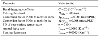
Table 1Key ice-sheet model and climate forcing parameters. Conversion factor units are meters of water equivalent per positive degree day (mwe/PDD).
Here we illustrate the problems derived from this approach and propose a new offline climate forcing method that attempts to better represent the characteristic pattern of millennial-scale climate variability. Ice-core records (e.g., Dansgaard et al., 1993; NGRIP members, 2004) as well as a wide range of coupled climate models (Ganopolski and Rahmstorf, 2001; Menviel et al., 2014; Peltier and Vettoretti, 2014; Banderas et al., 2015; Zhang et al., 2014, 2017) suggest that millennial-scale variability during the LGP was associated with the transition between two different climatic regimes: a stadial and an interstadial state that differ in the location and/or strength of North Atlantic Deep Water (NADW) formation. Here we assume the stadial state represents the background glacial climate at the LGM, with NADW formation south of Iceland, and include the interstadial state as an additional independent snapshot that represents a millennial-scale excitation away from the background state as a result of a northward shift and intensification of NADW formation. A synthetic time-varying temperature climatology is built by combining present-day observations, the simulated LGM anomalies relative to the present, scaled by an orbital-timescale index, and the simulated stadial–interstadial anomalies, scaled by a millennial-timescale index. An important, model-dependent issue is the extent to which the orbital and millennial-scale anomaly fields are well captured, in particular their amplitudes. To account for this, a refinement of the method is proposed consisting in a scaling of both orbital and millennial temperature anomalies. We then compare the effect of the synthetic climatologies built with the three methods on the simulated evolution of NH ice sheets throughout the last glacial cycle.
The paper is organized as follows: in Sect. 2 the ice-sheet model and the three climate forcing methods used are described. In Sect. 3 the results of applying these methods to force the ice-sheet model are shown, and their capability to simulate the evolution of the NH ice sheets during the last glacial cycle is compared. Finally, the main conclusions are summarized in Sect. 4.
2.1 The ice-sheet model description
The model used in this study is the GRISLI ice-sheet model, developed by Ritz et al. (2001). GRISLI has been used in a number of studies in different domains including Antarctica (Ritz et al., 2001; Philippon et al., 2006; Álvarez-Solas et al., 2011a), Greenland (Quiquet et al., 2012, 2013) and glacial NH ice sheets (Peyaud et al., 2007; Álvarez-Solas et al., 2011b, 2013). For this reason and because the focus of our study is the climate forcing used to drive the model, only a brief description is given here; further details about the model can be found in these previous studies.
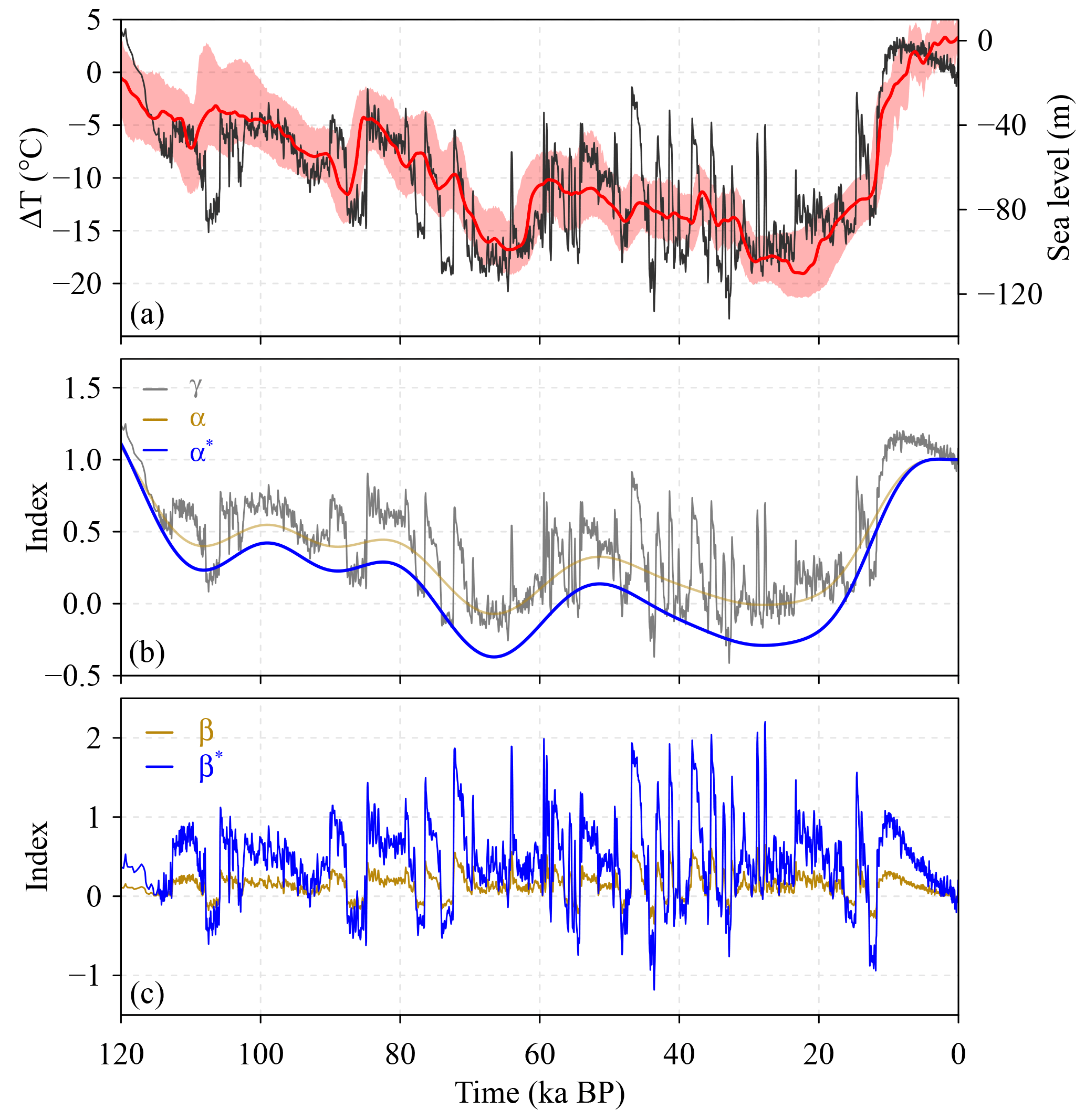
Figure 1Temporal components of the three forcing methods. (a) Sea-level forcing (m) as estimated by Grant et al. (2012). The light red shaded area represents the 95 % confidence level interval of the prescribed sea-level reconstruction. The black curve shows the evolution of temperature anomalies (∘C) relative to the present over Greenland from which the index is derived (Vinther et al., 2009; Kindler et al., 2014). (b) Index used in M1 (γ; gray) together with the orbital components of the indices used in M2 (α; gold) and M3 (α⋆; blue). (c) Millennial components of the index used in M2 (β; gold) and M3 (β⋆; blue).
GRISLI is a hybrid three-dimensional thermomechanical ice-sheet model combining the shallow ice approximation (SIA; Hutter, 1983) for grounded ice and the shallow shelf approximation (SSA; MacAyeal, 1989) for ice shelves and ice streams. In this model configuration, inland ice that is frozen to the bed is treated using SIA dynamics. When the base of the ice sheet becomes temperate (i.e., there is water at the base) or when the ice is floating, then SSA dynamics apply. The basal friction (τb) is calculated as a linear function of the basal velocity (ub) that is proportional to effective pressure (Neff): (see Table 1 to check the exact value of basal dragging coefficient C). GRISLI uses finite differences on a staggered Cartesian grid at a 40 km resolution, corresponding to 224 × 208 grid points for the NH domain, with 21 vertical levels. Initial topographic conditions are provided by present surface and bedrock elevations built from the ETOPO1 dataset (Amante and Eakins, 2009) and ice thickness (Bamber et al., 2001). Boundary conditions include the surface mass balance (SMB) and basal melting. The SMB is given by the sum of accumulation and ablation, both of which are calculated from monthly surface air temperatures (SATs) and monthly total precipitation. As these variables are strongly influenced by topographic effects, GRISLI accounts for changes in elevation at each time step considering a linear atmospheric vertical profile for temperature with different lapse rates in summer and in the annual mean to account for the smaller summer atmospheric vertical stability (Table 1) (Ohmura and Reeh, 1991) and an exponential dependency of precipitation on temperature. Accumulation is calculated by assuming that the fraction of solid precipitation is proportional to the fraction of the year with a mean daily temperature below 2 ∘C. The daily temperature is computed from monthly SATs assuming that the annual temperature cycle follows a cosine function. Ablation is calculated using the positive-degree-day (PDD) method (Reeh, 1989). All PDD parameters are kept constant in all simulations over the entire domain (see Table 1 for the exact parameter values). Note that as indicated by Bauer and Ganopolski (2017), using fixed PDD factors, it is not possible to realistically simulate the glacial evolution of the NH ice sheets in coupled climate–ice-sheet models. The reason being that the increase in CO2 and insolation after the LGM is not efficient enough to satisfactorily simulate the deglaciation when using a PDD approach. Here, and for all the index methods, the deglaciation is explicitly driven by an imposed increase in temperatures; thus, the problem mentioned does not appear. Nevertheless, our goal is not to provide the most realistic simulation, which should include coupling with the climate system, higher resolution and a better representation of surface mass balance processes, but rather to highlight and overcome an important deficiency of current offline methods. Basal melting inland is determined through a recent reconstruction of the present-day geothermal heat flux (Shapiro and Ritzwoller, 2004), while in the ocean it is set to a fixed value of 2 m a−1 in regions where depth is greater than 450 m and fixed at 0 m a−1 in shallower areas to favor the growth of ice sheets during cold periods. Increasing background basal melting values modulates the response of NH ice sheets to millennial-scale forcing (see Supplement). A more detailed analysis of the effect of oceanic changes on NH ice sheets will be addressed in future work.
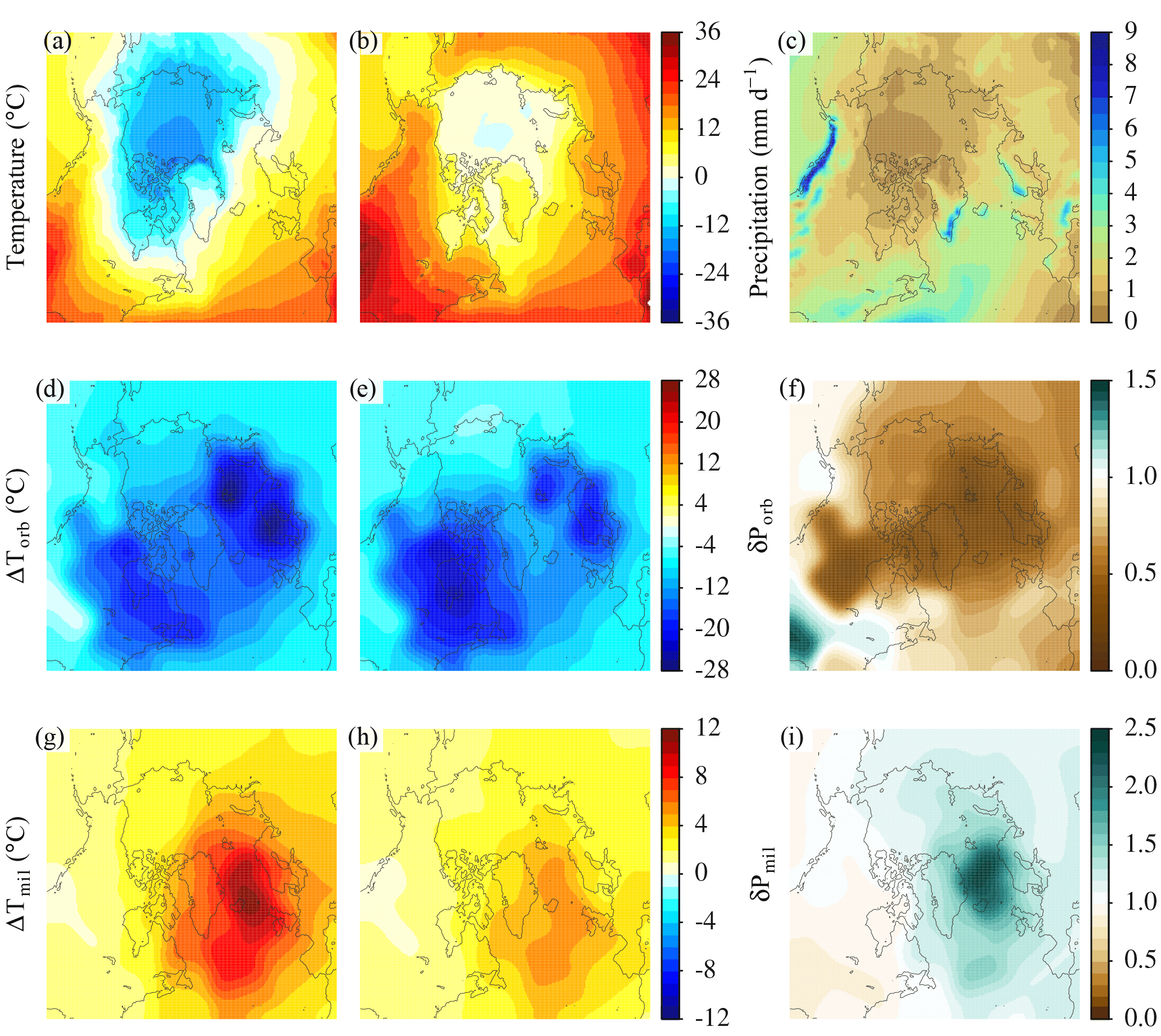
Figure 2Spatial components of the different methods. The reference climate is based on the ERA-INTERIM (1981–2010) reanalysis (Dee et al., 2011) and consists of (a) annual SAT (∘C); (b) summer (JJA) SAT (∘C) and (c) annual precipitation (mm d−1). The orbital component of the spatial forcing comprises the anomalies between the LGM and the present-day climates obtained from the CLIMBER-3α model (Montoya and Levermann, 2008): (d) annual SAT (∘C), (e) summer (JJA) SAT (∘C) and (f) annual precipitation ratio (δPorb = Plgm∕Ppd). Panels (g–i) show the same fields as in (d–f) for the millennial component of the spatial forcing generated from the combination of the Is and the St climatic states simulated by CLIMBER-3α (Banderas et al., 2012, 2015). All variables have been corrected by elevation assuming a linear vertical atmospheric profile (see Sect. 2.1).
2.2 The forcing methods
Synthetic time-varying climatologies are built using three different methods. All three use a perturbative approach as explained above (Sect. 1) by combining the present-day (PD) climatology obtained from observational data with simulated climate snapshots of the last glacial cycle and a time-dependent index derived from proxy records. In all cases the indices used were built based on two recent complementary temperature reconstructions over Greenland (Fig. 1): one from the NGRIP ice-core record for the LGP (Kindler et al., 2014) and another one from several ice-core records for the Holocene (Vinther et al., 2009). Their combination (hereafter, the KV reconstruction) results in a continuous temperature reconstruction over Greenland for the past 120 kyr (Fig. 1a). The present-day climatology (Fig. 2a–c) is taken from the ERA-INTERIM reanalysis (Dee et al., 2011). The climatic snapshots (Fig. 2d–i) are obtained from climate simulations performed with the CLIMBER-3α model (Montoya and Levermann, 2008; Banderas et al., 2015; see Sect. 2.2.1–2.2.3). Due to the relatively low resolution of the atmospheric model (7.5∘ × 22.5∘; latitude × longitude), we perform a two-step interpolation procedure to obtain the forcing fields at the resolution of the ice-sheet model. First, the fields were interpolated conservatively to the ice-sheet model grid. Then, to eliminate artifacts related to model resolution, Gaussian smoothing (also conservative) was applied with a SD of 250 km. Several smoothing windows were tested, with the final choice representing the minimum amount of smoothing necessary to ensure that sharp boundaries between the atmospheric grid cells could not be distinguished on the ice-sheet model grid. The resulting anomalies with respect to the present have been corrected by elevation using the ICE-5G topography (Peltier, 2004). Oceanic temperatures are fixed in all experiments to present-day values to ensure that any ice-sheet changes are exclusively due to the atmospheric forcing. Finally, sea-level variations are prescribed according to the reconstruction by Grant et al. (2012, Fig. 1a). The specific details of each method are described below.
2.2.1 Method 1
The first method (hereafter M1) follows the usual index approach used in many previous studies (Marshall et al., 2000, 2002; Charbit et al., 2002, 2007; Zweck and Huybrechts, 2005). The time-varying temperature and precipitation are given by
where T0 and P0 are the ERA-INTERIM present-day temperature and precipitation climatologies (Fig. 2a–c) and and are the orbital temperature anomaly and precipitation ratio relative to the present day, respectively, obtained from equilibrium simulations for the preindustrial and LGM climates performed with the CLIMBER-3α model (Fig. 2d–f, Montoya and Levermann, 2008). Bold symbols indicate two-dimensional spatial fields. γ is the time index, based on the KV reconstruction, normalized between 0 and 1 for the LGM and the present-day, respectively (Fig. 1a). Thus, the index dictates the timing of both orbital and millennial-scale variability. Note that the γ index can be defined as here (Charbit et al., 2007) or instead as a glacial index (1−γ) that is 0 for the present and 1 for the LGM (e.g., Marshall et al., 2000, 2002; Zweck and Huybrechts, 2005).
2.2.2 Method 2
The second method (M2) is similar to M1 but the temperature and precipitation variability are split into two spectral components, corresponding to orbital and millennial timescales, respectively. The time-varying climatology is now given by
Here ΔTorb and δPorb are as in M1, and and are the millennial temperature anomaly and precipitation ratio, respectively, for the interstadial relative to the stadial state. The stadial mode in our study is represented by the aforementioned LGM climate simulation with CLIMBER-3α (Montoya and Levermann, 2008), while the interstadial mode (Fig. 2g–i) is taken from a transient simulation performed with the same model under glacial climatic conditions but with intensified NADW formation (Banderas et al., 2015). Finally, α and β are two indices that separately modulate the contribution of the orbital and millennial anomalies (Fig. 1). α is obtained after applying a low-pass frequency filter (fc = 1∕18 kyr−1) based on a spectral decomposition to the original KV reconstruction and normalizing the resulting signal to be consistent with the forcing equations (Eqs. 3 and 4); β is obtained following a similar procedure but retaining the high-frequency signal of the KV reconstruction. Thus, . Inspection of Eqs. (1) and (3) shows that the difference between M1 and M2 is just
that is, the difference between the interstadial and the present-day simulated fields, scaled by the millennial-scale β index.

Figure 3(a) Temporal evolution of SAT anomalies (∘C) at the NGRIP site (75.1∘ N, 42.32∘ W) relative to the present day obtained in M1 (gray), M2 (gold) and M3 (blue) as compared to the KV (light green) temperature reconstruction (Vinther et al., 2009; Kindler et al., 2014). (b) Temporal evolution of SAT (∘C) in central Europe from the three methods together with δ18O (‰ Standard Mean Ocean Water, SMOW) variations inferred from stalagmites of northern European Alps (47.38∘ N, 10.15∘ E) as a proxy for air temperature (Moseley et al., 2014). (c) Temporal evolution of precipitation (m a−1) in southwestern North America from the three methods together with δ18O (‰ Vienna Pee Dee Belemnite, VPDB) variations registered in Fort Stanton Cave (33.3∘ N, 105.3∘ W) as a proxy for precipitation (Asmerom et al., 2010). Note the reversed axis in δ18O to facilitate the interpretation of this panel. Vertical colored bars indicate key periods of the past 120 kyr BP.
2.2.3 Method 3
M2 significantly underestimates the amplitudes of millennial-scale fluctuations at the NGRIP ice-core location, as compared to the KV reconstruction (see Fig. 3 and Sect. 3.1). This is a consequence of the attenuated magnitude of the orbital (LGM minus present day) and, particularly, the millennial (interstadial minus stadial) temperature anomalies simulated by the CLIMBER-3α model. To correct for this, method 3 (M3) introduces a refinement with respect to M2 that consists of an adjustment to the time-varying climatology in such a way that the resulting synthetic temperature time series at the NGRIP site exactly matches the KV reconstruction (Fig. 3a). To this end, two additional amplification factors (forb, fmil) are included in the equation that governs the temperature forcing (Eq. 6). Each factor is given by the ratio of the corresponding temperature anomaly component of the KV reconstruction (either orbital, , or millennial, ) to the corresponding temperature anomaly component simulated by the climate model at the NGRIP location (ΔTorb(NGRIP), ΔTmil(NGRIP)), respectively. We thus have
where
and
Here, represents the temperature difference between the PD and the LGM in the orbital component of the KV reconstruction whereas is the maximum temperature amplitude of the millennial-scale component of the KV reconstruction.
are, as in M2, the simulated orbital and millennial-scale temperature anomaly fields of Montoya and Levermann (2008) and Banderas et al. (2015), respectively, evaluated at the NGRIP ice-core location. This tuning to the NGRIP KV reconstruction (Fig. 3) also introduces a scaling of the synthetic temperature amplitudes elsewhere.
Finally, in order to keep the same structure as in the previous methods, the amplification factors are both included within the so-called optimized indices (α⋆, β⋆). Thus,
with
The amplification factors reflect the skill of the climate model to reproduce the characteristic spectral amplitudes of the KV reconstruction at the NGRIP site. Since the model tends to underestimate the KV reconstruction, α⋆ and β⋆ are both found to increase the amplitudes of the orbital and millennial-scale fluctuations, respectively, relative to the original α and β indices (Fig. 1b and c).
3.1 Reconstruction of the NH climate
To evaluate the capability of the different methods to provide a realistic forcing for the ice-sheet model, the resulting synthetic climatologies should be compared against reconstructions. However, continuous, high-resolution NH temperature reconstructions spanning the entire last glacial cycle are scarce. We now compare the performance of each method in regions where proxies are available (see locations in Fig. 4a). Then we discuss the specific features of each method in continental regions that are relevant for ice-sheet growth even though reconstructions are not available.
We first compare the synthetic temperature curves generated in the location of the NGRIP ice core using each method to the KV reconstruction (Fig. 3a). M1 shows an almost perfect agreement with the KV reconstruction. This is due to the fact that the temperature evolution is dictated by γ alone, which comes from the NGRIP record, and that the absolute amplitude, given by the LGM minus present temperature anomaly simulated by the CLIMBER-3α model, at the NGRIP location turns out to be very similar to the glacial–interglacial temperature amplitude (∼ 15 K) of the KV reconstruction (Eq. 1 and Figs. 1 and 2). In contrast, M2 strongly underestimates the amplitude of the KV reconstruction, particularly at millennial timescales. The reason for this is that the amplitude of stadial–interstadial temperature changes simulated by the CLIMBER-3α model at the NGRIP location (∼ 7 K) is smaller than those indicated by the KV reconstruction (up to 16.5 K). In the model the maximum temperature anomaly is actually placed over the Nordic seas, as opposed to off the southeast coast of Greenland, the location where abrupt glacial climate changes are thought to reach their maximum amplitude in terms of temperature (Voelker and workshop participants, 2002). Meanwhile, the exact agreement in the temperature evolution between M3 and the KV reconstruction is predetermined by construction (Sect. 2.2.3).
We further evaluate the three methods through comparison with available temperature and precipitation reconstructions derived from speleothems in central Europe (the Alps) and North America. Time series of SAT in central Europe show an overall qualitative agreement among all three methods (Fig. 3b), which reproduce the phasing and timing of millennial-scale climate variability registered in terrestrial records from the northern European Alps (Moseley et al., 2014). Nevertheless, there are important quantitative differences among the three methods, with M3 showing the SAT changes with the largest amplitudes, followed by M1 and M2 being the smallest ones. Furthermore, the simulated temporal evolution of precipitation in southwestern North America reveals important differences among the methods. In particular, M1 follows the Greenland ice-core temperature evolution with a relatively small amplitude. However, M2 and most notably M3, with a much larger amplitude, show an antiphase relationship with respect to simulated precipitation in M1 (and temperature) on millennial timescales (Fig. 3c). The reason for this lies in the differences that exist within the spatial patterns of orbital and millennial-scale climate variability in this particular region. While the millennial-scale pattern shows slightly wetter conditions during the stadial (i.e., colder climate) as compared to the interstadial (δPmil < 1) in southwestern North America, the orbital spatial pattern exhibits slightly drier conditions at the LGM (i.e., colder climate) as compared to PD conditions (δPorb < 1). Available proxy information indicates that increased precipitation in this area is associated with NH cooling (Asmerom et al., 2010) as opposed to the pervasive NH signal inferred by a wealth of records (Wang et al., 2001; NGRIP members, 2004), which evidences that wetter conditions generally occur during interstadials. Thus, M3 successfully reproduces precipitation variability as interpreted by proxies in this particular region, a result that cannot be achieved by means of the usual index approach.

Figure 4NH ice-sheet configurations at different stages of the last glacial–interglacial period as simulated under M3: (a) present-day ice thickness (km) and (b) present-day ice velocities (km a−1). Panels (c, d) and (e, f) show the same information as (a, b) for the LGM and MIS3 stages, respectively. Red and green contours in panel (c) represent the ICE-5G (Peltier, 2004) and DATED-1 (Hughes et al., 2016) extent of NH ice sheets at the LGM (Peltier, 2004). Colored diamonds (proxy-based information) in panel (a) show the approximate locations of the NGRIP site (light green), Fort Stanton Cave (red) and northern Alps (NALPS) stalagmites. (light blue). Colored dots (proxy-based reconstructions unavailable) show the locations of the two central sites considered at the LIS (purple) and the FIS (yellow).
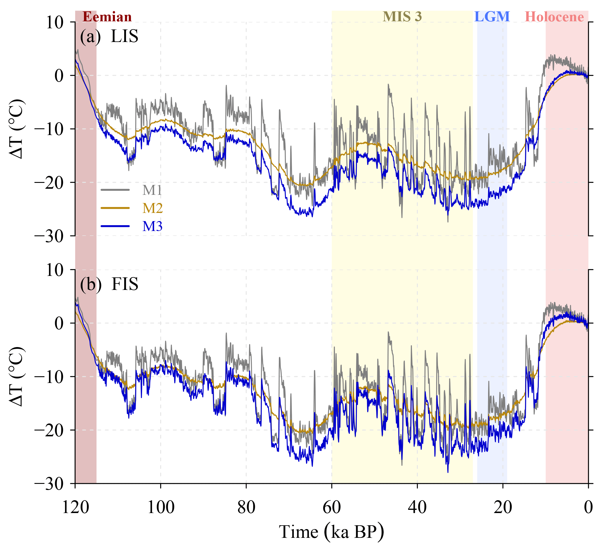
Figure 5Temporal evolution of SAT anomalies (∘C) relative to the present day reconstructed under M1 (gray), M2 (gold) and M3 (blue) scenarios at two central locations of the LIS and the FIS in: (a) North America and (b) Eurasia. Vertical colored bars indicate key periods of the past 120 kyr BP.
The lack of continuous reconstructions in NH continental areas hampers the evaluation of the temperature signal derived from the three methods. Nonetheless, the synthetic temperature time series obtained at two sites, in North America and Fennoscandia, are assessed (Fig. 5). These sites correspond to areas covered by the Laurentide (LIS) and the Fennoscandian (FIS) ice sheets during the LGP, respectively (see locations in Fig. 4a). Several aspects stand out that can be traced back to the structural differences among the methods. First, at orbital timescales, the temperature variations obtained by all methods at both sites show warmer climate conditions in the Eemian (ca. 125 ka BP) with respect to the Holocene (10 ka BP to the present day) and colder temperatures throughout the LGP. By construction, M1 and M2 are identical at these timescales, while in M3 the orbital amplitude is larger, resulting in temperatures 2–5 K colder throughout most of the LGP. Second, at millennial timescales, the amplitudes of the temperature variations obtained with the three methods are very different in both locations. M1 and M2 show the largest and smallest amplitudes, respectively, with differences above 10 K in the most prominent transitions. As previously discussed, M1 and M2 differ only at the millennial scale, by an amount given by Eq. (5). Thus, the difference between these two methods resides in the difference between the orbital and the millennial-scale temperature anomaly fields used in M1 and M2, respectively, scaled by the β index. This boils down to the difference between the present-day and the interstadial temperature fields used in M1 and M2, respectively. These generally result in much larger positive deviations in M1 that, as will be shown below, affect the ice growth. M3 shows variations with intermediate temperature amplitudes between M1 and M2, reflecting the fact that, even with the refined scaling, the amplitude of the millennial temperature anomaly at these sites is much lower than the orbital one (Fig. 2d and g).
Finally, in M1 the amplitude of millennial-scale fluctuations is very similar at both sites as a consequence of the nearly symmetric temperature pattern around Greenland, with two centers of negative values of similar amplitude coinciding with the selected sites (Fig. 2d). In contrast, in M2, and most notably in M3, the differences between the two sites are larger, with larger amplitudes at the FIS than at the LIS site. This is a consequence of the more asymmetric millennial-scale temperature anomaly, characterized by a single center of positive values in the Nordic seas (Fig. 2g).
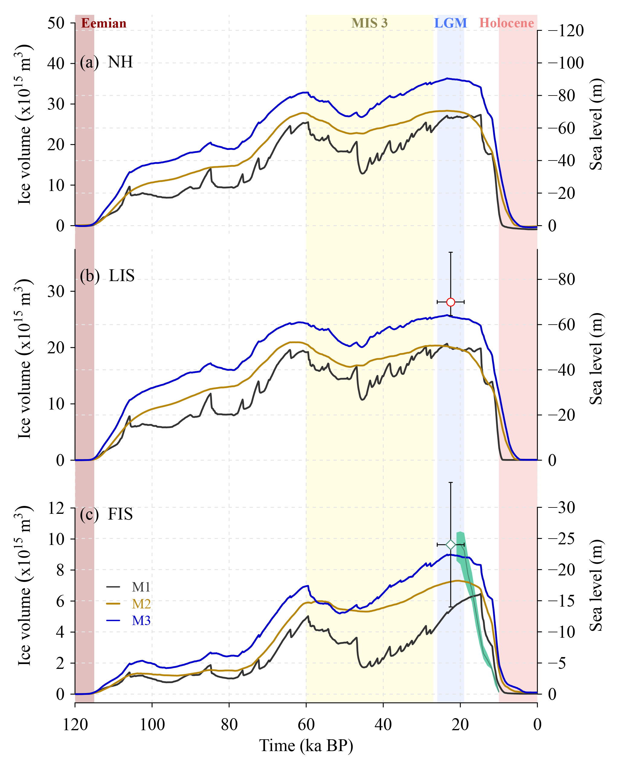
Figure 6Temporal evolution of ice volume (m3) relative to initial conditions simulated in M1 (gray), M2 (gold) and M3 (blue) for (a) the NH domain; (b) the LIS and (c) the FIS. Ice-volume variations have also been expressed in sea-level equivalent units (m). Estimates of the SLE change at the LGM relative to the present for the LIS (red dot; Tarasov et al., 2012) and for the FIS (light green diamond; Hughes et al., 2016) are indicated for comparison in panels (b) and (c), respectively. Vertical error bars represent the range of SLE estimates at the LGM for the LIS and the FIS (Denton and Hughes, 1981; Clark and Mix, 2002; Clark and Tarasov, 2014). Horizontal error bars represent the approximate timing of the LGM (ca. 26.5–19 ka BP; Clark et al., 2009). The temporal evolution of ice volume (m3) for the Eurasian ice sheet from the most-credible DATED-1 reconstruction (light green solid line; Hughes et al., 2016) together with its minimum and maximum lines (shaded area) have also been included in panel (c). Vertical colored bars indicate key periods of the past 120 kyr BP.
3.2 Reconstruction of NH ice sheets
The temporal evolutions of the simulated NH ice sheets that result from imposing the different forcings to the GRISLI model all show the characteristic modulation by orbital climate variability over the last glacial cycle (Fig. 6). Ice volume increases from 120 ka BP throughout the LGP until around 20 ka BP, where it reaches its maximum value, subsequently decreasing throughout the Holocene until the present day.
Important differences are found among the three methods. For all ice sheets, M1 and M3 show the smallest and largest volumes throughout the LGP, respectively; M2 shows intermediate values between the two. As a consequence, of all three methods only M3 agrees with the available LGM minus present SLE reconstructions within their ranges of uncertainties, both for the LIS and the FIS. As mentioned before, by construction, the climates of M1 and M2 are identical at orbital timescales and only differ at millennial timescales. The lower ice volume in M1 relative to M2 is due to the larger amplitude of its millennial-scale fluctuations, resulting from the large amplitude of its orbital spatial component. Indeed, the orbital anomalies used by standard index methods to represent millennial changes are larger than the millennial-scale anomalies. Thus, the forcing and the response are overestimated. Although these sometimes lead to smaller temperatures with respect to the orbital background curve, in general they result in large positive anomalies that, through enhanced ablation, induce a disruption of the growth of large ice sheets in the NH. In contrast, at millennial timescales M2 shows a muted response of ice-volume variations in all ice sheets as a result of the small amplitude of its millennial-scale component. Finally, the higher volumes in M3 compared to M2 are a result of tuning to the lower NGRIP temperature, which results in colder temperatures throughout most of the LGP in the NH (Fig. 5), despite its larger millennial-scale temperature fluctuations. The temperature fluctuations in M3 incorporate both the larger orbital and the smaller millennial amplitude fluctuations compared to M1.
Throughout the LGP, differences in global SLE between the most extreme ice-volume cases, M1 and M3, are generally larger for the LIS, than for the FIS. Regarding the evolution of the LIS, M2 resembles M1 more than M3, but for the evolution of the FIS, M2 resembles M3 more than M1. Around 48 ka BP M1 shows a large ice-volume drop in the FIS that has no counterpart in the LIS (Fig. 6c). M2, in contrast, shows a more gradual evolution. Since the difference between M1 and M2 is exclusively their millennial-scale variability, this would suggest a more important role of their differential millennial-scale variability at the FIS than at the LIS site. However, a simple explanation in terms of local temperature is not possible: at millennial timescales, the temperature difference between M1 and M2 (or M3) is actually smaller for the FIS than for the LIS (Fig. 5). From 60 to 40 ka, the FIS ice volume shows a similar evolution in M1 and M3, with large suborbital (< 19 kyr) ice-volume variability and decreasing trend compared to M2 that can be related to the strong millennial-scale variability after Dansgaard–Oeschger (D–O) event number 17, around 60 ka. The large drop in the FIS ice volume in M1 at 48 ka BP appears to be linked to D–O event number 12, possibly that with the highest amplitude in the whole LGP. However, this D–O event appears both in M1 and M3, and in the latter case it barely has an impact. Thus, a nonlinear response must be invoked to explain the larger impact of millennial-scale variability in M1 in the FIS. Since the magnitudes of the warmings at the LIS and the FIS sites in M1 associated with this D–O are very similar, one possibility is that the lower ice volume of the FIS in M1 around 40 ka leads to a larger reduction in response to the warming of this D–O event through the positive feedbacks between surface elevation and temperature as well as precipitation.
In terms of the extent of NH ice sheets at the LGM, M3 appears to be the best of the three methods, showing the most satisfactory agreement with reconstructions: ICE-5G (Peltier, 2004) for the LIS and DATED-1 (Hughes et al., 2016) for the FIS (Fig. 4c; see also the Supplement). Major deficiencies are found in the southeastern margin of the Scandinavian Ice Sheet (SIS), the southwestern border of the LIS and the northern part of the Cordilleran Ice Sheet (CIS), where the ice extent is underestimated as compared to reconstructions, and northwestern Siberia, where it is overestimated. In M1 and M2, these discrepancies with reconstructions are more evident. Furthermore, in the corridor that separates the CIS and the LIS a significant ice retreat is observed that is absent in M3 (see Supplement).
Finally, the deglaciation shows a different behavior in the three methods. M1 shows a much more abrupt transition into the Holocene, with ice already vanishing by the beginning of this period. This is a consequence of the abrupt temperature evolution in NGRIP that, by construction, in M1 is extrapolated to the rest of the globe, leading to peak temperatures already reached at the beginning of the Holocene and subsequently decreasing. In contrast, M2 and M3 show a smoother temperature evolution at the NH ice-sheet sites (Fig. 5) that also leads to a smoother deglaciation. In all three methods the deglaciation of the FIS is more abrupt than the one suggested by DATED-1 (Fig. 6c). In M3, however, the beginning of the deglaciation (ca. 22 ka BP) is satisfactorily captured. In contrast, the onset of the deglaciation lags behind remarkably in M1, with SLE starting to increase only around 15 ka BP.
We now focus specifically on M3, which provides the best time-varying climatology. The time slices of ice thickness and velocities simulated under M3 provide a consistent picture of the spatial structure of NH ice sheets throughout the LGP (Fig. 4). In particular, the present-day configuration is satisfactorily reconstructed, showing a unique ice sheet over Greenland with regions of intense ice flow predominantly distributed along its southeastern and the northwestern margins (Fig. 4b). Full glacial climatic conditions lead to the growth of two additional vast masses of ice over North America and Eurasia (Figs. 4c and d). On the one hand, the simulated North American ice sheet (NAIS) comprises a merged dome that aggregates the LIS, the Innuitian Ice Sheet (IIS) and the CIS in the western, northern and eastern parts of the continent, respectively. The spatial extent of the NAIS shows good agreement with respect to that estimated in previous studies (e.g., Peltier et al., 2015). The complexity of the NAIS spatial configuration is also reflected in the map of simulated velocities that present two active ice streams in the vicinity of the Hudson Bay and in the area of the Gulf of St. Lawrence in accordance with recent reconstructions (Margold et al., 2015). Meanwhile, the FIS covers the entire Scandinavian region as well as the British Isles and a large fraction of the Barents and the Kara seas as suggested by geological and geomorphological constraints (Hughes et al., 2016; Svendsen et al., 2004). During MIS3, the extension of the NAIS is reduced as compared to the LGM, with an ice-free corridor separating the LIS from the CIS (Figs. 4e and f). The FIS exhibits a decline in terms of volume and extension, particularly in the southwestern sector of the FIS where the British Isles and their surroundings alternate between glaciated and ice-free periods on millennial timescales as a result of abrupt glacial climate variability.
In this study, a new method to force ice-sheet models offline is presented and compared with the more traditional approach. Three different time-varying climatologies are developed for the past 120 kyr following a perturbative approach and applied to an ice-sheet model to evaluate their consequences for the paleo-evolution of ice sheets. In the first case, following the usual approach, temperature anomalies relative to the present are calculated by combining the present-day climatologies, a simulated glacial–interglacial climatic anomaly field and an index derived from ice-core data that includes orbital as well as millennial-scale variability. In the second case, anomalies relative to the present day are decomposed into an orbital and a millennial-scale component. Depending on the frequency either the glacial–interglacial climate anomaly field (orbital variability) or the stadial–interstadial field (millennial) is varied. The third case is a refinement of the second case in which the amplitudes of both orbital and millennial-scale variations are tuned to fit the NGRIP ice-core record. We herein focus essentially on the differences between the traditional and the novel, refined method.
The time series derived from these methods are compared at several locations with the available proxy data: the Greenland ice-core record and reconstructions of temperature and precipitation based on δ18O variations from speleothems located in central Europe and southwestern North America, respectively. By construction, the new method provides perfect agreement with the ice-core record, improving the performance of previous methods. For temperature, the three methods follow a similar evolution, as dictated by the Greenland ice-core record, but the new method shows a larger amplitude. For precipitation, the new method yields a very different time evolution as a result of the spatial millennial-scale anomaly pattern which successfully reproduces the phasing and timing of δ18O variability in southwestern North America on millennial timescales, a result that cannot be achieved by the old method.
Note that offline index methods assume that the temperature variability reconstructed over Greenland is representative of the entire NH, but this does not mean either that the amplitude or the sign is the same in the whole NH. This is actually the case in the usual methods but not in our new method, which is one of the reasons why it represents an improvement. The reason is that the millennial-scale anomaly pattern introduces its own (spatial) scaling. The details of this spatial pattern will depend on the particular climate model used to produce the climate anomaly fields and might well improve with higher complexity and resolution. Most models agree in showing that NH temperature changes coevally with Greenland in response to northward heat transport changes caused by Atlantic meridional overturning circulation (AMOC) variations, the prevailing paradigm to explain abrupt glacial climate changes (e.g., Stouffer et al., 2006), and this is supported by a comprehensive review of spatial coverage (Voelker and workshop participants, 2002), but this is not an assumption of our new index method.
The different climatologies have a large impact on the development of NH ice sheets. In these areas, such as North America and Fennoscandia, traditional methods yield millennial-scale fluctuations of very large amplitude, comparable to those recorded in Greenland. Improving the representation of millennial-scale variability by including a stadial–interstadial anomaly field leads to a strong reduction in the amplitude of millennial-scale temperature fluctuations by more than 10 K in the most prominent transitions. In addition, as a result of the scaling of the orbital temperature anomaly field, the amplitude of orbital variations is enhanced, leading to colder temperatures by about 5 K in most of the LGP. Finally, the traditional method leads to a very similar amplitude of millennial-scale fluctuations over the two main NH landmasses as a consequence of the nearly symmetric temperature pattern around Greenland. In contrast, the improved millennial-scale temperature field leads to the emergence of differences between the temperature evolutions in these areas.
The lack of continuous reconstructions in NH continental areas precludes the evaluation of the temperature time series derived for these regions. However, the fact that in the traditional method the amplitude of temperature variations at sites such as the LIS and the FIS is very similar to those of the Greenland ice-core record strongly suggests that these temperature fluctuations are overestimated. If the mechanisms behind millennial-scale variability are transitions between states of reduced AMOC, with southward-shifted deep water formation (e.g., Sarnthein et al., 1994; Alley et al., 1999; Böhm et al., 2015; Ganopolski and Rahmstorf, 2001; Henry et al., 2016), it is difficult to conceive of a similar temperature amplitude in the center of the LIS or the FIS as in Greenland. Proxy data actually suggest that Greenland is the location where abrupt glacial climate changes reach their maximum amplitude in terms of temperature, decreasing farther south in the NH (Voelker and workshop participants, 2002). In contrast, the temperature fluctuations obtained in the new approach, with amplitudes of 30–50 % of those of the Greenland ice-core record and larger values over the LIS, down- and upstream of the North Atlantic, seem more realistic.
Our results show that the traditional method leads to the lowest ice-volume values throughout the whole LGP. Indeed, millennial-scale climate variability enhances NH ice-volume variability on millennial timescales. This leads to an underestimation of ice volume throughout most of the LGP. Including millennial-scale patterns (in M2) yields an important increase in ice volume in all NH ice sheets but especially in the FIS. Additionally improving the orbital and millennial-scale fields through the scaling is found to increase it further. Note although sea-level records provide essential information to interpret past ice-volume variations, continuous highly resolved sea-level reconstructions are scarce and frequently rely on an insufficient temporal control. In addition, they generally provide inferences on global sea-level changes. This complicates the evaluation of our simulated NH ice-volume time series against the paleorecord. However, the contribution to sea level of individual ice sheets can be assessed at specific time slices such as the LGM, for which reconstructions are actually available. Estimates of the SLE change at the LGM relative to the present Clark and Mix (see the reviews by 2002); Clark and Tarasov (see the reviews by 2014) range between 70 m (Tarasov et al., 2012) and 92 m (Denton and Hughes, 1981) for the LIS and between 14 m (note this case is based on modeling; see Clark and Mix (2002) and references therein) and 34 m (Denton and Hughes, 1981) for the FIS; a recently published reconstruction by Hughes et al. (2016) yields around 23 m. Thus, the traditional method is well below the uncertainty range of ice-volume estimations for the LIS and its lower end for the FIS. In contrast, our new, refined method is closer to the uncertainty range for the LIS and well within it for the FIS. To summarize, even though our method is not perfect, it shows a clear improvement with respect to the usual index method. In particular, the individual (FIS and LIS) and total ice volume and extent of NH ice sheets at the LGM, as well as the timing of the onset of deglaciation, are clearly better captured by our new method. Interestingly, our new approach underestimates ice-volume variations on millennial timescales as indicated by sea-level records. This suggests that either the origin of the latter is not the NH or that processes not represented in our study need to be invoked to account for the important role of millennial-scale climate variability in millennial-scale ice-volume fluctuations. Variation in oceanic conditions, ignored in our study, is a likely candidate.
The climate model used to build the present-day, LGM, and interstadial fields used in this study is an intermediate-complexity model with low spatial (latitude × longitude) resolution (7.5∘ × 22.5∘) (Montoya et al., 2005). Using a more comprehensive and/or higher-resolution model should provide both a more accurate representation of millennial-scale glacial climate variability and a more realistic forcing for the ice-sheet model. Nevertheless, we do not expect this to change our main conclusions. To the extent that orbital and millennial-scale anomaly fields are different, our new forcing method should provide a better representation of the climate of the LGP. We expect this result to be robust against the use of different climate models. The precise temperature and ice-volume evolution could, nevertheless, be model dependent, and this is worth investigating with additional climate models, in particular more comprehensive ones. In the last years a rising number of state-of-the-art climate models have recently shown two different climatic regimes under glacial conditions (Peltier and Vettoretti, 2014; Zhang et al., 2014, 2017). This study opens a new research pathway for these models which could take advantage of our new forcing method to investigate their skill to provide a synthetic reconstruction of the climate variability of the last glacial cycle and apply that to investigate the evolution of NH ice sheets. One recommendation that emerges from our study is that, in case of the unavailability of an interstadial simulated snapshot to force the ice-sheet model, the use of a low-pass-filtered index from the ice-core record should provide a better forcing than the traditional method including the full variability.
In a similar manner, although our ice-sheet model accounts for the surface elevation change feedback on temperature and precipitation, other important climate–ice-sheet feedbacks such as surface albedo changes are not represented. Note, however, that our goal is precisely to improve offline forcing methods, for which most of these feedbacks are inherently absent. It would nevertheless be interesting to investigate this issue further by coupling our ice-sheet model to a regional energy–moisture-balance model where feedbacks such as the ice–albedo feedback, the effect of continentality and the orographic effect on precipitation are better represented.
Finally, the novelty of this work lies in the consideration of an additional climatic pattern associated with millennial-scale climate variability to reconstruct the climate variability of the last glacial–interglacial cycle for the whole NH. Our results reveal that an incorrect representation of the characteristic pattern of millennial-scale climate variability within the climate forcing not only affects NH ice-volume variations at millennial timescales but has consequences for glacial–interglacial ice-volume changes too. Thereby, our new forcing method contributes to clarify the still uncertain role of abrupt glacial climate change in past ice-volume variations, thus shedding light on the evolution of the NH ice sheets. As mentioned above, one aspect that remains to be assessed is the role of the ocean; this should be the focus of future work.
The code used to generate the synthetic climatologies of this study is based on the equations described within the paper. The specific scripts are available from the corresponding author upon request. The variables associated with the three synthetic time-varying climatologies originating in this study are available via this link: http://www.palma-ucm.es/data/ism-forcing/ (last access: 20 May 2018). The evolution of three representative glaciological variables has also been included in the repository as output netCDF files. Additional output variables related to our experiments can be requested from the corresponding author.
The supplement related to this article is available online at: https://doi.org/10.5194/gmd-11-2299-2018-supplement.
RB carried out the simulations, analyzed the results and wrote the paper. All other authors contributed to the design of the simulations, the analysis of the results and the writing of the paper.
The authors declare that they have no conflict of interest.
This work was funded by the Spanish Ministerio de Economía y
Competitividad through project MOCCA (Modelling Abrupt Climate Change, grant
CGL2014-59384-R). Rubén Banderas was funded by a PhD thesis grant of the
Universidad Complutense de Madrid. Alexander Robinson is funded by the Marie
Curie Horizon2020 project CONCLIMA (Grant 703251). Part of the computations
of this work were performed in EOLO, the HPC of Climate Change of the
International Campus of Excellence of Moncloa, funded by MECD and MICINN.
This is a contribution to CEI Moncloa. We would like to thank the two
anonymous reviewers for their suggestions and comments, which have
contributed to improve the paper.
Edited by: Philippe Huybrechts
Reviewed by: Petra Langebroek and one anonymous referee
Alley, R. B., Clark, P. U., Huybrechts, P., and Joughin, I.: The deglaciation of the Northern Hemisphere: a global perspective, Annu. Rev. Earth Pl. Sc., 27, 149–182, https://doi.org/10.1146/annurev.earth.27.1.149, 1999. a
Álvarez-Solas, J., Charbit, S., Ramstein, G., Paillard, D., Dumas, C., Ritz, C., and Roche, D. M.: Millennial-scale oscillations in the Southern Ocean in response to atmospheric CO2 increase, Global Planet. Change, 76, 128–136, 2011a. a
Álvarez-Solas, J., Montoya, M., Ritz, C., Ramstein, G., Charbit, S., Dumas, C., Nisancioglu, K., Dokken, T., and Ganopolski, A.: Heinrich event 1: an example of dynamical ice-sheet reaction to oceanic changes, Clim. Past, 7, 1297–1306, https://doi.org/10.5194/cp-7-1297-2011, 2011b. a
Álvarez-Solas, J., Robinson, A., Montoya, M., and Ritz, C.: Iceberg discharges of the last glacial period driven by oceanic circulation changes, P. Natl. Acad. Sci. USA, 110, 16350–16354, 2013. a
Amante, C. and Eakins, B. W.: ETOPO1 1 Arc-Minute Global Relief Model: Procedures, Data Sources and Analysis, https://doi.org/10.7289/V5C8276M, 2009. a
Asmerom, Y., Polyak, V. J., and Burns, S. J.: Variable winter moisture in the southwestern United States linked to rapid glacial climate shifts, Nat. Geosci., 3, 114–117, 2010. a, b
Bamber, J. L., Layberry, R. L., and Gogineni, S.: A new ice thickness and bed data set for the Greenland ice sheet: 1. Measurement, data reduction, and errors, J. Geophys. Res. Atmos., 106, 33773–33780, 2001. a
Banderas, R., Àlvarez-Solas, J., and Montoya, M.: Role of CO2 and Southern Ocean winds in glacial abrupt climate change, Clim. Past, 8, 1011–1021, https://doi.org/10.5194/cp-8-1011-2012, 2012. a
Banderas, R., Alvarez-Solas, J., Robinson, A., and Montoya, M.: An interhemispheric mechanism for glacial abrupt climate change, Clim. Dynam., 44, 2897–2908, https://doi.org/10.1007/s00382-014-2211-8, 2015. a, b, c, d, e
Banderas, R., Alvarez-Solas, J., Robinson, A., and Montoya, M.: Supplementary data for: A new approach for simulating the paleo-evolution of the Northern Hemisphere ice sheets, available at: http://www.palma-ucm.es/data/ism-forcing/, last access: 20 May, 2018.
Bard, E., Jouannic, C., Hamelin, B., Pirazzoli, P., Arnold, M., Faure, G., and Sumosusastro, P.: Pleistocene sea levels and tectonic uplift based on dating of corals from Sumba Island, Indonesia, Geophys. Res. Lett., 23, 1473–1476, 1996. a
Bauer, E. and Ganopolski, A.: Comparison of surface mass balance of ice sheets simulated by positive-degree-day method and energy balance approach, Clim. Past, 13, 819–832, https://doi.org/10.5194/cp-13-819-2017, 2017. a
Böhm, E., Lippold, J., Gutjahr, M., Frank, M., Blaser, P., Antz, B., Fohlmeister, J., Frank, N., Andersen, M., and Deininger, M.: Strong and deep Atlantic meridional overturning circulation during the last glacial cycle, Nature, 517, 73–76, 2015. a
Bond, G., Broecker, W., Johnsen, S., McManus, J., Labeyrie, L., Jouzel, J., Bonani, G.: Correlations between climate records from North Atlantic sediments and Greenland ice, Nature, 365, 143–147, https://doi.org/10.1038/365143a0, 1993. a
Bonelli, S., Charbit, S., Kageyama, M., Woillez, M.-N., Ramstein, G., Dumas, C., and Quiquet, A.: Investigating the evolution of major Northern Hemisphere ice sheets during the last glacial-interglacial cycle, Clim. Past, 5, 329–345, https://doi.org/10.5194/cp-5-329-2009, 2009. a
Charbit, S., Ritz, C., and Ramstein, G.: Simulations of Northern Hemisphere ice-sheet retreat: sensitivity to physical mechanisms involved during the Last Deglaciation, Quaternary Sci. Rev., 21, 243–265, 2002. a, b
Charbit, S., Ritz, C., Philippon, G., Peyaud, V., and Kageyama, M.: Numerical reconstructions of the Northern Hemisphere ice sheets through the last glacial-interglacial cycle, Clim. Past, 3, 15–37, https://doi.org/10.5194/cp-3-15-2007, 2007. a, b, c
Clark, P. U. and Mix, A. C.: Ice sheets and sea level of the Last Glacial Maximum, Quaternary Sci. Rev., 21, 1–7, 2002. a, b, c, d
Clark, P. U. and Tarasov, L.: Closing the sea level budget at the Last Glacial Maximum, P. Natl. Acad. Sci. USA, 111, 15861–15862, 2014. a, b
Clark, P. U., Dyke, A. S., Shakun, J. D., Carlson, A. E., Clark, J., Wohlfarth, B., Mitrovica, J. X., Hostetler, S. W., and McCabe, A. M.: The last glacial maximum, Science, 325, 710–714, 2009. a
Dansgaard, W., Johnsen, S., Clausen, H., Dahl-Jensen, D., Gundestrup, N., Hammer, C., Hvidberg, C., Steffensen, J., Sveinbjörnsdottr, A., Jouzel, J., and Bond, G.: Evidence for general instability of past climate from a 250-kyr ice-core record, Nature, 364, 218–220, https://doi.org/10.1038/364218a0, 1993. a
Deblonde, G. and Peltier, W.: Simulations of continental ice sheet growth over the last glacial–interglacial cycle: experiments with a one-level seasonal energy balance model including realistic geography, J. Geophys. Res.-Atmos., 96, 9189–9215, 1991. a
Dee, D., Uppala, S., Simmons, A., Berrisford, P., Poli, P., Kobayashi, S., Andrae, U., Balmaseda, M., Balsamo, G., Bauer, P., Bechtold, P., Beljaars, A., van de Berg, L., Bidlot, J., Bormann, N., Delsol, C., Dragani, R., Fuentes, M., Geer, A., Haimberger, L., Healy, S.,Hersbach, H., Hólm, E., Isaksen, L., Kållberg, P., Köhler, M., Matricardi, M., McNally, A., Monge-Sanz, B., Morcrette, J., Park, B., Peubey, C., de Rosnay, P., Tavolato, C., Thépaut, J. and Vitart, F.: The ERA-Interim reanalysis: configuration and performance of the data assimilation system, Q. J. Roy. Meteor. Soc., 137, 553–597, 2011. a, b
Denton, G. H. and Hughes, T. J.: The Arctic ice sheet: an outrageous hypothesis, in: The Last Great Ice Sheets, Wiley, New York, 437–467, 1981. a, b, c
Dyke, A., Andrews, J., Clark, P., England, J., Miller, G., Shaw, J., and Veillette, J.: The Laurentide and Innuitian ice sheets during the last glacial maximum, Quaternary Sci. Rev., 21, 9–31, 2002. a
Ganopolski, A. and Calov, R.: The role of orbital forcing, carbon dioxide and regolith in 100 kyr glacial cycles, Clim. Past, 7, 1415–1425, https://doi.org/10.5194/cp-7-1415-2011, 2011. a
Ganopolski, A. and Rahmstorf, S.: Rapid changes of glacial climate simulated in a coupled climate model, Nature, 409, 153–158, https://doi.org/10.1038/35051500, 2001. a, b
Goelzer, H., Huybrechts, P., Loutre, M.-F., and Fichefet, T.: Impact of ice sheet meltwater fluxes on the climate evolution at the onset of the Last Interglacial, Clim. Past, 12, 1721–1737, https://doi.org/10.5194/cp-12-1721-2016, 2016. a
Grant, K., Rohling, E., Bar-Matthews, M., Ayalon, A., Medina-Elizalde, M., Ramsey, C. B., Satow, C., and Roberts, A.: Rapid coupling between ice volume and polar temperature over the past 150,000 years, Nature, 491, 744–747, 2012. a, b, c
Hays, J. D., Imbrie, J., and Shackleton, N. J.: Variations in the Earth's orbit: pacemaker of the ice ages, Science, 194, 1121–1132, 1976. a
Henry, L., McManus, J. F., Curry, W. B., Roberts, N. L., Piotrowski, A. M., and Keigwin, L. D.: North Atlantic ocean circulation and abrupt climate change during the last glaciation, Science, 353, 470–474, 2016. a
Hughes, A. L., Gyllencreutz, R., Lohne, Ø. S., Mangerud, J., and Svendsen, J. I.: The last Eurasian ice sheets – a chronological database and time-slice reconstruction, DATED-1, Boreas, 45, 1–45, 2016. a, b, c, d, e
Hutter, K.: Theoretical Glaciology: Material Science of Ice and the Mechanics of Glaciers and Ice Sheets, vol. 1, Springer, 1983. a
Imbrie, J., Boyle, E. A., Clemens, S. C., Duffy, A., Howard, W. R., Kukla, G., Kutzbach, J., Martinson, D. G., McIntyre, A., Mix, A. C., Molfino, B., Morley, J. J., Peterson, L. C., Pisias, N. G., Prell, W. L., Raymo, M. E., Shackleton, N. J., and Toggweiler, J. R.: On the structure and origin of major glaciation cycles 1. Linear responses to Milankovitch forcing, Paleoceanography, 7, 701–738, 1992. a
Kindler, P., Guillevic, M., Baumgartner, M., Schwander, J., Landais, A., and Leuenberger, M.: Temperature reconstruction from 10 to 120 kyr b2k from the NGRIP ice core, Clim. Past, 10, 887–902, https://doi.org/10.5194/cp-10-887-2014, 2014. a, b, c
Lambeck, K. and Chappell, J.: Sea level change through the last glacial cycle, Science, 292, 679–686, 2001. a
Lambeck, K., Yokoyama, Y., Johnston, P., and Purcell, A.: Global ice volumes at the Last Glacial Maximum and early Lateglacial, Earth Planet. Sc. Lett., 181, 513–527, 2000. a
Lambeck, K., Yokoyama, Y., and Purcell, T.: Into and out of the Last Glacial Maximum: sea-level change during Oxygen Isotope Stages 3 and 2, Quaternary Sci. Rev., 21, 343–360, 2002. a
Lambeck, K., Rouby, H., Purcell, A., Sun, Y., and Sambridge, M.: Sea level and global ice volumes from the Last Glacial Maximum to the Holocene, P. Natl. Acad. Sci. USA, 111, 15296–15303, 2014. a
Langebroek, P. M., Paul, A., and Schulz, M.: Antarctic ice-sheet response to atmospheric CO2 and insolation in the Middle Miocene, Clim. Past, 5, 633–646, https://doi.org/10.5194/cp-5-633-2009, 2009. a
MacAyeal, D. R.: Large-scale ice flow over a viscous basal sediment: theory and application to ice stream B, Antarctica, J. Geophys. Res.-Sol. Ea., 94, 4071–4087, 1989. a
Margold, M., Stokes, C. R., and Clark, C. D.: Ice streams in the Laurentide Ice Sheet: identification, characteristics and comparison to modern ice sheets, Earth-Sci. Rev., 143, 117–146, 2015. a
Marshall, S. J., Tarasov, L., Clarke, G. K., and Peltier, W. R.: Glaciological reconstruction of the Laurentide Ice Sheet: physical processes and modelling challenges, Can. J. Earth Sci., 37, 769–793, 2000. a, b, c
Marshall, S. J., James, T. S., and Clarke, G. K.: North American ice sheet reconstructions at the Last Glacial Maximum, Quaternary Sci. Rev., 21, 175–192, 2002. a, b, c
Marsiat, I.: Simulation of the Northern Hemisphere continental ice sheets over the last glacial–interglacial cycle: experiments with a latitude–longitude vertically integrated ice sheet model coupled to a zonally averaged climate model, Paleoclimates, 1, 59–98, 1994. a
Menviel, L., Timmermann, A., Friedrich, T., and England, M. H.: Hindcasting the continuum of Dansgaard–Oeschger variability: mechanisms, patterns and timing, Clim. Past, 10, 63–77, https://doi.org/10.5194/cp-10-63-2014, 2014. a
Milne, G. A., Mitrovica, J. X., and Schrag, D. P.: Estimating past continental ice volume from sea-level data, Quaternary Sci. Rev., 21, 361–376, 2002. a
Montoya, M. and Levermann, A.: Surface wind-stress threshold for glacial Atlantic overturning, Geophys. Res. Lett., 35, L03608, https://doi.org/10.1029/2007GL032560, 2008. a, b, c, d, e
Montoya, M., Griesel, A., Levermann, A., Mignot, J., Hofmann, M., Ganopolski, A., and Rahmstorf, S.: The Earth system model of intermediate complexity CLIMBER-3α. Part I: Description and performance for present day conditions, Clim. Dynam., 25, 237–263, https://doi.org/10.1007/s00382-005-0044-1, 2005. a
Moseley, G. E., Spötl, C., Svensson, A., Cheng, H., Brandstätter, S., and Edwards, R. L.: Multi-speleothem record reveals tightly coupled climate between central Europe and Greenland during Marine Isotope Stage 3, Geology, 42, 1043–1046, 2014. a, b
NGRIP members: High-resolution record of Northern Hemisphere climate extending into the last glacial period, Nature, 431, 147–151, 2004. a
Ohmura, A. and Reeh, N.: New precipitation and accumulation maps for Greenland, J. Glaciol., 37, 140–148, 1991. a
Peltier, W.: Global glacial isostasy and the surface of the ice-age Earth- The ICE-5 G(VM 2) model and GRACE, Annu. Rev. Earth Pl. Sc., 32, 111–149, https://doi.org/10.1146/annurev.earth.32.082503.144359, 2004. a, b, c
Peltier, W. and Andrews, J.: Glacial-isostatic adjustment – I. The forward problem, Geophys. J. Int., 46, 605–646, 1976. a
Peltier, W., Argus, D., and Drummond, R.: Space geodesy constrains ice age terminal deglaciation: the global ICE-6G_C (VM5a) model, J. Geophys. Res.-Sol. Ea., 120, 450–487, 2015. a, b
Peltier, W. R. and Marshall, S.: Coupled energy-balance/ice-sheet model simulations of the glacial cycle: a possible connection between terminations and terrigenous dust, J. Geophys. Res.-Atmos., 100, 14269–14289, 1995. a
Peltier, W. R. and Vettoretti, G.: Dansgaard–Oeschger oscillations predicted in a comprehensive model of glacial climate: a “kicked” salt oscillator in the Atlantic, Geophys. Res. Lett., 41, 7306–7313, 2014. a, b
Peyaud, V., Ritz, C., and Krinner, G.: Modelling the Early Weichselian Eurasian Ice Sheets: role of ice shelves and influence of ice-dammed lakes, Clim. Past, 3, 375–386, https://doi.org/10.5194/cp-3-375-2007, 2007. a
Philippon, G., Ramstein, G., Charbit, S., Kageyama, M., Ritz, C., and Dumas, C.: Evolution of the Antarctic ice sheet throughout the last deglaciation: a study with a new coupled climate–north and south hemisphere ice sheet model, Earth Planet. Sc. Lett., 248, 750–758, 2006. a
Quiquet, A., Punge, H. J., Ritz, C., Fettweis, X., Gallée, H., Kageyama, M., Krinner, G., Salas y Mélia, D., and Sjolte, J.: Sensitivity of a Greenland ice sheet model to atmospheric forcing fields, The Cryosphere, 6, 999–1018, https://doi.org/10.5194/tc-6-999-2012, 2012. a
Quiquet, A., Ritz, C., Punge, H. J., and Salas y Mélia, D.: Greenland ice sheet contribution to sea level rise during the last interglacial period: a modelling study driven and constrained by ice core data, Clim. Past, 9, 353–366, https://doi.org/10.5194/cp-9-353-2013, 2013. a
Reeh, N.: Parameterization of melt rate and surface temperature on the Greenland ice sheet, Polarforschung, 59, 113–128, 1989. a
Ritz, C., Rommelaere, V., and Dumas, C.: Modeling the evolution of Antarctic ice sheet over the last 420,000 years: implications for altitude changes in the Vostok region, J. Geophys. Res.-Atmos. (1984–2012), 106, 31943–31964, 2001. a, b
Rohling, E. J., Grant, K., Bolshaw, M., Roberts, A., Siddall, M., Hemleben, C., and Kucera, M.: Antarctic temperature and global sea level closely coupled over the past five glacial cycles, Nat. Geosci., 2, 500–504, 2009. a
Sarnthein, M., Winn, K., Jung, S., Duplessy, J., Labeyrie, L., Erlenkeuser, H., and Ganssen, G.: Changes in east Atlantic deepwater circulation over the last 30,000 years: eight time slice reconstructions, Paleoceanography, 9, 209–267, 1994. a
Shapiro, N. M. and Ritzwoller, M. H.: Inferring surface heat flux distributions guided by a global seismic model: particular application to Antarctica, Earth Planet. Sc. Lett., 223, 213–224, 2004. a
Stouffer, R. J., Yin, J., Gregory, J. M., Dixon, K. W., Spelman, M. J., Hurlin, W., Weaver, A. J., Eby, M., Flato, G. M., Hasumi, H., Hu, A., Jungclaus, J. H., Kamenkovich, I. V., Levermann, A., Montoya, M., Murakami, S., Nawrath, S., Oka, A., Peltier, W. R., Robitaille, D. Y., Sokolov, A. P., Vettoretti, G., and Weber, S. L.: Investigating the causes of the response of the thermohaline circulation to past and future climate changes, J. Climate, 19, 1365–1387, 2006. a
Svendsen, J. I., Alexanderson, H., Astakhov, V. I., Demidov, I., Dowdeswell, J. A., Funder, S., Gataullin, V., Henriksen, M., Hjort, C., Houmark-Nielsen, M., Hubberten, H. W., Ingólfsson, O., Jakobsson, M., Kjær, K. H., Larsen, E., Lokrantz, H., Lunkka, J. P., Lysa, A., Mangerud, J., Matiouchkov, A., Murray, A., Möller, P., Niessen, F., Nikolskaya, O., Polyak, L., Saarnisto, M., Siegert, C., Siegert, M. J., Spielhagen, R. F., and Stein, R. : Late Quaternary ice sheet history of northern Eurasia, Quaternary Sci. Rev., 23, 1229–1271, 2004. a, b
Tarasov, L., Dyke, A. S., Neal, R. M., and Peltier, W. R.: A data-calibrated distribution of deglacial chronologies for the North American ice complex from glaciological modeling, Earth Planet. Sc. Lett., 315, 30–40, 2012. a, b
Vinther, B. M., Buchardt, S. L., Clausen, H. B., Dahl-Jensen, D., Johnsen, S. J., Fisher, D., Koerner, R. M., Raynaud, D., Lipenkov, V., Andersen, K. K., Blunier, T., Rasmussen, S. O., Steffensen, J. P., and Svensson, A. M.: Holocene thinning of the Greenland ice sheet, Nature, 461, 385–388, 2009. a, b, c
Voelker, A., and workshop participants: Global distribution of centennial-scale records for marine isotope stage (MIS) 3: a database, Quaternary Sci. Rev., 21, 1185–1212, https://doi.org/10.1016/S0277-3791(01)00139-1, 2002. a, b, c
Waelbroeck, C., Labeyrie, L., Michel, E., Duplessy, J. C., McManus, J., Lambeck, K., Balbon, E., and Labracherie, M.: Sea-level and deep water temperature changes derived from benthic foraminifera isotopic records, Quaternary Sci. Rev., 21, 295–305, 2002. a
Yokoyama, Y., Lambeck, K., De Deckker, P., Johnston, P., and Fifield, L. K.: Timing of the Last Glacial Maximum from observed sea-level minima, Nature, 406, 713–716, 2000. a
Zhang, X., Lohmann, G., Knorr, G., and Purcell, C.: Abrupt glacial climate shifts controlled by ice sheet changes, Nature, 512, 290–294, 2014. a, b
Zhang, X., Knorr, G., Lohmann, G., and Barker, S.: Abrupt North Atlantic circulation changes in response to gradual CO2 forcing in a glacial climate state, Nat. Geosci., 10, 518–523, https://doi.org/10.1038/ngeo2974, 2017. a, b
Zweck, C. and Huybrechts, P.: Modeling of the northern hemisphere ice sheets during the last glacial cycle and glaciological sensitivity, J. Geophys. Res., 110, D07103, https://doi.org/10.1029/2004JD005489, 2005. a, b, c, d