the Creative Commons Attribution 4.0 License.
the Creative Commons Attribution 4.0 License.
 | 13 Jun 2018
IPA (v1): a framework for agent-based modelling of soil water movement
Andreas H. Schumann
In the last decade, agent-based modelling (ABM) became a popular modelling technique in social sciences, medicine, biology, and ecology. ABM was designed to simulate systems that are highly dynamic and sensitive to small variations in their composition and their state. As hydrological systems, and natural systems in general, often show dynamic and non-linear behaviour, ABM can be an appropriate way to model these systems. Nevertheless, only a few studies have utilized the ABM method for process-based modelling in hydrology. The percolation of water through the unsaturated soil is highly responsive to the current state of the soil system; small variations in composition lead to major changes in the transport system. Hence, we present a new approach for modelling the movement of water through a soil column: autonomous water agents that transport water through the soil while interacting with their environment as well as with other agents under physical laws.
- Article
(1150 KB) - Full-text XML
- BibTeX
- EndNote


Agent-based modelling (ABM) is a relatively new modelling approach or dogma that was born in social sciences to simulate the interactions of autonomous, encapsulated software agents in a predefined environment that form an emergent system through their interactions and their coupled decision-making processes (Macal and North, 2010; Jennings, 2000; North, 2014). Over the years, this technique evolved and came to be applied in various other disciplines like bioinformatics (Centarowicz et al., 2010), land use modelling (Hammam et al., 2004; Crooks et al., 2008), ecological modelling (Kofler et al., 2014), and policymaking (Lempert, 2002). In terms of hydrology, the use cases are mostly restricted to watershed management for coupling natural and social systems (Gunkel, 2005; Bithell and Brasington, 2009; Grashey-Jansen and Timpf, 2010; Troy et al., 2015; Bouziotas and Ertsen, 2017; Mashhadi Ali et al., 2017; O'Connell, 2017). Hydrologic systems are highly dynamic systems which hydrologists try to simulate with a large variety of models from the plot scale to the global scale. Within the modelling community, a manifold of modelling approaches and dogmas exist. Storage models, like Hydrologiska Byråns Vattenbalansavdelning (HBV), separate the catchment into storages that are connected. These connections are expressed as differential equations to describe the alteration of the storages (Lindström et al., 1997). More recently, connectivity models like Connectivity of Runoff Model (CRUM) (Reaney et al., 2007; Kirkby, 2012) were found to better describe the changing interactions among hydrologically active parts of the catchment or the hillslope in contrast to rather stiff models like HBV. The modelling of physical hydrological systems by ABM is sparse in literature, although some approaches were made (Servat, 2000; Folino et al., 2006; Parsons and Fonstad, 2007; Reaney, 2008; Rakotoarisoa et al., 2014; Shao et al., 2015), but they either relied on a less-dynamic predecessor of ABM, the so-called cellular automata, or were restricted to surface flow models. Generally, agent-based models allow a deeper analysis of system behaviour, the relation among dynamic components, and last but not least the ability to model unforeseen dynamics in certain model cases that would otherwise be smoothed out in classic numerical models. Hence, the general advantage of ABM is to test hypotheses of model component interplay in complex situations with unexpected outcomes in which known modelling approaches fail or are hard to parametrize. The unexpected outcome evolves from the multi-agent set-up in which the model outcome is more than the pure addition of all individual decisions but the result of the interplay of decisions. The system behaviour becomes highly complex as soon as agents have to negotiate the solution of a dilemma situation, like in our case an already saturated target area. In contrast to purely data-driven approaches, agent-based models rely on clearly formulated rules that create complex behaviour through large numbers of inter-operating autonomous software units. We see physical process-based agent-based models as appropriate tools for modelling the behaviour of water in the soil matrix in which various processes like chemical alteration and physical processes like the adsorption of water in macropores or the density variation of water through melting-and-freezing processes near permafrost layers are of great hydrologic interest. The modelling of these heterogeneities within the soil, e.g. macropores, is an ideal application for agent-based models as here the interplay of dynamic model components, in this case hydrologic agents, plays a significant role due to changes in the interplay of model components and internal states. Decisions by single agents not only change the model outcome of this very agent but also have a massive influence on the further behaviour of neighbouring agents. These aforementioned processes show a high level of bidirectionality and connectivity, motivating us to set up a framework with a modelling technique that perfectly fits this emergent and dynamic system behaviour.
In our study we wanted to show the ability of dynamic agent-based models to simulate the movement of water through the soil. Therefore, we developed an example model within our Integrated Platform for Agent-based modelling framework (IPA) for agent-based hydrological modelling. IPA follows the instructions for an ABM framework set-up (North, 2014). Our model relies on physical assumptions for percolation speed and distribution of water within the soil matrix. System dynamics are purely based on interactions between hydrologic agents and their environment. With a simple synthetic model set-up we showed that an IPA model compares well with other spatially distributed models, in this case with a model created in the hydrological framework cmf (Kraft et al., 2011). We conducted some virtual experiments with cmf to verify the applicability of IPA in order to overcome the need for a real-data test scenario proving the general applicability of this new modelling approach (Weiler and McDonnell, 2004). Furthermore, we tested the impact of the type of scheduling and the influence of randomness in the choice of the starting position of hydrologic agents after creation. IPA builds upon the agent-based development environment GAMA (Taillandier et al., 2012, 2014) and is published open source on GitHub.
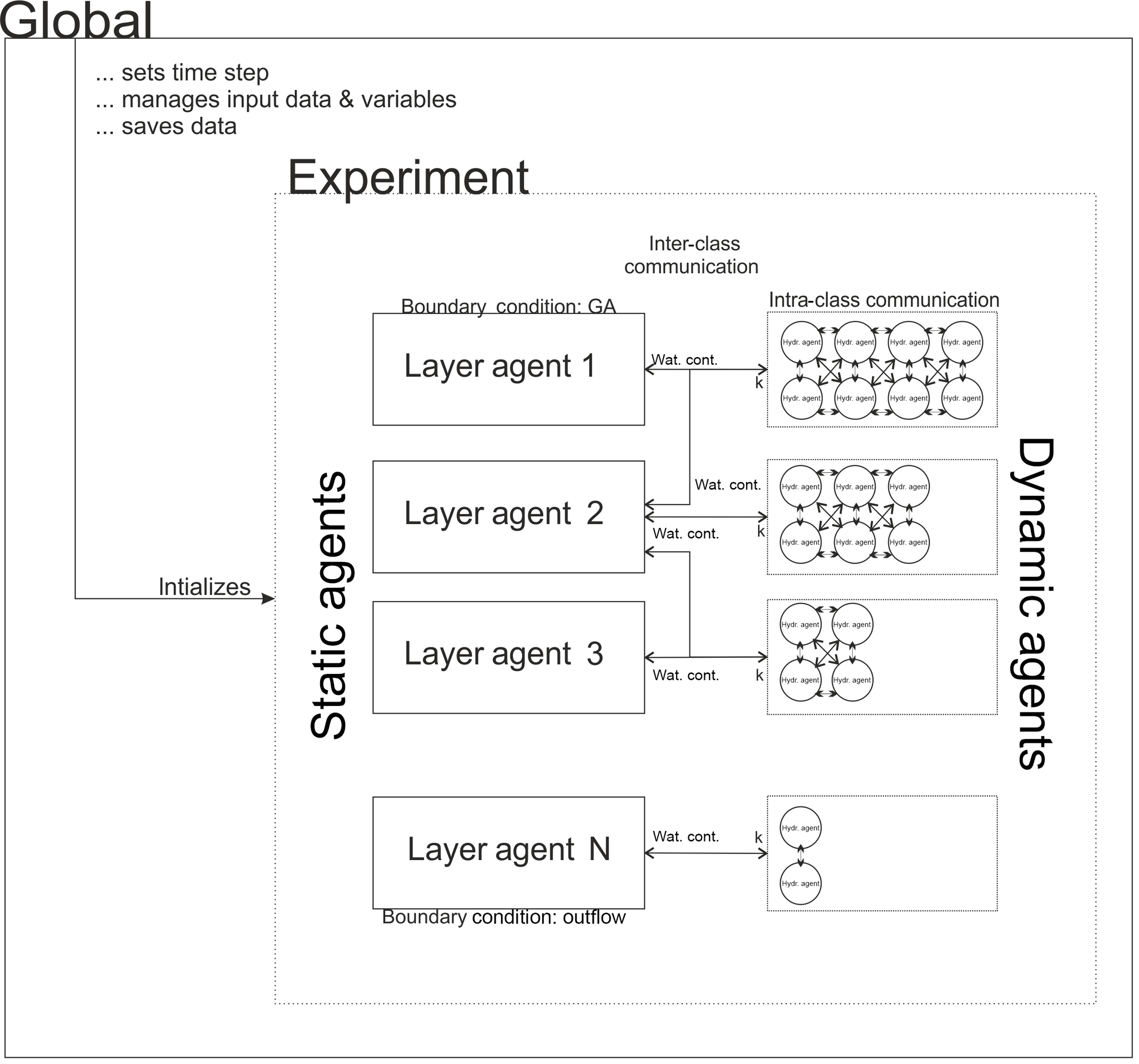
Figure 1Conceptual scheme of IPA showing the global agent, the static layer agents, and the dynamic hydrologic agents that are glued to an experiment. The intra-class communication among hydrologic agents is needed for the pathfinding of the agents, as potential targets for movement might already be occupied. The inter-class communication between hydrologic agents and layer agents shows the information exchange from the dynamic agents to the static agents and vice versa. The bidirectional communication among classes is needed to check boundary conditions like the maximum soil moisture per layer and calculate the potential gradient. Moreover it is used to estimate the velocity k of the hydrologic agent according to their surrounding environment.
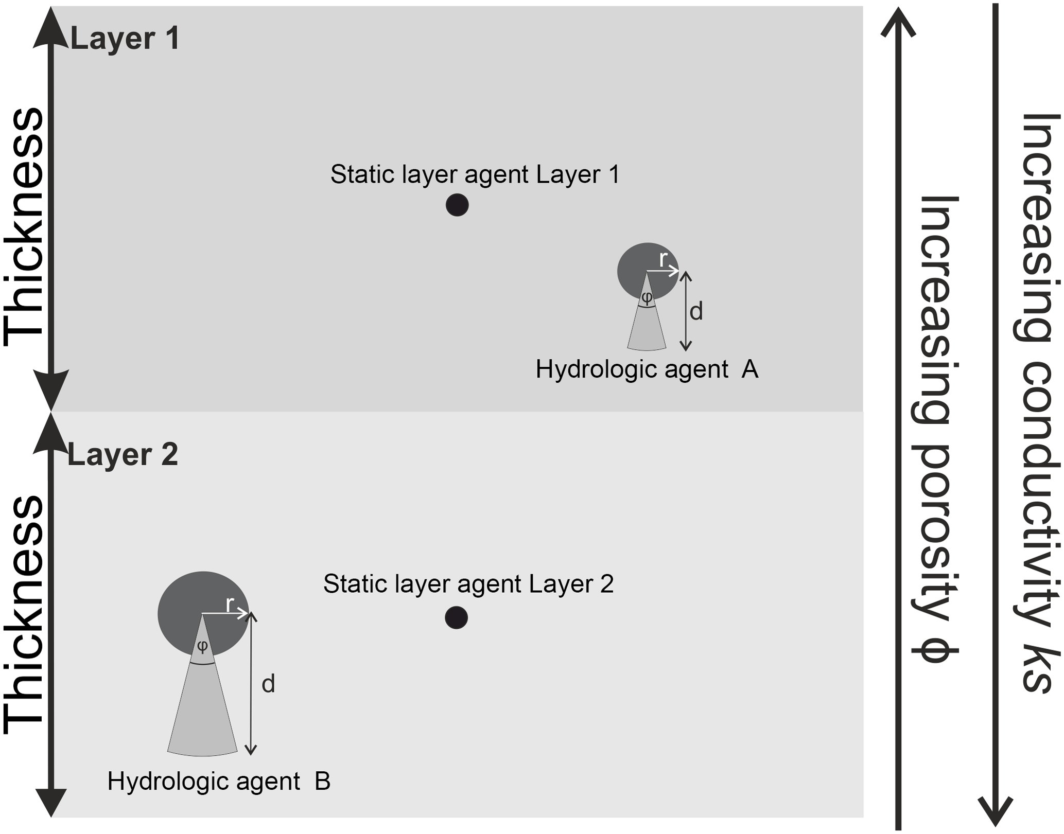
Figure 2IPA scheme with two layers with decreasing porosity per depth and two hydrologic agents.
Following the requirements of an ABM framework, we introduce the class of the dynamic agents, the class of static agents, and the global agent, which controls the modelling experiment as an embracing supervisor (Macal and North, 2010; North, 2014; Fig. 2). In order to set up an agent-based model for soil water modelling, some principal thoughts on the nature of software agents, their interaction with their environment, and eventually the constitution of the model environment must be taken into account (Crooks et al., 2008). Software agents are encapsulated entities with a defined boundary and attributes, which follow rules to fulfil their goal (Macal and North, 2010; Blaschke et al., 2013). Agents interact with their environment through actors and interpret their environment through sensors, whose rules of interaction have to be defined a priori by the modeller (Macal and North, 2010; Hofmann et al., 2015). The environment acts in the form of a defined number of static agents that comprise all hydrologic agents within their spatial and temporal extent. All actions and interactions are coupled and lead to emergent system dynamics: agent A decided to perform action I, which hinders agent B from performing action II but leads agent B to perform action III and eventually force the environmental layer agent to influence agent A's future decision. The IPA framework handles all agent classes, the general composition of the modelled system, and global model behaviour and is designed to manage agents in a dynamic way to allow the composition of large-scale agent-based models through the underlying GAMA architecture in headless mode to save computational time (Taillandier et al., 2012; Boulaire et al., 2015).
In our framework, the global agent manages all static agents (the layers) and dynamic agents (the hydrologic agents). The static agents obtain information from the hydrologic agents, e.g. how much water is already stored within the layer. Conversely, the layers share information on physical properties to the hydrologic agents. They require this information to calculate their movement speed based on the environmental parameters. Through the knowledge about the hydrologic agents inside the layer, the boundary conditions for each layer are checked. In contrast to the aforementioned inter-class communication between layer and agents, the intra-class communication of hydrologic agents is crucial for the decision of movement. In dilemma situations, e.g. in case the target pore space is already covered, the intra-class communication is used to solve that dilemma situation by negotiating the different states of the hydrologic agent (see Fig. 1).
In contrast to classical, equation-based modelling approaches, the number of parameters for tuning is smaller (van Parunak et al., 1998) but the amount of computational time is higher, which results in a demand for parallelized computation either on graphics processing units or on high-performance systems (Wang et al., 2013). Analysis of ABM results is different to analysis of equation-based models. Generally, the pattern-oriented analysis is preferred, especially in the case of spatially distributed ABM (Grimm et al., 2005). In our study, we run GAMA in headless mode to save computational time with 2–4 cores for parallel computing of agent states.
2.1 Dynamic agents: hydrologic agents
2.1.1 Class description of hydrologic agent
Hydrologic agents are carriers of a constant amount of water w that defines their mass (represented as grey circles in Fig. 2). All agents carry the same amount of water, but their spatial extent is different because of changing environmental characteristics. Here, the spatial extent of the hydrologic agents is determined by a circle with radius r that is influenced by the surrounding porosity ΦE. Thus the size of the hydrologic agent may change during its way through the soil column although its mass remains the same due to a change in the porosity. For future applications the density ρ of the carried water is also included (but set to 1).
The influence IhA,L of each hydrologic agent on the static layer agents can be quantified by the area that a hydrologic agent covers of a layer in relation to the complete area of the hydrologic agent (Eq. 2).
where AhA,L is the area of layer L covered by agent hA, and AhA is the area of the hydrologic agent hA. This influence can reach a maximum of 1 if the hydrologic agent covers only one layer, or smaller splits with a sum of 1 per agent, if it covers multiple layers. This influence is used to calculate the saturation of layers and the surrounding porosity ΦE of hydrologic agents in the next time step. The saturation of layers SatL is calculated by the contributed amount of water whA of the agents located within the layer weighted by the influence IhA and the total pore volume of the layer v.
In order to analyse the possible future location of the agent, a cone-shaped viewshed is constructed (light grey cones in Fig. 2). The viewshed has a larger extent than the area of influence, although its length also depends on the radius r. Moreover, the saturated percolation speed of the agent in its environment ks and the chosen model time step Δt determine the viewshed. This can be seen as a tool for numerical integration in the discretized model environment (Servat, 2000), as it shows the maximum distance the agent can travel within the next time step. The cone is constructed with an angle of and the maximum distance d (Eq. 4) and saturated hydraulic conductivity denoted as ks. The calculation of the viewshed is influenced by Darcy's law incorporating the hydraulic conductivity representing the possible step width and the time step of the model. As the agent has a spatial extent, the radius has to be considered as well. The angle φ is a parameter to include the variability in pathfinding due to different grain sizes in the soil structure. As our model set-up is a 1-D soil column and the gradient is limited to one direction, the angle as well is limited to 45∘ in the direction of the gravitational gradient. This angle is chosen because in the 1-D case this angle represents the possible range of direction of movement without a substantially changed gradient. The direction and the speed of movement define the pathfinding algorithm of IPA.
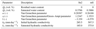
Table 1Physical soil parameters for the Green–Ampt model and van Genuchten model. Source: DBG Arbeitsgruppe Kennwerte des Bodengefüges (2009).
2.1.2 Rule set for hydrologic agents
The hydrologic agent has to decide whether to move or not to move. Once it has decided whether it will move, the direction of movement has to be considered. In our case, the rules of movement are defined by physical laws of soil water movement, which can be seen as a trade-off of vertical forces of gravity ψG and matrix potential ψM that holds water against gravity. These forces are known as the driving potentials. The osmotic potential ψO is neglected, which reduces the decision of each agent for movement to
ψH equalling 0 means no movement down with the potential gradient takes place, whereas ψH>0 leads to capillary rise. ψH<0 results in further deeper percolation of the agent with the speed k of the agent determined by a soil-dependent retention curve (van Genuchten, 1980; DBG Arbeitsgruppe Kennwerte des Bodengefüges, 2009). The speed k is the actual hydraulic conductivity that is higher than the saturated hydraulic conductivity ks. In the case of an infiltration front moving through a wet soil, the matrix potential ψM can also be in the same sign with the gravitational potential ψG. In the case that the future location of the agent at ti+Δt is already occupied, the agent tries to find another route following its gradient of potential. Thus the running order, or schedule of hydrologic agents, is of importance, which we discuss later in detail. If no other route is possible, the particular agent's movement is suspended for this time step, or tick as it is called in ABM. The speed of the movement is given by the k value of the surrounding area, which itself depends on the predominant moisture of the environment, which is calculated using van Genuchten's model (van Genuchten 1980). This model links soil moisture and the predominant potentials ψH, ψM, and ψG with the saturated hydraulic conductivity ks and the hydraulic conductivity k, which is higher under saturated conditions. The physical soil properties used to calculate van Genuchten's model are given in Table 1.
2.2 Static agents: layer agents
2.2.1 Class description of layer agent
As stated before, the layers act as static observing agents that survey all dynamic hydrologic agents that belong to their layer (see Fig. 2). To each static layer agent a corresponding rectangular area is assigned, later on referenced as the layer. Thus the global environment is discretized according to the available data on porosity and layer extents. The total volume of the modelled system is subdivided into a number of single layers. The corresponding soil moisture per layer is calculated by the sum of the internal agents' carried water. As the detection of hydrologic affiliation to a specific layer is vulnerable to numerical artefacts from abrupt changes, the calculated soil moisture is smoothed by a univariate spline with a fifth degree. This spline was found to fit the characteristics of soil water content well, but still needs refinement as we show in the detailed analyses. Each layer controls whether the movement of agents is possible, such that problematic situations, e.g. oversaturation of layers, are avoided. With this the layer is like an internal boundary condition for the decision-making process of the hydrologic agents. The interaction between hydrologic agents and the layer agents is bidirectional: thus, not only corresponding amounts of water carried by hydrologic agents alter layer processes but also this alteration of soil moisture content is coupled with future agents' decision due to the influence of the soil retention curve on speed and direction of movement (Grashey-Jansen and Timpf, 2010).
2.2.2 Rule set for layer agents
Static layer agents have various duties: they create hydrologic agents, monitor the soil moisture, and oversee that all hydrologic agents act within the boundary conditions. For the creation of the hydrologic agents, an infiltration model has to be used. This can be a potential-based agent model, or as well as in this case a Green–Ampt (GA) approach of infiltration leading to the general assumption of a continuous movement of the infiltration front in the matrix. Therefore, the infiltration in the upmost layer represents the upper boundary condition of the model. In this framework an environmental layer can be assigned with a GA infiltration, which offers a fair approximation of GA to compute (Ali et al., 2016). Ali et al. presented an approximation to GA in which F(t) represents the cumulative infiltration, S the sorption parameter defined by Ali et al. (2016), ks the saturated percolation velocity depending on the soil, and t* a dimensionless infiltration time (Eq. 6). The cumulative infiltration F(t) is transformed into an actual infiltration rate f(t), which sets the number of hydrologic agents at a normally distributed random starting position in the upmost layer (Eq. 7). For the calculation of the infiltration into the soil column, the parameters given in Table 1 are used to calculate the GA infiltration in each time step.
The mass of the newly generated agents is fixed to a certain amount which limits the maximum number of agents in the system to be simulated. This knowledge is of importance once IPA is able to run on either graphic card accelerated systems or on parallel computing platforms like cloud-based services because memory allocation and data streaming among processing units become the bottleneck of performance and have to be formalized beforehand (Rybacki et al., 2009; Kofler et al., 2014). In contrast to the upper boundary of the model within the IPA framework, the lower boundary is defined by an outflow rate that relies on the ks value of the lowest layer. Once the centroid of the agent, given as the centre of the circular shaped agent, has left the system, it dies and the carried amount of water accounts as outflow.
In IPA all layers or agents of the environment collect information about processes that take place within their extent and along their boundaries. In order to assign a weight depending on the distance of the hydrologic agents to the centre of the layer, a density kernel approach is applied to assign weights to each agent to smooth results and reduce numerical and graphical artefacts for the integration of all agent movements that are highly variable and are dependent on the simulated situation.
2.3 Scheduling of model actions
Creating agent-based models requires a planned scheme of the running order of processes, actions, and actors (e.g. hydrologic agents and global agents) of the model. Thus, the unifying global agent that combines model parameters, hydrologic agents, and the observing layer agents acts as the controlling unit of the whole model (Macal and North, 2010). This global agent controls the time and acts as an organizing agent because it monitors the initialization of the model (at the beginning of the simulation) and asks hydrologic agents to register their layer belonging. Moreover, the global agent is able to force the observing agents to recalculate their state in terms of their current storage.
2.4 Model framework for comparison: cmf
For comparison purposes, the cmf framework in which a single soil column model was created was used (Kraft et al., 2011). The cmf framework was chosen because it offers an open framework for spatially distributed process-based modelling (like solving the Richard's equation for unsaturated flow). Moreover, the general structure of cmf allows a spatial discretization and spatial modelling and can thus be seen as a possible benchmark for a hydrological ABM framework like IPA.
For our model, a single cmf cell, subdivided into 10 layers with a depth of 10 cm each, was used. The uppermost layer was connected by a GA infiltration process and a constant head of water available for infiltration upon surface. Transportation of water within the cmf soil column was calculated by the Richards equation for unsaturated flow and Darcy's law for saturated flow. The soil retention curve was modelled with the help of the van Genuchten–Mualem model. The outlet of the soil column was defined as a free boundary where water can exfiltrate from the system.
2.5 Model set-up and parametrization of environment
For comparison of the general ability of the usage of IPA for the simulation of soil water movements, a simple synthetic scenario was created. A soil column with a height of 1 m and a width of also 1 m (leading to a complete volume of 1 m3) was used as model set-up. The soil column was divided into 10 single layers with a constant thickness of 10 cm. This column was filled with a homogenous sand soil (mS) with soil parameters given in Table 1. All parameters applied in the van Genuchten model influence the calculation of k by the potential gradient and the saturation of the environment, whereas the GA parameters only affect the upper boundary condition. The chosen time step was 1 h in order to reduce computational time, keeping in mind that a time step this long is vulnerable to numerical integration problems. By the reduction of time step length, fewer steps for the hydrologic agents had to be calculated. All layers were equally pre-filled with soil water, resulting in a layer-specific θ of 20 % of available pore space. Although different in their internal structure, the IPA model and the cmf model (Kraft et al., 2011) shared exactly the same model set-up and parametrization. Infiltration was fed by an initial head of water of 1.0 m at the surface. The number of ticks was set to 90, which means that both models calculated 90 h or 3.75 days of infiltration and soil water movement. The model time was set long enough (3.75 days) to allow a deeper movement of the infiltration front through a set of layers, without the head of water on the surface becoming 0. In both models, the time step is chosen as 1h to increase comparability of results and remains constant in all figures and applications.
2.6 Performance measures
To estimate the quality of IPA representation of the water movement within the soil column, a suitable measure of performance had to be found. Both models deliver time series of their current states, the layer-specific soil moisture θ. Here, we chose to measure the performance of IPA with the r2 value.

Figure 3Comparison of soil moisture development of the upmost three layers with a homogenous soil in the column.
Both models showed no numerical errors over the simulation. The volume error of both models in the end with values of about 1 % are neglectable. With a runtime of 1.1 min on an i5 with 2.2 GHz, 8 GB RAM IPA computed only slightly slower than the numerical cmf model that needed about 30 s on the same set-up. Running IPA in headless mode without graphical output, the computational time was reduced to 48 s. Further reduction of computational time could be archived by an outsourcing of the pathfinding to the graphical computation unit. Comparing both model results, it becomes obvious that results are not exactly the same, yet the dynamics are similar (Fig. 3). The development of soil moisture in the layers follows the same pattern. Saturation reaches a similar level for the first three layers, while the velocity of saturation is different in IPA from the cmf results. Layer 1 does not saturate as fast as in cmf, but movement from Layer 1 to Layer 2 starts earlier in IPA. In cmf, soil water movement from the uppermost layer to the next lower layer starts after approximately 7 h, while the agent-based model triggers movement of hydrologic agents immediately after the first hour of simulation. After 70 h both models show saturation in the first layer, so both models reach the same final stable state. In both models the layers are nearly completely saturated at a soil moisture of about 32.8 %. The transport from Layer 2 to Layer 3 starts in both models 21 h after the beginning of the simulation. Meanwhile, cmf shows a numerically smoother behaviour than IPA, while the general system behaviour is similar as we can see it in the variation in soil moisture in all layers in IPA, although some numerical oscillations in the soil moisture of Layer 2 become visible.
Table 2Statistical parameters from model comparison between cmf and IPA for homogenous soil.
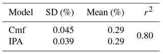
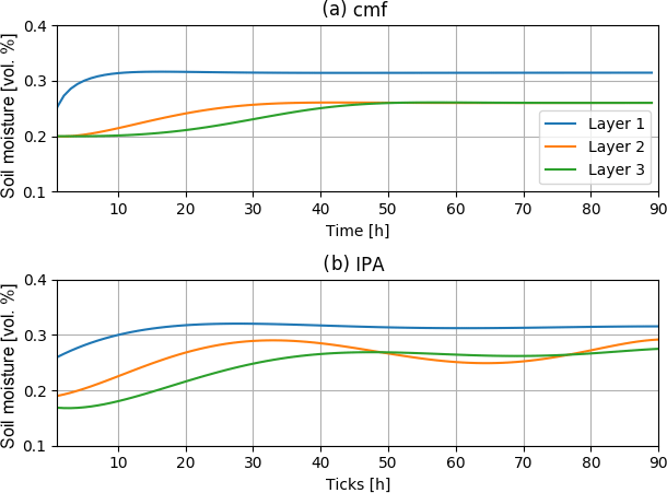
Figure 4Comparison of soil moisture development of the upmost three layers with a transition boundary between Layer 1 and Layer 2.
To express the accordance between IPA and cmf for this run, we calculated the corresponding r2 value. Here the mean r2 value of the upper three layer scores r2=0.80. The standard deviation of both models is slightly different with 0.039 % (cmf) compared to 0.045 % (IPA) while the mean values of soil moisture are the same (Table 2).
4.1 Soil column with heterogeneous soil
As stated before, the synthetic case was extended to a more complex situation of two heterogeneous soil types. In order to show the general ability of IPA to model complex systems, the 1-D soil column was packed with two different soils leading to the problem of a boundary between two different types of soils with different physical properties. The geometry and the discretization of the grid for the cmf model remained the same, but the topmost layer consists of Su2 (a weakly silty sand) instead of mS. Su2 was chosen because although it has different physical characteristics, it is still a relative to the original mS soil with a lower share of sand but a higher share of clay. This change of soil type highly affects the process of infiltration and the transition between Layer 1 and Layer 2. None of the other layers were changed, so the ability of IPA to simulate with its pathfinding algorithm (as introduced in Sect. 2.1.1) and its suspension of movement approach was tested in regard to the added layer transition between Su2 and mS.
Again, both models show a similar, yet slightly different behaviour (Fig. 4). Transport from Layer 1 to Layer 2 starts immediately as does the movement of water between Layer 2 and Layer 3 in IPA. Saturation of Layer 1 in IPA is reached slower than in cmf but the result after 40 h of simulation is a stable system with comparable saturation near full saturation in all layers, although the general IPA behaviour is less smooth than the cmf behaviour. IPA shows slightly higher saturation of about 27 % in contrast to 26 % for Layers 2 and 3 in cmf. For the saturation of the infiltration, Layer 1 shows exactly the same values for both models. The r2 value scores at 0.71, which means a high correlation between the outcomes of both models, even though the dynamics between Layers 2 and 3 are different from those in cmf. This could be related to the dilemma of spatiality in the agent-based model as all hydrologic agents have a certain shape and it is likely that this shape has a significant influence on the model outcome. The slightly higher saturation might be because of the boundary conditions that the global surveying agents have to check to avoid oversaturation.
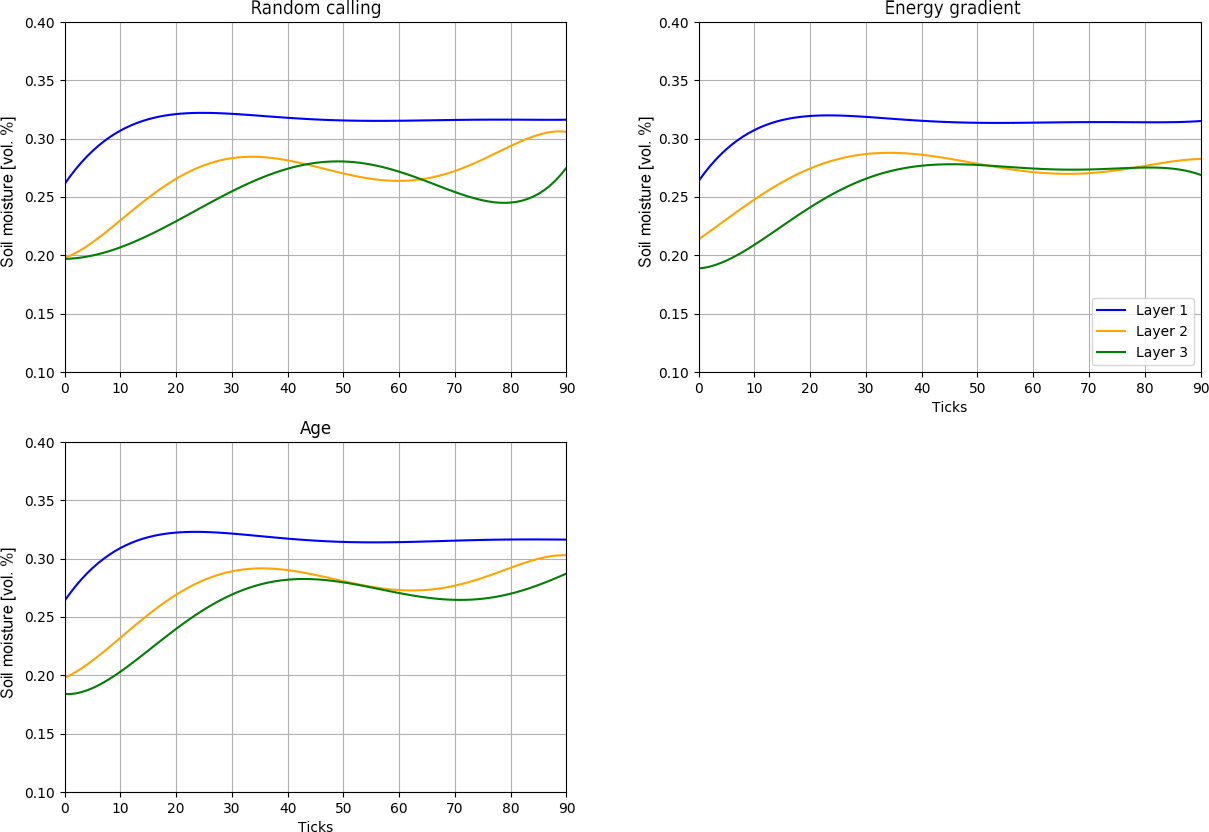
Figure 5Analysis of different scheduling methods for the soil column with two different soils.
4.2 Influence of model scheduling
As mentioned before, scheduling of agent actions is a sensible question in ABM. Here, three different methods for scheduling were implemented:
-
random calling of agents, which calls agents randomly by chance;
-
energy-based scheduling, which allows agents with higher gradients to move first;
-
age-based scheduling, which allows a movement according to the age (either young first or old first).
In order to test the influence of the scheduling approaches on the representation capacity of IPA, we conducted a test with the set-up presented before, with the same duration of simulation and an identical amount of water available for infiltration on the surface (Fig. 5). Random calling of agents is the easiest way to use: for every tick the running order of hydrologic agents is determined randomly. It can be seen that a random scheduling leads to huge smoothing errors because the energy gradient of each agent (the current state of the agent) is not taken into account. Deeper layers show more fluctuations of soil moisture as it can be seen from tick 80 to 90. To overcome this random approach, an energy-based approach was developed: Those agents with the highest energy-gradient are allowed to move first, which results in smoother results with fewer numerical fluctuations. This is the case because the advantage of hydrologic agents with a high potential energy limits conflicts between slow- and fast-moving agents and like for pathfinding issues through a clearly defined regulation, which agents have priority in moving first, trying to get their potentials in balance. Last but not least, we implemented a way to organize the running order by the age of the agents. The age is anticipated by the name because the unique names of all agents are not reused as soon as an agent leaves the system but originate from consecutive numbering during creation. In our test, old water is allowed to move first, so the scheduling is in a decreasing order. This approach has some problems with the distribution of old water because the names of those agents that represent old water are rather similar because they were created during initialization.
Table 3Statistical parameters from model comparison between cmf and IPA for inhomogeneous soil.
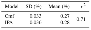
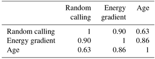
Table 4Correlation coefficient among scheduling methods for Layer 1.
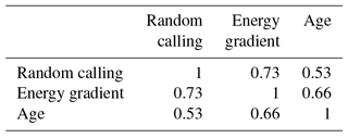
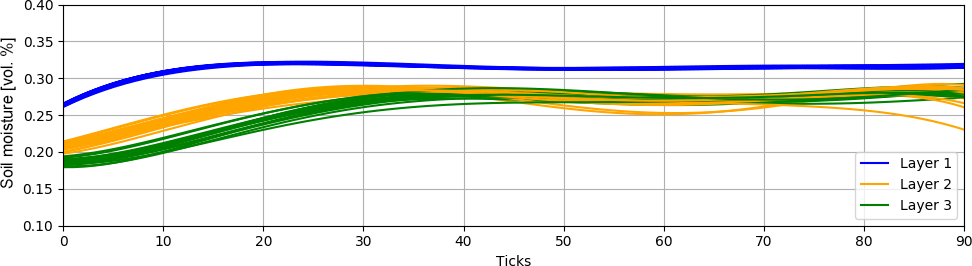
Figure 6Influence of randomly chosen starting point. Calculated with 20 runs and a model set-up with two different soil types.
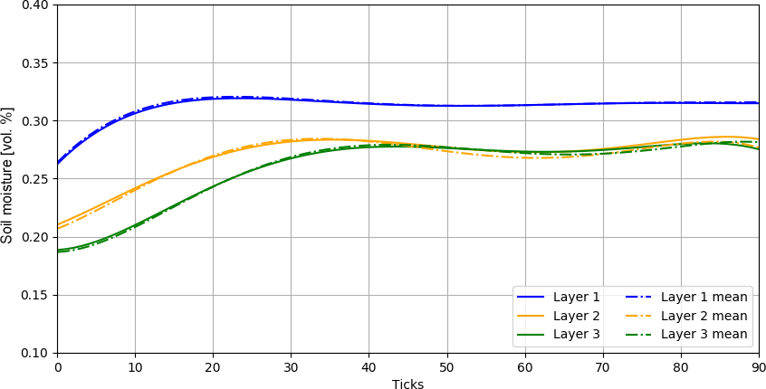
Figure 7Mean resulting soil moisture after 20 runs to reduce effects of randomly chosen starting position.
The correlation coefficients show that all types of scheduling in Layer 1 have less impact than in Layer 2 because all methods do have a high correlation among each other (see Tables 3 and 4). However, correlation coefficients for Layer 2 show that the energy-based approach and the age-based approach have high correlation but struggle less with numerical artefacts like random calling in Layer 2 (Table 5). The soil moisture of the upmost layer is nearly identical in all three cases, which shows once more the dependency of the state of the infiltration-affected layer from the chosen infiltration model. From this analysis, it becomes clear that the energy-based approach seems to be the best fitting approach. These scheduling approaches may be of interest for upcoming application of IPA because technically this scheduling is the major impact factor on the decision-making processes of the hydrologic agents, as one can see in the analysis and can be used for hypothesis testing for the behaviour of water.
Table 5Correlation coefficient among scheduling methods for Layer 2.
4.3 Impact of randomly chosen starting point of hydrologic agents after creation
Another spatial ABM-specific problem is the starting position for the hydrologic agents within the system. The process of infiltration describes the spatial transition of water from the surface to the soil matrix. Therefore, we assume that each hydrologic agent is located with its complete shape in the topmost layer somewhere near the upper boundary. The x coordinates within this layer are chosen randomly around the top of the layer, but always as deep in the soil so that its shape is completely inside the layer. In order to verify our assumptions and to show the impact of different starting positions, we show the influence of the chosen starting position for the same model set up with 20 runs. The starting position was chosen by a random normal distribution with and , where p is varied from 0.1 to 0.9 in 20 steps and is the width of layer, in our case 1m. As one can clearly see, soil moisture in the uppermost layer is only affected by infiltration because calculated soil moisture is nearly constant without any visible influence of the choice of starting position, which makes sense as the hydrologic agent is always located completely within it's the infiltration layer (see Fig. 6). Thus the relevant layers are the deeper Layers 2 and 3. Both show slight variations that look like numerical oscillations, which makes sense as the smoothing affects the calculation of layer soil moisture because the starting position affects the speed and the pathfinding of the hydrologic agents. The maximum gap of soil moisture per layer is at 3 % for Layers 2 and 3 and at 0.5 % for Layer 1 for the 20 runs. However, the variance in soil moisture is visible; thus, a multi-run of n runs should solve the problem and consequently a mean of these n runs should effectively reduce this numerical artefact that was introduced by the random starting point of the agent (Fig. 7).
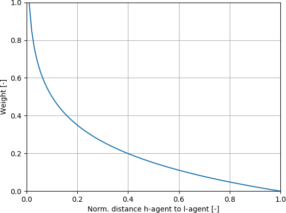
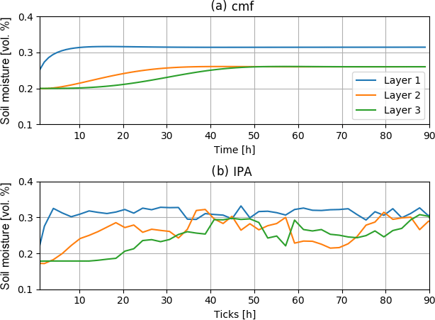
Figure 9Modelled soil moisture without spline smoothing but logarithmic kernel weight assignation.
4.4 Weight assignation: from univariate, fitted spline towards more comprehensible methods
In the first step for each hydrologic agent a weight for influence on the layer was assigned by a fitted univariate spline with 5∘ in order to smooth the numerical artefacts from the calculation of the layer affiliation of hydrologic agents. As univariate splines fit well, but interpretation and transfer to other applications is difficult, we have chosen a density kernel estimator with a simple logarithmic distance function to assign a weight, where wi denotes the weight of the specific hydrologic agent i at distance dl from layer l with which it has a spatial intersection (Eq. 8). This distance is normalized by the maximum possible distance that a hydrologic agent centroid may have with a corresponding layer agent at distance “ld”, which is defined as the maximum of layer depth or the most far away agent that still corresponds to the layer's moisture.
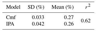
Hydrologic agents lose their influence on the layer moisture with increasing distance from the static layer agent representing the layer centre (see Fig. 8). Implementing a new weight assignation in IPA removed the demand for smoothing the soil moisture per layer. Results for the two-layered synthetic case show that the approach is promising, yet not fully usable because numerical artefacts still appear (especially in Layer 2), where fluctuations around the correct mean soil moisture for this layer occur with the relative strong variation of about 5 % of soil moisture (Fig. 9). Layer 1 is modelled better with fewer fluctuations, the soil moisture rises faster, maximum soil moisture is also modelled correctly and shows only little numerical oscillation. In Layer 1 the layer affiliation of each agent is only relevant during the transition from the layer of origin to the target layer. The overall r2 value is lower with 0.62 than for the spline smoothing, but mean moisture is nearly the same (Table 6). The general interpretation that the model shows similar dynamics is supported by an r2 value that is higher than 0.5, but yet the standard deviation for both modelling approaches is much higher with 0.042 %, with 0.0332 % for cmf or 0.0363 % for spline-based IPA. The kernel-based weighting approach looks promising, as the chosen function is easier to interpret than a univariate spline. However, for future applications, this weight determination has to be improved and might also be part of a study regarding different distance weighting functions and the construction of a method to quickly find the appropriate function.
Table 6Statistical parameters from model comparison between cmf and IPA with kernel-based weight determination.
It was shown that the relatively new modelling approach of agent-based modelling can be used for answering detailed physical-based hydrological questions like the movement of soil water through a soil column. It was shown that an agent-based approach performs well and that its results are comparable to those of a classical Richard's model with Green–Ampt infiltration set up within the cmf framework, which is found to be a suitable environment for modelling complex, spatially distributed hydrological situations with a physically based approach. The comparison revealed some further tasks as problems arise from the agent-based modelling dogma: the smoothing for the calculation of layer moisture needs further refinement, as a spline requires too many degrees of freedom for the task of assignation of weights to each single hydrologic agent (Servat, 2000). A different kernel function will be used (instead of a univariate spline) for better explanatory power of the smoothing process that is needed to compare the highly discretized hydrologic agents with the rather rugged layers in cmf. Moreover, the scheduling needs more refinement, especially in terms of age-based scheduling that still has a high random component, as it became clear during the analysis of different scheduling techniques. The computational time of the IPA model is slightly higher than for the cmf model. The required computation time could be further lowered by running the framework headlessly, which could be a suitable approach for multi-run optimization approaches like Monte Carlo.
In future research on this topic we will take a closer look at possible age distributions for hydrologic agents that represent old water. In this way, we wish to ameliorate the suspension process that hinders a hydrologic agent from moving in favour of another hydrologic agent that blocks the route along the gradient of forces. Thus, the commonly observed phenomenon of residual old water or pushed out old water due to freshwater intrusion can be modelled. In fact, an age-based scheduling also allows finer modelling of hydro-chemical and small-scale pedo-physical processes that occur during the transport of water through the soil matrix than common storage models. Another interesting usage of such a refined age-based scheduling is the residence time of water within a coarse rock glacier in which meltwater is released during rather short melting periods and the water draining from these rock glaciers shows different signatures of age, proving that some water refreezes during the melt and its drain is delayed to later melting periods. Potential applications of spatially distributed hydrological agent-based models are numerous and IPA might be a suitable framework to answer more complex hydrological questions by adding new rule sets. For the modelling of macropore effects on the soil water movement, the principle of agent-based modelling can be interesting: the fastest hydrologic agents wet the surrounding matrix and allow the following water to use the macropore as a shortcut through the matrix until the pore is filled. Through the existence of other hydrologic agents the macropore is filled and travel speed is lowered, which results in an alternative pathfinding through the matrix because the potential gradient allows a dispersion from the pore to the matrix. We will investigate this application of preferential flow in a hydrological model of a coarse rock glacier.
All in all, one can say that IPA and generally agent-based hydrological process models are at their beginning. In times of big data and a plethora of highly resolved data, this new modelling approach can be of use for those questions for which system behaviour can be more easily described with dynamic agent-based models than with stiff storage-based models. Within our examples we showed that the new modelling approach is as good (or as bad) as traditional, storage-based models but offers the variability of extension by rules and different scheduling routines. Even at this stage, an agent-based process model offers a great variability in model design for future research questions as it is able to depict the changing dynamics of model components like in nutrient transport models or complex rock glacier models with changing internal model constellations. The aforementioned variable inner structure of agent-based models extends the modeler's capabilities to describe those systems.
The framework and model are available on GitHub under the following link for general use: https://github.com/HydroMewes/IPA, or under https://doi.org/10.5281/zenodo.1117558 (Mewes, 2018). Example data for soil types mS and Su2 are available in the previously mentioned GitHub repository.
The authors declare that they have no conflict of interest.
We acknowledge support by the DFG Open Access Publication Funds of the
Ruhr-Universität Bochum.
Edited by: Min-Hui
Lo
Reviewed by: two anonymous referees
Ali, S., Islam, A., Mishra, P. K., and Sikka, A. K.: Green-Ampt approximations: A comprehensive analysis, J. Hydrol., 535, 340–355, https://doi.org/10.1016/j.jhydrol.2016.01.065, 2016.
Bithell, M. and Brasington, J.: Coupling agent-based models of subsistence farming with individual-based forest models and dynamic models of water distribution, Environ. Model. Softw., 24, 173–190, https://doi.org/10.1016/j.envsoft.2008.06.016, 2009.
Blaschke, T., Hay, G. J., Kelly, M., Lang, S., Hofmann, P., Addink, E., Queiroz Feito, R., van der Meer, F., van der Werff, H., van Coillie, F., and Tiede, D.: Geographic Object-Based Image Analysis – Towards a new paradigm, ISPRS J. Photogramm., 87, 180–191, https://doi.org/10.1016/j.isprsjprs.2013.09.014, 2013.
Boulaire, F., Utting, M., and Drogemuller, R.: Dynamic agent composition for large-scale agent-based models, in: Complex Adaptive Systems Modeling, 3, 1–23, https://doi.org/10.1186/s40294-015-0007-2, 2015.
Bouziotas, D. and Ertsen, M.: Socio-hydrology from the bottom up: A template for agent-based modeling in irrigation systems, Hydrol. Earth Syst. Sci. Discuss., https://doi.org/10.5194/hess-2017-107, 2017.
Centarowicz, K., Paszyński, M., Pardo, D., Bosse, T., and La Poutré, H.: Agent-based computing, adaptive algorithms and bio computing, ICCS 2010, 1, 1951–1952, https://doi.org/10.1016/j.procs.2010.04.218, 2010.
Crooks, A., Castle, C., and Batty, M.: Key challenges in agent-based modelling for geo-spatial simulation, Comput. Environ. Urban, 32, 417–430, https://doi.org/10.1016/j.compenvurbsys.2008.09.004, 2008.
DBG Arbeitsgruppe Kennwerte des Bodengefüges: Bodenphysikalische Kennwerte und Berechnungsverfahren für die Praxis/Fachgebiete Bodenkunde, Standortkunde und Bodenschutz, Inst. für Ökologie, Bodenökologie und Bodengenese, 40 pp., 2009.
Folino, G., Mendicino, G., Senatore, A., Spezzano, G., and Straface, S.: A model based on cellular automata for the parallel simulation of 3D unsaturated flow, Parallel Comput., 32, 357–376, https://doi.org/10.1016/j.parco.2006.06.003, 2006.
Grashey-Jansen, S. and Timpf, S.: Soil Hydrology of Irrigated Orchards and Agent-Based Simulation of a Soil Dependent Precision Irrigation System, Adv. Sci. Lett., 3, 259–272, https://doi.org/10.1166/asl.2010.1124, 2010.
Grimm, V., Revilla, E., Berger, U., Jeltsch, F., Mooij, W. M., Railsback, S. F., Thulke, H.-H., Weiner, J., Wiegand, T., and DeAngelis, D. L.: Pattern-oriented modeling of agent-based complex systems: lessons from ecology, Science, 310, 987–991, https://doi.org/10.1126/science.1116681, 2005.
Gunkel, A.: The application of multi-agent systems for water resources research–Possibilities and limits, Master Thesis, Institute of Hydrology, Albert-Ludwigs-Universität Freiburg, Freiburg, Germany, 2005.
Hammam, Y., Moore, A., Whigham, P., and Freeman, C.: Irregular vector-agent based simulation for land-use modelling, 16th Annual Colloquium of the Spatial Information Research Centre, Dunedin, New Zealand, 29–30 November 2004.
Hofmann, P., Lettmayer, P., Blaschke, T., Belgiu, M., Wegenkittl, S., Graf, R., Lampoltshammer, T. J., and Andrejchenk, V.: Towards a framework for agent-based image analysis of remote-sensing data, Int. J. Imag. Data Fusion, 6, 115–137, https://doi.org/10.1080/19479832.2015.1015459, 2015.
Jennings, N. R.: On agent-based software engineering, Artif. Intell., 117, 277–296, https://doi.org/10.1016/S0004-3702(99)00107-1, 2000.
Kirkby, M. J.: Do Not Only Connect, in: EGU General Assembly Conference Abstracts, edited by: Abbasi, A. and Giesen, N., vol. 14 (EGU General Assembly Conference Abstracts), p. 3521, 2012.
Kofler, K., Davis, G., and Gesing, S.: SAMPO: an agent-based mosquito point model in OpenCL, Proceedings of the 2014 Symposium on Agent Directed Simulation, Tampa, Florida, Society for Computer Simulation International, 13–16 April 2014, 1–10, 2014.
Kraft, P., Vaché, K. B., Frede, H.-G., and Breuer, L.: CMF: A Hydrological Programming Language Extension For Integrated Catchment Models, Environ. Model. Softw., 26, 828–830, https://doi.org/10.1016/j.envsoft.2010.12.009, 2011.
Lempert, R.: Agent-based modeling as organizational and public policy simulators, P. Natl. Acad. Sci. USA, 99, 7195–7196, https://doi.org/10.1073/pnas.072079399, 2002.
Lindström, G., Johansson, B., Persson, M., Gardelin, M., and Bergström, S.: Development and test of the distributed HBV-96 hydrological model, J. Hydrol., 201, 272–288, https://doi.org/10.1016/S0022-1694(97)00041-3, 1997.
Macal, C. M. and North, M. J.: Tutorial on agent-based modelling and simulation, J. Simul., 4, 151–162, https://doi.org/10.1057/jos.2010.3, 2010.
Mashhadi Ali, A., Shafiee, M. E., and Berglund Zechman, E.: Agent-based modeling to simulate the dynamics of urban water supply: Climate, population growth, and water shortages, Sustain. Cities Soc., 28, 420–434, https://doi.org/10.1016/j.scs.2016.10.001, 2017.
Mewes, B.: IPA model code and examples of soil water models, https://doi.org/10.5281/zenodo.1117558, last access: 7 June 2018.
North, M. J.: A theoretical formalism for analyzing agent-based models, in: Complex Adaptive Systems Modeling, 2, 1–34, https://doi.org/10.1186/2194-3206-2-3, 2014.
O'Connell, E.: Towards Adaptation of Water Resource Systems to Climatic and Socio-Economic Change, Water Resour. Manage., 31, 2965–2984, https://doi.org/10.1007/s11269-017-1734-2, 2017.
Parsons, J. A. and Fonstad, M. A.: A cellular automata model of surface water flow, Hydrol. Process., 21, 2189–2195, https://doi.org/10.1002/hyp.6587, 2007.
Rakotoarisoa, M. M., Fleurant, C., Amiot, A., Ballouche, A., Communal, P. Y., Jadas-Hécart, A., La Jeunesse, I., Landry, D., and Razakamanana, T.: Agents-based modelling for hydrological surface processes on a small watershed (Layon, France), Int. J. Geomatics and Spatial Analysis, 24, 307–333, 2014.
Reaney, S. M.: The use of agent based modelling techniques in hydrology. Determining the spatial and temporal origin of channel flow in semi-arid catchments, Earth Surf. Proc. Land., 33, 317–327, https://doi.org/10.1002/esp.1540, 2008.
Reaney, S. M., Bracken, L. J., and Kirkby, M. J.: Use of the Connectivity of Runoff Model (CRUM) to investigate the influence of storm characteristics on runoff generation and connectivity in semi-arid areas, Hydrol. Proc., 21, 894–906, https://doi.org/10.1002/hyp.6281, 2007.
Rybacki, S., Himmelspach, J., and Uhrmacher, A. M.: Experiments with Single Core, Multi-core, and GPU Based Computation of Cellular Automata, First International Conference on Advances in System Simulation, 2009 (SIMUL '09), Porto, Portugal, 20–25 September 2009, 62–67, 2009.
Servat, D.: Modélisation de dynamiques de flux par agents. Application aux processus de ruisellement, infiltration et érosion, Dissertation, Université Pierre et Marie Curie, Paris, Institut de Recherche pour le developpement, 2000.
Shao, Q., Weatherley, D., Huang, L., and Baumgartl, T.: RunCA: A cellular automata model for simulating surface runoff at different scales, J. Hydrol., 529, 816–829, https://doi.org/10.1016/j.jhydrol.2015.09.003, 2015.
Taillandier, P., Vo, D.-A., Amouroux, E., Drogoul, A.: GAMA: A Simulation Platform That Integrates Geographical Information Data, Agent-Based Modeling and Multi-scale Control, in: Principles and Practice of Multi-Agent Systems, edited by: Desai, N., Liu, A., and Winikoff, M., 13th International Conference, PRIMA 2010, Kolkata, India, 12–15 November, 2010, Springer Berlin Heidelberg, 242–258, 2012.
Taillandier, P., Grignard, A., Gaudou, B., Drogoul, A.: Des données géographiques à la simulation à base d'agents: application de la plate-forme GAMA, Cybergeo, European Journal of Geography, document 671, https://doi.org/10.4000/cybergeo.26263, 2014.
Troy, T. J., Konar, M., Srinivasan, V., and Thompson, S.: Moving sociohydrology forward: a synthesis across studies, Hydrol. Earth Syst. Sci., 19, 3667–3679, https://doi.org/10.5194/hess-19-3667-2015, 2015.
van Genuchten, M. Th.: A closed-form equation for predicting the hydraulic conductivity of unsaturated soils, Soil Sci. Soc. Am. J., 44, 892–898, 1980.
van Parunak, H. D., Savit, R., and Riolo, R. L.: Agent-based modeling vs equation-based modeling, A case study and users' guide, Lect. Notes Comput. Sc., 1534, 10–25, 1998.
Wang, J., Rubin, N., Wu, H., and Yalamanchili, S.: Accelerating Simulation of Agent-Based Models on Heterogeneous Architectures, Sixth Workshop on General-Purpose Computation on Graphics Processing Units (GPGPU-6), Houston, TX, USA, 16 March 2013.
Weiler, M. and McDonnell, J.: Virtual experiments. A new approach for improving process conceptualization in hillslope hydrology, J. Hydrol., 285, 3–18, https://doi.org/10.1016/S0022-1694(03)00271-3, 2004.