the Creative Commons Attribution 4.0 License.
the Creative Commons Attribution 4.0 License.
 | 08 Jun 2018
ORCHIMIC (v1.0), a microbe-mediated model for soil organic matter decomposition
Ye Huang
Bertrand Guenet
Philippe Ciais
Ivan A. Janssens
Jennifer L. Soong
Yilong Wang
Daniel Goll
Evgenia Blagodatskaya
Yuanyuan Huang
The role of soil microorganisms in regulating soil organic matter (SOM) decomposition is of primary importance in the carbon cycle, in particular in the context of global change. Modeling soil microbial community dynamics to simulate its impact on soil gaseous carbon (C) emissions and nitrogen (N) mineralization at large spatial scales is a recent research field with the potential to improve predictions of SOM responses to global climate change. In this study we present a SOM model called ORCHIMIC, which utilizes input data that are consistent with those of global vegetation models. ORCHIMIC simulates the decomposition of SOM by explicitly accounting for enzyme production and distinguishing three different microbial functional groups: fresh organic matter (FOM) specialists, SOM specialists, and generalists, while also implicitly accounting for microbes that do not produce extracellular enzymes, i.e., cheaters. ORCHIMIC and two other organic matter decomposition models, CENTURY (based on first-order kinetics and representative of the structure of most current global soil carbon models) and PRIM (with FOM accelerating the decomposition rate of SOM), were calibrated to reproduce the observed respiration fluxes of FOM and SOM from the incubation experiments of Blagodatskaya et al. (2014). Among the three models, ORCHIMIC was the only one that effectively captured both the temporal dynamics of the respiratory fluxes and the magnitude of the priming effect observed during the incubation experiment. ORCHIMIC also effectively reproduced the temporal dynamics of microbial biomass. We then applied different idealized changes to the model input data, i.e., a 5 K stepwise increase of temperature and/or a doubling of plant litter inputs. Under 5 K warming conditions, ORCHIMIC predicted a 0.002 K−1 decrease in the C use efficiency (defined as the ratio of C allocated to microbial growth to the sum of C allocated to growth and respiration) and a 3 % loss of SOC. Under the double litter input scenario, ORCHIMIC predicted a doubling of microbial biomass, while SOC stock increased by less than 1 % due to the priming effect. This limited increase in SOC stock contrasted with the proportional increase in SOC stock as modeled by the conventional SOC decomposition model (CENTURY), which can not reproduce the priming effect. If temperature increased by 5 K and litter input was doubled, ORCHIMIC predicted almost the same loss of SOC as when only temperature was increased. These tests suggest that the responses of SOC stock to warming and increasing input may differ considerably from those simulated by conventional SOC decomposition models when microbial dynamics are included. The next step is to incorporate the ORCHIMIC model into a global vegetation model to perform simulations for representative sites and future scenarios.
- Article
(1803 KB) - Full-text XML
-
Supplement
(2548 KB) - BibTeX
- EndNote


Soils contain the largest stock of organic carbon (C) in terrestrial ecosystems (MEA, 2005), ranging from 1220 to 2456 Pg C (Batjes, 2014; Jobbágy and Jackson, 2000). Relatively small changes (< 1 %) in this global soil organic carbon (SOC) pool are, therefore, of a similar order of magnitude as anthropogenic CO2 emissions. Warming-induced SOC losses may consequently represent a large feedback to climate change (Jenkinson et al., 1991). Thus, a realistic representation of SOC dynamics in Earth system models is necessary to ensure accurate climate projections, and reduce the uncertainty of SOC stock responses to global climate change; therefore this has been put forward as a research priority (Arora et al., 2013; Friedlingstein, 2015).
In most Earth system models, the decomposition of soil organic matter (SOM) is represented by first-order kinetics (Todd-Brown et al., 2013). The role of microbes during decomposition is not explicitly represented in these models, rather, the decomposition flux, modified by environmental factors, is dependent on the size of the substrate pool. However, these global models fail to accurately reproduce the observed global spatial distribution of SOC (Todd-Brown et al., 2013) even when adjusting parameters (Hararuk et al., 2014), suggesting structural problems in their formulations. One of the underlying reasons might be that microbial community structure and activity are not explicitly represented (Creamer et al., 2015).
Typical SOC models rapidly distinguish decomposing from slowly decomposing plant litter and SOC pools. With first-order kinetics, the decomposition rate of each pool is independent from the other pools, as decomposition rates are decoupled from microbial dynamics. As a result, the priming effect, defined as changes in SOC decomposition rates induced by the addition of fresh, energy-rich organic matter (FOM) (Blagodatskaya and Kuzyakov, 2008), can not be reproduced by these SOC models (Guenet et al., 2016). However, priming effects have been widely observed in laboratory studies, which use different types of soil with different types of FOM added during soil incubation experiments at timescales of less than one day to several hundred days (Fontaine et al., 2003; Kuzyakov and Bol, 2006; Tian et al., 2016), as well as in field experiments (Prévost-Bouré et al., 2010; Subke et al., 2004, 2011; Xiao et al., 2015). The influence of priming on SOC dynamics on long timescales, from years to decades, and at large spatial scales remains uncertain. However, these influences can not be neglected in future SOC stock simulations, considering the projected increase of plant litter inputs to soil in response to the fertilizing effects of elevated CO2, globally increasing nitrogen (N) deposition and lengthening growing seasons (Burke et al., 2017; Qian et al., 2010).
Soil microbial dynamics are believed to be responsible for the priming effect (Kuzyakov et al., 2000). Recently, new models have included the effects of microbial dynamics on SOC decomposition, but not always with an explicit representation of microbial processes (Schimel and Weintraub, 2003; Moorhead and Sinsabaugh, 2006; Lawrence et al., 2009; Wang et al., 2013; Wieder et al., 2014; Kaiser et al., 2014, 2015; He et al., 2015). In those models, SOC decomposition is mediated by soil enzymes released by microorganisms (Allison et al., 2010; Schimel and Weintraub, 2003; Lawrence et al., 2009). Although different groups of microorganisms can produce different enzymes, with large redundancy (Nannipieri et al., 2003), the production of enzymes in models is typically modeled as a fixed fraction of total microbial biomass (Allison et al., 2010; He et al., 2015) or as a fixed fraction of the uptake of C or N (Schimel and Weintraub, 2003; Kaiser et al., 2014, 2015). However, negative priming effects, i.e., reduced SOC decomposition in response to FOM addition, as occasionally observed in soil incubation experiments (Guenet et al., 2012; Hamer and Marschner, 2005; Tian et al., 2016), suggest that the preferential production of enzymes decomposing FOM or an inhibited production of enzymes decomposing SOC is possible. Moreover, it has been reported that enzyme activity can be stimulated by substrate addition and be suppressed by nutrient addition (Allison and Vitousek, 2005). These observations suggest that the production of enzymes is modulated by substrate availability and quality, and not just by microbial uptake or microbial biomass.
Logically, SOC models ignoring microbial dynamics also do not distinguish between active and dormant microbial biomass, thereby neglecting the different physiology of microbes during these two states (Wang et al., 2014). For instance, only active microbes are involved in decomposing SOC (Blagodatskaya and Kuzyakov, 2013) and in producing enzymes (He et al., 2015). However, with 80 % of microbial cells typically being dormant in soils, dormancy is the most common state of microbial communities (Lennon and Jones, 2011). Reactivation of dormant microbes due to the addition of labile substrates is one of the proposed mechanisms explaining the priming effect (Blagodatskaya and Kuzyakov, 2008). Thus, explicitly representing the active fraction of microbial biomass, rather than the entire microbial biomass is a promising avenue to help improve SOC models.
In previous models that explicitly simulate microbial dynamics, enzyme-mediated decomposition rates were modeled using Michaelis–Menten kinetics (Allison et al., 2010), or reverse Michaelis–Menten kinetics (Schimel and Weintraub, 2003; Lawrence et al., 2009). Michaelis–Menten kinetics were also used to model the uptake of C by microbes (Allison et al., 2010). In comparison to these two formulations, first-order accurate equilibrium chemistry approximation (ECA) kinetics performed better than Michaelis–Menten kinetics for a single microbe feeding on multiple substrates or for multiple microbes competing for multiple substrates (Tang and Riley, 2013). ECA kinetics combine the advantages of Michaelis–Menten and reverse Michaelis–Menten kinetics (Tang, 2015), making this formulation more suitable for application in conceptual microbial models.
Nutrient dynamics are often ignored in SOC models (Allison et al., 2010; Wang et al., 2013, 2014; He et al., 2015; Guenet et al., 2016), in particular in the SOC models used with Earth system models (Anav et al., 2013), despite the fact that nutrients can be a rate-limiting for many biological processes in ecosystems (Vitousek and Howarth, 1991). By providing rhizosphere microbes with energy-rich, nutrient-poor exudates, roots may elicit microbial growth, their need for nutrients and subsequently their production of SOC-decomposing enzymes. Thus nutrient availability, especially that of the macroelement nitrogen (N), regulates the priming effect of microbes in response to root exudation (Janssens et al., 2010). Including N dynamics in SOC models is, therefore, also a necessity for accurate projections of future SOC stocks.
In this study, a microbe-driven SOM decomposition model – ORCHIMIC – is described and tested against incubation experiment results. In ORCHIMIC, enzyme production is dynamic and depends on the availability of carbon and nitrogen in FOM and SOM substrates and on a specific pool of available C and N. Three microbial function types (MFTs) – generalists, FOM specialists and SOM specialists – are included, along with an explicit representation of their dormancy; however a fraction of these microbes being cheaters do not invest in producing SOC decomposing enzymes themselves, but profit from the investments of others. ORCHIMIC has been developed with the aim of being incorporated in the ORCHIDEE land biosphere model (Krinner et al., 2005), although its generic input data would allow it to be embedded in any other global land surface model for grid-based simulations.
The ORCHIMIC model is described in Sect. 2 and the two conceptually simpler models – a first-order kinetics model called CENTURY, which was derived from Parton et al. (1987) and constitutes the SOC decomposition module of the ORCHIDEE model (Krinner et al., 2005); and a first-order kinetics model called PRIM, which is a variant of the CENTURY model modified to include interactions between pools to enable the representation of priming of decomposition rates (Guenet et al., 2016) – are described in Sect. 3. The model parameters were calibrated against soil incubation data from Blagodatskaya et al. (2014) (Sect. 4). Different idealized tests of the ORCHIMIC model response including doubling FOM input and/or a stepwise increase in temperature were performed (Sect. 5).
The ORCHIMIC model is zero-dimensional and considers biology and soil physics homogenous within the soil grid to which it is applied. The model simulates C and N dynamics at a daily time step. Inputs of the model are additions of C and N from plant litter or from other sources and plant uptake of N. In return, the model predicts soil carbon and nitrogen pools and respired CO2 fluxes.
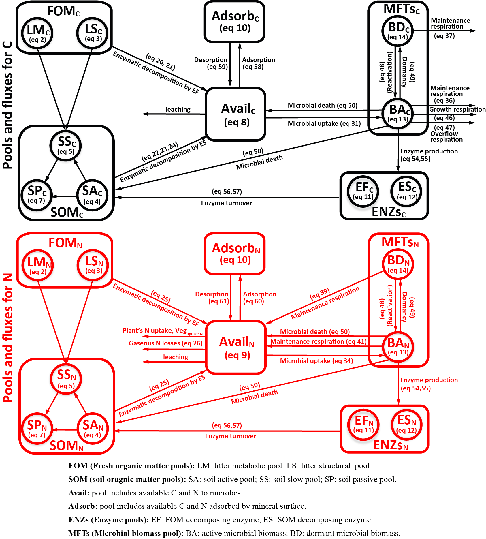
Figure 1Model structure of the ORCHIMIC model. Rectangles and circles represent pools and arrows represent fluxes for Carbon (C; black) and Nitrogen (N; red). The C and N pools are described in Sect. 2.2. Equations describing the dynamics of each pool and the fluxes are shown in brackets in the figure and can be found in more detail in Sect. 2.2 and 2.3. Arrows between the FOM and SOM pools and within the SOM pools represent fluxes due to physicochemical protection by mineral association and microaggregate occlusion. Veguptake,N is uptake of N by plants and is not explicitly simulated by ORCHIMIC.
A total of 11 pools are considered for both C and N (Fig. 1). The two FOM pools are metabolic (LM) and structural (LS) plant litter. The three SOM pools are the active (SA), slow (SS) and passive (SP) pools with short, medium and long turnover times (Parton et al., 1987). SA consists of dead microbes and deactivated enzymes with a short turnover time. SS contains SOM generated during the decomposition of litter and SOM in the SA pool, which is chemically more recalcitrant and/or physically protected with a medium turnover time. SP is a pool of SOM generated during the decomposition of SOM in other pools; it is the most resistant to decomposition and has a long turnover time. The major outgoing C and N fluxes from the substrate pools are the decomposition of the FOM pools by EF enzymes and the SOM pools by ES enzymes. In addition to these major fluxes, there are fluxes from the FOM pools to the SS pool, from SA to both the SS and SP pools and from the SS pool to the SP pool; these fluxes implicitly represent physicochemical protection mechanisms, such as the occlusion of substrates in macroaggregates (Parton et al., 1987).
The available pools (Avail) represent C and N that are directly available to microbes. The Avail pool receives inputs from substrate decomposition, desorption from mineral surfaces, microbial mortality and decay. The Avail pool is depleted by the uptake of C and N by active microbes, adsorption on mineral surfaces and leaching losses. The Adsorb pool represents C and N that are unavailable to microbes because of adsorption by mineral surfaces.
Four MFTs, including SOM specialists, FOM specialists, generalists and cheaters, are explicitly or inexplicitly represented, as described in Sect. 2.1. Each MFT is further divided into active (BA) and dormant (BD) biomass. The outgoing C fluxes from active microbes are growth respiration, maintenance respiration, overflow respiration, dormancy, death and enzyme production. During dormancy, death and enzyme production, corresponding amounts of N are also lost from active microbes. N is furthermore released from active microbes when maintenance respiration is at the cost of their own biomass. Dormant microbes can be reactivated (a flux of C and N from dormant to active microbes) and lose C and release N during maintenance respiration but at a slower rate than active microbes.
The two enzyme pools include enzymes that can decompose either FOM (EF) or SOM (ES). Enzyme pools receive inputs through microbial enzyme production and decline through enzyme turnover. The equations corresponding to each process (shown in Fig. 1) are given in Sect. 2.2, and for fluxes between pools in Sect. 2.3.
2.1 Microbial functional types
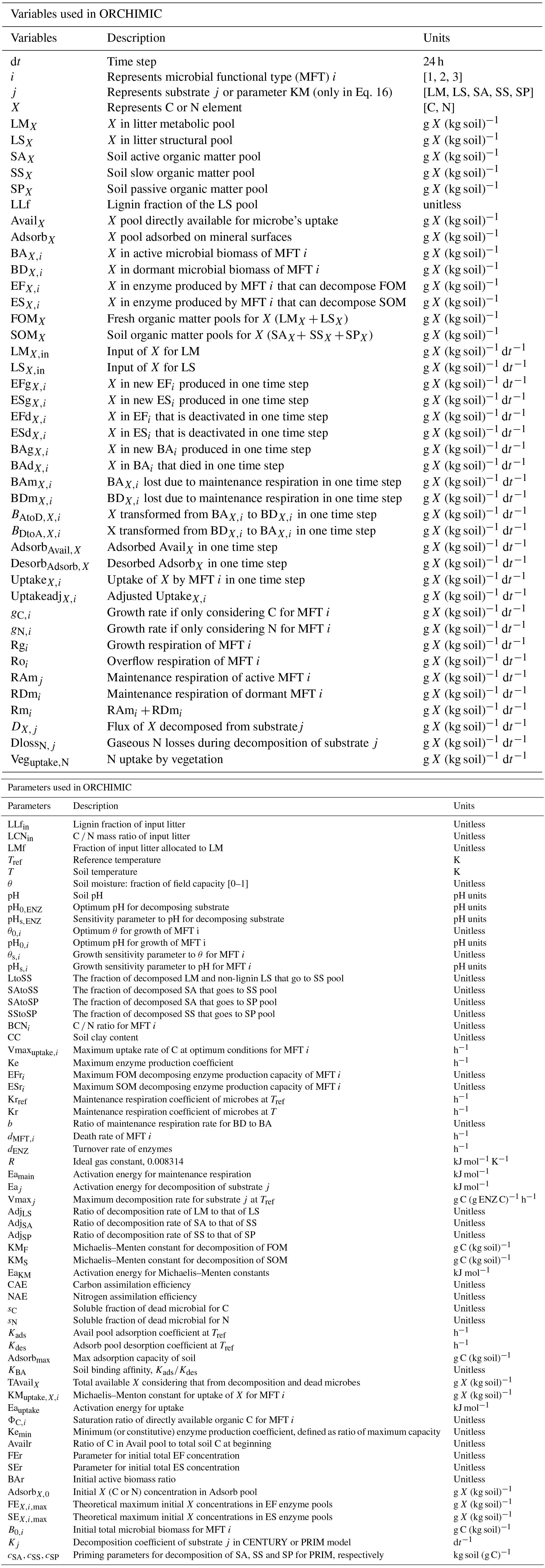
Four MFTs, SOM specialists, FOM specialists, generalists and cheaters, are represented with a set of parameters, including the following: a MFT specific C ∕ N ratio (BCNi) and maximum uptake rate of C (Vmaxuptak,i) for the ith MFT; optimum soil moisture (θ0) and pH (pH0) for microbial uptake; parameters controlling the microbial uptake sensitivities to soil moisture (θs) and pH (pHs); the maximum enzyme production coefficient (Ke); the ability to produce FOM specific enzymes EF (EFri) and SOM specific enzymes ES (ESri); and the dissolvable fraction of dead microbial biomass (sC for C and sN for N) (Table 1). Generalists, SOM specialists and FOM specialists are the three enzyme-producing MFTs that are explicitly considered. The main differences among them are their C ∕ N ratio and their maximum capacity to produce enzymes for decomposing specific pools. The C ∕ N ratios BCNi are set to 4.59 and 8.30 for SOM and FOM specialists, respectively (Mouginot et al., 2014), based on the assumption that SOM decomposers are mainly bacteria and FOM decomposers are mainly fungi (Kaiser et al., 2014). The C ∕ N ratio of generalists is set to 6.12, in-between that of FOM and SOM specialists. The maximum total enzyme production capacities are set to be the same for each MFT. FOM specialists (i=1) can produce more enzymes that decompose FOM (EFr1 : ESr1=0.75 : 0.25); SOM specialists (i=2) can potentially produce more enzymes that decompose SOM (EFr2 : ESr2=0.25 : 0.75); whereas generalists (i=3) can potentially produce both FOM decomposing and SOM decomposing enzymes in equal proportions (EFr3 : ESr3=0.5 : 0.5). However, the real production of the two enzymes depends on availability of substrates and available C.
Cheaters are microbes that do not produce substrate-decomposing enzymes but profit from the enzymes produced by the other MFTs (Allison, 2005; Kaiser et al., 2015). In ORCHIMIC, enzyme production per unit of active microbial biomass decreases with increasing available C availability (see Sect. 2.3.7 for this dynamic enzyme production mechanism). This corresponds to a larger fraction of the microbial biomass behaving as cheaters than when considering that enzyme production per unit of non-cheaters is constant. Because all three MFTs that are explicitly represented can partly act as cheaters, and do so to variable degrees, cheaters are a fourth MFT that is inexplicitly included in the model.
2.2 Carbon and nitrogen pools
2.2.1 Litter pools
The two FOM pools, LM and LS, receive prescribed inputs from plant litter fall. The distribution of FOM carbon between the LM and LS compartments is a prescribed function of the lignin to N ratio of plant material (Eq. 1) following Parton et al. (1987) (see Sect. 2.3.1). The C ∕ N ratio of the LS pool is set to 150 (Parton et al., 1988) and the C ∕ N ratio of the LM pool is variable depending on the C ∕ N ratio of the FOM input (a forcing of ORCHIMIC representing litter quality). The dynamics of the FOM pools are described by the following:
where LMf is the fraction of litter input C allocated to the LM pool; LLfin and LCNin are the respective lignin content and C ∕ N ratio of litter input to the FOM pools; X represents C or N; LMx,in and LSx,in are the litter input partitioned to the LM and LS pools based on LMf and C ∕ N ratio of litter input, respectively; DX,LM and DX,LS are loss of X due to the enzymatic decomposition of LM and LS, respectively (see Sect. 2.3.1).
2.2.2 Soil organic matter pools
The three SOM pools (SA, SS and SP) represent substrates that are decomposed by SOM decomposing enzymes. The SA represents the insoluble part of dead microbes and deactivated enzymes that have a fast turnover time. The dynamics of this pool are described by the following:
where the first term on the right of the equation represents input from non-soluble active microbial biomass mortality summed over all the MFTs; BAdX,i is the input of C or N due to the mortality of MFT i (see Sect. 2.3.6); sX is the proportion of microbial biomass that is soluble; the second term represents the input from enzymes that lost their activity; EFdX,i and ESdX,i are the inputs of C or N due to turnover of EF and ES enzymes, respectively, produced by MFT i (see Sect. 2.3.7); and DX,SA is the loss of C or N due to decomposition of SA (see Sect. 2.3.1).
Regarding the SS pool, there is a flux going from the FOM pool to the SS pool without being processed by microbes. Following the CENTURY model (Parton et al., 1987; Stott et al., 1983), 70 % of lignin in LS is assumed to go to the SS pool without microbial uptake. LtoSS is the fraction of decomposed LM and non-lignin LS that goes into the SS pool. Similarly, there is also a flux from the SA pool to the SS pool that represents non-biological SOM protection processes, such as physical protection (Von Lützow et al., 2008). The dynamics of the SS pool are given by
In the above equation the first term represents the input of X (C or N) from the LM pool without microbial processing; the second and third terms represent input from the non-lignin part and the lignin part of the LS pool, respectively; the fourth term represents input from the SA pool; LLf is the lignin fraction of the LS pool; DX,SS is the loss of C or N from the decomposition of the SS pool (see Sect. 2.3.1); and SAtoSS is the fraction of decomposed SA becoming physically or chemically protected and added to the SS pool, as modified by the soil clay content (CC) (Parton et al., 1987):
The SP pool is more resistant to decomposition than the SS pool. It receives fluxes from the SA and SS pools and its dynamics are described as follows:
where the first and second terms represent input from the SA and SS pools, respectively; SAtoSP = 0.004 and SStoSP = 0.03 are the respective fractions of decomposed SA and SS that go into the SP pool (Parton et al., 1987); and DX,SP is the loss of C or N due to decomposition (see Sect. 2.3.1).
2.2.3 Pools of C and N available for microbial and plant uptake, and gaseous N loss
The available C and N pool (Avail in Fig. 1) represents C and N directly available for microbial uptake. It receives C and N decomposed from FOM and SOM pools, the soluble part of dead microbes (Schimel and Weintraub, 2003; Kaiser et al., 2014) and C and N desorbed from mineral surfaces. C and N from this pool can also be taken up by microbes or adsorbed onto mineral surfaces. N released from microbial biomass after maintenance respiration by dormant and active microbes (only when C uptake is not sufficient) is also assumed to be a input source for the Avail pool. In addition, uptake of N by plant roots (a forcing of ORCHIMIC in the case of coupling with a vegetation model) and loss of C and N due to leaching are modeled as fluxes removed from this pool. Gaseous N loss due to nitrification and denitrification (see Eq. 26 in Sect. 2.3.1) is considered as a decreased input from substrate decomposition. The dynamics of the Avail pool are described by Eqs. (8) and (9) for C and N, respectively.
where UptakeadjC,i is C taken up by MFT i (see Sect. 2.3.2); DesorbAdsorb,C and DesorbAdsorb,N are the fluxes of C and N desorbed from mineral surface, respectively (see Sect. 2.3.8); AdsorbAvail,C and AdsorbAvail,N are C and N absorbed by mineral surface, respectively (see Sect. 2.3.8); DlossN,j is the gaseous N loss; BAgN,i is N assimilated by MFT i (see Sect. 2.3.4); BAmN,i and BDmN,i are N released from the maintenance respiration of active and dormant biomass for MFT i to the AvailN pool, respectively (see Sect. 2.3.3); Veguptake,N is N taken up by plants, a boundary condition of the model; and leachingC and leachingN are the respective losses of C and N due to leaching.
2.2.4 Adsorbed C and N on mineral surfaces
The C and N in the Avail pool can be reversibly adsorbed (Adsorb pool in Fig. 1) and rendered unavailable to microbes and plants (for N). The dynamics of the Adsorb pool are given by
where the first term is the C or N adsorbed onto mineral surface and the second term is the C or N desorbed from mineral surface (see Sect. 2.3.8).
2.2.5 Enzymes pools
We distinguish between two types of enzymes (EF and ES), which catalyze the decomposition of FOM and SOM, respectively. Each MFT produces enzymes according to their specialization. The turnover rate of both types of enzymes is assumed to be the same. The dynamics of the FOM and SOM decomposing enzyme pools are described by the following:
where EFgX,i and ESgX,i are the respective production rates of enzymes EF and ES by MFT i, with i=1 for FOM specialists, i=2 for FOM specialists and i=3 for generalists (see Sect. 2.3.7). EFdX,i and ESdX,i are the turnover rates of the enzymes EF and ES, respectively, produced by MFT i (see Sect. 2.3.7).
2.2.6 Active and dormant microbial biomass pools
In ORCHIMIC, each MFT can be active or dormant and can switch from one state to the other depending on environmental conditions. When active, the mass of each MFT is defined by the balance between their growth, death, production of enzymes, maintenance and growth respiration and exchange of mass with dormant biomass (BD). If the uptake of C can not meet the need for maintenance respiration, the active mass of a MFT will respire part of its biomass as CO2. When microbial biomass becomes dormant, its carbon can be reactivated or respired through maintenance respiration. When respiration is at the cost of their biomass, a corresponding amount of N is assumed to be lost from dormant microbial biomass and goes to the Avail pool so that the stoichiometry of the dormant microbes remains unchanged. The dynamics for active and dormant microbes are described by the following:
where BAgX,i is the increase of BAX due to growth for MFT i (see Sect. 2.3.4); is the X in microbes transformed from dormant state to active state for MFT i; is the X in microbes transformed from active state to dormant state for MFT i (see Sect. 2.3.5); BAdX,i is the loss of X due to death of active biomass of MFT i; and BAmX,i and BDmX,i are the loss of X in active biomass and dormant biomass, respectively, due to maintenance respiration of MFT i.
2.3 Modeling the processes controlling fluxes between pools
2.3.1 Organic matter decomposition
The substrate used by microorganisms includes FOM and SOM. The FOM and SOM pools are decomposed by enzymes EF and enzymes ES, respectively. The decomposition process is modeled using a combination of Arrhenius and Michaelis–Menten equations (Allison et al., 2010), with different Vmax values for each substrate pool and different Michaelis–Menten constants (KM) for FOM and SOM. To avoid unrealistic decomposition rates when enzyme concentrations are high, an enzyme-dependent term was added in the denominator (ECA kinetics). Vmax values are considered to be sensitive to temperature and modeled using an Arrhenius equation (Eq. 16), with higher activation energy (Ea) for more recalcitrant substrates (Allison et al., 2010). KM is also considered to be sensitive to temperature (Allison et al., 2010; Wang et al., 2013) and the dependency of KM on temperature is modeled using an Arrhenius equation with an activation energy (EaKM) of 30 kJ mol−1 (Davidson and Janssens, 2006) (Eq. 16). All decomposition functions are modulated by soil moisture (θ) and pH. The decomposition function of LS is further modified by its lignin content (Parton et al., 1987). The decomposition function of SA is further modified by soil clay content (CC) (Parton et al., 1987). The functions modifying substrates' decomposition rates by θ (Krinner et al., 2005), T (Wang et al., 2012), pH (Wang et al., 2012), lignin content (Parton et al., 1987) and soil clay content (Parton et al., 1987) are given by the following:
where Fθ, FT,j, FpH, Fclay and Flignin are the respective functions of soil moisture (θ), temperature (T), pH, clay content (CC) and lignin content (LLf) that modify substrate decomposition rates; j represents substrate which are LM, LS, SA, SS or SP or parameter KM; Eaj is the activation energy of substrate j; Tref is a reference temperature, which was set to 285.15 K; pH0,ENZ is the optimum pH of enzymatic decomposition; pHs,ENZ is a sensitivity parameter of enzymatic decomposition; and R is the ideal gas constant (0.008314 kJ mol−1 K−1).
Thus, the decomposition of C in LM, LS, SA, SS and SP pools can be described by Eqs. (20), (21), (22), (23) and (24), respectively. The decomposition of N follows the C ∕ N ratio of the corresponding substrate (Eq. 25). N can be lost through volatilization of N products (NH3, N2, N2O) generated during decomposition, nitrification and denitrification (Schimel, 1986; Mosier et al., 1983). Like in the CENTURY model (Parton et al., 1987, 1988), we assumed that 5 % of total N mineralized during decomposition is lost to the atmosphere as a first-order approximation of volatilization, nitrification and denitrification losses (DlossN,j, Eq. 26).
In the abovementioned equations DC,LM, DC,LS, DC,SA, DC,SS and DC,SP are C flux from LM, LS, SA, SS, and SP pools due to enzymatic decomposition, respectively; DN,j is the N flux from substrate j due to enzymatic decomposition; DlossN,j is the gaseous N loss from substrate j; j represents substrate which are LM, LS, SA, SS or SP; VmaxLM and VmaxSS are maximum decomposition rates of C in LM and SS pool, respectively; KMF and KMS are KM for FOM and SOM pools, respectively; dt is the time step in unit of hour; AdjLS is the ratio of maximum decomposition rate of C in LM to that in LS; AdjSA and AdjSP are the ratios of maximum decomposition rate of C in SA to that in SS and that in SS to that in SP, respectively; and jC and jN are the respective mass concentrations of C and N in substrate j pool.
2.3.2 Uptake of C and N by microbes
The uptake of C from the Avail pool is modeled as a function of microbial active biomass (Wang et al., 2014), and uptake rates are modulated by T, θ and pH. The effect of T on the uptake rate is modeled using an Arrhenius equation following Allison et al. (2010). The effect of θ and pH are modeled using exponential quadratic functions (Reth et al., 2005). Additionally, the uptake rate is also affected by the saturation ratio of the available C pool (AvailC) they feed on. ECA kinetics formulation (Tang and Riley, 2013) is used to estimate the saturation ratio of the Avail pool. With this formula, the saturation ratio depends not only on the concentration of the Avail pool but also on the concentration of the active microbial biomass. Thus, competition for the Avail pool among different MFTs and limitation for one MFT is implicitly included due to the fact that the uptake rate is modulated by active biomass concentration and the level of the Avail pool. Therefore, when active biomass is high, the uptake rate per unit of active biomass is reduced, mimicking the competition. The functions modifying microbes' uptake rates by T and pH are given by Eqs. (27) and (28), respectively. The saturation ratio of the available C pool is given by Eq. (29).
In the abovementioned equations fT,i and fpH,i are temperature and pH function modifying uptake rate of MFT i, respectively; ΦC,i is the saturation ratio of the available carbon pool; Eauptake is the activation energy for uptake; pH0,i is the optimum pH for uptake by MFT i; and pHs,i is a sensitivity parameter for uptake by MFT i to pH.
Potential uptake of C is given by Eq. (30). Total uptake of C by all microbes should not exceed the total available C, therefore all microbes decrease their uptake by the same proportion as a trade off when total demand of C is larger than total available C (Eq. 31).
The total available C or N includes the C and N in the Avail pool as well as that rendered available during decomposition and that recycled from deceased microbes (Eqs. 32 and 33).
The uptake of N by microbes follows the C ∕ N ratio of total available C and N (Eq. 34):
where UptakeC,i is the theoretical uptake of C by MFT i under given ΦC,i without considering the total available C; UptakeadjC,i and UptakeadjN,i are the real uptake of C and N by MFT i, respectively; the KM is KM for the uptake of C by MFT i and is set to be the same for all MFTs; Vmax is the maximum uptake rate of C by MFT i and is also set to be the same for all MFTs; and TAvailC and TAvailN are the total available C and N, respectively.
2.3.3 Maintenance respiration
The maintenance respiration of MFTs (bacteria and fungi) is modeled as a fixed ratio (maintenance respiration coefficient) of their biomass (Schimel and Weintraub, 2003; Lawrence et al., 2009; Allison et al., 2010; Wang et al., 2014; He et al., 2015) modulated by temperature using an Arrhenius equation following Tang and Riley (2015) (Eq. 35). Dormant microbes still need a minimum of energy for maintenance, albeit at a much lower rate compared that of active microbes (Lennon and Jones, 2011). The maintenance respiration coefficient of dormant microbes is set to be a ratio (b) (between zero and one) of that of active microbes (Wang et al., 2014; He et al., 2015). Thus maintenance respiration can be described by Eqs. (36) and (37) for active and dormant microbes, respectively. Dormant microbes respire their own biomass for survival (Eqs. 38 and 39). Active microbes take up C from the Avail C pool to meet their maintenance respiration requirement. If the C taken up does not suffice, active microbes will use part of their own biomass for maintenance respiration (Eqs. 40 and 41).
In the abovementioned equations RAmi and RDmi are the maintenance respiration of active and dormant biomass for MFT i, respectively; BDmC,i and BDmN,i are the respective C and N loss from dormant biomass for MFT i due to maintenance respiration; BAmC,i and BAmN,i are C and N loss from active biomass for MFTi due to maintenance respiration, respectively; Eamain is the activation energy of the maintenance respiration coefficient; and Krref and Kr are the maintenance respiration coefficient at temperature T and Tref, respectively.
2.3.4 Growth of microbes, growth respiration and overflow respiration
If C uptake exceeds the maintenance respiration flux, the excess C can be allocated to microbial growth and growth respiration. The allocation between biomass production and growth respiration is controlled by the carbon assimilation efficiency (CAE), defined as the maximum fraction of C taken up that can be allocated to microbial biomass. The allocation of N uptake to microbial biomass is controlled by the nitrogen assimilation efficiency (NAE), which is defined as the maximum fraction of N uptake that can be allocated to microbial biomass and is assumed equal to one (Manzoni and Porporato, 2009; Porporato et al., 2003). The final growth of microbial biomass depends on the availability of C and N and is restricted by C or N depending on which element is more limiting. Growth of microbial biomass and growth respiration are described by Eqs. (42)–(45) and (46), respectively. Under C limited conditions, the excess N in the microbes is released back to the Avail pool. Under N limited conditions, the C that can not be incorporated by microbes is assumed to be respired through overflow metabolism (Eq. 47) (Schimel and Weintraub, 2003), defined as overflow respiration.
In the abovementioned equations gC,i and gN,i are theoretical growth rates when only considering C-limited and N-limited growth rates, respectively; BAgC,i and BAgN,i are the respective increases of C and N in microbial biomass; CAE is the carbon assimilation efficiency; NAE is the nitrogen assimilation efficiency, which is set to one in this study; Rgi is growth respiration by MFT i; and Roi is overflow respiration by MFT i.
2.3.5 Transformation between active and dormant states
Microbes can be active and dormant in the environment and can transform between these two states (Blagodatskaya and Kuzyakov, 2013). Active microbes take up carbon and invest it in maintenance, growth and enzyme production. Microbes become dormant to lower their maintenance cost and survive under unfavorable conditions. The maintenance energy cost is thought to be one of the key factors regulating the dormancy strategy (Lennon and Jones, 2011). Wang et al. (2014) assumed that transformation between the two states was determined by the saturation ratio of substrates and the maintenance rate of active microbes. In ORCHIMIC, microbes feed on the Avail pool instead of on substrates, as in their model, and considering that C is the sole energy source, the saturation ratio of the substrate is replaced here by the saturation ratio of the AvailC pool (ΦC,i). With ΦC,i, the effect of competition on the microbes' dormancy strategy is implicitly included. The transformation from the active to dormant phase () or the reverse () are given by
2.3.6 Death of microbes
The death rate of microbes is modeled as a fraction (dMFT,i) of their active biomass (Schimel and Weintraub, 2003; Allison et al., 2010) (Eq. 17). Dormant microbes never die, but their biomass can be drawn to a minimal value in the case of maintenance respiration over a long period of time. The loss of C (BAdC,i) and N (BAdN,i) from microbial biomass due to the death of microbes is described by
2.3.7 Enzyme production and turnover
The production of enzymes is modeled as a fraction of active microbial biomass (Allison et al., 2010; He et al., 2015) depending on the MFT, the saturation ratio of FOM (for enzyme EF) or SOM (for enzyme ES), and the saturation ratio of the AvailC pool. The effects of the saturation ratio of substrate (FOM or SOM) and the AvailC pool on enzyme production are modeled using ECA kinetics (see Eqs. 51, 52 and 53). The secondary effects of substrate pools and the AvailC pool on enzyme production are considered following the methods of Sinsabaugh and Follstad Shah (2012), which considered the co-limiting effects of multiple resource acquisition. Furthermore, a minimum amount of enzyme is produced as constitutive enzyme and is synthesized even under extremely unfavorable conditions (Koroljova-Skorobogat'ko et al., 1998; Kaiser et al., 2015). The production of FOM and SOM decomposing enzymes are given by Eqs. (54) and (55), respectively. The deactivation of enzyme is modeled as first-order kinetics of the enzyme pool (Schimel and Weintraub, 2003; Lawrence et al., 2009; Allison et al., 2010; He et al., 2015) and is given by Eqs. (56) and (57) for EF and ES, respectively.
In the abovementioned equations EFgX,i and ESgX,i are the X in newly produced enzymes EF and ES by MFT i, respectively; K1,FOM and K1,SOM are the saturation ratios of FOM and SOM, respectively; Ke×EFri and Ke×ESri are the respective maximum enzyme production capacities for EF and ES per unit of active biomass; Kemin is the constitutive enzyme production constant, which is defined as a fraction of maximum capacity; and dENZ is the turnover rate of enzymes.
2.3.8 Adsorption and desorption
Adsorption and desorption fluxes between the Avail and Adsorb pools are modeled as first-order kinetic functions of the size of those pools, respectively (Wang et al., 2013). Both adsorption and desorption coefficients are modulated by temperature with a respective activation energy of 5 (Eaads) kJ mol−1 and 20 (Eades) kJ mol−1 (Wang et al., 2013). The soil has a maximum adsorption capacity (Adsorbmax) (Kothawala et al., 2008) due to the limited mineral surface available for adsorption (Sohn and Kim, 2005). The saturation ratio of the Adsorb pool (defined as Adsorb/Adsorbmax) is an important factor controlling adsorption and desorption rates (Wang et al., 2013). The mass of C adsorbed (AdsorbAvail,C) and desorbed (DesorbAvail,C) is calculated using Eqs. (58) and (59), respectively:
The adsorption (AdsorbAvail,N) and desorption (DesorbAvail,N) of N are assumed to follow the C ∕ N ratio of the Avail and Adsorb pool, respectively (Eqs. 60 and 61).
In the above equations Kads and Kdes are adsorption and desorption coefficients for C, respectively, and the former can be calculated from the production of the latter and the soil binding affinity (KBA) as follows:
Here we give a brief summary of CENTURY and PRIM, the two benchmark models with which we compare ORCHIMIC for simulating incubation experiments. The CENTURY model is the SOM module of the ORCHIDEE global land biosphere model (Krinner et al., 2005). It is a simplification of the original CENTURY model (Parton et al., 1987, 1988), as it does not consider nitrogen interactions. The PRIM variant of CENTURY was developed to capture the magnitude of the priming of SOM decomposition induced by varying litter inputs (Guenet et al., 2016). Both are C-only models and have the same structure with similar pools and fluxes as shown in Fig. 2. The effects of soil moisture, temperature, pH, lignin and clay content on the decomposition of each substrate pool are also the same as those used in ORCHIMIC. Both models do not explicitly represent microbial dynamics. The decomposition rates of FOM pools in both CENTURY and PRIM (Eqs. A1 and A2) and the decomposition rates of SOM pools in CENTURY (Eqs. A6–A8) are described by first-order kinetics. The decomposition rates of the SOM pools in PRIM are modified by the size of the FOM pool and the more labile SOM pools (Eqs. A6–A8). The fluxes from one pool to another are exactly the same as those described by Parton et al. (1987).

4.1 Data description and model initial conditions
Data from soil incubation experiments (Blagodatskaya et al., 2014) were used to optimize the parameters of ORCHIMIC, CENTURY and PRIM using a Bayesian calibration procedure described in Sect. 4.2.
Although there are many studies investigating the priming effects of FOM addition on SOM decomposition, few studies actually provided SOM derived respiration fluxes with and without FOM addition and simultaneous FOM derived respiration fluxes and microbial biomass changes throughout the incubation experiment. In Blagodatskaya et al. (2014), not only were the variables mentioned above measured, the fraction of FOM derived C in both microbial biomass and DOC was also measured, which are both very useful for calibrating parameters related to microbial dynamics. As a brief summary of their incubation experiment, 14C labeled cellulose was added into soil as powder at a dose of 0.4 g C (kg soil)−1 at the beginning of the incubation. The C content of the soil was 24 g C (kg soil)−1 with a C ∕ N ratio of 12. Soil samples with and without cellulose addition were incubated at 293.15 K at 50 % of water holding capacity for 103 days. 14C activity and the total amount of trapped CO2 were measured at day 1, 4, 7, 9, 12, 14, 19, 23, 27, 33, 48, 61, 71, 90 and 103. In the meantime, microbial biomass and 14C activity in both microbial biomass and DOC were measured at days 0, 7, 14, 60 and 103.
Nonetheless, some information required for ORCHIMIC was still not available and some assumptions were needed. The fractions of C in active, slow and passive pools were assumed to equal the fractions of C in the corresponding pools of ORCHIDEE under equilibrium at the same site where the incubated soil was sampled (Guenet et al., 2016). The C ∕ N ratios for the three soil carbon pools were assumed equal to the ratio of total soil C and N, and the initial microbial biomass was assumed to be equal for each MFT when more than one MFT was considered. The initial AvailC (AvailC,0) and AvailN (AvailN,0) pools were initialized by the initial measured DOC and DON (dissolved organic nitrogen) concentration with an a priori uncertainty range of 50–150 % of the observed values. The initial ratio of active biomass (BAr) was set to 0.3 (ranging from 0 to 1). By assuming that the Avail and Adsorb pools were at equilibrium, the initial concentration of C and N in the Adsorb pool (AdsorbX,0) can be calculated from AvailX,0 by Eq. (63). The theoretical possible maximum initial enzyme concentrations (EF and SE for EF and ES, respectively) can be estimated based on Ke, EFri, ESri, dENZ and active microbial biomass by assuming equilibrium between active microbial biomass and enzyme concentrations (calculated by Eqs. (64) and (65), respectively). The initial enzyme concentrations for EF and ES is set to be any value between zero and the theoretical possible maximum initial enzyme. FEr and SEr, defined as the ratio of true initial enzyme concentration for EF and ES to their theoretical possible maximum initial enzyme concentrations, respectively, were both set to 0.1 (with a range of 0–1). The initial concentrations for EF and ES are initialized as and , respectively.
where AdsorbX,0 is the initial X (C or N) concentration in the Adsorb pool; FE and SE are theoretical maximum initial X concentrations in EF and ES enzyme pools, respectively; and is the X in initial total microbial biomass of MFT i.
4.2 Calibration of the parameter values in different models
The Bayesian parameter inversion method with priors has often been used to optimize model parameters with observations (Santaren et al., 2007; Guenet et al., 2016), and was also applied in this study. The optimized parameters were determined by minimizing the following cost function J(x) (Eq. 66):
where x is the parameters vector for optimization; x0 is the prior values vector; P is the parameter error variances/covariances matrix; y is the observations vector; H(x) is the model outputs vector; and R is the observation error variances/covariances matrix. Errors are assumed to be Gaussian distributed and independent.
Table 2List of optimized parameters with their prior values and ranges; for the description of each parameter see Table 1.
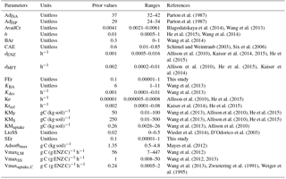
All parameters optimized for ORCHIMIC and their prior values and ranges are listed in Table 2. Considering that the incubation experiment was conducted at constant temperature and pH, parameters related to these variables could not be optimized and were excluded from the optimization. Also, cellulose was the only type of FOM, so adjLS was set to one. The observed variables used in the optimization are listed in Table 3. All the parameters with prescribed non-optimized values are listed in Table 4; while all parameters and observed variables used in the optimization for the CENTURY and PRIM models are summarized in Tables S1 and 3, respectively. For the R observation error matrix, the uncertainties of RF, RS and RSCtrl were set at 5 % of their mean observed values. The priming effect is the difference between RS and RSCtrl, so its uncertainty was set at 10 % of the mean priming effect. The uncertainties of B and BCtrl were both set at 5 % of observed value; whilst the uncertainty of BFOMr was set at 10 % of the observed value. The uncertainties of unknown parameters were set at 10 % of their range. The number of parameters and observations used in the optimization are summarized in Table 5.
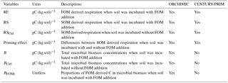
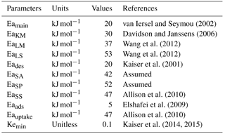
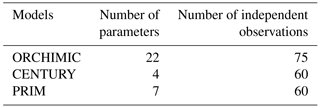
Table 5Number of parameters and observations used in the optimization for each model.
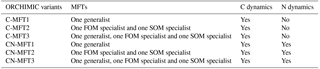
To investigate the effects of including different numbers of MFTs in addition to N dynamics, optimizations were performed with six variants of ORCHIMIC (C-MFT1, C-MFT2, C-MFT3, CN-MFT1, CN-MFT2 and CN-MFT3) summarized in Table 6. C-only means no nitrogen dynamics are considered and the number after MFT indicates the number of MFTs used in each variant of ORCHIMIC (see details in Table 6). The gradient-based iterative algorithm L-BFGS-B (limited-memory Broyden–Fletcher–Goldfarb–Shanno algorithm) (Zhu et al., 1995) was used to minimize the cost function. As this approach may find local minima that differ from the absolute minimum of the complex function J(x), it is very sensitive to the choice of initial parameter values. Guenet et al. (2016) performed 30 optimizations by assigning random initial values within a priori ranges to six parameters to reduce the sensitivity of the solution to the occurrence of local minima. This method proved to be effective for avoiding potential local minima (Santaren et al., 2014). Considering the number of parameters that needed to be optimized in this model, 400 sets of random initial parameter values within their ranges were applied as initial conditions to perform optimizations for each model.
Table 6Descriptions of the six ORCHIMIC variants with or without N dynamics and considering different combinations of MFTs.
The six ORCHIMIC variants (Table 6) were forced with a constant input of 1.6 g C (kg soil)−1 h−1 of litter where the C ∕ N ratio and lignin content were set to 50 and 0.2, respectively (Wang et al., 2013). In this study, only the maximum decomposition rate of cellulose was optimized; therefore maximum decomposition rates for C in LM and LS pools were assumed to be the same. As the temperature during the incubations was kept constant at 295.2 K, we also fixed the temperature at 295.2 K. For the CN-MFT1, CN-MFT2 and CN-MFT3 models, N was removed from the Avail pool at each time step to model the uptake of N by vegetation. The size of the flux was chosen so that the total N flux removed from the system, including N losses during decomposition, was equal to the N input. All models were first run to equilibrium, and then three abrupt changes in the model forcings were applied, i.e., doubling the FOM input, increasing the temperature by 5 K and both together.
6.1 Respiration and priming effect during the incubation experiment
The model simulations shown in Fig. 3 were obtained using the optimized parameters listed in Table 7 for the ORCHIMIC variants and Table S1 in the Supplement for the CENTURY and PRIM models. The observed respiration rate from FOM was high at the beginning of the experiment, shortly after the initial addition of labeled cellulose and gradually increased at a slow rate. Both CENTURY and PRIM underestimated FOM derived respiration at the beginning and overestimated it at the end. Similar results were found for SOM respiration flux, with and without FOM addition (Fig. 3b and c). The modeled respiration from FOM and SOM by all variants of ORCHIMIC were similar and reproduced the observed trend.
Table 7Optimized values and uncertainties of parameters for the six variants of the ORCHIMIC model.
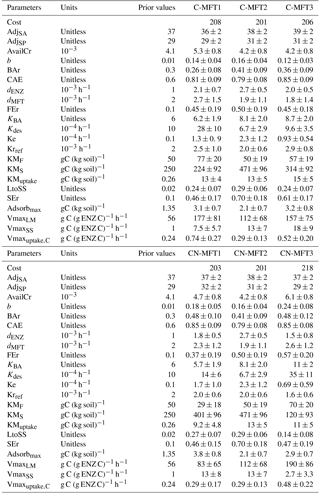
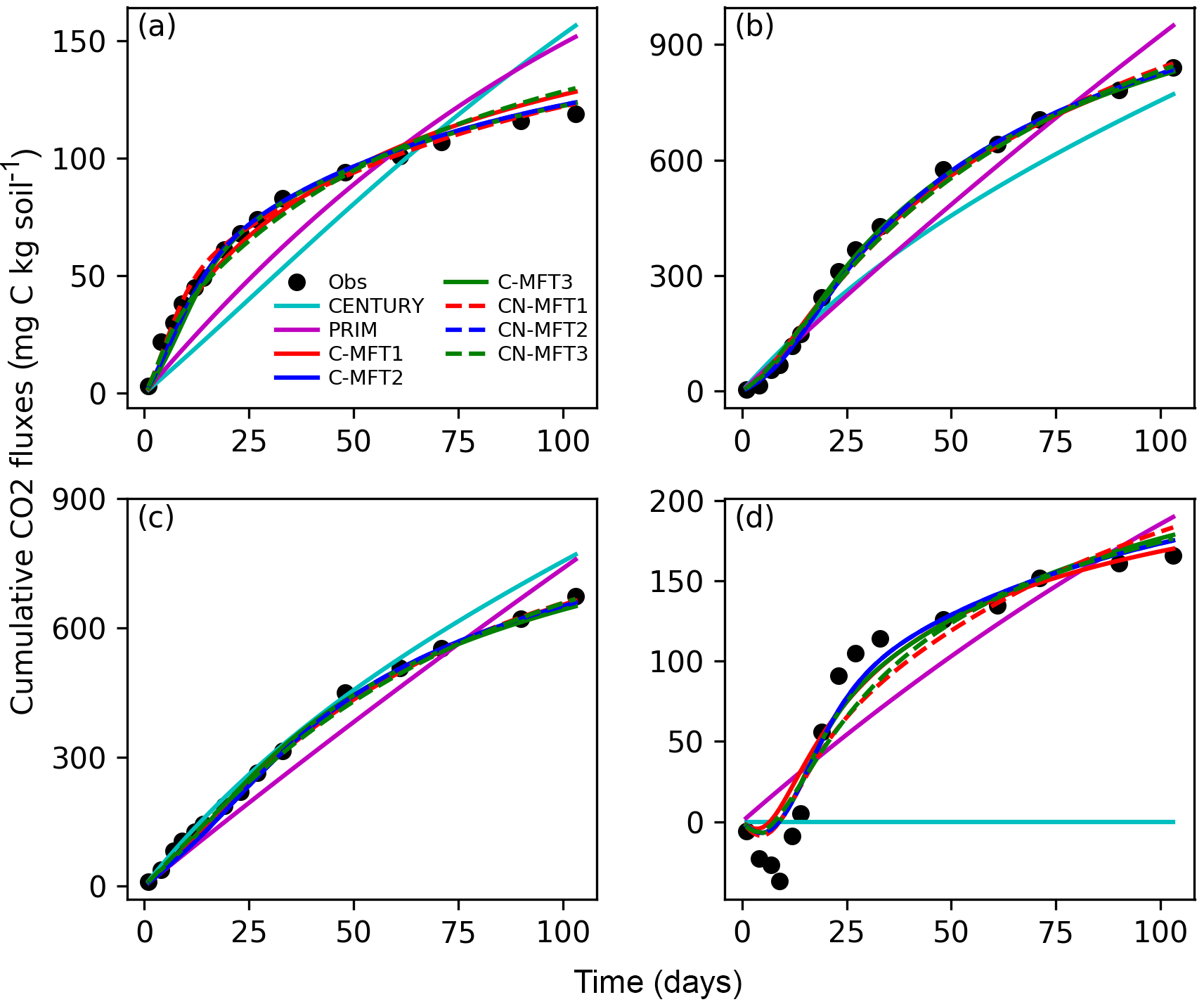
Figure 3Modeled and observed cumulative respiration from (a) FOM, (b) SOM with FOM addition, (c) SOM without FOM addition and (d) priming effect (difference between measured SOM derived respiration with FOM addition minus without FOM addition) (C-MFT2 overlapped with CN-MFT2).
The observed cumulative priming effect, diagnosed as the difference (RS−RSCtrl) between CO2 fluxes derived from SOM with and without FOM addition, was negative for the first 12 days and gradually became positive (Fig. 3d). Then, the cumulative priming effect increased very quickly from day 14 to day 27; after day 27 the priming effect gradually weakened. The modeled priming effect by CENTURY was always zero – by construction of this model. For PRIM, the modeled cumulative priming effect at the end was 190 mg C (kg soil)−1, which is 14 % higher than that observed. However, the shape of the modeled cumulative PE curve also differed from the observations. The modeled priming effect by PRIM was always positive and weakened very slowly with time (Fig. S1 in the Supplement). This meant the PRIM overestimated the cumulative priming effect at both the beginning and the end; although, the additional C loss through the priming effect was well captured at the end of incubation (day 103) (Fig. 3d). The negative cumulative priming effect as simulated by the various ORCHIMIC variants lasted between 6 and 8 days. Similar to the observations, the modeled cumulative priming effect by the ORCHIMIC variants increased very quickly from day 8 onwards, and subsequently slowed down after 13–17 days. At the end of the experiment (day 103), the modeled cumulative priming effect values from the six ORCHIMIC variants were between 170 and 183 mg C (kg soil)−1, only 2.5–11 % higher than that observed.
It can be argued that ORCHIMIC only does a better job at fitting the incubation data because it has more degrees of freedom than the two other models (Table 5). The Akaike information criterion (AIC) takes this into account (Bozdogan, 1987) by considering the optimized model performance and its number of adjustable parameters. The AIC values for each model are shown in Table S2. The AIC values of the six ORCHIMIC variants are much lower than those of CENTURY and PRIM. The difference in AIC values among the six variants are very small for modeling RF, RS, RSCtrl and overall performance, but C-MFT2 and CN-MFT2 have lower AIC values in modeling the priming effect.

Figure 4Modeled and observed microbial biomass and proportion of FOM derived C in the biomass of different MFTs (curve for C-MFT2 overlapped with CN-MFT2). Solid lines show the evolution of microbial biomass or proportion of FOM derived C in MFT-biomass C with FOM addition; dashed lines show the evolution of microbial biomass without FOM addition. Black filled circles and triangles are the observation with and without FOM addition, respectively.
6.2 Microbial biomass evolution during the incubation
Next, we examine how ORCHIMIC simulates the observed microbial biomass evolution throughout the experiment; the two other models do not explicitly include microbial biomass, so could not be evaluated here. The observed total microbial biomass increased at the beginning and reached its maximum (≥ 442 and ≥ 339 mg C (kg soil)−1 for the treatments with and without FOM addition, respectively) between day 14 and 60, after which it decreased both with and without FOM addition (Fig. 4a). The modeled total microbial biomass from the six ORCHIMIC variants all followed a similar trend. With FOM addition, the biomass reached its maximum value of between 425 and 451 mg C (kg soil)−1 on days 28–30 for the different ORCHIMIC variants. Without FOM addition, the biomass reached its maximum value of between 305 and 325 mg C (kg soil)−1 on days 27–34 for the different ORCHIMIC variants.
According to the observations (14C labeling), the proportion of FOM derived C in MFT-biomass C (BFOMr) increased very quickly and peaked (≥ 18 %) before day 14. From day 14 to day 60, BFOMr declined, but subsequently increased between day 60 and day 103 (Fig. 4b). The modeled BFOMr also increased very quickly and reached its maximum value of 13–16 % on days 9–16 for the different ORCHIMIC variants. Unlike the observations, the modeled BFOMr continued to decrease after day 60 and declined to a value of 10–11 % for the different ORCHIMIC variants.
6.3 Proportion of FOM derived C in the AvailC pool during the incubation

Figure 5Modeled and observed proportions of FOM derived C in the AvailC pool. The curve of the C-MFT2 modeled curve overlaps with the CN-MFT2 curve.
Figure 5 shows the modeled and observed proportions of FOM derived C in the AvailC pool (defined as AvailC,FOMr). In the observations, this quantity was not estimated as the proportion of FOM derived C in the AvailC pool, but as the proportion of FOM derived C in dissolved organic carbon (DOC). Although AvailC is not equal to DOC, we assumed that the proportion of FOM derived C in AvailC and in DOC was similar. The observed proportion of FOM derived C in DOC increased quickly at the beginning and reached its maximum (≥ 9.9 %) before day 14, after which it then gradually decreased to 4.3 % on day 103. The modeled AvailC,FOMr reached their peaks of 29–41 % on days 2–4 for the different ORCHIMIC variants. The modeled proportion of FOM derived C in the AvailC pool on day 103 was 7–10 % for the different ORCHIMIC variants.
6.4 Modeled responses to step increases in temperature and fresh organic matter inputs
6.4.1 Change of microbial biomass, enzymes and respiration
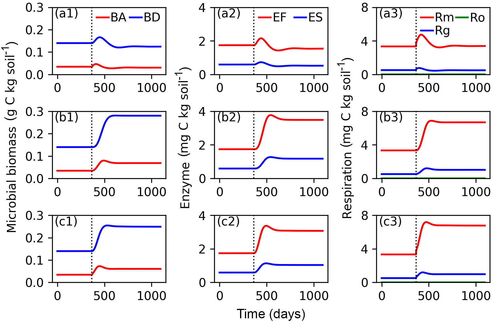
Figure 6Evolutions of active (BA) and dormant (BD) microbial biomass; FOM decomposing enzymes (EF) and SOM decomposing enzymes (ES); and maintenance respiration (Rm), growth respiration (Rg) and overflow respiration (Ro) for CN-MFT3 (standard version of ORCHIMIC) when temperature is stepwise increased by 5 K (a1, a2, a3), when FOM input doubles (b1, b2, b3) and when both forcings are changed (c1, c2, c3). The vertical black dotted line shows the time when the stepwise increase of temperature and/or the doubling FOM input was implemented.
Figure 6 shows that at equilibrium the standard model version CN-MFT3 of ORCHIMIC simulated a total microbial biomass of 0.17 g C (kg soil)−1, with approximately 80 % of the microbes in the dormant and 20 % in the active state. The total enzyme concentration was estimated to be 2.3 mg C (kg soil)−1 and the total respiration was 3.8 mg C (kg soil)−1 d−1, which was equal to the C input rate. When the temperature underwent a stepwise increase of 5 K (panels a in Fig. 6), microbial biomass increased by 19 %, enzyme concentration increased by 12 % and respiration experienced a greater increase of 42 %. However, these effects were ephemeral. After this initial peak, these three pools and fluxes declined and reached new equilibrium values, where microbial biomass was 11 % and enzyme concentrations 12 % below their original values; while the respiration rate returned to its original level, equal to FOM input.
When FOM input was doubled, microbial biomass, enzyme concentration and respiration all increased and equilibrated at a higher level. Both active and dormant microbial biomass increased by 100 %, although active biomass increased faster at the beginning. Hence, the proportion of active biomass increased for about 88 days and reached a peak at 28 % (Fig. S2). Enzyme concentrations almost doubled in response to doubling FOM inputs. Respiration fluxes exactly doubled.
When both doubled FOM input and increased temperature were implemented, the temporal dynamics of microbial biomass, enzyme concentrations and respiration were very similar to those when only the FOM input doubled. At the new equilibrium, only the respiration was doubled and the total microbial biomass and enzyme concentrations increased less (by 77 and 75 %, respectively).
Although the simulated sizes of the different pools were slightly different for the other five variants of ORCHIMIC (Figs. S3–S7), they followed similar trends to those of the standard model version.
6.4.2 Change of soil carbon stock
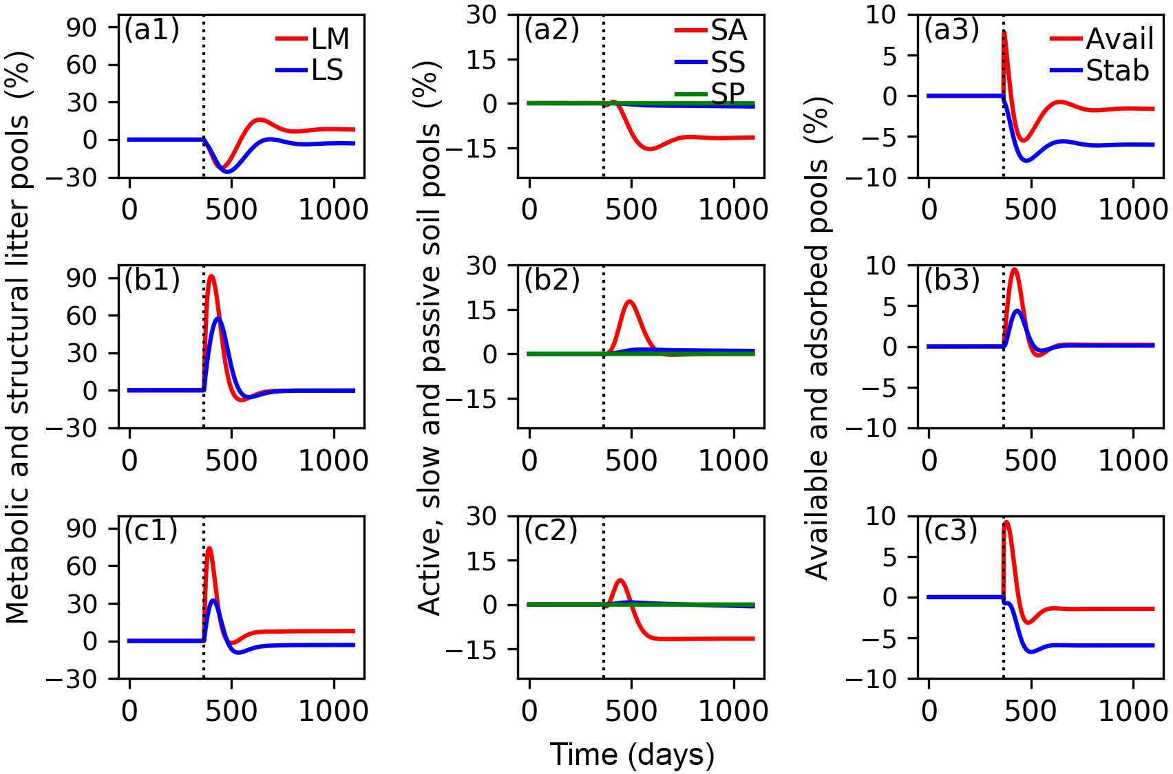
Figure 7Relative changes of C in metabolic (LM) and structural (LS) litter pools (a1, b1, c1); in active (SA), slow (SS) and passive (SP) soil pools (a2, b2, c2); and in available (Avail) and absorbed (Absorb) pools (a3, b3, c3) for the CN-MFT3 model when temperature underwent a stepwise increase of 5 K (a1, a2, a3); when FOM input doubles (b1, b2, b3); and when both a stepwise increase of 5 K and FOM input doubling was implemented (c1, c2, c3). The vertical black dotted line shows the time when the change of temperature and/or FOM input was implemented.
The total SOC content, including microbial biomass and enzymes was 9.7 g C (kg soil)−1 under equilibrium for CN-MFT3. When temperature underwent a stepwise increase of 5 K, there was a fast decrease of C in the litter and SA pools (Fig. 7, results from the other model variants are given in Figs. S8–S12). The loss of C from the LM and LS pools reached 23 % and 26 % of their pre-warming values, respectively. However, the decomposition rates subsequently declined and at equilibrium only 2 % of C was lost from the LS pool; moreover there was even a 9 % increase of C in the LM pool. The C stocks in the SS and SP pools decreased by 4 and 1 %, respectively. C stocks in the SA, Avail and Adsorb pools decreased by 12, 2 and 6 % at the new equilibrium, respectively.
With doubled FOM input, C stocks in all pools increased for a short time but, at the new equilibrium, almost did not change (relative changes were lower than 0.1 % for all pools after 100 years).
When both FOM input was doubled and temperature increased by 5 K, responses were almost the same as in the simulations in which only temperature was increased.
6.4.3 Changes of carbon use efficiency
At equilibrium, the carbon use efficiency (CUE), defined as the ratio of carbon allocated to microbial growth to the sum of that allocated to growth and respiration, was between 0.40 and 0.44 for the different ORCHIMIC variants. When T was increased by 5 K, CUE first fluctuated but finally stabilized at slightly lower values (between 0.39 and 0.42) in all ORCHIMIC variants (Fig. 8a).
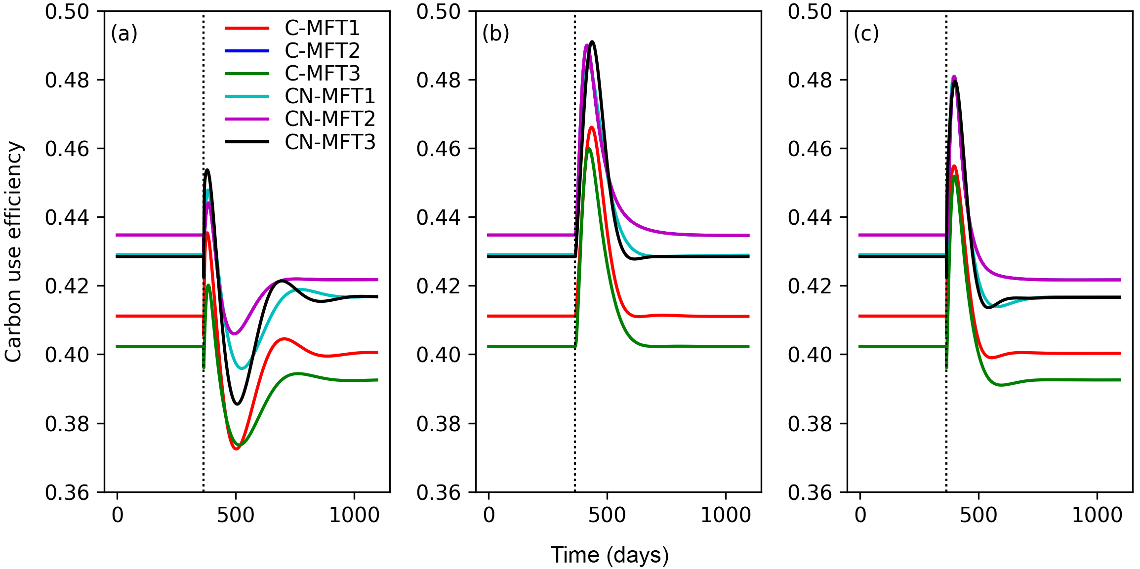
Figure 8Temporal evolution of carbon use efficiencies (defined as ratio of carbon allocated to microbial growth to the sum of those allocated to growth and respiration) when temperature undergoes a stepwise increase of 5 K (a), when FOM input doubles (b) and when both forcings are changed (c), for the six variants of the ORCHIMIC model. The curve for C-MFT2 overlapped with that of CN-MFT2. The vertical black dotted line shows the time when the change of temperature and/or input was applied.
When FOM input was doubled, CUE transiently increased for 52–73 days to a maximum value between 0.46 and 0.49 for the different ORCHIMIC variants. At the new equilibrium, however, CUE was similar to its original level in all ORCHIMIC variants (Fig. 8b).
When T underwent a stepwise increase of 5 K and FOM input doubled, CUE responses were in between those of warming and those of increased FOM additions. At equilibrium, however, the CUE response was similar to that of the T-only treatment for all ORCHIMIC variants (Fig. 8c).
7.1 Optimized parameter vs. literature values
The optimized values for most parameters were generally consistent with those used by previous models and those observed. For example, the ratios of the decomposition rates for the active to slow SOC pool and for the slow to the passive pool were close to those used in the original CENTURY model (Parton et al., 1987). The optimized turnover rate of enzymes (0.035–0.065 d−1 for the six ORCHIMIC variants) was within the range of observed turnover rates for enzymes (0.002–0.10 d−1) (Schimel et al., 2017) and also of a similar magnitude to those used in the models of Allison et al. (2010) (0.024 d−1), He et al. (2015) (0.012–0.048 d−1), Schimel and Weintraub (2003) (0.05 d−1) and Lawrence et al. (2009) (0.05 d−1). The optimized maximum C uptake rate of microbes (0.29–0.74 h−1) was higher, but nonetheless of the same order of magnitude than the value of 0.24 h−1 used by Allison et al. (2010); however, they were much higher than the value of 0.0005 h−1 used by Wang et al. (2013). The optimized value of the death rate of active microbes (0.0015–0.0027 h−1) was consistent with observations. For example, the measured death rate for total microbial biomass at 298.15 K was 0.016 d−1 (Joergensen et al., 1990). Hence, considering an active biomass proportion of 4–49 %, the death rate for active biomass would be 0.0014–0.017 h−1. The optimized death rate for active microbial biomass was also consistent with those used for active biomass by He et al. (2015) (0.0002–0.002 h−1), and comparable to those used by Allison et al. (2010) and Lawrence et al. (2009) (0.0002 and 0.0021 h−1 for total microbial biomass, respectively) if considering an active biomass proportion of 4–49 % (Van de Werf and Verstraete, 1987). Other optimized parameter values that were directly comparable to observations were also consistent with empirical data. For example, the proportion (0.0042–0.0053) of initial AvailC in total SOC was close to the value of 0.0041 for the proportion of DOC in total SOC reported by Blagodatskaya et al. (2014) for the incubated soil. The initial active microbial biomass proportion was 26–48 % of the total biomass, lying in the observed range of 4–49 % reported by Van de Werf and Verstraete (1987).
Some other optimized parameters differed substantially from the values used in previous models, yet were consistent with those observed. For example, the ratio of maintenance respiration in dormant relative to active microbes (0.12–0.24) was within the range reported by Wang et al. (2014) (0.025–0.351) which was estimated based on data from two incubation experiments, but much higher than that used in the model of He et al. (2015) (0.0005–0.005). The optimized CAE of 0.8 was also higher than the value of 0.5 used by Schimel and Weintraub (2003), yet close to the value (0.8) for CAE of reserve metabolites used in the model of Tang and Riley (2015). A wide range of CUE (0.01–0.85) was reported by Six et al. (2006) in a review of studies measuring CUE. High CUE (0.67–0.75) was also reported by Hagerty et al. (2014). These high values indicate that CAE could be as high as 0.8 because CAE should be larger than CAE, which is due to the fact that CUE takes maintenance respiration into account. The maximum decomposition rates of substrates were higher than those used in previous models (Allison et al., 2010; Wang et al., 2013; Kaiser et al., 2014, 2015). For example, in Wang et al. (2013), the optimized maximum decomposition rates for particulate organic matter and mineral-associated organic matter were 2.5 and 1.0 mg C (mg enzyme C)−1 h−1, respectively, while 0.24 mg C (mg enzyme C)−1 h−1 was used as maximum decomposition rate for soil organic matter in the model of Allison et al. (2010). However, the maximum decomposition rate for cellulose optimized from our study was 83 to 190 mg C (mg enzyme C)−1 h−1. One likely explanation for such a large difference is that the data used by Wang et al. (2013) and Allison et al. (2010) were to be applied to the decomposition of SOM or litter; however, in this study, the main substrate was cellulose which was milled before being added to soil and was also well mixed within the soil during the incubation experiment. Moreover, cellulose has a very homogeneous structure and is, therefore, easy to decompose. In any case, the maximum decomposition rate is within the range reported by laboratory measurements for cellulose. For example, according to data collected by Wang et al. (2012), the maximum decomposition rate of cellulose could be as high as 7900 mg C (mg enzyme C)−1 h−1 with an average value of 80 mg C (mg enzyme C)−1 h−1.
7.2 Performance of ORCHIMIC model
The ORCHIMIC model generally performed better than CENTURY and PRIM. Despite the larger number of parameters, the AIC values for the six variants of ORCHIMIC were lower than those of the more parsimonious CENTURY and PRIM models. The decomposition rates in CENTURY follow first-order kinetics (Parton et al., 1987) and do not interact; therefore, with and without FOM addition the SOM derived respiration is always the same and priming can not be captured. The PRIM model was developed with the aim of modeling the priming effect (Guenet et al., 2016). The decomposition rate of FOM still follows first-order kinetics, so FOM derived respiration has a similar trend to that in the CENTURY model. However, the decomposition rate of more recalcitrant SOC is accelerated when the FOM pool is higher, as is the case in incubations with FOM (cellulose) addition. Hence, SOM derived respiration will increase and lead to a positive priming effect of rather constant magnitude for the simulations where cellulose is added. In contrast, the ORCHIMIC model variations with different numbers of MFTs and with or without N dynamics all better captured the temporal dynamics of both respiration and priming effects as measured by Blagodatskaya et al. (2014).
In ORCHIMIC, the substrate decomposition rate is nonlinear because ECA kinetics are applied to simulating substrate decomposition (Eqs. 20–24). The decomposition rate becomes lower as the substrate gradually depletes (Fig. 3a) because the incubation experiments do not have a continuous input of C like in the real world. This model result is consistent with observations of decelerating respiration at the end of the incubation (Fig. 3a). In ORCHIMIC, the depletion of substrates lowers the saturation ratio of the substrate pool and subsequently inhibits the production of enzymes and reduces the decomposition rate of the substrates. The resulting lower saturation ratio of the Avail pool then triggers dormancy and reduces the growth rate of active microbial biomass, which in turn reduces enzyme production and thereby generates a positive feedback to reduced decomposition. As a result, SOM mineralization rates and respiration rates slow down at the end of the incubation experiment.
The main mechanism underlying the positive priming effect in ORCHIMIC is that the FOM input stimulates the growth of active microbes and the transformation of dormant states to active states. This in turn leads to increased enzyme production and thereby the faster mineralization of SOM. However, at the beginning, the fast mineralization of FOM decreases the fraction of SOM derived C in the Avail pool. The total respiration does not change much, but less respired C is SOM derived, thus, creating a negative priming effect. Furthermore, because dynamic enzyme production is applied, the increase of the saturation ratio of the Avail pool due to FOM addition suppresses enzyme production per unit of active biomass; this suppression then slows down the increase of, or even decreases, the size of the SOM decomposition enzyme pool, which partly suppresses SOM derived respiration.
ORCHIMIC reproduced the observed microbial biomass, a variable which is not modeled by CENTURY and PRIM. Also, the transfer of FOM derived C to the Avail pool and the assimilation of FOM derived C into microbial biomass were well captured (Figs. 4b and 5). However, the observed increased contribution of FOM derived C in microbial biomass during the incubation was not reproduced by ORCHIMIC. This suggests that some important processes related to microbial biomass are misrepresented or still lacking. As there was no such increase for DOC, the increase of the proportion of FOM derived C in microbial biomass was probably not due to the increased uptake of FOM derived C. Therefore, this is probably related to microbial turnover, which is homogeneous for old (more is SOM derived) and new (more is FOM derived) microbial biomass C in ORCHIMIC.
With the same FOM input but under a lower temperature 285.15 K, Wang et al. (2013) simulated a SOC stock of about 17 g C (kg soil)−1, which was 2–3 times the value simulated here. This may be attributed to the much smaller decomposition rates applied in their model. In our study, the equilibrium C concentration in the Avail pool was 0.11–0.32 g C (kg soil)−1, comparable with 0.16 g C (kg soil)−1 in their model for dissolved organic carbon (DOC), and within one standard deviation interval of the range (0.04–0.52 g C (kg soil)−1) reported in the literature (Wang et al., 2013). In ORCHIMIC, the total enzyme concentration at equilibrium was 1.78–5.75 mg C (kg soil)−1, which was close to the reported upper range (0.01–5 mg C (kg soil)−1) for α-glucosidase and β-glucosidase concentrations in soil by Tabatabai (2003). However, considering that many kinds of enzymes exist in soil, Wang et al. (2003) used a value of 1 mg C (kg soil)−1 when estimating parameter values for their model. Hence, the enzyme concentrations simulated by ORCHIMIC are probably realistic. ORCHIMIC generated a reasonable proportion of microbial biomass in the total soil C stock (1.8–4.4 %), which is around the global average of in situ measurements compiled by Xu et al. (2013). The active biomass proportion was also close to that reported by Van de Werf and Verstraete (1987) (19 ± 9 %), by Lennon and Jones (2011) (18 ± 15 %) and by Stenström et al. (2001) (5–20 %).
All soil C pools except LM, decreased in response to warming, which was consistent with the simulations from conventional SOM decomposition models. Unlike other pools, there was an increase in the LM pool, because the increase of the decomposition rate per unit of enzymes was relatively small. This was due to the lower temperature sensitivity of the decomposition of LM (prescribed smallest Ea for LM in ORCHIMIC) and it was compensated for by the decreased enzyme concentration. The soil C pools remained practically unchanged, although microbial biomass doubled, with double FOM inputs, as increasing FOM accelerated the decomposition of SOM by stimulating the growth of microbes and the production of enzymes. These responses were different from the proportional increase in soil C pools as modeled by the conventional linear SOC decomposition model, but consistent with those observed from microbial models with a linear microbial death rate (Wang et al., 2013, 2016). It should be noted that with density-dependent microbial mortality, the growth of microbes owing to an increase of FOM input might be limited and lead to accumulation of soil C (Georgiou et al., 2017). With double FOM input and warming, the modeled SOC stock from ORCHIMIC decreased instead of increasing as modeled by conventional linear SOC decomposition models. This was due to the fact that the priming effect induced by FOM addition compensated for the increased C input to the soil, and also because the increased SOC decomposition rate due to warming decreased the SOC stock.
7.3 Comparison of six ORCHIMIC variants
Regarding the simulation of respiration, the priming effect and microbial biomass, the cost function value at the minimum was the smallest for the two ORCHIMIC model variants with two MFTs and largest for the more comprehensive standard version CN-MFT3 (Table 7). Thus, any improvements associated with having more MFTs or including N dynamics in the model are not apparent when using the Blagodatskaya et al. (2014) measurements. In ORCHIMIC, the main differences among the MFTs are their different C ∕ N ratios and the ability to produce two kinds of enzymes. Although ORCHIMIC can simulate different enzyme concentrations with different MFTs, their effects were partly offset by the different maximum decomposition rates for the different enzymes; therefore models with more MFTs are not always better than models with fewer MFTs. Furthermore, there is the assumption that the initial biomass and active biomass proportion of each MFT limited the performance of the model with more MFTs.
According to our simulations for the different temperature and FOM-addition scenarios, the amount of N required for microbial growth was only 10 % of the initial DON in the incubated soil. Therefore, sufficient N was available to feed microbial demand, explaining why the model set ups without the N cycle behaved similarly to those with the representation of the N cycle. Future applications of this model, using N-limited soils are needed to assess the degree to which N cycling needs to be represented in the SOC models. Because the long-term limitation of N on microbial growth was absent from our study, we can not yet evaluate the potential improvements by including N dynamics in the model.
When N is considered, N-limited conditions favor the growth of MFTs with larger C ∕ N ratios, while C-limited conditions favor the growth of MFTs with smaller C ∕ N ratios. Also, different major sources (FOM or SOM) of C and N favor different MFTs depending on their enzyme production cost. Thus, with more than one MFT, the C ∕ N ratio of the microbial pool can be variable (Figs. S13–S15).
7.4 Dynamic enzyme production
Unlike some microbial models where enzyme production depends solely on microbial biomass or microbial uptake, the saturation level of substrate is an important factor affecting enzyme production in ORCHIMIC. Microbes increase enzyme production if there is more substrate available to grow faster, and they decrease enzyme production when the substrate is depleting to avoid unnecessary allocation of C and N to the enzyme production function. In ORCHIMIC, the saturation level of directly available C also affects enzyme production. Enzyme production per unit of microbial biomass decreases with increasing available C (see Eq. 53), e.g., via catabolic repression of enzyme synthesis by the product of the reaction. This also corresponds to the fact that the fraction of cheaters – microbes that do not produce enzymes – increases with increasing available C. Cheaters were added as an explicit microbial functional group in an individual-based micro-scale microbial community model with the explicit positioning of microbes to access substrate (Kaiser el al., 2015). Such an approach is only applicable in a micro-scale model, as the coexistence of cheaters and enzyme-producing microbes is only sustainable in heterogeneous environments. In non-spatially explicit zero-dimensional models, like ORCHIMIC, which assume a homogeneous environment, cheaters will always have a competitive advantage over other microbes in taking up C and N while not having to invest in enzyme production. This will eventually drive enzyme-producing MFTs to extinction at steady state (Allison, 2005); the model will not produce enzymes anymore and all microbes will die in the end. With the dynamic enzyme production mechanism described in Eqs. (51)–(55), cheaters can be included in ORCHIMIC in a possible coexistence with non-cheater microbes in the model, although cheaters are not parameterized in an explicit way as a separate MFT group.
7.5 Changes in carbon use efficiency with warming and increased FOM input
The ORCHIMIC model suggested that, upon a 5 K stepwise increase of temperature, CUE initially decreased by 0.05–0.08 due to the immediate increase of maintenance respiration in response to the higher temperature. However, at equilibrium, the change in temperature induced a decrease of the CUE by 0.0018–0.0026 K−1, relative to the equilibrium at lower temperature. The activation energy is a key factor regulating the response of the maintenance respiration cost to warming. In this study, the activation energy for maintenance respiration was set to 20 kJ mol−1 (van Iersel and Seymour, 2002), while 60 kJ mol−1 was used by Tang and Riley (2015). A larger activation energy implies lower respiration rates, but also a larger temperature sensitivity of respiration; thus it also infers a larger relative increase of the maintenance cost and a larger decrease of the CUE when temperature increases (Davidson and Janssens, 2006; Davidson et al., 2012). Although not always consistent among experimental studies (Dijkstra et al., 2011), a decrease of the CUE with warming has often been observed. For example, Van Ginkel et al. (2000) showed that the sensitivity of the CUE in response to warming could be as large as −0.049 K−1 and Steinweg et al. (2008) found a CUE sensitivity to warming value of −0.009 K−1. After considering the effect of temperature on the turnover of microbial biomass, Hagerty et al. (2014) estimated a decrease of the CUE by 0.005 and 0.003 K−1 for mineral and organic soil, respectively. There are indications that the temperature response of the CUE varies with substrate and temperature. For example, in the study of Devêvre and Horwáth (2000), when temperature increased from 278.15 to 288.15 K, the CUE decreased by 0.021 and 0.015 K−1 when the soil was incubated with low C ∕ N and high C ∕ N of FOM, respectively. This study also showed that, when temperature increased further from 288.15 to 298.15 K, the decrease in the CUE was only 0.006 K−1. Thus, it seems that the CUE tends to decrease more slowly when the applied temperature warming or the C ∕ N ratio of FOM is higher. If this is true, then the relatively low decrease in CUE of 0.0018–0.0026 K−1 that we observed was to be expected.
Besides temperature and the substrate's C ∕ N ratio, the decomposition rate of the substrate is also an important factor affecting the CUE. Normally, CUE is higher for substrates with higher decomposition rates, because the maintenance costs remain relatively stable (del Giorgio and Cole, 1998; van Bodegom, 2007). As such, the short-lived increase of the CUE that we observed in Fig. 8 after the temperature was increased by 5 K may be related to the increase of the maximum decomposition rate for each substrate with temperature. Furthermore, with doubled FOM input, a longer increase of the CUE was observed compared to that found with the 5 K stepwise increase in temperature. However, at the new equilibrium, with doubled FOM inputs, the respiration doubled because microbial biomass also doubled, and therefore the CUE remained almost unchanged.
7.6 Implications
Increased greenhouse gases in the atmosphere warm air temperature, and subsequently soil temperature, which increases primary productivity in regions where water or nutrients are not scarce. Thus, increases in both the input and the decomposition rates of SOM are expected (Jones et al., 2005). The response of SOC to these two drivers (input and decomposition rates) is determined by complex processes; however current SOC decomposition models used in Earth system models (ESM) always simulate that increased input leads to increased storage of SOC, and that soil warming leads to decreased storage from increased decomposition rates. Despite different pathways of CO2 emission scenarios, SOC stocks tends to increase in the near future in most ESMs (Burke et al., 2017; Todd-Brown et al., 2014). In ORCHIMIC, as shown in Fig. 7 for the 5 K and doubled FOM input simulations, the canonical model response is that SOC stocks are projected to decrease instead of increasing, implying a totally different response of SOC stock to future climate change than that projected by conventional linear SOC decomposition models.
The ORCHIMIC variant CN-MFT3 does not obviously perform better than the variants with less MFTs or even those without N dynamics in reproducing the results from incubation experiments. However, CN-MFT3, as the standard version of ORCHIMIC, is preferable due to the fact that it is able to model the dynamic C ∕ N ratio of the microbial community and is also more accurate in modeling the dynamics of soil SOM pools, including microbial biomass pools under N-limited conditions.
Despite the complexity of ORCHIMIC compared to the current SOC models embedded in ESMs for large-scale applications, the main soil carbon and litter pools in the model are defined similarly to those of ESMs. Most of the input variables (like litter fall and plant N uptake), and environmental conditions (soil moisture and temperature) can also be directly calculated by the ESM. Furthermore, the time step of ORCHIMIC is similar to that of most ESMs (i.e., daily), which makes it possible to embed ORCHIMIC into most current ESMs. As ORCHIMIC includes key processes related to microbial communities that can be measured in experiments, it provides the basis for a refined representation of global change effects on soil C by integrating intertwined processes such as soil nutrient availability and organic matter inputs.
We developed a soil C and N model with a dynamic enzyme production mechanism and a microbial dormancy strategy considered for four microbial function groups: generalists, FOM specialists and SOM specialists are explicitly represented and cheaters are inexplicitly included. This newly developed ORCHIMIC model not only reproduces respiration, but also the priming effect. Moreover, it can reproduce several measurable variables, such as microbial biomass, which includes not only the total microbial biomass but also the fractions of active microbial biomass and the SOM and FOM derived C in the total microbial biomass. In addition, with realistic inputs, ORCHIMIC generated realistic SOC stocks, microbial biomass, proportion of microbial biomass in the SOC stock, proportion of active microbial biomass in total microbial biomass, as well as enzyme concentrations. Finally, ORCHIMIC can be easily integrated into ESMs for more realistic predictions of changes in SOM under future scenarios.
The ORCHIMIC v1.0 is programmed in the Python programming language. In order to run the model the basic Python packages numpy, os and sys must be preinstalled. The source code, optimized parameter values and script used to reproduce the results (shown in Sect. 6.4) are available online (https://github.com/huangysmile/ORCHIMIC/releases/tag/v1.0; DOI: https://doi.org/10.5281/zenodo.1164740, Huangysmile, 2018).
In the above equations Fθ, FT,j, FpH, Fclay and Flignin are the respective functions of soil moisture, temperature, pH, clay content and lignin content with the same definitions in ORCHIMIC; AdjLS, AdjSA and AdjSP are also defined the same way as in ORCHIMIC; KLM and KSS are the decomposition rates of C in LM and SS pools, respectively; DSA,CENT, DSS,CENT and DSP,CENT are decomposition fluxes of C for the SA, SS and SP pools in CENTURY, respectively; and DSA,PRIM, DSS,PRIM and DSP,PRIM are the respective decomposition fluxes of C for SA, SS and SP pools in PRIM.
The supplement related to this article is available online at: https://doi.org/10.5194/gmd-11-2111-2018-supplement.
The authors declare that they have no conflict of interest.
Funding for the study was supported by the European Research Council
through the Synergy grant ERC-2013-SyG610028
“IMBALANCE-P”.
Edited by: Carlos
Sierra
Reviewed by: two anonymous referees
Allison, S. D.: Cheaters, diffusion and nutrients constrain decomposition by microbial enzymes in spatially structured environments, Ecol. Lett., 8, 626–635, 2005.
Allison, S. D. and Vitousek, P. M.: Responses of extracellular enzymes to simple and complex nutrient inputs, Soil Biol. Biochem., 37, 937–944, 2005.
Allison, S. D., Wallenstein, M. D., and Bradford, M. A.: Soil-carbon response to warming dependent on microbial physiology, Nat. Geosci., 3, 336–340, 2010.
Anav, A., Friedlingstein, P., Kidston, M., Bopp, L., Ciais, P., Cox, P., Jones, C., Jung, M., Myneni, R., and Zhu, Z.: Evaluating the Land and Ocean Components of the Global Carbon Cycle in the CMIP5 Earth System Models, J. Climate, 26, 6801–6843, 2013.
Arora, V. K., Boer, G. J., Friedlingstein, P., Eby, M., Jones, C. D., Christian, J. R., Bonan, G., Bopp, L., Brovkin, V., Cadule, P., Hajima, T., Ilyina, T., Lindsay, K., Tjiputra, J. F., and Wu, T.: Carbon–Concentration and Carbon–Climate Feedbacks in CMIP5 Earth System Models, J. Climate, 26, 5289–5314, 2013.
Batjes, N. H.: Total carbon and nitrogen in the soils of the world, Eur. J. Soil Sci., 65, 10–21, 2014.
Blagodatskaya, A. and Kuzyakov, Y.: Mechanisms of real and apparent priming effects and their dependence on soil microbial biomass and community structure: critical review, Biol. Fert. Soils, 45, 115–131, 2008.
Blagodatskaya, E. and Kuzyakov, Y.: Active microorganisms in soil: Critical review of estimation criteria and approaches, Soil Biol. Biochem., 67, 192–211, 2013.
Blagodatskaya, E., Khomyakov, N., Myachina, O., Bogomolova, I., Blagodatsky, S., and Kuzyakov, Y.: Microbial interactions affect sources of priming induced by cellulose, Soil Biol. Biochem., 74, 39–49, 2014.
Bozdogan, H.: Model selection and Akaike's Information Criterion (AIC): The general theory and its analytical extensions, Psychometrika, 52, 345–370, 1987.
Burke, E. J., Ekici, A., Huang, Y., Chadburn, S. E., Huntingford, C., Ciais, P., Friedlingstein, P., Peng, S., and Krinner, G.: Quantifying uncertainties of permafrost carbon–climate feedbacks, Biogeosciences, 14, 3051–3066, https://doi.org/10.5194/bg-14-3051-2017, 2017.
Creamer, C. A., de Menezes, A. B., Krull, E. S., Sanderman, J., Newton-Walters, R., and Farrell, M.: Microbial community structure mediates response of soil C decomposition to litter addition and warming, Soil Biol. Biochem., 80, 175–188, 2015.
Davidson, E. A. and Janssens, I. A.: Temperature sensitivity of soil carbon decomposition and feedbacks to climate change, Nature, 440, 165–173, 2006.
Davidson, E. A., Samanta, S., Caramori, S. S., and Savage, K.: The Dual Arrhenius and Michaelis–Menten kinetics model for decomposition of soil organic matter at hourly to seasonal time scales, Glob. Change Biol., 18, 371–384, 2012.
del Giorgio, P. A. and Cole, J. J.: Bacterial Growth Efficiency in Natural Aquatic Systems, Annu. Rev. Ecol. Syst., 29, 503–541, 1998.
Devêvre, O. C. and Horwáth, W. R.: Decomposition of rice straw and microbial carbon use efficiency under different soil temperatures and moistures, Soil Biol. Biochem., 32, 1773–1785, 2000.
Dijkstra, P., Thomas, S. C., Heinrich, P. L., Koch, G. W., Schwartz, E., and Hungate, B. A.: Effect of temperature on metabolic activity of intact microbial communities: Evidence for altered metabolic pathway activity but not for increased maintenance respiration and reduced carbon use efficiency, Soil Biol. Biochem., 43, 2023–2031, 2011.
D'Odorico, P., Laio, F., Porporato, A., and Rodriguez-Iturbe, I.: Hydrologic controls on soil carbon and nitrogen cycles. II. A case study, Adv. Water Resour., 26, 59–70, 2003.
Elshafei, G. S., Nasr, I. N., Hassan, A. S. M., and Mohammad, S.: Kinetics and thermodynamics of adsorption of cadusafos on soils. J. Hazard. Mater., 172, 1608–1616, 2009.
Fontaine, S., Mariotti, A., and Abbadie, L.: The priming effect of organic matter: a question of microbial competition?, Soil Biol. Biochem., 35, 837–843, 2003.
Friedlingstein, P.: Carbon cycle feedbacks and future climate change, Philos. T. R. Soc. A., 373, 20140421, https://doi.org/10.1098/rsta.2014.0421, 2015.
Georgiou, K., Abramoff, R. Z., Harte, J., Riley, W. J., and Torn, M. S.: Microbial community-level regulation explains soil carbon responses to long-term litter manipulations, Nat. Commun., 8, 1223, https://doi.org/10.1038/s41467-017-01116-z, 2017.
Guenet, B., Juarez, S., Bardoux, G., Abbadie, L., and Chenu, C.: Evidence that stable C is as vulnerable to priming effect as is more labile C in soil, Soil Biol. Biochem., 52, 43–48, 2012.
Guenet, B., Moyano, F. E., Peylin, P., Ciais, P., and Janssens, I. A.: Towards a representation of priming on soil carbon decomposition in the global land biosphere model ORCHIDEE (version 1.9.5.2), Geosci. Model Dev., 9, 841–855, https://doi.org/10.5194/gmd-9-841-2016, 2016.
Hagerty, S. B., van Groenigen, K. J., Allison, S. D., Hungate, B. A., Schwartz, E., Koch, G. W., Kolka, R. K., and Dijkstra, P.: Accelerated microbial turnover but constant growth efficiency with warming in soil, Nat. Clim. Change, 4, 903–906, 2014.
Hamer, U. and Marschner, B.: Priming effects in different soil types induced by fructose, alanine, oxalic acid and catechol additions, Soil Biol. Biochem., 37, 445–454, 2005.
Hararuk, O., Xia, J., and Luo, Y.: Evaluation and improvement of a global land model against soil carbon data using a Bayesian Markov chain Monte Carlo method, J. Geophy. Res.-Biogeo., 119, 403–417, 2014.
He, Y., Yang, J., Zhuang, Q., Harden, J. W., McGuire, A. D., Liu, Y., Wang, G., and Gu, L.: Incorporating microbial dormancy dynamics into soil decomposition models to improve quantification of soil carbon dynamics of northern temperate forests, J. Geophys. Res.-Biogeo., 120, 2015JG003130, https://doi.org/10.1002/2015JG003130, 2015.
Huangysmile: huangysmile/ORCHIMIC: ORCHIMICv1.0 (Version v1.0), Zenodo, https://doi.org/10.5281/zenodo.1164740), 2018.
Janssens, I. A., Dieleman, W., Luyssaert, S., Subke, J.-A., Reichstein, M., Ceulemans, R., Ciais, P., Dolman, A. J., Grace, J., Matteucci, G., Papale, D., Piao, S. L., Schulze, E.-D., Tang, J., and Law, B. E.: Reduction of forest soil respiration in response to nitrogen deposition, Nat. Geosci., 3, 315–322, 2010.
Jenkinson, D. S., Adams, D. E., and Wild, A.: Model estimates of CO2 emissions from soil in response to global warming, Nature, 351, 304–306, 1991.
Jobbágy, E. G. and Jackson, R. B.: The Vertical Distribution of Soil Organic Carbon and Its Relation to Climate and Vegetation, Ecol. Appl., 10, 423–436, 2000.
Joergensen, R. G., Brookes, P. C., and Jenkinson, D. S.: Survival of the soil microbial biomass at elevated temperatures, Soil Biol. Biochem., 22, 1129–1136, 1990.
Jones, C., McConnell, C., Coleman, K., Cox, P., Falloon, P., Jenkinson, D., and Powlson, D.: Global climate change and soil carbon stocks; predictions from two contrasting models for the turnover of organic carbon in soil, Glob. Change Biol., 11, 154–166, 2005.
Kaiser, K., Kaupenjohann, M., and Zech, W.: Sorption of dissolved organic carbon in soils: effects of soil sample storage, soil-to-solution ratio, and temperature, Geoderma, 99, 317–328, 2001.
Kaiser, C., Franklin, O., Dieckmann, U., and Richter, A.: Microbial community dynamics alleviate stoichiometric constraints during litter decay, Ecol. Lett., 17, 680–690, 2014.
Kaiser, C., Franklin, O., Richter, A., and Dieckmann, U.: Social dynamics within decomposer communities lead to nitrogen retention and organic matter build-up in soils, Nat. Commun., 6, 8960, https://doi.org/10.1038/ncomms9960, 2015.
Koroljova-Skorobogat'ko, O. V., Stepanova, E. V., Gavrilova, V. P., Morozova, O. V., Lubimova, N. V., Dzchafarova, A. N., Jaropolov, A. I., and Makower, A.: Purification and characterization of the constitutive form of laccase from the basidiomycete Coriolus hirsutus and effect of inducers on laccase synthesis, Biotechnol. Appl. Bioc., 28, 47–54, 1998.
Kothawala, D. N., Moore, T. R., and Hendershot, W. H.: Adsorption of dissolved organic carbon to mineral soils: a comparison of four isotherm approaches, Geoderma, 148, 43–50, 2008.
Krinner, G., Viovy, N., de Noblet-Ducoudré, N., Ogée, J., Polcher, J., Friedlingstein, P., Ciais, P., Sitch, S., and Prentice, I. C.: A dynamic global vegetation model for studies of the coupled atmosphere-biosphere system, Global Biogeochem. Cy., 19, GB1015, https://doi.org/10.1029/2003GB002199, 2005.
Kuzyakov, Y. and Bol, R.: Sources and mechanisms of priming effect induced in two grassland soils amended with slurry and sugar, Soil Biol. Biochem., 38, 747–758, 2006.
Kuzyakov, Y., Friedel, J. K., and Stahr, K.: Review of Mechanisms and Quantification of Priming Effects, Soil Biol. Biochem. 32, 1485–1498, 2000.
Lawrence, C. R., Neff, J. C., and Schimel, J. P.: Does adding microbial mechanisms of decomposition improve soil organic matter models? A comparison of four models using data from a pulsed rewetting experiment, Soil Biol. Biochem., 41, 1923–1934, 2009.
Lennon, J. T. and Jones, S. E.: Microbial seed banks: the ecological and evolutionary implications of dormancy, Nat. Rev. Microbiol., 9, 119–130, 2011.
Manzoni, S. and Porporato, A.: Soil carbon and nitrogen mineralization: Theory and models across scales, Soil Biol. Biochem., 41, 1355–1379, 2009.
Mayes, M. A., Heal, K. R., Brandt, C. C., Phillips, J. R., and Jardine, P. M.: Relation between Soil Order and Sorption of Dissolved Organic Carbon in Temperate Subsoils, Soil Sci. Soc. Am. J., 76, 1027–1037, 2012.
MEA: Millennium Ecosystem Assessment – Nutrient Cycling, World Resource Institute, Washington, DC, USA, 2005.
Moorhead, D. L. and Sinsabaugh, R. L.: A Theoretical Model of Litter Decay and Microbial Interaction, Ecol. Monogr., 76, 151–174, 2006.
Mosier, A. R., Parton, W. J., and Hutchinson, G. L.: Modelling Nitrous Oxide Evolution from Cropped and Native Soils, Ecol. Bull., 35, 229–241, 1983.
Mouginot, C., Kawamura, R., Matulich, K. L., Berlemont, R., Allison, S. D., Amend, A. S., and Martiny, A. C.: Elemental stoichiometry of Fungi and Bacteria strains from grassland leaf litter, Soil Biol. Biochem., 76, 278–285, 2014.
Nannipieri, P., Ascher, J., Ceccherini, M. T., Landi, L., Pietramellara, G., and Renella, G.: Microbial diversity and soil functions, Eur. J. Soil Sci., 54, 655–670, 2003.
Parton, W. J., Schimel, D. S., Cole, C. V., and Ojima, D. S.: Analysis of Factors Controlling Soil Organic Matter Levels in Great Plains Grasslands, Soil Sci. Soc. Am. J., 51, 1173, https://doi.org/10.2136/sssaj1987.03615995005100050015x, 1987.
Parton, W. J., Stewart, J. W. B., and Cole, C. V.: Dynamics of C, N, P and S in grassland soils: a model, Biogeochemistry, 5, 109–131, 1988.
Porporato, A., D'Odorico, P., Laio, F., and Rodriguez-Iturbe, I.: Hydrologic controls on soil carbon and nitrogen cycles. I. Modeling scheme, Adv. Water Resour., 26, 45–58, 2003.
Prévost-Bouré, N.C., Soudani, K., Damesin, C., Berveiller, D., Lata, J.-C., and Dufrêne, E.: Increase in aboveground fresh litter quantity over-stimulates soil respiration in a temperate deciduous forest, Appl. Soil Ecol., 46, 26–34, 2010.
Qian, H., Joseph, R., and Zeng, N.: Enhanced terrestrial carbon uptake in the Northern High Latitudes in the 21st century from the Coupled Carbon Cycle Climate Model Intercomparison Project model projections, Glob. Change Biol., 16, 641–656, 2010.
Reth, S., Reichstein, M., and Falge, E.: The effect of soil water content, soil temperature, soil pH-value and the root mass on soil CO2 efflux – A modified model, Plant Soil, 268, 21–33, 2005.
Santaren, D., Peylin, P., Viovy, N., and Ciais, P.: Optimizing a process-based ecosystem model with eddy-covariance flux measurements: A pine forest in southern France, Global Biogeochem. Cy., 21, GB2013, https://doi.org/10.1029/2006GB002834, 2007.
Santaren, D., Peylin, P., Bacour, C., Ciais, P., and Longdoz, B.: Ecosystem model optimization using in situ flux observations: benefit of Monte Carlo versus variational schemes and analyses of the year-to-year model performances, Biogeosciences, 11, 7137–7158, https://doi.org/10.5194/bg-11-7137-2014, 2014.
Schimel, D. S.: Carbon and nitrogen turnover in adjacent grassland and cropland ecosystems, Biogeochemistry, 2, 345–357, 1986.
Schimel, J., Becerra, C. A., and Blankinship, J.: Estimating decay dynamics for enzyme activities in soils from different ecosystems, Soil Biol. Biochem., 114, 5–11, 2017.
Schimel, J. P. and Weintraub, M. N.: The implications of exoenzyme activity on microbial carbon and nitrogen limitation in soil: a theoretical model, Soil Biol. Biochem., 35, 549–563, 2003.
Sinsabaugh, R. L. and Follstad Shah, J. J.: Ecoenzymatic Stoichiometry and Ecological Theory, Annu. Rev. Ecol. Evol. S., 43, 313–343, 2012.
Six, J., Frey, S. D., Thiet, R. K., and Batten, K. M.: Bacterial and Fungal Contributions to Carbon Sequestration in Agroecosystems, Soil Sci. Soc. Am. J., 70, 555–569, 2006.
Sohn, S. and Kim, D.: Modification of Langmuir isotherm in solution systems – definition and utilization of concentration dependent factor, Chemosphere, 58, 115–123, 2005.
Steinweg, J. M., Plante, A. F., Conant, R. T., Paul, E. A., and Tanaka, D. L.: Patterns of substrate utilization during long-term incubations at different temperatures, Soil Biol. Biochem., 40, 2722–2728, 2008.
Stenström, J., Svensson, K., and Johansson, M.: Reversible transition between active and dormant microbial states in soil, FEMS Microbiol. Ecol., 36, 93–104, 2001.
Stott, D. E., Kassim, G., Jarrell, W. M., Martin, J. P., and Haider, K.: Stabilization and incorporation into biomass of specific plant carbons during biodegradation in soil, Plant Soil, 70, 15–26, 1983.
Subke, J.-A., Hahn, V., Battipaglia, G., Linder, S., Buchmann, N., and Cotrufo, M. F.: Feedback interactions between needle litter decomposition and rhizosphere activity, Oecologia, 139, 551–559, 2004.
Subke, J.-A., Voke, N. R., Leronni, V., Garnett, M. H., and Ineson, P.: Dynamics and pathways of autotrophic and heterotrophic soil CO2 efflux revealed by forest girdling, J. Ecol., 99, 186–193, 2011.
Tabatabai, M. A.: Soil enzymes, in: Encyclopedia of agrochemicals, edited by: Plimmer, J. R., Gammon, D. W., and Ragsdale, N. N., John Wiley, Hoboken, New Jersey, USA, 1451–1462, 2003.
Tang, J. and Riley, W. J.: Weaker soil carbon-climate feedbacks resulting from microbial and abiotic interactions, Nat. Clim. Change 5, 56–60, 2015.
Tang, J. Y.: On the relationships between the Michaelis–Menten kinetics, reverse Michaelis–Menten kinetics, equilibrium chemistry approximation kinetics, and quadratic kinetics, Geosci. Model Dev., 8, 3823–3835, https://doi.org/10.5194/gmd-8-3823-2015, 2015.
Tang, J. Y. and Riley, W. J.: A total quasi-steady-state formulation of substrate uptake kinetics in complex networks and an example application to microbial litter decomposition, Biogeosciences, 10, 8329–8351, https://doi.org/10.5194/bg-10-8329-2013, 2013.
Tian, Q., Yang, X., Wang, X., Liao, C., Li, Q., Wang, M., Wu, Y., and Liu, F.: Microbial community mediated response of organic carbon mineralization to labile carbon and nitrogen addition in topsoil and subsoil, Biogeochemistry, 128, 125–139, 2016.
Todd-Brown, K. E. O., Randerson, J. T., Post, W. M., Hoffman, F. M., Tarnocai, C., Schuur, E. A. G., and Allison, S. D.: Causes of variation in soil carbon simulations from CMIP5 Earth system models and comparison with observations, Biogeosciences, 10, 1717–1736, https://doi.org/10.5194/bg-10-1717-2013, 2013.
Todd-Brown, K. E. O., Randerson, J. T., Hopkins, F., Arora, V., Hajima, T., Jones, C., Shevliakova, E., Tjiputra, J., Volodin, E., Wu, T., Zhang, Q., and Allison, S. D.: Changes in soil organic carbon storage predicted by Earth system models during the 21st century, Biogeosciences, 11, 2341–2356, https://doi.org/10.5194/bg-11-2341-2014, 2014.
van Bodegom, P.: Microbial Maintenance: A Critical Review on Its Quantification, Microb. Ecol., 53, 513–523, 2007.
Van De Werf, H. and Verstraete, W.: Estimation of active soil microbial biomass by mathematical analysis of respiration curves: Calibration of the test procedure, Soil Biol. Biochem., 19, 261–265, 1987.
van Ginkel, J. H., Gorissen, A., and Polci, D.: Elevated atmospheric carbon dioxide concentration: effects of increased carbon input in a Lolium perenne soil on microorganisms and decomposition, Soil Biol. Biochem., 32, 449–456, 2000.
van Iersel, M. and Seymour, L.: Temperature effects on photosynthesis, growth respiration, and maintenance respiration of marigold, in: XXVI International Horticultural Congress – elegant sciences in floriculture, edited by: Blom, T. and Criley, R., Canadian International Development Agency (CIDA), Gatineau, Quebec, Canada, 549–554, 2002.
Vitousek, P. M. and Howarth, R. W.: Nitrogen limitation on land and in the sea: How can it occur?, Biogeochemistry, 13, 87–115, 1991.
von Lützow, M., Kögel-Knabner, I., Ludwig, B., Matzner, E., Flessa, H., Ekschmitt, K., Guggenberger, G., Marschner, B., and Kalbitz, K.: Stabilization mechanisms of organic matter in four temperate soils: Development and application of a conceptual model, J. Plant Nutr. Soil Sci., 171, 111–124, 2008.
Wang, G., Post, W. M., Mayes, M. A., Frerichs, J. T., and Sindhu, J.: Parameter estimation for models of ligninolytic and cellulolytic enzyme kinetics, Soil Biol. Biochem., 48, 28–38, 2012.
Wang, G., Post, W. M., and Mayes, M. A.: Development of microbial-enzyme-mediated decomposition model parameters through steady-state and dynamic analyses, Ecol. Appl., 23, 255–272, 2013.
Wang, G., Mayes, M. A., Gu, L., and Schadt, C. W.: Representation of Dormant and Active Microbial Dynamics for Ecosystem Modeling, PLoS One, 9, e89252, 2014.
Wang, Y. P., Jiang, J., Chen-Charpentier, B., Agusto, F. B., Hastings, A., Hoffman, F., Rasmussen, M., Smith, M. J., Todd-Brown, K., Wang, Y., Xu, X., and Luo, Y. Q.: Responses of two nonlinear microbial models to warming and increased carbon input, Biogeosciences, 13, 887–902, https://doi.org/10.5194/bg-13-887-2016, 2016.
Weiger, R., Netuschil, L., von Ohle, C., Schlagenhauf, U., and Brecx, M.: Microbial generation time during the early phases of supragingival dental plaque formation, Oral Microbiol. Immunol., 10, 93–97, 1995.
Wieder, W. R., Grandy, A. S., Kallenbach, C. M., and Bonan, G. B.: Integrating microbial physiology and physio-chemical principles in soils with the MIcrobial-MIneral Carbon Stabilization (MIMICS) model, Biogeosciences, 11, 3899–3917, https://doi.org/10.5194/bg-11-3899-2014, 2014.
Xiao, C., Guenet, B., Zhou, Y., Su, J., and Janssens, I. A.: Priming of soil organic matter decomposition scales linearly with microbial biomass response to litter input in steppe vegetation, Oikos, 124, 649–657, 2015.
Xu, X., Thornton, P. E., and Post, W. M.: A global analysis of soil microbial biomass carbon, nitrogen and phosphorus in terrestrial ecosystems, Global Ecol. Biogeogr., 22, 737–749, 2013.
Zhu, C., Byrd, R. H., Lu, P., and Nocedal, J.: A limited memory algorithm for bound constrained optimisation, SIAM J. Sci. Stat. Comp., 16, 1190–1208, 1995.
Zwietering, M. H., de Koos, J. T., Hasenack, B. E., de Witt, J. C., and van't Riet, K.: Modeling of bacterial growth as a function of temperature, Appl. Environ. Microbiol., 57, 1094–1101, 1991.
- Abstract
- Introduction
- ORCHIMIC description
- CENTURY and PRIM soil carbon models
- Parameter optimization for incubation experiments
- Idealized simulations increasing FOM input and/or increasing temperature
- Results
- Discussion
- Conclusions
- Code and data availability
- Appendix A: equations describing dynamics of pools for CENTURY and PRIM models
- Competing interests
- Acknowledgements
- References
- Supplement