On the predictability of land surface fluxes from meteorological variables

Previous research has shown that land surface models (LSMs) are performing poorly when compared with relatively simple empirical models over a wide range of metrics and environments. Atmospheric driving data appear to provide information about land surface fluxes that LSMs are not fully utilising. Here, we further quantify the information available in the meteorological forcing data that are used by LSMs for predicting land surface fluxes, by interrogating FLUXNET data, and extending the benchmarking methodology used in previous experiments. We show that substantial performance improvement is possible for empirical models using meteorological data alone, with no explicit vegetation or soil properties, thus setting lower bounds on a priori expectations on LSM performance. The process also identifies key meteorological variables that provide predictive power. We provide an ensemble of empirical benchmarks that are simple to reproduce and provide a range of behaviours and predictive performance, acting as a baseline benchmark set for future studies. We reanalyse previously published LSM simulations and show that there is more diversity between LSMs than previously indicated, although it remains unclear why LSMs are broadly performing so much worse than simple empirical models.

1 Introduction

Land surface models (LSMs) represent the land surface within climate models, which underlie most projections of future climate, and inform a range of impacts, adaptation, and policy decisions. LSMs are also routinely used in numerical weather prediction and offline hydrological modelling scenarios. Recently, Best et al. (2015) (PLUMBER hereafter) conducted a multi-model benchmarking experiment, comparing a broad set of current LSMs to a handful of simple empirical models at multiple sites and for multiple fluxes. PLUMBER showed that current LSMs are not performing well relative to simple empirical models trained out of sample: an instantaneous simple linear regression on incoming shortwave radiation was able to out-perform all LSMs for sensible heat prediction, and a three-variable cluster-plus-regression model was able to out-perform all LSMs for all fluxes. A follow-up study (Haughton et al., 2016) ruled out a number of potential methodological and data-based causes for this result, and it remains unclear why LSMs are unable to out-perform simple empirical models.

Many of the processes involved in LSMs demonstrate non-linear interactions with other processes. It is also rarely (if ever) possible to capture enough observationally based information about a single process, in isolation from other processes, to define clear physical relationships from empirical data for the wide range of circumstances in which we expect a climate model to perform. This problem is an example of “confirmation holism”, the idea that a single hypothesis cannot be tested in isolation from auxiliary hypotheses upon which it relies. The efficacy of a model's treatment of a particular process can only be tested within the structure and set of assumptions of that particular model. Observations typically only inform the result of a chain of process representations, so that a confirming result is holistic; we are unable to know whether a performance improvement is because of better representation or because of compensating biases. Confirmation holism is discussed in depth in a broader climate modelling context in Lenhard and Winsberg (2010).

On top of this uncertainty about how the system operates in a general sense, there are often significant problems with obtaining reliable observational data of measurable processes (e.g. lack of energy closure, Wilson et al., 2002; or inconsistencies between different soil heat flux measurement equipment, Sauer et al., 2003). Consequently, process representations will always contain a mix of both “aleatory” uncertainty – unknowable uncertainty, such as non-systematic measurement error4 or irreducible noise from chaotic dynamics, and “epistemic” uncertainty – uncertainty related to our lack of knowledge of the system, including systematic measurement biases, unaccounted-for variables, or misunderstood or neglected processes (Gong et al., 2013; Nearing et al., 2016).

In the past, model evaluations have largely consisted of intercomparisons (Pitman et al., 1999; Dirmeyer et al., 2006; Guo et al., 2006; Boone et al., 2009), where each model's output is evaluated relative to observations, and then its performance is compared to other models' performance (perhaps including previous versions of the same model), using visual and statistical comparisons. While this might indicate when one model is better than another, it does not show whether one, both, or neither of the models is using the information provided to it well – it provides no indication of how much more improvement can be made. Crucially, this method fails to separate aleatory and epistemic uncertainty. For example, an LSM might appear to perform well under a given set of metrics in a particular environment and relatively poorly in a second environment, but this difference may be due to differences in the predictability of the environments. If the second environment is harder to predict (higher aleatory uncertainty), then it is possible that there is more scope for improving the model in the first environment (where epistemic uncertainty might be dominant). Generally, it is difficult to know how well our models are working in an absolute sense, because we do not know how predictable the system is. We do not know how much of the errors that we see in our models are due to poor model performance or due to fundamental unpredictability in the system itself (this problem is described well in Fig. 1 of Best et al., 2015). More generally, this has been an acknowledged difficulty in numerical modelling for over half a century (Lorenz, 1963).

One of the most important aspects of Best et al. (2015) was the clear distinction between benchmarking and direct intercomparison-based evaluation. The benchmarking methodology allows performance assessment of each LSM in an absolute sense, independent of the relative performance of other LSMs. More importantly, these benchmarks provide strong a priori expectations of performance for LSMs, effectively putting a lower bound on the epistemic uncertainty by giving a minimum estimate (assuming no over-fitting) of the amount of information available in the predictor variables (e.g. meteorological forcings, site characteristic data) that is of value for predicting the response variables (in this case, land surface fluxes). The simple empirical models used in Best et al. (2015) (univariate and multivariate linear regressions) have been used for decades and come with an understanding of their power and limitations. This approach to benchmarking provides considerably more objectivity in assessing actual LSM performance than traditional methods of model evaluation (e.g. direct analysis or model intercomparison; see Best et al., 2015).

However, the selection of empirical models used as benchmarks in Best et al. (2015) was somewhat ad hoc (Gab Abramowitz, personal communication, 2016). In this paper, we attempt to create a framework for assessing the overall predictability of land surface fluxes by providing a more thorough exploration of the predictive power of empirical models using only meteorological forcing data as inputs. This extends recent work by Salvucci and Gentine (2013), Rigden and Salvucci (2015), and Gentine et al. (2016). We aim to provide a hierarchy of empirical models that each describe a priori estimates of how predictable land surface fluxes are by providing a lower bound on best possible performance for a given set of driving variables. These models are able to be used as benchmarks for evaluation of LSMs. We also aim for this set of empirical models to exhibit a diversity of error patterns under different conditions, such that LSM evaluation might be narrowed down to specific failures under particular environmental circumstances (for example, poor performance during drought periods or at a particular time of day).

2 Methodology

To select our benchmark ensemble, we used FLUXNET data spanning multiple vegetation types and most continents. Using these data, we began by selecting potential input variables according to their relevance as flux predictors. We then selected an appropriate model structure and generated simulations for all combinations of the selected variables. Once model simulations were generated, we selected a small ensemble such that range of performance and diversity of error types were maximised. The details of each step are described below.

Table 1 FLUXNET sites used in this study. IGBP is the International Geosphere–Biosphere Programme.

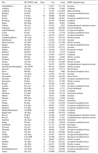
We used the 20 FLUXNET sites used in Best et al. (2015), plus an additional 41 high-quality sites, including 20 from the La Thuile FLUXNET release (Fluxdata, 2017) via the Protocol for the Analysis of Land Surface models (PALS), and another 21 from the OzFlux network (see Table 1). All data used in this study have a 30 min resolution.

We were interested in obtaining estimates for three land–atmosphere fluxes that are important for climate and weather prediction: latent heat (Qle), sensible heat (Qh), and net ecosystem exchange (NEE). While there are other fluxes that are relevant for climate modelling (runoff, for example), these are less well constrained by data. For the sake of fair comparison with LSMs, we corrected for energy budget closure at all sites where net radiation (Rnet) was available (all but six sites) by scaling Qh and Qle values by the average ($\frac{\text{Qh}+\text{Qle}}{\text{Rnet}}$) over each site record.

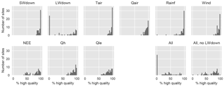
Figure 1 Histograms of percentage of high-quality data for each variable aggregated across all sites. The bottom right panels show the percentage of time steps that are high quality for the intersection of all of the variables at each site and the intersection of all variables except L.

We aimed to make use of all of the meteorological forcing variables that LSMs routinely use, including shortwave down (S), longwave down (L), air temperature (T), wind speed (W), rainfall (R), specific humidity (Q), and relative humidity (H). For the purposes of model training, we only used the high-quality periods of data, according to the quality-control flags provided in the La Thuile release, plus some quality control from the PALS project (detailed in Sect. 2a of Best et al., 2015). These flags remove periods of data that are clearly incorrect or synthesised. An overview of how much data are considered high quality for each variable across all sites is provided in Fig. 1. All quality-controlled data were used for training, so that data from sites with no high-quality data for longwave down, for example, were excluded from the training of models that include longwave down as a driver. However, all models still had substantial training data after low-quality data were excluded.

Although site characteristic data (for instance, soil and vegetation properties) are also likely to have significant effects on fluxes at a specific site, collection of these data at the site level is less standardised (for example, soil heat plate design and implementation differ substantially between different sites; see Sauer et al., 2003). Remotely sensed estimates are typically on much larger spatial scales than a flux tower's fetch (Chen et al., 2009) and have considerably larger uncertainties than in situ measurements. The data are also often discretised (e.g. by plant functional type) and thus cannot be used as a real-valued input to empirical models, effectively forcing models to provide separate parameterisations for each soil/vegetation combination.

By ignoring site characteristic data, and using meteorological variables only, we can set a lower bound on site predictability. Adding in accurate site characteristic data to empirical models should, conceptually at least, allow for improved empirical model performance, but as Best et al. (2015) and Haughton et al. (2016) showed, LSMs that already use these data do not perform better than simple empirical models based on meteorological data only.

The empirical benchmark models used in PLUMBER used only instantaneous meteorological driving data. However, the land surface has various storage pools for energy, water, and carbon. These storage pools effectively modulate the effect of meteorological forcing, modifying flux responses according to past meteorological information. While it would be possible to add state variables to an empirical model to represent these pools, without adding constraints, there would be a high risk of numerical instability. Such constraints would either have to come from conceptually based theory (making the models no longer purely empirical) or would have to be empirically calibrated, an extremely difficult task given the aforementioned numerical instability. An alternative approach is to assume that the historical record of a forcing variable has some impact and leave it to the empirical model to decide how to include that impact. We implemented this by calculating lagged averages of each variable, at varying time lags, and then used the variable selection process described below to pinpoint individually relevant lags.

The PLUMBER benchmarks had extremely simple structures. There are many potential empirical model structures that could be used to estimate an unknown functional relationship. While polynomial models, neural networks, and Gaussian process models can all fit arbitrary functions, these approaches often require either convoluted fitting processes (and thus are less desirable for broad-scale application to LSM benchmarking) and/or are likely to over-fit data for inexperienced users.

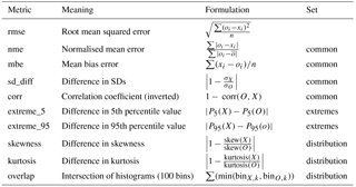
Table 2 Metrics used for performance assessment of model simulations. x indicates simulation values; o indicates observed values.

Best et al. (2015) used a cluster-plus-regression approach for the most complex of their models (3km27, a k-means clustering (k=27) with a linear regression at each cluster). This approach, originally from Abramowitz et al. (2010), is conceptually simple yet able to fit arbitrary functions simply by increasing the number of clusters. It is also computationally efficient, aside from the initial k-means clustering (which can be made more efficient via a number of optimisations). It does potentially have the problem of a prediction surface that is discontinuous at the edges of clusters (where several linear regressions meet), but we did not find this to be problematic. The k-means clustering is also somewhat dependent on its random cluster centre initialisation, which means that repeated k-means-based empirical models using the same training data result in slightly different outputs, but in our testing this variance only rarely affected ranks (see the Supplement for more details). In Best et al. (2015), the 3km27 model out-performed all LSMs for all fluxes when averaged across metrics and sites. We chose to continue to use this model structure here.

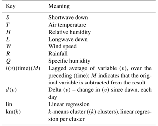
Table 3 Empirical model naming key. For example, a model named “STHWdT_lR10d_lT6hM_km243” has seven inputs (shortwave down, air temperature, relative humidity, wind speed, the difference in temperature between the current time step and dawn, 10-day lagged average of rainfall, and 6 h lagged average of air temperature minus instantaneous air temperature), and uses a 243-cluster k-means regression, with a separate linear regression of over all input variables for each cluster.

Following Best et al. (2015), all empirical models were tested out of sample only. They were trained using a leave-one-out strategy: for each site, they were trained on all of the other 60 sites and then given the meteorological data to run at the site in question. They were then evaluated using that site's flux measurements, which were not included in its training.

For all of our models, we use the Best et al. (2015) 3km27 (re-implemented and from here on labelled STH_km27; see naming scheme in Table 3) as a baseline from which to add complexity. The criterion for model selection in the final ensemble was simple – additional complexity must add predictive value to the model. Additional complexity can potentially degrade performance out of sample, due to increased risks of over-fitting (more parameters) or equifinality (essentially, getting the right answer for the wrong reason; see Medlyn et al., 2005). Where additional complexity did not substantially improve performance, we took an Ockham's razor approach – that is, where no clear distinction in performance is evident, prefer parsimony – and used the simpler model.

Other than choice of model structure, there are a number of ways that a model's complexity can increase. Firstly, using the same input and output variables, a model's internal structural complexity can be increased. In the case of cluster-plus-regression models, which are effectively a non-continuous piece-wise linear surface with one plane per cluster, this corresponds to using more clusters. Since the number of clusters defines the number of gradient discontinuities in the model, and hence its ability to fit more complex functions, we refer to this as the model's “articulation”. The input data are not inherently strongly clustered and so the number of clusters chosen is largely subjective. The Best et al. (2015) STH_km27 model was designed such that it could potentially divide the input space of three variables into three distinct regions in each dimension (hence, k=3³). In this study, we chose to continue this conceptual approach and look at models with k=243, 729, and 2187 (3⁵, 3⁶, and 3⁷ for 5, 6, and 7 input variables, respectively). This design continues to allow sufficient articulation in each variable dimension as more variables are added, i.e. for 243 clusters, five input variable domains could each be split into three bins, independent of the other variables. In practice, however, the clusters are not distinct in each individual variable domain – they each generally have some overlap. The articulation over one variable conditional on other variables may therefore be higher or lower. It is also worth noting that a model with more input variables effectively has less articulation per variable than a model with fewer variables but the same number of clusters.

Another obvious method of increasing complexity is to add extra predictor variables. Starting from STH_km27, we can add in any of the remaining variables (L, W, R; see Table 3). We also noted that Gentine et al. (2016) identified two key meteorological variable transformations as highly predictive for heat fluxes, namely change in T since dawn (delta T) and change in Q since the previous sunrise (delta Q). We included both of these transformations as additional predictors, using the first time step with ≥ 5 W m⁻² S as our “dawn” reference point.

For each predictor variable not included in the original PLUMBER study, we generated variants of the original STH_km27 that included each variable, one at a time, for k=27 and 243 (e.g. STHL_km27, STHL_km243). These were compared to the results from the original PLUMBER models (S_lin, ST_lin, STH_km27) as well as an increased-articulation variant with only the original three PLUMBER variables (STH_243) to ensure that each new variable was actually adding predictive power. Since adding in extra variables increases the dimensionality of the input space, we might expect increased articulation to have more impact.

Thirdly, we can add in some historical variant of any of the input variables. For each variable, we used varying time periods and calculated the average of the preceding period for each time step (excluding the time step itself; e.g. since all data were half hourly, for the 2 h lagged average, we calculated the average of the previous four time steps). The averages we used were 30 min, 1, 2, 6, 12 h, 1, 2, 7, 10, 30, 60, 90, and 180 days. We then compared the set of models with added lagged averages for a given variable to each other, as well as the original three Best et al. (2015) benchmarks. This allowed us to identify which variants of the lagged variables were adding the most value. Lagged correlation plots are shown for each variable in the Supplement and give an a priori indication of which lags for different variables might add additional information to an empirical model.

Variables also have interacting responses; for example, two variables might have a multiplicative flux response. It is theoretically possible to generate models that cover all the possible interactions between variables. However, even if we only included a handful of instantaneous variables and a handful of possible interactions, the set of models to run would quickly become impossibly large. Fortunately, the articulation that the cluster-plus-regression model structure allows for can approximately fit any such interaction without the need to actually include the interaction terms in the regressions.

To ensure that any variables identified as providing additional predictive power did not interact in problematic ways (e.g. collinearity), we investigated the pair-wise correlations between each variable. Given that the system has significant non-linearities, this is not a perfect method of ensuring lack of collinearity. However, as a first approximation, it allows us to remove any obviously pair-wise-correlated variables.

Once we had identified the key variables that provided substantial performance increases, we generated an small hierarchically defined ensemble of models using these variables. The ensemble is designed to be a conceptually simple set of benchmarks that can be used by other researchers in model evaluation and development. The ensemble includes the original three PLUMBER benchmarks and several other models of gradually increasing in complexity. We use this model ensemble to reanalyse the LSM results from the original PLUMBER experiment.

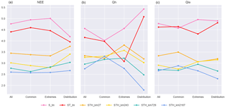
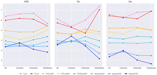
Figure 2 Rank-average plots of empirical models using the same inputs as STH_km27, with an increasing number of clusters. Metrics (Table 2) are calculated for each flux variable for each model simulation at each of the 61 FLUXNET sites, and in each case models are ranked. The first column of values in each panel represents the rank average over all sites and all 10 metrics, the second column all sites and “common” metrics (NME, MBE, SD_diff, correlation), the third column all sites and the two extremes metrics (extreme_5, extreme_95), and the fourth column all sites and the distribution-related metrics (skewness, kurtosis, overlap). Lower values indicate better overall performance, and lines only serve to visually connect data points (gradients are irrelevant).

3 Results

As a first step, we investigated how much value additional articulation would add to the STH_km27 model by comparing it to models with the same inputs and structure but using 243, 729, and 2187 clusters (Fig. 2). This and subsequent figures use the same methodology as Figs. 4–6 in Best et al. (2015). They show the performance rank of each model, relative to other models in the plot, for each flux variable averaged over the 61 FLUXNET sites and over 10 different performance metrics (listed in Table 2). In this and the following similar plots, a lower rank average is better and should be interpreted as a model performing better than a higher model more often than not. The larger the difference, the more often the lower-ranked model wins. The differences in the y values in these plots do not necessarily indicate how much better a model performs than other models, although analysis in Haughton et al. (2016) indicates that ranks do tend to approximate relative performance values when assessed in aggregate.

In Fig. 2, the three panels show the rank-average results for each of the models over the three flux variables relative to each other. The first column of each panel represents the averages across all sites and all metrics, the second column averages only over the common metrics, third column only over the extremes metrics, and the fourth column only the distribution-related metrics (see figure caption for details). At the most general level, with performance averaged over all metrics (first column of each panel), the STH_km243 model (yellow) provides substantial improvement over STH_km27 for Qle and NEE. There does not appear to be any improvement for Qh. STH_km729 appears to provide a slight further improvement for all three fluxes. STH_km2187 provides minor and probably negligible improvement over STH_km729 for all fluxes, with the possible exception of extremes and distribution metrics for Qh and Qle. Examining the results separately over the different metric sets used in Best et al. (2015) (columns 2, 3, and 4 in each panel), the models with more articulation substantially improve the performance of the prediction of extremes for NEE, and both extremes and distributions for Qh and Qle. Articulation beyond 729 clusters offers no additional benefit for the common metrics. ST_lin does exceptionally well for Qh prediction under the extremes, relative to all but the highest cluster-count non-linear model. We note that this is the most volatile category due to the sensitivity of empirical models to outliers affecting the extremes, and because this group only contains two metrics. Increased articulation is more likely to provide more benefit with more input variables, but using more variables also increases the likelihood of both incomplete time steps (as any given variable might have a low-quality data point) and of the clustering algorithm failing to converge (e.g. some clusters may not be assigned a value, causing the model to crash). We did some further testing of 2187 clusters in later parts of the study, but since these models crashed more frequently, and did not obviously add further performance improvement, we excluded them from the remainder of the paper.

Next, we tested which of the additional available meteorological forcing variables added value to the models. We tested L, W, and R (we omitted Q, as this information is already largely contained in the T and H variables), as well as delta Q and delta T. For each variable, we created km27 and km243 variants, and compared them to the original PLUMBER benchmarks (S_lin, ST_lin, STH_km27), plus STH_km243.

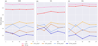
Figure 3 Models with a single additional variable. As per Fig. 2, except that each column includes four baseline benchmark models (S_lin, ST_lin, STH_km27, and STH_km243), plus STHX_km27 and STHX_km243, versions of STH_km27 and STH_km243 with an extra instantaneous meteorological or derived variable included as an input (variables are listed along the x axis, models with added variables are in blue shades). All points are rank averages over all sites and all metrics.

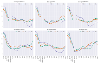
Figure 4 Models with a single additional lagged average meteorological variable input. The five leftmost models (columns) in each panel are for reference; other models represent STH_lxxx_km243, where xxx is the time average over the lag period (specified on the horizontal axis) of the variable shown in each panel (e.g. S for panel a). Vertical axes show the average rank average of each of the models (on the x axis) against all other models in the panel.

Figure 3 shows that instantaneous W provides substantial benefits for model prediction for all fluxes at both 27 and 243 clusters. Instantaneous L appears to provide substantial benefit for Qle prediction but does not clearly improve the performance of Qh or NEE fluxes. Instantaneous R appears to slightly degrade performance across all fluxes at both cluster counts. Delta Q provides substantial improvement for Qle prediction, and some improvement for Qh, but the impact on NEE performance is a negligible degradation of performance. Delta T also provides some improvement for Qle and NEE, and does not clearly improve Qh prediction.

Even if the additional variables do not add substantially to the performance of the models, lagged averages of those variables might. We additionally tested model variants with lagged averages of each meteorological variable. Figure 4 shows that despite instantaneous S, T, and H already being in the reference models, lagged averages of these variables appear to offer additional predictive ability. Longer lags of S and H help the prediction of Qle, perhaps because these variables act as proxies for soil moisture, ground heat storage, or boundary layer dynamics (e.g. Gentine et al., 2016). Both 2 and 6 h lags of T appear to provide a performance improvement, but these lags likely also correlate highly with instantaneous T (see the Supplement). Models with lagged averages of L and W do not appear to provide any benefit over the instantaneous variables and appear to degrade performance substantially for longer lags. Short lags of R appear to substantially decrease the performance of models for all fluxes; however, longer lags appear to provide some benefit, especially for Qle (10–90 days).

From the above investigations, we determined that there were eight key variables in addition to the three already used in the PLUMBER benchmark models. The entire set of relevant variables is instantaneous S, T, H, and wind; delta T; delta Q; and lagged average variants of T (6 h), S (30 days), R (30 days), and H (10 days). In some cases, there were multiple lags with similar overall performance gains. For these, we chose one by selecting the variant that gave the best compromise performance increase between the three fluxes, as well as preferring lags towards the middle of the spectrum, so as to avoid correlation with instantaneous variables and to maximise the available training data (longer lags mean fewer windows with complete data available). To ensure minimal likelihood of problems with collinearity of forcing variables, we calculated the pair-wise correlations between each pair of potential forcing variables and the fluxes. For this investigation, we removed all low-quality data across all selected variables, which resulted in the AdelaideRiver site being remove due to it having no controlled rainfall data. This left over 1.6 million time steps of data.

Figure 5 Pair-wise correlations between forcing variables and fluxes.

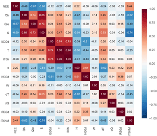
Figure 5 shows that the three fluxes are fairly highly correlated with one another and with S. This was already indicated by the good performance of the 1lin benchmark in PLUMBER. Of the other individual driving variables, T, H, and delta T have the next highest correlations with the fluxes. The first two of these were also indicated by the performance of 3km27 in PLUMBER. Delta T also has high correlations with S, T, and H. However, a multiple linear regression on these three variables only has an R² value of 0.66, indicating that there is still substantial independent information in this variable that may be of use to empirical models. There are also very high correlations between the 30-day lagged average of S, instantaneous T, and the 6 h lagged average T. In particular, the regression of 6 h lagged average T on instantaneous T has an slope coefficient of 0.9992 and an R² value > 0.999. This is because the lagged average still contains all of the annual cycle information and all of the daily cycle information (albeit out of phase by 3 h). However, the lagged average does not contain any of the high-frequency information, and because of the lag it effectively gives the model a time-of-day proxy. To overcome the correlation problem, we added a lagged average minus instantaneous variant (last row/column in Fig. 5), which avoided the high correlation with 30-day averaged S and instantaneous T. This variable has a relative high correlation with instantaneous S but still contains substantial independent information (R² of 0.41 for a regression on S).

Next, we combined our approach to generate a set of models that uses the informative variables identified above. To create a set of models that spans a range of performance and behaviours, we generated all combinations of the model with a selected set of input variables, according to the results of previous sections. In addition to the three variables used in the original PLUMBER empirical models (S, T, and H), these variables were instantaneous wind, delta T, delta Q, and lagged average variants of S (30 days), R (30 days), H (10 days), and T (6 h, with instantaneous values subtracted). Each variable was chosen for its ability to improve the performance of the models substantially for at least two of the three fluxes. Initially, we also included L in the models, but we found that this appeared to substantially decrease performance of models (in some cases so much that these models were outperformed by S_lin). This may be due to the low quality of L in the datasets and complete lack of L in over a third of sites (see Fig. 1), which would minimise the data available both for training as well as for evaluation. Therefore, we decided to remove L as a candidate driving variable. In the case of the lagged variables, there was the added concern that long lags (> ∼ 30 days) would decrease the performance over shorter datasets (the models use the long-term average when not enough data are available to calculate the lags) and that short lags (< 1–2 days) would have a high correlation with instantaneous variables (only relevant when the instantaneous variables were also included).

We aimed to generate an objectively “best” ensemble that evenly spanned the range of performance in each variable, and maximised behavioural diversity. For example, we might expect that models with instantaneous humidity would exhibit different patterns in their outputs after a rain event than models that do not include humidity. Likewise, models with lagged rainfall averages as drivers should also have a differing behaviour in the period after a rainfall event.

We initially attempted a pseudo-optimisation-based ensemble generation approach. This consisted of first generating models for all possible combinations of the seven variables identified above at 243- and 729-cluster counts. Then, starting with the three PLUMBER benchmarks and the best performing of these model for each flux, we sequentially added in the models that were most independent from the existing models in the ensemble by selecting the models with the lowest average error correlation with the models already selected. This resulted in ensembles quite similar in performance to the ensemble described below but with less well-defined conceptual structure. Therefore, we decided to manually create an ensemble from a conceptual classification of the input variables.

Of the newly identified variables there are three clear groupings. Firstly, W is the only instantaneous variable that adds substantially to the performance of models. The second group is the three variables that only include short-term information: delta T, delta Q, and the 6 h lagged average of T. These variables likely provide proxies for short timescale states in the system (e.g. within-canopy heat and surface water). The last group is the three variables that include long-term information: the 30-day averages for S and R, and the 10-day average for H. These variables provide information about long timescale states in the system, such as ground heat, soil moisture, and perhaps leaf area index.

Figure 6 Rank-average plot of the eight models in the final ensemble.

We decided to create models that gradually increased in complexity by first adding further articulation to the PLUMBER models and then gradually adding in these variable groupings. In doing so, we noted that the 243-cluster variants more often out-performed the 729-cluster variants in the common metrics, while the 729 variants tended to perform better in the extremes and distribution metrics. As such, we decided to include models starting with the three PLUMBER benchmarks, then a model with further articulation, then a model with the relevant instantaneous variable (wind), then a model with the short-term information, and then a model with the long-term information. We also added both the 243- and 729-cluster variants of the most complex model. This model is most likely to benefit from a higher cluster count because it has more driving variables. The two variants display quite different behaviour. This left us with this final ensemble (short names in parentheses):

• S_lin,

• ST_lin,

• STH_km27,

• STH_km243,

• STHW_km243,

• STHWdTdQ_lT6hM_km243 (short_term243),

• STHWdTdQ_lT6hM_lS30d_lR30d_lH10d_km243 (long_term243), and

• STHWdTdQ_lT6hM_lS30d_lR30d_lH10d_km729 (long_term243).

The selected set spans a broad range of performance in each of the three fluxes and includes multiple modes of increased complexity (increasing articulation, added variables, lagged variables). The relative performance of these models is shown in Fig. 6. The three original empirical models in PLUMBER are consistently out-performed across variables and the more complex models tend to out-perform less complex models. There are some notable exceptions to this. The performance in the most complex models is reduced under the common metrics, especially for Qh. The performance of the increased articulation model (STH_km243, yellow) is also reduced relative to the simpler model with the same inputs (STH_km27, orange) under the common metrics for Qh, and the distribution and extremes metrics for Qle. As in Fig. 2, the two-variable linear model performs well against the next most complex models for NEE under the distribution metrics and relatively well for the Qh extremes metrics.

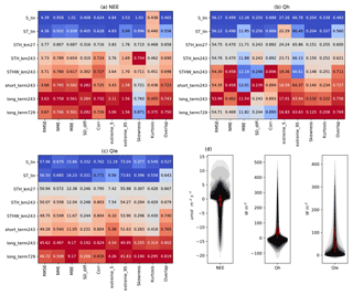
Figure 7 The three matrix panels (a–c) show metric values averaged over all sites. All models are compared to STH_km27 as a baseline (grey), better models are shown in red, and worse models in blue, where dark red/blue indicates the best/worst model in ensemble, for each metric independently. The fourth panel (d) shows observed distributions of each flux, trimmed at the 5th and 95th percentiles, plotted independently for each site and overlaid at 10 % opacity. The red box plots show the distribution of site means for each flux, with whiskers extending to 1.5 times the interquartile range, and outlying sites shown beyond as points.

These data are shown again in Fig. 7a–c, this time with more emphasis on individual metrics, and how they change as models become more complex. In many cases, there is a clear graduation from the simplest model performing worst (blue) to the most complex model performing best (red; e.g. the pdf overlap metric for all fluxes). Some metrics, however, clearly degrade with complexity, such as skewness for NEE where performance appears to degrade further as more variables are added. Some of the less consistently improving metrics (e.g. MBE, SD_diff, Corr, and Extreme95 for Qh) are due to the fact that these metrics only change by about 5 % between the worst and best models (< 1 % for Corr), and so noise in the metric results may dominate any trend. In general, however, there is a consistent gradation of performances across the model ensemble. Figure 7d shows the distributions of the energy-closure-corrected observed site fluxes, plotted and overlaid for each site, for comparison with value-dependent metrics.

There is inevitable subjectivity in choosing an ensemble such as this, given the infinite number of possible model structures. This ensemble strikes a balance between selecting a diverse range of performance and behaviours and maintaining a clear conceptual hierarchy. The three forcing variable groupings (instantaneous, short-term, and long-term) also potentially provide a way to understand how much performance improvement different model state variables should provide and thus help to identify which model process representations might require improvement.

Having explored FLUXNET datasets for key forcing variables relevant for flux prediction, as well as the longer-term information contained in those variables, and having created a conceptually coherent benchmark ensemble, we now put the ensemble to use in an LSM intercomparison.

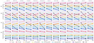
Figure 8 Comparison of the final ensemble to the PLUMBER LSMs. Each panel compares a single LSM (in black, different in each column) with all seven empirical benchmarks (coloured as per Fig. 6), and each column within the panels represents a single flux variable, similar to the design of the plots in Best et al. (2015). The first row (a) shows the average rank over all 10 metrics listed in Table 2. The second, third, and fourth rows (b–d) show the metric groups used in, e.g. Fig. 6. The second, third, and fourth rows correspond to Figs. 4–6 in Best et al. (2015).

Land surface model evaluation

We compare the ensemble selected above with the LSM simulations used in Best et al. (2015), continuing the work from Haughton et al. (2016). Figure 8 shows a recreation of the key figures from Best et al. (2015) using our empirical benchmarks. NEE is omitted from this figure for ease of comparison with the original Best et al. (2015) figures (see figure caption) and because NEE is only included in the output of 4 of the 13 LSMs.

In the second row, we still see the pattern shown by Best et al. (2015) for Qh, that the LSMs are all consistently beaten by even the simplest empirical models (LSMs in black are consistently above S_lin in pink and ST_lin in red). However, in our version, for Qle, the LSMs appear to be doing relatively better, beating STH_km27 consistently. This is for a number of reasons. Firstly, the empirical models in this study are trained on more sites than the Best et al. (2015) empirical models, and this may cause some differences, particularly with the cluster-and-regression model variants, which are sensitive to initialisation of the k-means clusters (see the Supplement). Secondly, all site data used in this version of the figure are energy-closure corrected which improves LSM rankings in some cases. This is similar to Fig. 8 in Haughton et al. (2016), but the closure is dealt with differently. The analyses undertaken here also only use the quality-controlled data for each site in contrast with Best et al. (2015) and Haughton et al. (2016) which used all data. Thirdly, if the empirical models tend to cluster around certain values for a particular metric, then it is more likely that if an LSM beats STH_km27 it will beat many of the empirical models and therefore skew the overall rank average towards a lower value. This is the case for SD_diff in particular as can be seen for Qle in Fig. 10. This is perhaps to be expected as the empirical benchmarks are smoothers, only adding variance from the meteorological forcings (this was also shown in Fig. 4 in Haughton et al., 2016). This effect is potentially even more pronounced in the absence of the physical benchmarks used in Best et al. (2015) and Haughton et al. (2016). Despite this latter effect, we still see the LSMs generally falling in the middle of the range of empirical models for Qle under the common metrics. This indicates that our newer and more complex benchmarks are adding substantial non-spurious performance improvements over the PLUMBER benchmarks.

In the third row of Fig. 8, aside from a few cases (in particular COLASSiB2), the LSMs generally perform better under the extremes metrics. Indeed many of the LSMs beat all of the empirical models for Qle and at least fall in the middle of the range of performances for Qh. This is quite similar to the results shown in Fig. 5 in Best et al. (2015) where the LSMs generally performed similarly to the most complex benchmark, 3km27. Under the distribution metrics (fourth row), the LSMs generally perform better than all but the most complex of the empirical models. This corresponds reasonably well with Fig. 6 in Best et al. (2015). It is notable here, as in Best et al. (2015), that the LSMs perform reasonably well under Qle relative to the other two fluxes. The three fluxes operate very differently, and so it is not clear why this performance difference exists, but it may be due to, e.g. tighter constraints on Qle from upper-level soil moisture (which is not available to the empirical models), or it may be that the boundary layer turbulence affects Qle less strongly than the other fluxes.

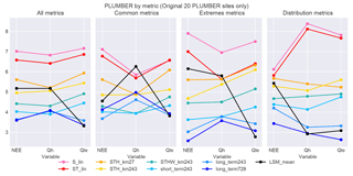
Figure 9 Rank-average plots, including the PLUMBER LSM ensemble mean by metric group: in this plot, the black line represents the unweighted mean of all 13 PLUMBER model simulations at a given site and variable. Note that the NEE results are the mean of only the four models that included NEE in their output.

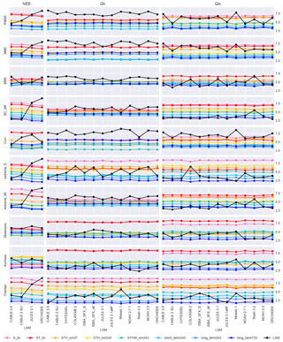
Figure 10 PLUMBER LSMs by metric: this figure shows the average ranks of models over all 20 sites and allows easier side-by-side comparison between LSMs. Each row contains only a single metric and each column of plots a single flux variable, with LSMs on the x axis. Flux values for the empirical benchmarks are identical along the x axis for each panel, but ranks change due to relative differences between LSMs.

We also examine the performance of the mean of the 13 LSMs in PLUMBER (Fig. 9) against our new empirical model ensemble (similar to Fig. 12 in Haughton et al., 2016). In the first panel, we see that the mean performs substantially better under all metrics for Qle than nearly all individual models but substantially worse for Qh (first row in Fig. 8). The LSM mean is competitive with the most complex empirical benchmarks for Qle under all four metrics sets, out-performing all of the benchmarks under all metrics and the extremes metrics. NEE performance of the mean falls toward the middle of the range of the benchmarks under all four metric sets. The LSM mean performs substantially worse than most benchmarks for Qh, except under the distribution metrics, where it out-performs all benchmark models.

It is also instructive to examine these data through other lenses. The original PLUMBER results compared LSMs averaged over sites and metrics for multiple variables at once. One could alternatively compare LSMs over only a single variable at once, as per earlier figures in this paper. Figure 10 compares models over a single variable in each major column and over a single metric in each row, with each point representing the relative rank over all 20 sites. While it represents the same data shown in Fig. 8, it is perhaps a more straightforward intercomparison between LSMs than the original Best et al. (2015) figures. In particular, it becomes clear under which metrics the models are collectively performing poorly for Qh (RMSE, NME, Corr, extreme_95) and that performances for Qle are perhaps more heterogeneous than might be interpreted from Fig. 8. It also highlights that some models stand out as poor performers in particular circumstances (e.g. MOSAIC for RMSE, Noah 3.2 for MBE, and COLASSiB for extreme_5). It is difficult to assess the relative performances of the LSMs for NEE due to the small group size. However, it is clear that the CABLE variants out-perform JULES and ORCHIDEE for NEE under RMSE, NME, SD_diff, and the extremes metrics.

4 Discussion

We have shown that empirical model performance can be improved substantially over the benchmarks used in PLUMBER using meteorological data alone. This is true for all three fluxes under investigation and across multiple sets of performance metrics. Although we used models capable of fitting arbitrary function surfaces, it is probable that more information could be extracted from the FLUXNET meteorological forcings and allow even higher predictability given enough training data. For example, there may be better ways to include information from the historical time series of each forcing variable than just using lagged averages.

There is also no doubt that performance could be further increased using similar models with additional site characteristic data, such as soil composition, vegetation structure, and orography. This is a much more complex problem as noted in the introduction. While we ruled out a number of meteorological variables and derived variants in our models, it is possible – should suitable site data be made available during model training – that these variables might be more relevant if they have dependent interactions with those site variables.

This current empirical model ensemble provides a set of a priori lower bounds on the information available in the meteorological forcings for predicting fluxes. The ensemble also provides a number of intermediate complexity estimates for instances where less data are available or of interest. In particular, the values in Fig. 7 can be used as a benchmark for LSMs in other studies and the hierarchy of model complexity can give an idea of the spread of metrics that might be expected. It could also predict how much a metric should be expected to improve as a model is supplied with more information. We hope that this ensemble might be used among the land surface modelling community as a common reference point and that it might pave the way to the creation of a benchmarking standard. As such, we have provided the code required to reproduce the benchmarks on appropriate data (with slight variation, as noted in the Supplement).

If conceptually simple empirical models are already comprehensively out-performing physically informed LSMs and can presumably be improved upon with additional site characteristic data, then the following question arises: why bother with physically based models? One argument is that empirical models will only predict well in environments that are similar to their training environments. For example, they may not predict well in a world with raised CO₂ levels. However, we now have tower-based measurements of a broad spectrum of environments – much broader than the change at any particular location expected over the next century (Pitman and Abramowitz, 2005) – so it is not unreasonable to expect empirical models to perform reasonably well for some range outside the norm. It is worth noting that empirical models of complex systems are necessarily simplifications, and as a consequence, even when they may adequately model the aggregate behaviour, they are likely to miss important behaviours that arise from the complex interactions within the system (Batty and Torrens, 2001). On the other hand, LSMs report a range of other variables aside from fluxes that are key to coupled modelling systems (e.g. runoff) and impact assessments (e.g. soil moisture and temperature). They also have one major benefit over empirical models: their parameters have a physical meaning and can be manipulated to learn about changes in the behaviour of the system. However, this is only true if those parameters are representative of something real, if they are constrained adequately by data, and if the model's components interact realistically. A hybrid approach of empirical model components constrained by available data and conservation principles remains a possibility for future work.

In general, numerical LSMs have become increasingly complex over the last 5 decades, expanding from basic bucket schemes to models that include tens or even hundreds of processes involving multiple components of the soil, biosphere, and within-canopy atmosphere. Model components may have been added on to existing models without adequate constraint on component parameters (Abramowitz, 2013) or without adequate system closure (Batty and Torrens, 2001). New component parameters may be calibrated against existing model components, leading to problems of equifinality (Medlyn et al., 2005), non-identifiability (Kavetski and Clark, 2011), and epistemological holism (Lenhard and Winsberg, 2010). These problems can often only be overcome by ensuring that each component is itself well constrained by data and numerically stable (Kavetski and Clark, 2011). As noted earlier, these conditions rarely exist for any given component.

While appropriate use of available data is a prerequisite to model generation, it is not sufficient by itself. Over-reliance on data could lead to underestimation of uncertainty, where systematic errors in the data are not accounted for. Data can be used to inform model development, but they should not be used alone to drive model development: “Data is a valuable adviser but a tyrannical master” (Bowles, 2016). Over-reliance on data could lead to poor decision making when expertise is ignored in favour of data-driven approaches that ignore aspects of the environment outside of the scope of the dataset. Even assuming no systematic errors in the data and an appropriate model structure, model results must still be interpreted. This requires significant experience on the part of the researcher. However, as long as they are not over-fitted, we can use naive empirical models as benchmarks, as prior distributions for the prediction performance of LSMs (as demonstrated by Nearing and Gupta, 2015), wherever adequate data exist.

The empirical model ensemble outlined in this paper is relatively easy to reproduce on any land surface data. It may be used by LSM developers as a tool for identifying situations in which their model is performing inadequately. For example, if empirical models are performing significantly better than an LSM at a particular subset of sites or at a particular time of year or day, this difference could be used to help identify environments in which the LSM could improve. The diversity of models in the ensemble could also help highlight which components of an LSM might be targeted for improvement. For example, if the models with W included as a driving variable are performing substantially better than the models without W in a particular situation, that may indicate that there are problems with the LSM's handling of surface evaporation. Alternatively, if the model with lagged R is performing better than other models over a dry period, that may indicate that soil moisture might be a key factor in behaviour of the fluxes over that period.

5 Conclusion

We have attempted to set lower bounds on the predictability of surface fluxes and have shown that using only meteorological driving data empirical model performance in previous studies can be improved by adding further complexity. This study used only meteorological data to predict fluxes and as such does not attempt to quantify the relevance of various important site characteristic variables, including soil, vegetation, or orography. As records of these types of variables become more standardised, the methodology used here may be extended to include them.

This study provides an ensemble of empirical models spanning a broad range of performance and behaviour that can be used as a standard set of benchmarks for LSM evaluation. The conceptual structure of the ensemble also illustrated the degree to which predictability is derived from instantaneous, short-term, or long-term information. The ensemble is relatively easy to reproduce and may be used by LSM developers as a tool for identifying situations in which their model is performing inadequately.

We have also shown that LSMs, while still clearly performing less well than we might hope, are performing substantially less homogeneously than might have been expected from Best et al. (2015) or Haughton et al. (2016). Actually attributing poor LSM performance to particular aspects of those models remains elusive, but we hope that the benchmark ensemble presented here will allow for more nuanced evaluation of LSMs in the near future.