the Creative Commons Attribution 4.0 License.
the Creative Commons Attribution 4.0 License.
 | 02 May 2018
Near-global climate simulation at 1 km resolution: establishing a performance baseline on 4888 GPUs with COSMO 5.0
Oliver Fuhrer
Tarun Chadha
Torsten Hoefler
Grzegorz Kwasniewski
Xavier Lapillonne
David Leutwyler
Daniel Lüthi
Carlos Osuna
Christoph Schär
Thomas C. Schulthess
Hannes Vogt
The best hope for reducing long-standing global climate model biases is by increasing resolution to the kilometer scale. Here we present results from an ultrahigh-resolution non-hydrostatic climate model for a near-global setup running on the full Piz Daint supercomputer on 4888 GPUs (graphics processing units). The dynamical core of the model has been completely rewritten using a domain-specific language (DSL) for performance portability across different hardware architectures. Physical parameterizations and diagnostics have been ported using compiler directives. To our knowledge this represents the first complete atmospheric model being run entirely on accelerators on this scale. At a grid spacing of 930 m (1.9 km), we achieve a simulation throughput of 0.043 (0.23) simulated years per day and an energy consumption of 596 MWh per simulated year. Furthermore, we propose a new memory usage efficiency (MUE) metric that considers how efficiently the memory bandwidth – the dominant bottleneck of climate codes – is being used.
- Article
(3578 KB) - Full-text XML
- BibTeX
- EndNote


Should global warming occur at the upper end of the range of current projections, the local impacts of unmitigated climate change would be dramatic. Particular concerns relate to the projected sea-level rise, increases in the incidence of extreme events such as heat waves and floods, and changes in the availability of water resources and the occurrence of droughts (Pachauri and Meyer, 2014).
Current climate projections are mostly based on global climate models (GCMs). These models represent the coupled atmosphere–ocean–land system and integrate the governing equations, for instance, for a set of prescribed emissions scenarios. Despite significant progress during the last decades, uncertainties are still large. For example, current estimates of the equilibrium global mean surface warming for doubled greenhouse gas concentrations range between 1.5 and 4.5 ∘C (Pachauri and Meyer, 2014). On regional scales and in terms of the hydrological cycle, the uncertainties are even larger. Reducing the uncertainties of climate change projections, in order to make optimal mitigation and adaptation decisions, is thus urgent and has a tremendous economic value (Hope, 2015).
How can the uncertainties of climate projections be reduced? There is overwhelming evidence from the literature that the leading cause of uncertainty is the representation of clouds, largely due to their influence upon the reflection of incoming solar radiation (Boucher et al., 2013; Bony et al., 2015; Schneider et al., 2017). Horizontal resolutions of current global climate models are typically in the range of 50–200 km. At this resolution, clouds must be parametrized, based on theoretical and semiempirical considerations. Refining the resolution to the kilometer scale would allow the explicit representation of deep convective clouds (thunderstorms and rain showers; e.g., Fig. 1). Studies using regional climate models demonstrate that at this resolution, the representation of precipitation is dramatically improved (Kendon et al., 2014; Ban et al., 2015). The representation of shallow cumulus cloud layers, which are common over significant fractions of the tropical oceans, requires even higher resolution. The United States National academy of sciences has thus recommended (Natinal Research Council, 2012) developing “high-end global models that execute efficiently ... , enabling cloud-resolving atmospheric resolutions (2–4 km) and eddy-resolving ocean resolutions (5 km)” in the near future.
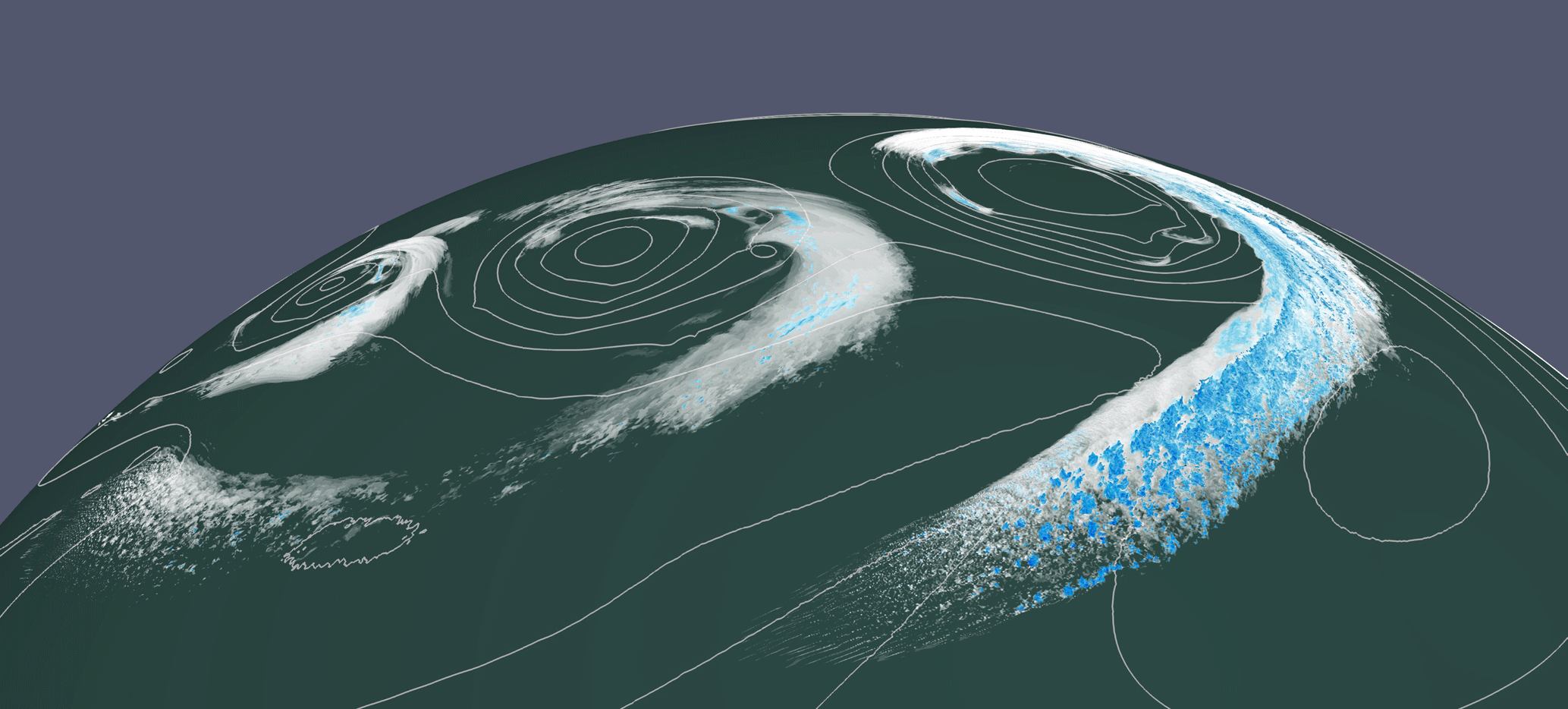
Figure 1Visualization of a baroclinic wave at day 10 of a simulation with 930 m grid spacing. White shading: volume rendering of cloud ice, cloud water, and graupel g kg−1. Blue shading: isosurface of rain and snow hydrometeors g kg−1. The white contours denote surface pressure.
While the scientific prospects of such an undertaking are highly promising, the computational implications are significant. Increasing the horizontal resolution from 50 to 2 km increases the computational effort by at least a factor of 253=15 000. Such simulations will only be possible on future extreme-scale high-performance computers. Furthermore, power constraints have been driving the widespread adoption of many-core accelerators in leading edge supercomputers and the weather and climate community is struggling to migrate the large existing codes to these architectures and use them efficiently.
But what does efficient mean? While concerns of the total cost of ownership of a high-performance computing (HPC) system have shifted the focus from peak floating point performance towards improving power efficiency, it is not clear what the right efficiency metric is for a fully fledged climate model. Today, floating point operations are around 100× cheaper than data movement in terms of time and 1000× cheaper in terms of energy, depending on where the data come from (Borkar and Chien, 2011; Shalf et al., 2011). Thus, while focusing on floating point operations was very relevant 25 years ago, it has lost most of this relevance today. Instead, domain-specific metrics may be much more applicable to evaluate and compare application performance. A metric often used for climate models is the throughput achieved by the simulation measured in simulated years per wall clock day (SYPD; see Balaji et al. (2017) for a detailed discussion on metrics). For global atmospheric models, a suitable near-term target is to conduct decade-long simulations and to participate in the Atmospheric Model Intercomparison Project (AMIP) effort. 1 Such simulations require a 36-year long simulation for the period 1979–2014, driven by observed atmospheric greenhouse gas concentrations and sea-surface temperatures. Within the context of current climate modeling centers, such a simulation would be feasible for an SYPD greater than or equal to 0.2–0.3. At such a rate the simulation would take up to several months. However, domain-specific metrics such as SYPD are very dependent on the specific problem and approximations in the code under consideration and are often hard to compare. Ideally comparisons would be performed for production-quality global atmospheric models that have been extensively validated for climate simulations and cover the full (non-hydrostatic and compressible) dynamics and the entire suite of model parameterizations.
With the SYPD metric alone, it is hard to assess how efficiently a particular computing platform is used. Efficiency of use is particularly important because, on the typical scale of climate simulations, computing resources are very costly and energy intensive. Thus, running high-resolution climate simulations also faces a significant computer science problem when it comes to computational efficiency. As mentioned before, floating point efficiency is often not relevant for state-of-the-art climate codes. Not only does counting floating point operations per second (flop s−1) not reflect the actual (energy) costs well, but the typical climate code has very low arithmetic intensity (the ratio of floating point operations to consumed memory bandwidth). Attempts to increase the arithmetic intensity may increase the floating point rate, but it is not clear if it improves any of the significant metrics (e.g., SYPD). However, solely focusing on memory bandwidth can also be misleading. Thus, we propose memory usage efficiency (MUE), a new metric that considers the efficiency of the code's implementation with respect to input/output (I/O) complexity bounds as well as the achieved system memory bandwidth.
In summary, the next grand challenge of climate modeling is refining the grid spacing of the production model codes to the kilometer scale, as it will allow addressing long-standing open questions and uncertainties on the impact of anthropogenic effects on the future of our planet. Here, we address this great challenge and demonstrate the first simulation of a production-level atmospheric model, delivering 0.23 (0.043) SYPD at a grid spacing of 1.9 km (930 m), sufficient for AMIP-type simulations. Further, we evaluate the efficiency of these simulations using a new memory usage efficiency metric.
Performing global kilometer-scale climate simulations is an ambitious goal (Palmer, 2014), but a few kilometer-scale landmark simulations have already been performed. While arguably not the most relevant metric, many of the studies have reported sustained floating point performance. In 2007, Miura et al. (2007) performed a week-long simulation with a horizontal grid spacing of 3.5 km with the Nonhydrostatic Icosahedral Atmospheric Model (NICAM) on the Earth Simulator, and in 2013 Miyamoto et al. (2013) performed a 12 h long simulation at a grid spacing of 870 m on the K computer, achieving 230 Tflop s−1 double-precision performance.2 In 2014, Skamarock et al. (2014) performed a 20-day long simulation with a horizontal grid spacing of 3 km with the Model for Prediction Across Scales (MPAS) and later, in 2015, participated in the Next Generation Global Prediction System (NGGPS) model intercomparison project (Michalakes et al., 2015) at the same resolution and achieved 0.16 SYPD on the full National Energy Research Scientific Computing Center (NERSC) Edison system. In 2015, Bretherton and Khairoutdinov (2015) simulated several months of an extended aquaplanet channel at a grid spacing of 4 km using the System for Atmospheric Modeling (SAM). Yashiro et al. (2016) were the first to deploy a weather code on the TSUBAME system accelerated using graphics processing units (GPUs). The fully rewritten NICAM model sustained a double-precision performance of 60 Tflop s−1 on 2560 GPUs of the TSUBAME 2.5 supercomputer. In 2016, Yang et al. (2016a) implemented a fully implicit dynamical core at 488 m grid spacing in a β-plane channel achieving 7.95 Pflop s−1 on the TaihuLight supercomputer.3
The optimal numerical approach for high-resolution climate models may depend on the details of the target hardware architecture. For a more thorough analysis, the physical propagation of information in the atmosphere has to be considered. While many limited-area atmospheric models use a filtered set of the governing equations that suppresses sound propagation, these approaches are not precise enough for global applications (Davies et al., 2003). Thus, the largest physical group velocity to face in global atmospheric models is the speed of sound. The speed of sound in the atmosphere amounts to between 280 and 360 m s−1. Thus in a time span of an hour, the minimum distance across which information needs to be exchanged amounts to about 1500 km, corresponding to a tiny fraction of 1.4 % of the earth's surface. However, many numerical schemes exchange information at much larger rates. For instance, the popular pseudo-spectral methodology (e.g., ECMWF, 2016) requires Legendre and Fourier transforms between the physical grid and the spherical harmonics and thus couples them globally at each time step. Similarly, semi-Lagrangian semi-implicit time-integration methods require the solution of a Helmholtz-type elliptical equation (Davies et al., 2005), which implies global communication at each time step. Both methods use long time steps, which may partially mitigate the additional communication overhead. While these methods have enabled fast and accurate solutions at intermediate resolution in the past, they are likely not suited for ultrahigh-resolution models, as the rate of communication typically increases proportionally to the horizontal mesh size. Other approaches use time-integration methods with only locally implicit solvers (e.g., Giraldo et al., 2013), where they try to retain the advantages of fully implicit methods but only require nearest-neighbor communication.
The main advantage of implicit and semi-implicit approaches is that they allow large acoustic Courant numbers , where c denotes the speed of sound and Δt and Δx the time step and the grid spacing, respectively. For instance, Yang et al. (2016a) use an acoustic Courant number up to 177; i.e., their time step is 177 times larger than in a standard explicit integration (this estimate is based on the Δx=488 m simulation with Δt=240 s). In their case, such a large time step may be chosen, as the sound propagation is not relevant for weather phenomena.
However, although implicit methods are unconditionally stable (stable irrespectively of the time step used), there are other limits to choosing the time step. In order to appropriately represent advective processes with typical velocities up to 100 m s−1 and associated phase changes (e.g., condensation and fallout of precipitation), numerical principles dictate an upper limit to the advective Courant number , where |u| denotes the largest advective wind speed, e.g., Ewing and Wang (2001). The specific limit for αu depends on the numerical implementation and time-stepping procedures. For instance, semi-Lagrangian schemes may produce accurate results for values of αu up to 4 or even larger. For most standard implementations, however, there are much more stringent limits, often requiring that αu≤1. For the recent study of Yang et al. (2016a), who used a fully implicit scheme with a time step of 240 s, the advective Courant number reaches values of up to αu=4.2 and 17.2 for the Δx=2 km and 488 m simulation, respectively. Depending upon the numerical approximation, such a large Courant number will imply significant phase errors (Durran, 2010) or even a reduction in effective model resolution (Ricard et al., 2013). In order to produce accurate results, the scheme would require a significantly smaller time step and would require reducing the time step with decreasing grid spacing. For the NGGPS intercomparison the hydrostatic Integrated Forecasting System (IFS) model used a time step of 120 s at 3.125 km (Michalakes et al., 2015), the regional semi-implicit, semi-Lagrangian, fully non-hydrostatic model MC2 used a time step of 30 s at 3.0 km (Benoit et al., 2002), and Météo France in their semi-implicit Application of Research to Operations at Mesoscale (AROME) model use a time step of 45 and 60 s for their 1.3 and 2.5 km implementations, respectively. Since the IFS model is not a non-hydrostatic model, we conclude that even for fully implicit, global, convection-resolving climate simulations at ∼ 1–2 km grid spacing, a time step larger than 40–60 s cannot be considered a viable option.
In the current study we use the split-explicit time-stepping scheme with an underlying Runge–Kutta time step (Wicker and Skamarock, 2002) of the Consortium for Small-Scale Modeling (COSMO) model (see Sect. 3.1). This scheme uses sub-time stepping for the fast (acoustic) modes with a small time step Δτ and explicit time stepping for all other modes with a large time step Δt=nΔτ. Most of the computations are required on the large time step, with αu≤2, depending on the combination of time-integration and advection scheme. In contrast to semi-implicit, semi-Lagrangian, and implicit schemes, the approach does not require solving a global equation and all computations are local (i.e., vertical columns exchange information merely with their neighbors). The main advantage of this approach is that it exhibits – at least in theory – perfect weak scaling.4 This also applies to the communication load per sub-domain, when applying horizontal domain decomposition.
3.1 Model description
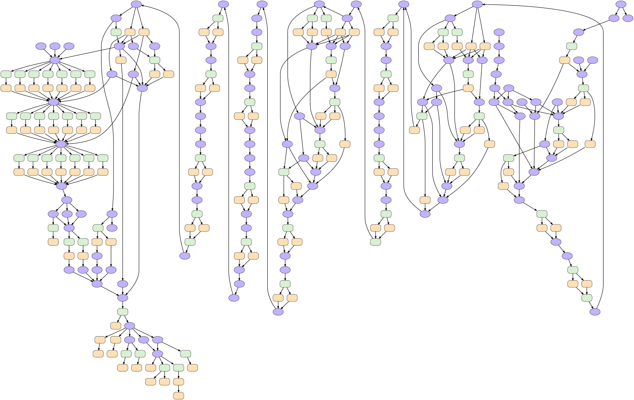
Figure 2Illustration of the computational complexity of the COSMO dynamical core, using a CDAG. The nodes of the graph represent computational kernels (blue ellipses) that can have multiple input and output variables, halo updates (green rectangles), and boundary condition operations (orange rectangles). The edges of the graph represent data dependencies. Since the dynamical core of COSMO has been written using a DSL, the CDAG can be produced automatically using an analysis back end of the DSL compiler. The lengthy serial section in the middle of the figure corresponds to the sound waves sub-stepping in the fast-wave solver. The parallel section in the upper left corresponds to the advection of the seven tracer variables. CDAGs can automatically be produced from C++ code.
For the simulations presented in this paper, we use a refactored version 5.0 of the regional weather and climate code developed by COSMO (COSMO, 2017; Doms and Schättler, 1999; Steppeler et al., 2002) and – for the climate mode – the Climate Limited-area Modelling (CLM) Community (CLM-Community, 2017). At kilometer-scale resolution, COSMO is used for numerical weather prediction (Richard et al., 2007; Baldauf et al., 2011) and has been thoroughly evaluated for climate simulations in Europe (Ban et al., 2015; Leutwyler et al., 2017). The COSMO model is based on the thermo-hydrodynamical equations describing non-hydrostatic, fully compressible flow in a moist atmosphere. It solves the fully compressible Euler equations using finite difference discretization in space (Doms and Schättler, 1999; Steppeler et al., 2002). For time stepping, it uses a split-explicit three-stage second-order Runge–Kutta discretization to integrate the prognostic variables forward in time (Wicker and Skamarock, 2002). For horizontal advection, a fifth-order upwind scheme is used for the dynamic variables and a Bott scheme (Bott, 1989) is used for the moisture variables. The model includes a full set of physical parametrizations required for real-case simulations. For this study, we use a single-moment bulk cloud microphysics scheme that uses five species (cloud water, cloud ice, rain, snow, and graupel) described in Reinhardt and Seifert (2006). For the full physics simulations, additionally a radiation scheme (Ritter and Geleyn, 1992), a soil model (Heise et al., 2006), and a sub-grid-scale turbulence scheme (Raschendorfer, 2001) are switched on.
The COSMO model is a regional model and physical space is discretized in a rotated latitude–longitude–height coordinate system and projected onto a regular, structured, three-dimensional grid (IJK). In the vertical, a terrain-following coordinate supports an arbitrary topography. The spatial discretization applied to solve the governing equations generates so called stencil computations (operations that require data from neighboring grid points). Due to the strong anisotropy of the atmosphere, implicit methods are employed in the vertical direction, as opposed to the explicit methods applied to the horizontal operators. The numerical discretization yields a large number of mixed compact horizontal stencils and vertical implicit solvers, strongly connected via the data dependencies on the prognostic variables. Figure 2 shows the data dependency graph of the computational kernels of the dynamical core of COSMO used in this setup, where each computational kernel corresponds to a complex set of fused stencil operations in order to maximize the data locality of the algorithm. Each computational kernel typically has multiple input and output fields and thus data dependencies as indicated with the edges of the Computational Directed Acyclic Graph (CDAG) shown in Fig. 2. Maximizing the data locality of these stencil computations is crucial to optimize the time to solution of the application.
To enable the running of COSMO on hybrid high-performance computing systems with GPU-accelerated compute nodes, we rewrote the dynamical core of the model, which implements the solution to the non-hydrostatic Euler equations, from Fortran to C++ (Fuhrer et al., 2014). This enabled us to introduce a new C++ template library-based domain-specific language (DSL) we call Stencil Loop Language (STELLA) (Gysi et al., 2015a) to provide a performance-portable implementation for the stencil algorithmic motifs by abstracting hardware-dependent optimization. Specialized back ends of the library produce efficient code for the target computing architecture. Additionally, the DSL supports an analysis back end that records the access patterns and data dependencies of the kernels shown in Fig. 2. This information is then used to determine the amount of memory accesses and to assess the memory utilization efficiency. For GPUs, the STELLA back end is written in CUDA, and other parts of the refactored COSMO implementation use OpenACC directives (Lapillonne and Fuhrer, 2014).
Thanks to this refactored implementation of the model and the STELLA DSL, COSMO is the first fully capable weather and climate model to go operational on GPU-accelerated supercomputers (Lapillonne et al., 2016). In the simulations we analyze here, the model was scaled to nearly 5000 GPU-accelerated nodes of the Piz Daint supercomputer at the Swiss National Supercomputing Centre.5 To our knowledge, COSMO is still the only production-level weather and climate model capable of running on GPU-accelerated hardware architectures.
3.2 Hardware description
The experiments were performed on the hybrid partition of the Piz Daint supercomputer, located at the Swiss National Supercomputing Centre (CSCS) in Lugano. At the time when our simulation was performed, this supercomputer consisted of a multi-core partition, which was not used in this study, as well as a hybrid partition of 4'936 Cray XC50 nodes. These hybrid nodes are equipped with an Intel E5-2690 v3 CPU (code name Haswell) and a PCIe version of the NVIDIA Tesla P100 GPU (code name Pascal) with 16 GBytes second-generation high-bandwidth memory (HBM2).6 The nodes of both partitions are interconnected in one fabric (based on Aries technology) in a Dragonfly topology (Alverson et al., 2012).
3.3 Energy measurements
We measure the energy to solution of our production-level runs on Piz Daint using the methodology established and described in detail by Fourestey et al. (2014). The resource utilization report provided on Cray systems for a job provides the total energy (En) consumed by each application run on N compute nodes. The total energy (which includes the interconnect) is then computed using
where τ is the wall time for the application, the W × τ term accounts for the 100 W per blade contribution from the Aries interconnect, and the 0.95 on the denominator adjusts for AC/DC conversion.
3.4 Simulation setup and verification
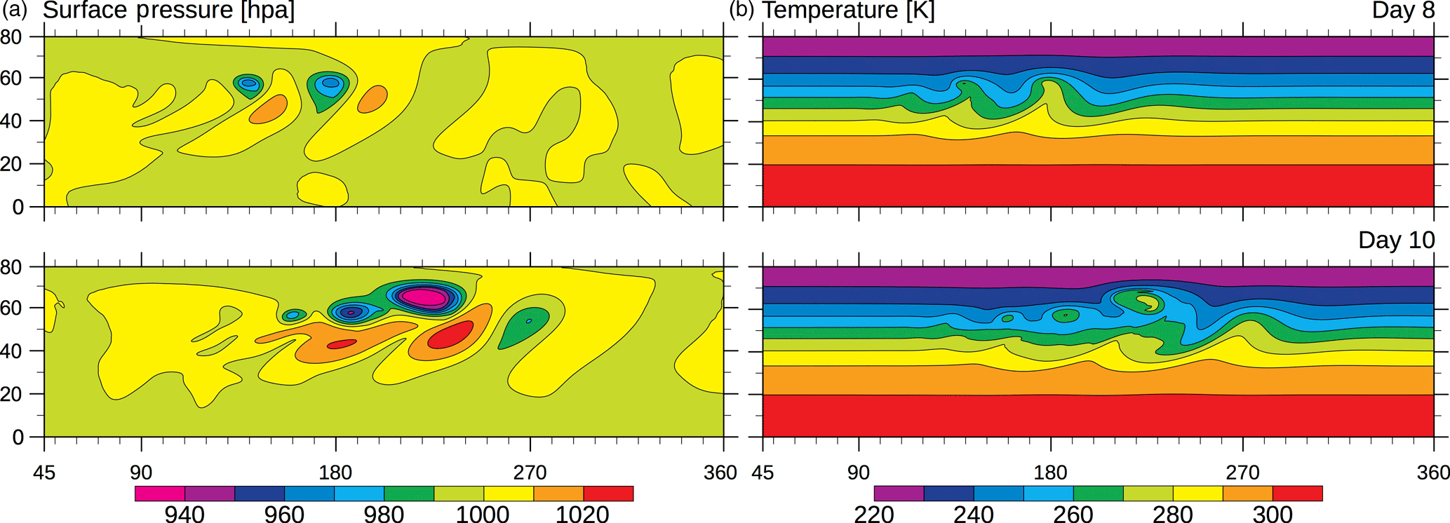
Figure 3Evolution of a baroclinic wave in a dry simulation with 47 km grid spacing on day 8 and 10: (a) surface pressure and (b) temperature on the 850 hPa pressure level (roughly 1.5 km above sea level).
When pushing ahead the development of global high-resolution climate models, there are two complementary pathways. First, one can refine the resolution of existing global climate models (Miura et al., 2007). Second, one may alternatively try to expand the computational domain of high-resolution limited-area models towards the global scale (Bretherton and Khairoutdinov, 2015). Here we choose the latter and develop a near-global model from the limited-area high-resolution model COSMO.
We perform near-global simulations for a computational domain that extends to a latitude band from 80∘ S to 80∘ N, which covers 98.4 % of the surface area of planet Earth. The simulation is inspired by the test case used by the winner of the 2016 Gordon Bell Prize (Yang et al., 2016a).
The simulations are based on an idealized baroclinic wave test (Jablonowski and Williamson, 2006), which can be considered a standard benchmark for dynamical cores of atmospheric models. The test describes the growth of initial disturbances in a dynamically unstable westerly jet stream into finite-amplitude low- and high-pressure systems. The development includes a rapid transition into a nonlinear regime, accompanied by the formation of sharp meteorological fronts, which in turn trigger the formation of complex cloud and precipitation systems.
The setup uses a two-dimensional (latitude–height) analytical description of a hydrostatically balanced atmospheric base state with westerly jet streams below the tropopause, in both hemispheres. A large-scale local Gaussian perturbation is then applied to this balanced initial state which triggers the formation of a growing baroclinic wave in the Northern Hemisphere, evolving over the course of several days (Fig. 3). To allow moist processes, the dry initial state is extended with a moisture profile (Park et al., 2013) and the parametrization of cloud-microphysical processes is activated.
The numerical problem is discretized on a latitude–longitude grid with up to 36 000 × 16 001 horizontal grid points for the 930 m simulation. In the zonal direction the domain is periodic and at 80∘ north/south confined by boundary conditions, relaxing the evolving solution against the initial conditions in a 500 km wide zone. The vertical direction is discretized using 60 stretched model levels, spanning from the surface to the model top at 40 km. The respective layer thickness widens from 20 m at the surface to 1.5 km near the domain top.
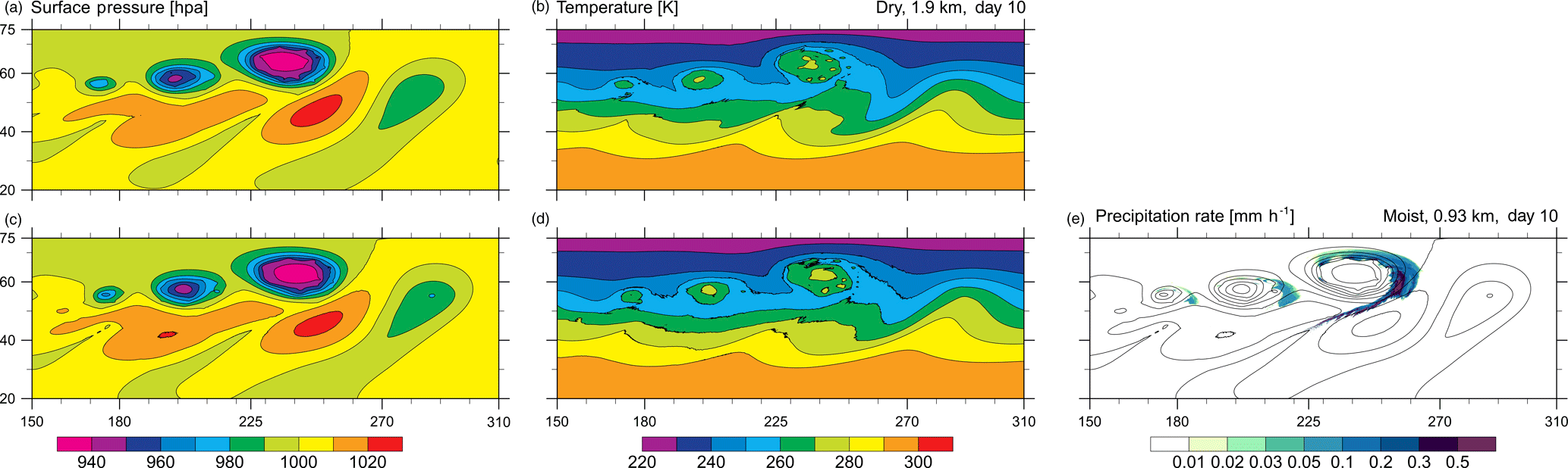
Figure 4Output of the baroclinic wave (day 10): (a, b) dry simulation with 1.9 km grid spacing, (c, d, e) moist simulation with 0.93 km grid spacing, (a, c) surface pressure, (b, d) temperature on the 850 hPa pressure level, and (e) precipitation.
For the verification against previous dry simulations, a simulation at 47 km grid spacing is used. The evolution of the baroclinic wave (Fig. 3) very closely follows the solution originally found by Jablonowski and Williamson (2006, see their Fig. 5). At day 8 of the simulation, three low-pressure systems with frontal systems have formed, and at day 10 wave breaking is evident. At this time, the surface temperature field shows cutoff warm-core cyclonic vortices.
The evolution in the moist and the dry simulation at very high resolution is shown in Fig. 4. The high-resolution simulations reveal the onset of a secondary (likely barotropic) instability along the front and the formation of small-scale warm-core vortices with a spacing of up to 200–300 km. The basic structure of these vortices is already present in the dry simulation, but they exhibit considerable intensification and precipitation in the moist case. The formation of a large series of secondary vortices is sometimes observed in maritime cases of cyclogenesis (Fu et al., 2004; Ralph, 1996) but appears to be a rather rare phenomena. However, it appears that cases with one or a few secondary vortices are not uncommon and they may even be associated with severe weather (Ludwig et al., 2015).
The resulting cloud pattern is dominated by the comma-shaped precipitating cloud that forms along the cold and occluded fronts of the parent system (Fig. 1). The precipitation pattern is associated with stratiform precipitation in the head of the cloud and small patches with precipitation rates exceeding 5 mm h−1 in their tail, stemming from small embedded convective cells. Looking closely at the precipitation field (Fig. 4e), it can be seen that the secondary vortices are colocated with small patches of enhanced precipitation.
In the past, the prevalent metric to measure the performance of an application was the number of floating point operations executed per second (flop s−1). It used to pay off to minimize the number of required floating point operations in an algorithm and to implement the computing system in such a way that a code would execute many such operations per second. Thus, it made sense to assess application performance with the flop s−1 metric. However, the world of supercomputing has changed. Floating point operations are now relatively cheap. They cost about a factor of 1000 less if measured in terms of energy needed to move operands between memory and registers, and they execute several hundred times faster compared to the latency of memory operations. Thus, algorithmic optimization today has to focus on minimizing data movement, and it may even pay off to recompute certain quantities if this avoids data movements. In fact, a significant part of the improvements in time to solution in the refactored COSMO code are due to the recomputation of variables that were previously stored in memory – the original code was written for vector supercomputers in the 1990s. On today's architectures, it may even pay off to replace a floating point minimal sparse algorithm with a block-sparse algorithm, into which many trivial zero operations have been introduced (Hutter et al., 2014). Using the flop s−1 metric to characterize application performance could be very misleading in these cases.
A popular method to find performance bottlenecks of both compute- and memory-bound applications is the roofline model (Williams et al., 2009). However, assessing performance of an application simply in terms of sustained memory bandwidth, which is measured in bytes per second, would be equally deceptive. For example, by storing many variables in memory, the original implementation of COSMO introduces an abundance of memory movements that boost the sustained memory bandwidth but are inefficient on modern processor architectures, since these movements cost much more than the recomputation of these variables.
Furthermore, full-bandwidth utilization on modern accelerator architectures, such as the GPUs used here, requires very specific conditions. Optimizing for bandwidth utilization can lead the application developer down the wrong path because unaligned, strided, or random accesses can be intrinsic to an underlying algorithm and severely impact the bandwidth (Lee et al., 2010). Optimizations to improve alignment or reduce the randomness of memory accesses may introduce unnecessary memory operations that could be detrimental to time to solution or energy efficiency.
Thus, in order to properly assess the quality of our optimizations, one needs to directly consider data movement. Here we propose a method how this can be done in practice for the COSMO dynamical core and present the resulting MUE metric.
Our proposal is motivated by the full-scale COSMO runs we perform here, where 74 % of the total time is spent in local stencil computations. The dependencies between stencils in complex stencil programs can be optimized with various inlining and unrolling techniques (Gysi et al., 2015a). Thus, to be efficient, one needs to achieve maximum spatial and temporal data reuse to minimize the number of data movement operations and perform them at the highest bandwidth.
In order to assess the efficiency in memory usage of an implementation on a particular machine, one needs to compare the actual number of data transfers executed,7 which we denote with D, with the necessary data transfers Q of the algorithm. Q is the theoretical lower bound (Hong and Kung, 1981) of the number of memory accesses required to implement the numerical algorithm.
The MUE can be intuitively interpreted as how well the code is optimized both for data locality and bandwidth utilization; i.e., if MUE = 1, the implementation reaches the memory movement lower bound of the algorithm and performs all memory transfers with maximum bandwidth. Formally,
where B and represent the bandwidth achieved by an implementation and maximum achievable bandwidth, respectively.
In order to compute the MUE for COSMO, we developed a performance model that combines the theoretical model from Hong and Kung (1981), hypergraph properties, and graph partitioning techniques to estimate the necessary data transfer, Q, from the CDAG information of COSMO. By partitioning the CDAG into subcomputations that satisfy certain conditions imposed by the architecture, this model determines the theoretical minimum amount of memory transfers by maximizing the data locality inside the partitions. To approximate the number of actual transfers D, we use the same technique to evaluate the quality of current COSMO partitioning. The values B and were measured empirically – the former by profiling our application and the latter by a set of micro-benchmarks.
The details of how to determine the MUE for COSMO are given in Appendix A. The MUE metric cannot be used to compare different algorithms but is a measure of the efficiency of an implementation of a particular algorithm on a particular machine, i.e., how much data locality is preserved and what the achieved bandwidth is. It thus complements other metrics such as SYPD and may complement popular metrics such as flop s−1 or memory bandwidth. As compared to the frequently applied roofline model, the MUE metric also includes the schedule of operations, not simply the efficient use of the memory subsystem. It is thus a stronger but also more complex metric.
To establish a performance baseline for global kilometer-scale simulations, we here present a summary of the key performance metrics for the simulations at 930 m, 1.9 km, and 47 km grid spacing, as well as a study of weak and strong scalability.
5.1 Weak scalability
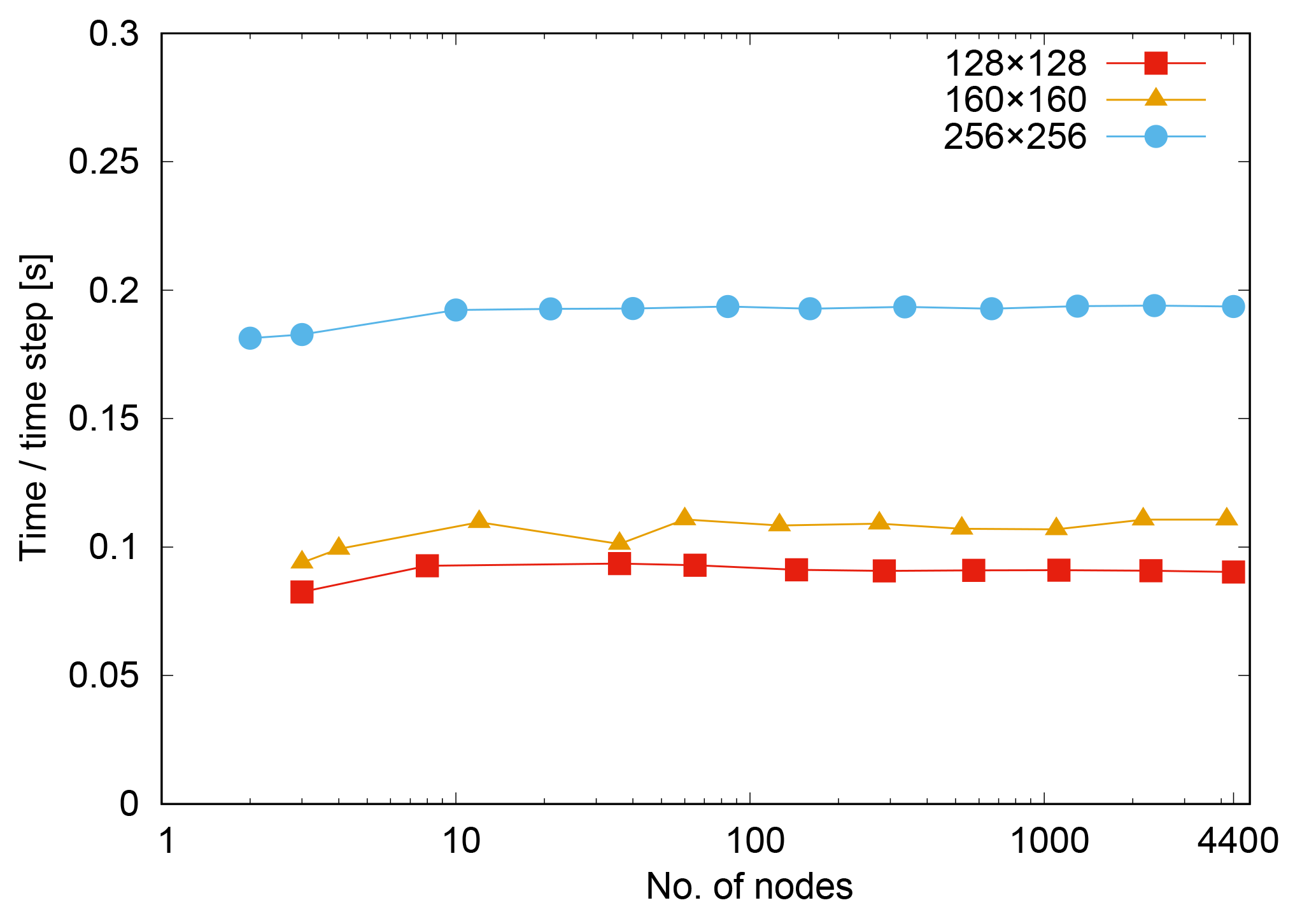
Figure 5Weak scalability on the hybrid P100 Piz Daint nodes, per COSMO time step of the dry simulation.
Until this study the GPU version of COSMO had only been scaled up to 1000 nodes of the Piz Daint supercomputer (Fuhrer et al., 2014), while the full machine – at the time of the experiment – provides 4932 nodes. The scaling experiments (weak and strong) were performed with the dry simulation setup. Including a cloud microphysics parametrization, as used in the moist simulation (Fig. 4), increases time to solution by about 10 %. Since microphysics does not contain any inter-node communication and is purely local to a single column of grid points, we do not expect an adverse impact on either weak or strong scalability.
Figure 5 shows weak scaling for three per-node domain sizes ranging from 128×128 to 256×256 grid points in the horizontal, while keeping the size in the vertical direction fixed at 60 grid points. In comparison, on 4888 nodes, the high-resolution simulations at 930 m and 1.9 km horizontal grid spacing correspond to a domain size per node of about 346×340 and 173×170.8 The model shows excellent weak scalability properties up to the full machine, which can at least partially be explained by the nearest-neighbor halo-exchange pattern. This property reduces the complexity of COSMO's scalability on Piz Daint to the strong scaling behavior of the code. Essentially, the number of grid points per node determines the achievable time to solution of a given problem.
5.2 Strong scalability

Figure 6Strong scalability on Piz Daint: on P100 GPUs (filled symbols) and on Haswell CPUs using 12 MPI ranks per node (empty symbols).
From earlier scaling experiments of the STELLA library (Gysi et al., 2015b) and the GPU version of COSMO (Fuhrer et al., 2014; Leutwyler et al., 2016), it is known that, for experiments in double precision on Tesla K20x, linear scaling is achieved as long as the number of grid points per node exceeds about 64×64 to 128×128 grid points per horizontal plane. In comparison, single-precision measurements on Tesla P100 already start to saturate at a horizontal domain size of about 200×200 grid points per node (Fig. 6),9 corresponding to about 32 nodes for a 19 km setup and about 1000 nodes for a 3.7 km setup. Since with the 930 m and 1.9 km setup we are already in 930 m or close to 1.9 km, the linear scaling regime on the full machine, we here chose a coarser horizontal grid spacing of 3.7 and 19 km. The lower limit on the number of nodes is given by the GPU memory of 16 GB. In addition to the GPU benchmarks (filled symbols), we measured the performance with the CPU version of COSMO (empty symbols), using 12 MPI (Message Passing Interface) ranks per CPU, i.e., one MPI rank per Haswell core.10 Exceeding 1000 nodes (38×38 grid points per node) execution on CPUs yields a shorter time to solution than on GPUs.
5.3 Time to solution
Table 1Time compression (SYPD) and energy cost (MWh SY−1) for three moist simulations: at 930 m grid spacing obtained with a full 10-day simulation, at 1.9 km from 1000 steps, and at 47 km from 100 steps.
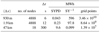
On 4888 nodes, a 10-day long moist simulation at 930 m grid spacing required a wall time of 15.3 h at a rate of 0.043 SYPD (Table 1), including a disk I/O load of five 3-D fields and seven 2-D fields,11 written periodically every 12 h of the simulation. Short benchmark simulations at 1.9 and 47 km, integrated for 1000 and 100 time steps, respectively, yield 0.23 and 9.6 SYPD. As mentioned earlier, the minimum value required for AMIP-type simulations is 0.2–0.3 SYPD. While for the 47 km setup scalability already starts to saturate, even with the 18 nodes reported (Table 1), the high-resolution simulations, with an approximate per-node domain size of and , are still in a regime of good scalability. We have also conducted a 1.9 km simulation with a full set of physical parametrizations switched on, and this increases the time to solution by 27 % relative to the moist simulations presented here.
In conclusion, the results show that AMIP-type simulations at horizontal grid spacings of 1.9 km using a fully fledged atmospheric model are already feasible on Europe's highest-ranking supercomputer. In order to reach resolutions of 1 km, a further reduction of time to solution of at least a factor of 5 is required.
In the remainder of this section, we attempt a comparison of our results at 1.9 km against the performance achieved by Yang et al. (2016a) in their 2 km simulation (as their information for some of the other simulations is incomplete). They argue that for an implicit solver the time step can be kept at 240 s independent of the grid spacing and report (see their Figs. 7 and 9) values of 0.57 SYPD for a grid spacing of 2 km, on the full TaihuLight system. As explained in Sect. 2, such large time steps are not feasible for global climate simulations resolving convective clouds (even when using implicit solvers), and a maximum time step of 40–80 s would very likely be needed; this would decrease their SYPD by a factor of 3 to 6. Furthermore, their simulation covers only 32 % of the Earth's surface (18∘ N to 72∘) but uses twice as many levels; this would further reduce their SYPD by a factor of 1.5. Thus we estimate that the simulation of Yang et al. (2016a) at 2 km would yield 0.124 to 0.064 SYPD when accounting for these differences. In comparison, our simulation at 1.9 km yields 0.23 SYPD; i.e., it is faster by at least a factor of 2.5. Note that this estimate does not account for additional simplifications in their study (neglect of microphysical processes, spherical shape of the planet, and topography). In summary, while a direct comparison with their results is difficult, we argue that our results can be used to set a realistic baseline for production-level GCM performance results and represent an improvement by at least a factor of 2 with respect to previous results.
5.4 Energy to solution
Based on the power measurement (see Sect. 3.3) we now provide the energy cost of full-scale simulations (Table 1) using the energy cost unit MWh per simulation year (MWh/SY). The 10-day long simulation at 930 m grid spacing running on 4888 nodes requires 596 MWh SY−1, while the cost of the simulation at 1.9 km on 4888 nodes is 97.8 MWh SY−1. For comparison, the coarse resolution at 47 km simulation on a reduced number of nodes (18) requires only 0.01 MWh SY−1.
A 30-year AMIP-type simulation (with full physics) at a horizontal grid spacing of 1 km on the Piz Daint system would take 900 days to complete, resulting in an energy cost of approximately 22 GWh – which approximately corresponds to the consumption of 6500 households during 1 year.
Again, we attempt a comparison with the simulations performed by Yang et al. (2016a). The Piz Daint system reports a peak power draw of 2052 kW when running the high-performance LINPACK (HPL) benchmark. The sustained power draw when running the 930 m simulation amounted to 1059.7 kW, thus 52 % of the HPL value. The TaihuLight system reports a sustained power draw for the HPL benchmark of 15 371 kW (TOP500, 2017). While Yang et al. (2016a) do not report power consumption of their simulations, we expect the simulations on Piz Daint to be at least 5 times more power efficient, even when assuming similar achieved SYPD (see above).12
5.5 Simulation efficiency
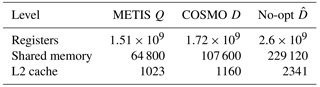
Table 2Data transfer cost estimations of the dynamical core for a theoretical lower bound (METIS), dynamical core implementation using the STELLA library (COSMO), and non-optimized dynamical core implementation (no-merging).
In view of the energy consumption, it is paramount to consider the efficiency of the simulations executed. We do this here by considering the memory usage efficiency metric introduced in Sect. 4.
To estimate a solution for the optimization problem described in Appendix A, Eq. (A2), we use the METIS library (Karypis and Kumar, 2009). The results are presented in Table 2. The METIS Q column is the approximation of the lower bound Q obtained from the performance model using the METIS library. The COSMO D column is the evaluation of current COSMO partitioning in our model. The no-opt column shows the amount of data transfers of COSMO if no data locality optimization techniques are applied, like in the original Fortran version of the code. Since the original CDAG is too large for the minimization problem of the performance model, three different simplified versions of the CDAG, which focus on the accesses to three different layers of the memory hierarchy of the GPU, are studied: registers, shared memory, and L2 cache.
The model shows how efficient COSMO is in terms of data transfers – it generates only 14, 66, and 13 % more data transfers than the lower bound in the register, shared memory, and L2 cache layers, respectively. The sophisticated data locality optimization techniques of the STELLA implementation of the dynamical core of COSMO result in very good data reuse. On the P100, all memory accesses to/from DRAM go through the L2 unit. Therefore, we focus on the efficiency of this unit such that
where DL2 and QL2 stand for estimated number of main memory operations and its lower bound, respectively.
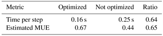
Table 3Performance model verification results. Measured dynamical core time step execution time for the STELLA implementation optimized for data locality and the non-optimized implementation compared against the corresponding MUE metric.
The model also can estimate the efficiency of our optimizations. Assuming that we can reach the peak achievable bandwidth if we perform no data locality optimizations (), then
It can be seen that
This result shows the importance of data locality optimizations – the optimized implementation is more than 50 % faster than a potential version that achieves peak bandwidth while using no data locality techniques.
To validate the model results, we have conducted single-node runs with and without data locality optimizations. Bandwidth measurements of the non-optimized version are very close to maximum achievable bandwidth (not shown). The fact that the two ratios in the third column of Table 3 agree is testimony to the high precision of the performance model.
The work presented here sets a new baseline for fully fledged kilometer-scale climate simulations on a global scale. Our implementation of the COSMO model that is used for production-level numerical weather predictions at MeteoSwiss has been scaled to the full system on 4888 nodes of Piz Daint, a GPU-accelerated Cray XC50 supercomputer at the Swiss National Supercomputing Centre (CSCS). The dynamical core has been fully rewritten in C++ using a DSL that abstracts the hardware architecture for the stencil algorithmic motifs and enables sophisticated tuning of data movements. Optimized back ends are available for multi-core processors with OpenMP, GPU accelerators with CUDA, and for performance analysis.
The code shows excellent strong scaling up to the full machine size when running at a grid spacing of 4 km and below, on both the P100 GPU accelerators and the Haswell CPU. For smaller problems, e.g., at a coarser grid spacing of 47 km, the GPUs run out of parallelism and strong scalability is limited to about 100 nodes, while the same problem continues to scale on multi-core processors to 1000 nodes. Weak scalability is optimal for the full size of the machine. Overall, performance is significantly better on GPUs as compared to CPUs for the high-resolution simulations.
The simulations performed here are based on the idealized baroclinic wave test (Jablonowski and Williamson, 2006), which is part of the standard procedure to test global atmospheric models. Our results are validated against the original solution published in this paper.
We measured time to solution in terms of simulated years per wall clock day (SYPD) for a near-global simulation on a latitude band from 80∘ S to 80∘ N that covers 98.4 % of planet Earth's surface. Running on 4888 P100 GPUs of Piz Daint, currently Europe's largest supercomputer, we measured 0.23 SYPD at a 1.9 km grid spacing. This performance is adequate for numerical weather predictions and 10-year scale climate studies. Simulations at this resolution had an energy cost of 97.8 MWh SY−1.
In a moist simulation with 930 m horizontal grid spacing, we observed the formation of frontal precipitating systems, containing embedded explicitly resolved convective motions, and additional cutoff warm-core cyclonic vortices. The explicit representation of embedded moist convection and the representation of the resolved instabilities exhibits physically different behavior from coarser-resolution simulations. This is testimony to the usefulness of the high-resolution approach, as a much expanded range of scales and processes is simulated. Indeed it appears that for the current test case, the small vortices have not previously been noted, as the test case appears to converge for resolutions down to 25 km (Ullrich et al., 2015), but they clearly emerge at kilometer-scale resolution.
These results serve as a baseline benchmark for global climate model applications. For the 930 m experiment we achieved 0.043 SYPD on 4888 GPU-accelerated nodes, which is approximately one-seventh of the 0.2–0.3 SYPD required to conduct AMIP-type simulations. The energy cost for simulations at this horizontal grid spacing was 596 MWh SY−1.
Scalable global models do not use a regularly structured grid such as COSMO, due to the “pole problem”. Therefore, scalable global models tend to use quasi-uniform grids such as cubed-sphere or icosahedral grids. We believe that our results apply directly to global weather and climate models employing structured grids and explicit, split-explicit, or horizontally explicit, vertically implicit (HEVI) time discretizations (e.g., FV3, NICAM). Global models employing implicit or spectral solvers may have a different scaling behavior.
Our work was inspired by the dynamical core solver that won the 2016 Gordon Bell award at the Supercomputing Conference (Yang et al., 2016a). The goal of this award is to reward high performance achieved in the context of a realistic computation. A direct comparison with the results reported there is difficult, since Yang et al. (2016a) were running a research version of a dynamical core solver and COSMO is a fully fledged regional weather and climate model. Nevertheless, our analysis indicates that our benchmarks represent an improvement both in terms of time to solution and energy to solution. As far as we know, our results represent the fastest (in terms of application throughput measured in SYPD at 1 km grid spacing) simulation of a production-ready, non-hydrostatic climate model on a near-global computational domain.
In order to reach the 3–5 SYPD performance necessary for long climate runs, simulations would be needed that run 100 times faster than the baseline we set here. Given that Piz Daint with NVIDIA P100 GPUs is a multi-petaflop system, the 1 km scale climate runs at 3–5 SYPD performance represent a formidable challenge for exascale systems. As such simulations are of interest to scientists around the globe, we propose that this challenge be defined as a goal post to be reached by the exascale systems that will be deployed in the next decade.
Finally, we propose a new approach to measure the efficiency of memory bound application codes, like many weather and climate models, running on modern supercomputing systems. Since data movement is the expensive commodity on modern processors, we advocate that the code's performance on a given machine be characterized in terms of data movement efficiency. We note that both detailed mathematical analysis and the general applicability of our MUE metric is beyond the scope of this paper and requires additional publication. In this work we show a use case of the MUE metric and demonstrate its precision and usefulness in assessing memory subsystem utilization of a machine, using the I/O complexity lower bound as the necessary data transfers, Q, of the algorithm. With the time to solution and the maximum system bandwidth , it is possible to determine the memory usage efficiency that captures how well the code is optimized both for data locality and bandwidth utilization. It will be interesting to investigate the MUE metric in future performance evaluations for weather and climate codes on high-performance computing systems.
The particular version of the COSMO model used in this study is based on the official version 5.0 with many additions to enable GPU capability and available under license (http://www.cosmo-model.org/content/consortium/licencing.htm for more information). These developments are currently in the process of being reintegrated into the mainline COSMO version. COSMO may be used for operational and for research applications by the members of the COSMO consortium. Moreover, within a license agreement, the COSMO model may be used for operational and research applications by other national (hydro-)meteorological services, universities, and research institutes. The model output data will be archived for a limited amount of time and are available on request.
Here, we discuss how to determine the memory usage efficiency (MUE) given in Eq. (2) for an application code, such as the COSMO model. We need to determine the necessary data transfers Q, the maximum system bandwidth , and measure the execution time T.
Necessary transfers Q
A natural representation of data flow and dependencies of algorithms is a CDAG. This abstraction is widely used for register allocation optimization, scheduling problems, and communication minimization. A CDAG models computations as vertices (V) and communications as edges (E) between them. A CDAG can be used to develop theoretical models that reason about data movements of an application. However, not all the edges of the CDAG account for data transfers, since the data required by a computation might be stored in fast memory (cached), depending on the execution schedule. Finding an execution schedule that minimizes the transaction metric is NP-hard for general CDAGs and therefore an intractable problem (Kwok and Ahmad, 1999).
Minimizing data movement has been the subject of many studies. Two main approaches have been established: (1) finding analytical lower bounds for chosen algorithms for a given machine model (Hong and Kung, 1981; Vetter, 2001; Goodrich et al., 2010) and (2) finding optimal graph partitions (Gadde, 2013). The former is designed for particular, highly regular small algorithms, like sorting (Vetter, 2001) or matrix multiplication (Hong and Kung, 1981) and is not suitable for large-scale applications like COSMO. The latter approach is mostly used for minimizing network communication (Liu et al., 2014) and has not been applied to large applications either. In our performance model, we combine the two into a novel graph-cutting technique. We build on Hong and Kung's 2S partitioning (Hong and Kung, 1981) and construct a hypergraph partitioning technique to estimate a memory movement lower bound. We do not consider internode communication here. To the best of our knowledge, we are the first to apply these techniques to a real-world parallel application.
The key concept behind estimating Q is to partition the whole CDAG into subcomputations (2S partitions) , such that each Pi requires at most S data transfer operations. Then, if H(2S) is the minimal number of 2S partitions for a given CDAG, Hong and Kung (1981) showed that the minimal number Q of memory movement operations for any valid execution of the CDAG is bounded by
Here we outline the key steps of our modeling approach:
-
We reduce Hong and Kung's 2S partitioning (Hong and Kung, 1981) definition to hypergraph cut by relaxing the constraints on the dominator and minimum set sizes. Each hyper-edge contains a vertex from the original CDAG and all its successors.
-
We approximate the minimal hypergraph cut by minimizing the total communication volume.
-
We then express the memory movement lower bound as
subject to
where Nbr(v) is the number of partitions that vertex v is adjacent to, w(v) is the memory size of vertex v, and S is the size of memory at a level for which the optimization is performed. Equation (A2) now minimizes the sum of the communication volume across all partitions (assuming we load partitions one after the other), while constraint Eq. (A5) bounds the boundary weight for each partition to 2S such that it fits in fast memory.
A2 COSMO CDAG
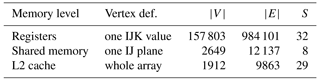
Figure 2 shows the data dependency CDAG of the computational kernels of the dynamical core of COSMO, where each kernel corresponds to a complex set of fused stencil operations in order to maximize the data locality of the algorithm. A single time step in COSMO accesses 781 variables, each of which is represented by a array for our 930 m simulation. Some variables are updated multiple times during a time step which results in a total number of variable accesses (CDAG vertices) of more than 1010. The resulting large and complex graph makes estimating Q impractical. In order to reduce the complexity, one can coarsen the CDAG by grouping multiple accesses into a single vertex. As an example, Fig. 2 shows the coarsest representation of the CDAG where each vertex models a full kernel. Each kernel may read and write various output variables, compute multiple stencil operations and boundary conditions, or perform halo exchanges. Thus, in this coarsened version, valuable data dependency information is lost, and one cannot argue about the optimality and possible rearrangement of the operations fused within a kernel.
We now describe how we determine coarsening strategies of the COSMO CDAG for three levels of the memory hierarchy of our target system, registers, shared memory, and L2 cache.
-
Registers (65'536): the COSMO GPU implementation assigns all computations accessing variables with the same IJ coordinate to the same GPU thread and use registers to reuse values in the K direction. To model this memory hierarchy, it is only necessary to keep the stencil accesses in the K direction. Thus, all accesses in the IJ plane are represented as a single vertex in the CDAG, which is then simplified to 781 variables and their dependencies among all 60 levels in K.
-
Shared memory (64 kB): the shared memory of the GPU is used to communicate values between the different compute threads. In order to model this layer, all different accesses in the K direction of a variable are represented as a single vertex in the CDAG, while all accesses in the IJ plane are kept.
-
L2 cache (4 MB): this last cache level before DRAM is used to store whole arrays (fields). In this layer all accesses to a variable in any direction are represented as a vertex in the CDAG. It keeps only the data dependencies among variables, irrespective of the offset and direction of the access.
Table A1 lists details about the CDAGs at each of our three levels. Memory capacity of the GPU for each of the three layers is then used as a constraint to derive the parameter S (see values in Table A1). Values of the estimation of Q, obtained from the performance model for the three memory levels are shown in Table 2.
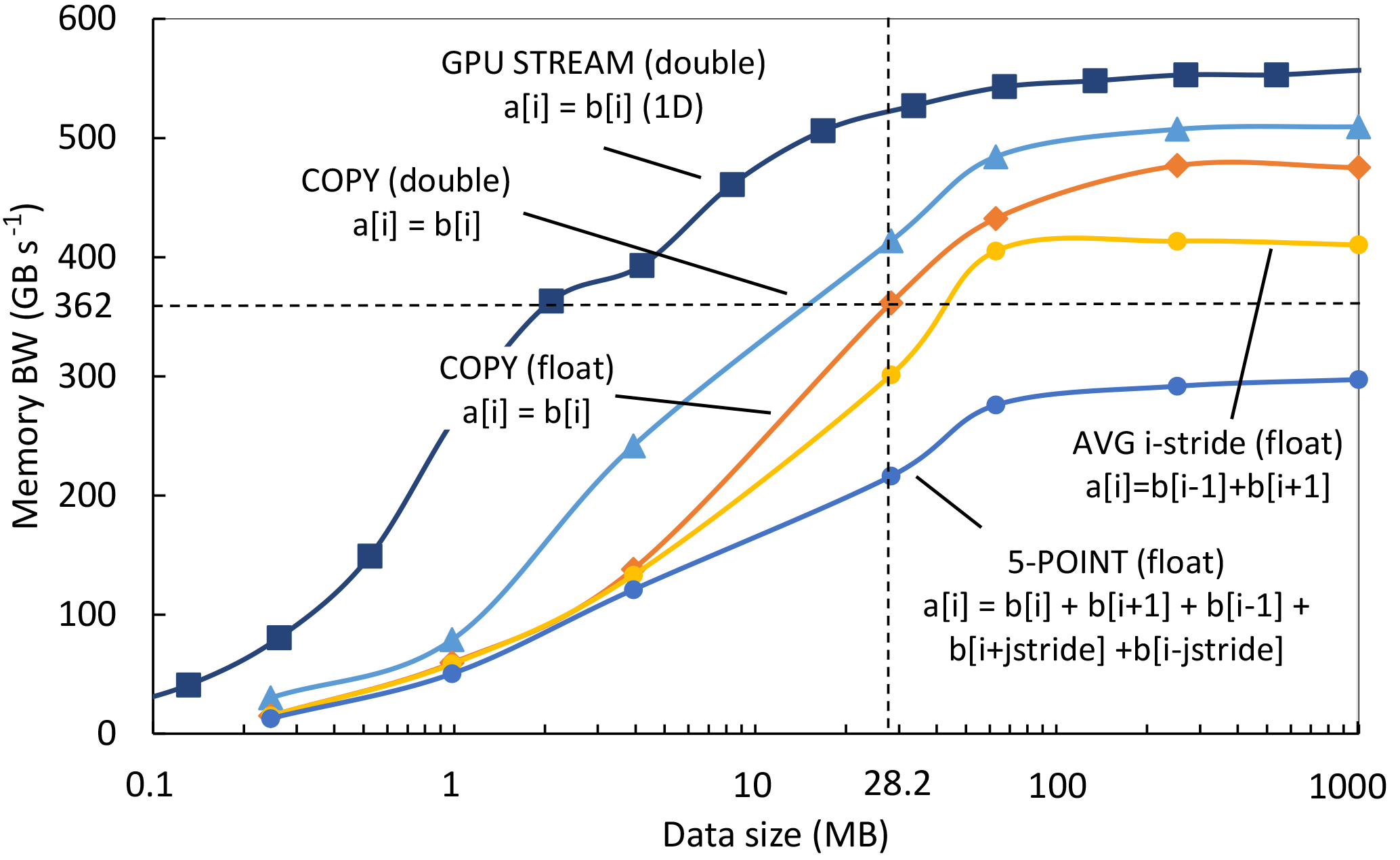
Figure A1Bandwidth of the representative stencil benchmarks and GPU STREAM on Tesla P100. All kernels (except for GPU STREAM) operate on a 3-D domain.
To generate the whole CDAG, we used the STELLA analysis back end (Gysi et al., 2015b) to trace all local memory accesses to all fields. Based on the information from the access offsets and order of operations, we reconstruct the read–write, write–read, and write–write dependencies.
Maximum achievable bandwidth
We now describe how we measure the memory usage efficiency in practice. We start by describing how to determine the maximum achievable bandwidth for COSMO stencils. Even though the Tesla P100 has a theoretical peak memory bandwidth of 720 GB s−1 (NVIDIA, 2016), we argue that this may not be achievable for real applications. A well-established method to measure the maximum achievable bandwidth of GPUs is the GPU STREAM benchmark (Deakin et al., 2016). Our tests show that the maximum achievable bandwidth for COPY is 557 GB s−1 if at least 30 MB double-precision numbers are copied (Fig. A1). However, stencil codes on multidimensional domains like COSMO require more complex memory access patterns that, even when highly tuned, cannot achieve the same bandwidth as STREAM due to architectural limitations.
We identified the most common patterns and designed and tuned a set of micro-benchmarks that only mimic the memory access patterns without the computations to investigate the machine capability of handling memory accesses for stencils. They include aligned, unaligned, and strided patterns in all dimensions. All benchmarks operate on a 3-D domain of parametric size, on either single- or double-precision numbers. The results of a representative set of four chosen micro-benchmarks are shown in Fig. A1, together with the GPU STREAM, which operates on 1-D domain. The fastest stencil kernel (double-precision aligned COPY) reaches 510 GB s−1. The slowdown compared to GPU STREAM is due to the more complex access pattern in the 3-D domain. Furthermore, using single-precision numbers further deteriorates the bandwidth on P100 (COPY (float) reaches 475 GB s−1). Our COSMO 930 m run uses predominantly single-precision numbers on a domain, which results in 28.2 MB of data per field. Our measurements show that the maximum achievable bandwidth for this setup is 362 GB s−1 (in the best case of the simple COPY benchmark). We will use this upper-bound number as the maximum system bandwidth. The average measured memory bandwidth across all COSMO real-world stencils is 276 GB s−1, which gives .
The authors declare that they have no conflict of interest.
This work was supported by the Swiss National Science Foundation under Sinergia grant
CRSII2_154486/1 and by a grant from the Swiss National Supercomputing Centre and PRACE.
We would like to acknowledge the many contributors to the GPU-capable version of COSMO
used in this study, among others Andrea Arteaga, Mauro Bianco, Isabelle Bey,
Christophe Charpilloz, Valentin Clement, Ben Cumming, Tiziano Diamanti, Tobias Gysi,
Peter Messmer, Katherine Osterried, Anne Roches, Stefan Rüdisühli, and Pascal Spörri.
Also, the authors would like to acknowledge the Center for Climate Systems Modeling
(C2SM) and the Federal Office of Meteorology and Climatology MeteoSwiss for their support.
Furthermore, we would like to thank Nils Wedi and Piotr Smolarkiewicz (ECMWF) for useful
comments and discussions. Finally, we would like to thank an anonymous reviewer,
Rupert W. Ford (STFC), and the topical editor of GMD (Sophie Valcke) for their constructive
comments and reviews that significantly improved the clarity and quality of the manuscript.
Edited by: Sophie Valcke
Reviewed by: Rupert W. Ford and one anonymous referee
Alverson, B., Froese, E., Kaplan, L., and Roweth, D.: Cray XC Series Network, Tech. Rep., available at: https://www.cray.com/sites/default/files/resources/CrayXCNetwork.pdf (last access: 3 April 2017), 2012. a
Balaji, V., Maisonnave, E., Zadeh, N., Lawrence, B. N., Biercamp, J., Fladrich, U., Aloisio, G., Benson, R., Caubel, A., Durachta, J., Foujols, M.-A., Lister, G., Mocavero, S., Underwood, S., and Wright, G.: CPMIP: measurements of real computational performance of Earth system models in CMIP6, Geosci. Model Dev., 10, 19–34, https://doi.org/10.5194/gmd-10-19-2017, 2017. a
Baldauf, M., Seifert, A., Foerstner, J., Majewski, D., Raschendorfer, M., and Reinhardt, T.: Operational Convective-Scale Numerical Weather Prediction with the COSMO Model: Description and Sensitivities, Mon. Weather Rev., 139, 3887–3905, 2011. a
Ban, N., Schmidli, J., and Schär, C.: Heavy precipitation in a changing climate: Does short-term summer precipitation increase faster?, Geophys. Res. Lett., 42, 1165–1172, 2015. a, b
Benoit, R., Schär, C., Binder, P., Chamberland, S., Davies, H. C., Desgagné, M., Girard, C., Keil, C., Kouwen, N., Lüthi, D., Maric, D., Müller, E., Pellerin, P., Schmidli, J., Schubiger, F., Schwierz, C., Sprenger, M., Walser, A., Willemse, S., Yu, W., and Zala, E.: The Real-Time Ultrafinescale Forecast Support during the Special Observing Period of the MAP, B. Am. Meteorol. Soc., 83, 85–109, 2002. a
Bony, S., Stevens, B., Frierson, D. M. W., Jakob, C., Kageyama, M., Pincus, R., Shepherd, T. G., Sherwood, S. C., Siebesma, A. P., Sobel, A. H., Watanabe, M., and Webb, M. J.: Clouds, circulation and climate sensitivity, Nat. Geosci., 8, 261–268, 2015. a
Borkar, S. and Chien, A. A.: The Future of Microprocessors, Commun. ACM, 54, 67–77, 2011. a
Bott, A.: A positive definite advection scheme obtained by nonlinear renormalization of the advective fluxes, Mon. Weather Rev., 117, 1006–1016, 1989. a
Boucher, O., Randall, D., Artaxo, P., Bretherton, C., Feingold, G., Forster, P., Kerminen, V.-M., Kondo, Y., Liao, H., Lohmann, U., Rasch, P., Satheesh, S. K., Sherwood, S., Stevens, B., and Zhang, X. Y.: Clouds and Aerosols. In: Climate Change 2013: The Physical Science Basis. Contribution of Working Group I to the Fifth Assessment Report of the Intergovernmental Panel on Climate Change, edited by: Stocker, T. F., Qin, D., Plattner, G.-K., Tignor, M., Allen, S. K., Boschung, J., Nauels, A., Xia, Y., Bex, V., and Midgley, P. M., Cambridge University Press, Cambridge, United Kingdom and New York, NY, USA, 571–658, https://doi.org/10.1017/CBO9781107415324.016, 2013. a
Bretherton, C. S. and Khairoutdinov, M. F.: Convective self-aggregation feedbacks in near-global cloud-resolving simulations of an aquaplanet, J. Adv. Model. Earth Syst., 7, 1765–1787, 2015. a, b
CLM-Community: Climate Limited-area Modelling Community, available at: http://www.clm-community.eu/, last access: 3 April, 2017. a
COSMO: Consortium for Small-Scale Modeling, available at: http://www.cosmo-model.org/, last access: 4 April, 2017. a
Davies, T., Staniforth, A., Wood, N., and Thuburn, J.: Validity of anelastic and other equation sets as inferred from normal-mode analysis, Q. J. Roy. Meteorol. Soc., 129, 2761–2775, 2003. a
Davies, T., Cullen, M. J., Malcolm, A. J., Mawson, M. H., Staniforth, A., White, A. A., and Wood, N.: A new dynamical core for the Met Office's global and regional modelling of the atmosphere, Q. J. Roy. Meteorol. Soc., 131, 1759–1782, https://doi.org/10.1256/qj.04.101, 2005. a
Deakin, T., Price, J., Martineau, M., and McIntosh-Smith, S.: GPU-STREAM v2.0: Benchmarking the Achievable Memory Bandwidth of Many-Core Processors Across Diverse Parallel Programming Models, 489–507, Springer, Cham, 2016. a
Doms, G. and Schättler, U.: The nonhydrostatic limited-area model LM (Lokal-Modell) of the DWD. Part I: Scientific documentation, Tech. rep., German Weather Service (DWD), Offenbach, Germany, available at: http://www.cosmo-model.org/ (last access: 19 March 2018), 1999. a, b
Durran, D. R.: Numerical Methods for Fluid Dynamics with Applications to Geophysics, Vol. 32 of Texts in Applied Mathematics, Springer, New York, 2010. a
ECMWF: IFS Documentation Part III: Dynamics and numerical procedures, European Centre for Medium-Range Weather Forecasts, Shinfield Park, Reading, RG2 9AX, England, 2016. a
Ewing, R. E. and Wang, H.: A summary of numerical methods for time-dependent advection-dominated partial differential equations, J. Comput. Appl. Math., 128, 423–445, numerical Analysis 2000, Vol. VII: Partial Differential Equations, 2001. a
Eyring, V., Bony, S., Meehl, G. A., Senior, C. A., Stevens, B., Stouffer, R. J., and Taylor, K. E.: Overview of the Coupled Model Intercomparison Project Phase 6 (CMIP6) experimental design and organization, Geosci. Model Dev., 9, 1937–1958, https://doi.org/10.5194/gmd-9-1937-2016, 2016. a
Fourestey, G., Cumming, B., Gilly, L., and Schulthess, T. C.: First Experiences With Validating and Using the Cray Power Management Database Tool, CoRR, abs/1408.2657, available at: http://arxiv.org/abs/1408.2657 (last access: 20 April 2018), 2014. a
Fu, G., Niino, H., Kimura, R., and Kato, T.: Multiple Polar Mesocyclones over the Japan Sea on 11 February 1997, Mon. Weather Rev., 132, 793–814, 2004. a
Fuhrer, O., Osuna, C., Lapillonne, X., Gysi, T., Cumming, B., Bianco, M., Arteaga, A., and Schulthess, T. C.: Towards a performance portable, architecture agnostic implementation strategy for weather and climate models, Supercomputing frontiers and innovations, 1, available at: http://superfri.org/superfri/article/view/17 (last access: 17 March 2018), 2014. a, b, c
Gadde, S.: Graph partitioning algorithms for minimizing inter-node communication on a distributed system, Ph.D. thesis, The University of Toledo, 2013. a
Giraldo, F. X., Kelly, J. F., and Constantinescu, E. M.: Implicit-Explicit Formulations of a Three-Dimensional Nonhydrostatic Unified Model of the Atmosphere (NUMA), SIAM J. Sci. Comp., 35, B1162–B1194, https://doi.org/10.1137/120876034, 2013. a
Goodrich, M. T., Sitchinava, N., and Arge, L.: Parallel external memory graph algorithms, 2010 IEEE International Symposium on Parallel and Distributed Processing (IPDPS), 00, 1–11, 2010. a
Gysi, T., Grosser, T., and Hoefler, T.: MODESTO: Data-centric Analytic Optimization of Complex Stencil Programs on Heterogeneous Architectures, in: Proceedings of the 29th ACM on International Conference on Supercomputing, ICS '15, 177–186, ACM, New York, NY, USA, 2015a. a, b
Gysi, T., Osuna, C., Fuhrer, O., Bianco, M., and Schulthess, T. C.: STELLA: A Domain-specific Tool for Structured Grid Methods in Weather and Climate Models, in: Proc. of the Intl. Conf. for High Performance Computing, Networking, Storage and Analysis, SC '15, 41:1–41:12, ACM, New York, NY, USA, 2015b. a, b
Heise, E., Ritter, B., and Schrodin, R.: Operational implementation of the multilayer soil model, COSMO Tech. Rep., No. 9, Tech. rep., COSMO, 2006. a
Hong, J.-W. and Kung, H. T.: I/O Complexity: The Red-blue Pebble Game, in: Proceedings of the Thirteenth Annual ACM Symposium on Theory of Computing, STOC '81, 326–333, ACM, New York, NY, USA, 1981. a, b, c, d, e, f, g
Hope, C.: The $10 trillion value of better information about the transient climate response, Philos. T. Roy. Soc. A, 373, 2054, https://doi.org/10.1098/rsta.2014.0429, 2015. a
Hutter, J., Iannuzzi, M., Schiffmann, F., and VandeVondele, J.: CP2K: atomistic simulations of condensed matter systems, Wiley Interdisciplinary Reviews: Computational Molecular Science, 4, 15–25, 2014. a
Jablonowski, C. and Williamson, D. L.: A baroclinic instability test case for atmospheric model dynamical cores, Q. J. Roy. Meteorol. Soc., 132, 2943–2975, 2006. a, b, c
Karypis, G. and Kumar, V.: MeTis: Unstructured Graph Partitioning and Sparse Matrix Ordering System, available at: http://www.cs.umn.edu/~metis (last access: 17 March 2018), 2009. a
Kendon, E. J., Roberts, N. M., Fowler, H. J., Roberts, M. J., Chan, S. C., and Senior, C. A.: Heavier summer downpours with climate change revealed by weather forecast resolution model, Nat. Clim. Change, 4, 570–576, 2014. a
Kwok, Y.-K. and Ahmad, I.: Static Scheduling Algorithms for Allocating Directed Task Graphs to Multiprocessors, ACM Comput. Surv., 31, 406–471, 1999. a
Lapillonne, X. and Fuhrer, O.: Using Compiler Directives to Port Large Scientific Applications to GPUs: An Example from Atmospheric Science, Parallel Processing Letters, 24, 1450003, https://doi.org/10.1142/S0129626414500030, 2014. a
Lapillonne, X., Fuhrer, O., Spörri, P., Osuna, C., Walser, A., Arteaga, A., Gysi, T., Rüdisühli, S., Osterried, K., and Schulthess, T.: Operational numerical weather prediction on a GPU-accelerated cluster supercomputer, in: EGU General Assembly Conference Abstracts, Vol. 18 of EGU General Assembly Conference Abstracts, p. 13554, 2016. a
Lee, V. W., Kim, C., Chhugani, J., Deisher, M., Kim, D., Nguyen, A. D., Satish, N., Smelyanskiy, M., Chennupaty, S., Hammarlund, P., Singhal, R., and Dubey, P.: Debunking the 100X GPU vs. CPU Myth: An Evaluation of Throughput Computing on CPU and GPU, SIGARCH Comput. Archit. News, 38, 451–460, 2010. a
Leutwyler, D., Fuhrer, O., Lapillonne, X., Lüthi, D., and Schär, C.: Towards European-scale convection-resolving climate simulations with GPUs: a study with COSMO 4.19, Geosci. Model Dev., 9, 3393–3412, https://doi.org/10.5194/gmd-9-3393-2016, 2016. a
Leutwyler, D., Lüthi, D., Ban, N., Fuhrer, O., and Schär, C.: Evaluation of the convection-resolving climate modeling approach on continental scales, J. Geophys. Res.-Atmos., 122, 5237–5258, https://doi.org/10.1002/2016JD026013, 2017. a
Liu, L., Zhang, T., and Zhang, J.: DAG Based Multipath Routing Algorithm for Load Balancing in Machine-to-Machine Networks, Int. J. Distrib. Sens. N., 10, 457962, https://doi.org/10.1155/2014/457962, 2014. a
Ludwig, P., Pinto, J. G., Hoepp, S. A., Fink, A. H., and Gray, S. L.: Secondary Cyclogenesis along an Occluded Front Leading to Damaging Wind Gusts: Windstorm Kyrill, January 2007, Mon. Weather Rev., 143, 1417–1437, 2015. a
Michalakes, J., Govett, M., Benson, R., Black, T., Juang, H., Reinecke, A., Skamarock, B., Duda, M., Henderson, T., Madden, P., Mozdzynski, G., and Vasic, R.: AVEC Report: NGGPS Level-1 Benchmarks and Software Evaluation, Tech. Rep., NGGPS Dynamical Core Test Group, 2015. a, b
Miura, H., Satoh, M., Nasuno, T., Noda, A. T., and Oouchi, K.: A Madden-Julian Oscillation Event Realistically Simulated by a Global Cloud-Resolving Model, Science, 318, 1763–1765, 2007. a, b
Miyamoto, Y., Kajikawa, Y., Yoshida, R., Yamaura, T., Yashiro, H., and Tomita, H.: Deep moist atmospheric convection in a subkilometer global simulation, Geophys. Res. Lett., 40, 4922–4926, https://doi.org/10.1002/grl.50944, 2013. a
National Research Council: A National Strategy for Advancing Climate Modeling. Washington, DC: The National Academies Press, https://doi.org/10.17226/13430, 2012. a
NVIDIA: NVIDIA TESLA P100 Technical Overview, Tech. Rep., available at: http://images.nvidia.com/content/tesla/pdf/nvidia-teslap100-techoverview.pdf (last access: 3 April 2017), 2016. a
Pachauri, R. K. and Meyer, L. A. (Eds.): Climate Change 2014: Synthesis Report. Contribution of Working Groups I, II and III to the Fifth Assessment Report of the Intergovtl Panel on Climate Change, p. 151, IPCC, Geneva, Switzerland, 2014. a, b
Palmer, T.: Climate forecasting: Build high-resolution global climate models, Nature, 515, 338–339, https://doi.org/10.1038/515338a, 2014. a
Park, S.-H., Skamarock, W. C., Klemp, J. B., Fowler, L. D., and Duda, M. G.: Evaluation of Global Atmospheric Solvers Using Extensions of the Jablonowski and Williamson Baroclinic Wave Test Case, Mon. Weather Rev., 141, 3116–3129, 2013. a
Ralph, F. M.: Observations of 250-km-Wavelength Clear-Air Eddies and 750-km-Wavelength Mesocyclones Associated with a Synoptic-Scale Midlatitude Cyclone, Mon. Weather Rev., 124, 1199–1210, 1996. a
Raschendorfer, M.: The new turbulence parameterization of LM, Quarterly Report of the Operational NWP-Models of the DWD, No. 19, 3–12 May, 1999. a
Reinhardt, T. and Seifert, A.: A three-category ice scheme for LMK, 6 pp., available at: http://www.cosmo-model.org/content/model/documentation/newsLetters/newsLetter06/cnl6_reinhardt.pdf (last access: 20 April 2018), 2006. a
Ricard, D., Lac, C., Riette, S., Legrand, R., and Mary, A.: Kinetic energy spectra characteristics of two convection-permitting limited-area models AROME and Meso-NH, Q. J. Roy. Meteorol. Soc., 139, 1327–1341, https://doi.org/10.1002/qj.2025, 2013. a
Richard, E., Buzzi, A., and Zängl, G.: Quantitative precipitation forecasting in the Alps: The advances achieved by the Mesoscale Alpine Programme, Q. J. Roy. Meteorol. Soc., 133, 831–846, https://doi.org/10.1002/qj.65, 2007. a
Ritter, B. and Geleyn, J.-F.: A comprehensive radiation scheme for numerical weather prediction models with potential applications in climate simulations, Mon. Weather Rev., 120, 303–325, 1992. a
Schneider, T., Teixeira, J., Bretherton, C. S., Brient, F., Pressel, K. G., Schär, C., and Siebesma, A. P.: Climate goals and computing the future of clouds, Nature Clim. Change, 7, 3–5, https://doi.org/10.0.4.14/nclimate3190, 2017. a
Shalf, J., Dosanjh, S., and Morrison, J.: Exascale Computing Technology Challenges, 1–25, Springer Berlin Heidelberg, Berlin, Heidelberg, https://doi.org/10.1007/978-3-642-19328-6_1, 2011. a
Skamarock, W. C., Park, S.-H., Klemp, J. B., and Snyder, C.: Atmospheric Kinetic Energy Spectra from Global High-Resolution Nonhydrostatic Simulations, J. Atmos. Sci., 71, 4369–4381, 2014. a
Steppeler, J., Doms, G., Schättler, U., Bitzer, H., Gassmann, A., Damrath, U., and Gregoric, G.: Meso gamma scale forecasts using the nonhydrostatic model LM, Meteorol. Atmos. Phys., 82, 75–96, https://doi.org/10.1007/s00703-001-0592-9, 2002. a, b
TOP500: Supercomputer Site, available at: http://www.top500.org (last access: 20 April 2018), 2017. a
Ullrich, P. A., Reed, K. A., and Jablonowski, C.: Analytical initial conditions and an analysis of baroclinic instability waves in f- and, β-plane 3D channel models, Q. J. Roy. Meteorol. Soc., 141, 2972–2988, 2015. a
Vetter, J. S.: External Memory Algorithms and Data Structures: Dealing with Massive Data, ACM Comput. Surv., 33, 209–271, 2001. a, b
Wicker, L. J. and Skamarock, W. C.: Time-Splitting Methods for Elastic Models Using Forward Time Schemes, Mon. Weather Rev., 130, 2088–2097, 2002. a, b
Williams, S., Waterman, A., and Patterson, D.: Roofline: An Insightful Visual Performance Model for Multicore Architectures, Commun. ACM, 52, 65–76, https://doi.org/10.1145/1498765.1498785, 2009. a
Yang, C., Xue, W., Fu, H., You, H., Wang, X., Ao, Y., Liu, F., Gan, L., Xu, P., Wang, L., Yang, G., and Zheng, W.: 10M-core Scalable Fully-implicit Solver for Nonhydrostatic Atmospheric Dynamics, in: Proceedings of the International Conference for High Performance Computing, Networking, Storage and Analysis, SC16, 6:1–6:12, IEEE Press, Piscataway, NJ, USA, 2016a. a, b, c, d, e, f, g, h, i, j
Yashiro, H., Terai, M., Yoshida, R., Iga, S.-I., Minami, K., and Tomita, H.: Performance Analysis and Optimization of Nonhydrostatic ICosahedral Atmospheric Model (NICAM) on the K Computer and TSUBAME2.5, in: Proceedings of the Platform for Advanced Scientific Computing Conference on ZZZ – PASC'16, ACM Press, https://doi.org/10.1145/2929908.2929911, 2016. a
This is part of the Coupled Model Intercomparison Project (CMIP6; see Eyring et al., 2016).
1 Tflop s−1 = 1012 flop s−1.
1 Pflop s−1 = 1015 flop s−1.
Weak scaling is defined as how the solution time varies with the number of processing elements for a fixed problem size per processing elements. This is in contrast to strong scaling, where the total problem size is kept fixed.
See https://www.cscs.ch/computers/piz-daint/ for more information.
1 GByte = 109 Bytes.
Here, we define data transfers as load/stores from system memory.
The exact domain size of these simulations is slightly different on each node due to the domain decomposition.
COSMO supports two floating point formats to store numbers – double and single precision – which can be chosen at compile time.
The CPU measurements were performed on the hybrid partition of Piz Daint as well, since the multi-core partition is much smaller.
The standard I/O routines of COSMO require global fields on a single node, which typically do not provide enough storage to hold a global field. To circumvent this limitation, a binary I/O mode, allowing each node to write its output to the file system, was implemented.
We conservatively assume an application power draw of at least 35 % on TaihuLight.