SaLEM (v1.0) – the Soil and Landscape Evolution Model (SaLEM) for simulation of regolith depth in periglacial environments

We propose the implementation of the Soil and Landscape Evolution Model (SaLEM) for the spatiotemporal investigation of soil parent material evolution following a lithologically differentiated approach. Relevant parts of the established Geomorphic/Orogenic Landscape Evolution Model (GOLEM) have been adapted for an operational Geographical Information System (GIS) tool within the open-source software framework System for Automated Geoscientific Analyses (SAGA), thus taking advantage of SAGA's capabilities for geomorphometric analyses. The model is driven by palaeoclimatic data (temperature, precipitation) representative of periglacial areas in northern Germany over the last 50 000 years. The initial conditions have been determined for a test site by a digital terrain model and a geological model. Weathering, erosion and transport functions are calibrated using extrinsic (climatic) and intrinsic (lithologic) parameter data. First results indicate that our differentiated SaLEM approach shows some evidence for the spatiotemporal prediction of important soil parental material properties (particularly its depth). Future research will focus on the validation of the results against field data, and the influence of discrete events (mass movements, floods) on soil parent material formation has to be evaluated.

1 Introduction

The properties of present-day soils rely to a large extent on their development under past climatic conditions. Especially if these conditions are very different from today's regime, the origin of soil properties can only be explained very vaguely. In areas of the world where periglacial conditions were the dominant soil-forming processes during the Pleistocene, our understanding of soils could be substantially improved, if more reliable information about the historical formation of their parent material would be available.

The significance of the geological parent material for the general formation of soils has been widely recognized since the first half of the 20th century. Jenny (1941) was the first to formulate a functional relationship between important soil parameters and various local site factors, such as the climate, organisms, topography, time and parent material in his famous soil equation. Even though this functional relationship was not expressed numerically; the theoretical considerations of Jenny (1941) are the basis of today's process-oriented modeling in soil sciences.

Holocene soil formation, however, takes place on exactly this parent material and therefore adapts the properties of the regolith as grain size composition, bulk density, mineral composition, porosity, permeability, etc. that all depend directly on the physical properties of the parent material. In most cases, the weathered part of the geological substratum on which soil develops is considerably thicker than the soil itself. For water balance models, simulations for migration and filtering of pollutants, shallow groundwater flow modeling or erosion and terrain stability modeling, information on physical and chemical properties of the total regolith is mandatory.

Unfortunately, data on soil parental material consisting either of in situ weathered rocks, weathered loose sediments or even weathered palaeosoils are highly underrepresented in geoscientific data sets. Geological maps in mountainous terrains mostly display petrographical and stratigraphical properties of solid (unweathered) bedrock while loose quaternary sediments are often underrepresented and undifferentiated. In contrast, soil maps indicate the spatial distribution of genetic soil types. Both do not allow for spatial identification of regolithic or sedimentary features. This gap between spatially distributed data for soils and bedrock can be found in almost all databases held by geological surveys. Filling this gap has been perceived as important nowadays because this critical zone has been recognized as the place where the “Earth's weathering engine provides nutrients to nourish ecosystems and human society, controls water runoff and infiltration, mediates the release and transport of toxins to the biosphere, and conduits for the water that erodes bedrock” (Brantley et al., 2006, p. 4).

During the last decades, numerous methods and tools were created that can be applied on gap filling of spatial data. Digital soil mapping (see Lagacherie et al., 2007; McBratney et al., 2003; Behrens and Scholten, 2006) developed mostly statistical and geostatistical models to indirectly predict specific physical or chemical properties of soils incorporating specific spatial uncertainties. However, the majority of these approaches are not process based; therefore, they are capable of site-specific soil property data regionalization but do not contribute to the understanding of the factor correlations.

In contrast, process-oriented deductive models represent dynamic processes by mapping the functional relationship of the subprocesses and thus can contribute in addition to data delivery to the particular process understanding (Böhner, 2006). Recent and very promising examples for such models focusing on feedbacks between soil- and landscape-related processes are the more conceptual works of Cohen et al. (2013, model mARM3D) and Temme and Vanwalleghem (2016, model LORICA, the successor of MILESD by Vanwalleghem et al., 2013). In the same sense, the process-oriented SaLEM tries to model the parent material of soils for natural environments.

Thus, we introduce an operational tool designed for the spatiotemporal prediction of parent material depth of soil formations utilizing a landscape evolution model (LEM). The model has been developed to operate in a Geographical Information System (GIS) environment allowing for lithologically differentiated surface process simulations. More specifically, it has been designed to model the spatial distribution and properties of periglacial sediments and regolith-formation processes in central European mountainous areas that were unglaciated during the Pleistocene.

The model has been implemented within the framework of SAGA (System for Automated Geoscientific Analyses) which is an open-source GIS platform (Conrad, 2007; Conrad et al., 2015). To emphasize its focus on soil-formation processes, we call it the Soil and Landscape Evolution Model (SaLEM). Compared to GOLEM (Geomorphic/Orogenic Landscape Evolution Model; Tucker and Slingerland, 1997; Tucker, 1996), which has been chosen as a starting point for our own developments, SaLEM represents a very specialized type of LEM in terms of timescale, spatial domain and landscape-forming processes. With respect to soil-forming processes, the original GOLEM code was substantially revised, transferred and expanded with the permission of the authors into the SAGA environment. GOLEM's original intention was to model the interaction between landscape evolution and geodynamic processes over longer geologic time periods (several Ma) for large areas (thousands of square kilometers). In turn, SaLEM aims to model the formation of weathering layers in lithologically differentiated terrains interacting between processes as erosion, transport and sedimentation that have all together governed the development of soil parent material over the last several 10 000 years.

We describe the background of SaLEM and the state of its development. Special emphasis is given to the site-specific modeling of regolith depth and sediment formations in a periglacial geoenvironmental setting as this is highly influenced by the supply of allochthonous, aeolian sediments (loess). We discuss the climatic factors driving soil and landscape evolution in north-central Germany during the Pleistocene. We suggest a parameterization for weathering rates. The final model has been applied and evaluated in a case study for a test site in northwest Germany. The results show that there is a need to improve the spatiotemporal identification and quantification of regolith-forming processes and the prediction of first-order geomechanical and chemical properties of parent material of soils.

2 Study area

The study area of Ebergötzen is part of the German low mountain range, which is bordered to the north by a major continental fault system (Elbe fault system; Fig. 1b). This mountainous area was free of ice during the younger Pleistocene (Fig. 1a), but it was exposed to periglacial climatic conditions. To the north, it is adjacent to the glacier-formed North German Plain.

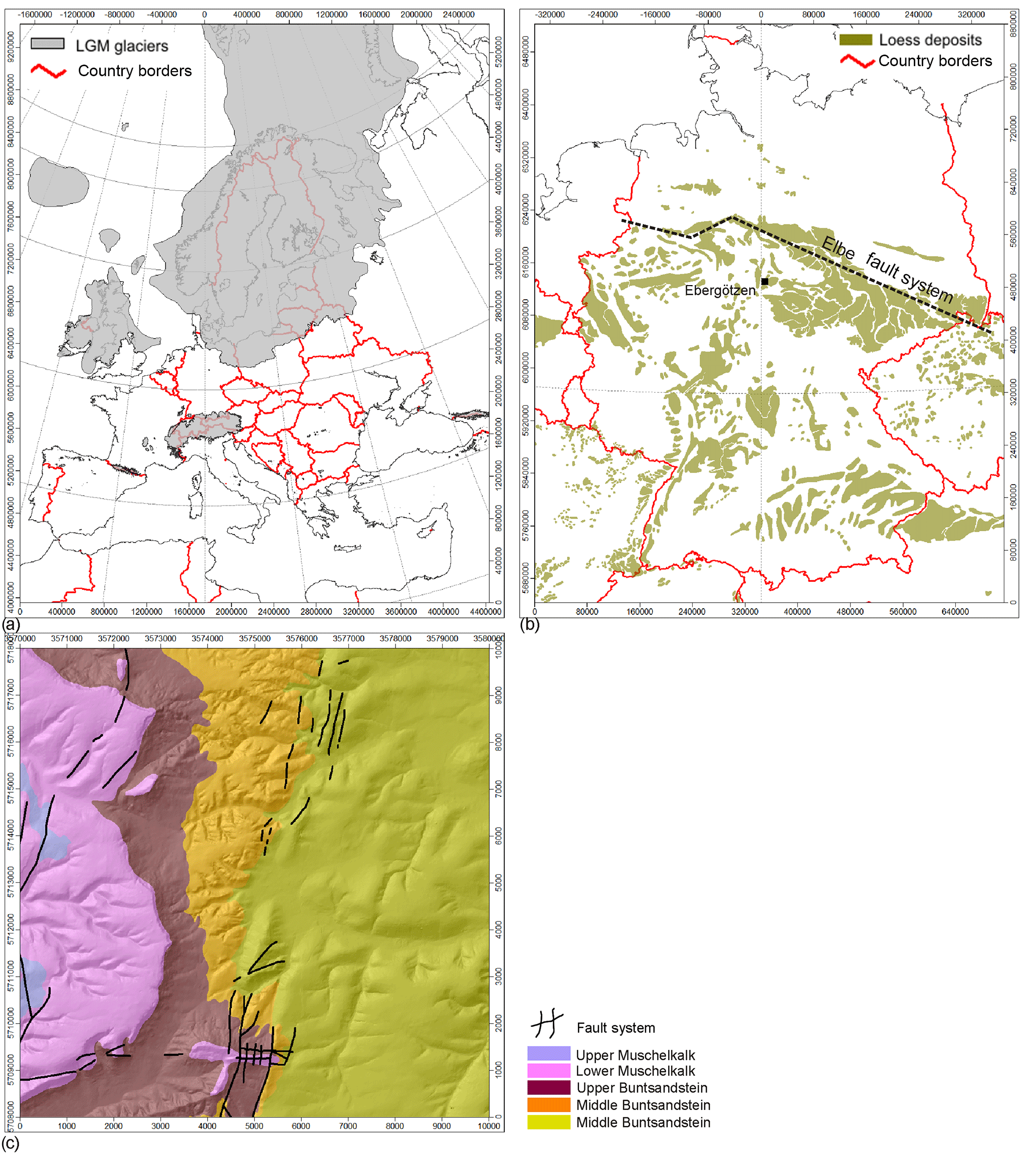
Figure 1 Location of the study site: (a) glacial ice sheets of the Last Glacial Maximum (20–18 ka BP) in Europe, data from Ehlers and Gibbard (2004); (b) loess deposits in Germany, data from Haase et al. (2007), test site at Ebergötzen as black rectangle; (c) simplified geological map of test site at Ebergötzen, according to Ehlbracht (2000). For our purpose, the areas with quaternary deposits were removed.

The study area is geomorphologically characterized by escarpments formed by Triassic sedimentary rocks of the Germanic Basin. The north German escarpment setting is shaped by NNE–SSW-striking major fault zones of paleozoic (Variscan) origin that were reactivated as sinistral transcurrent fault systems during Mesozoic (Alpidic) deformations (Mazur and Scheck-Wenderoth, 2005; Fig. 1b). Mesozoic transtensional deformations accompanied by salt tectonics led to development of half-graben structures and tilting of discrete upper crustal segments forming escarpments.

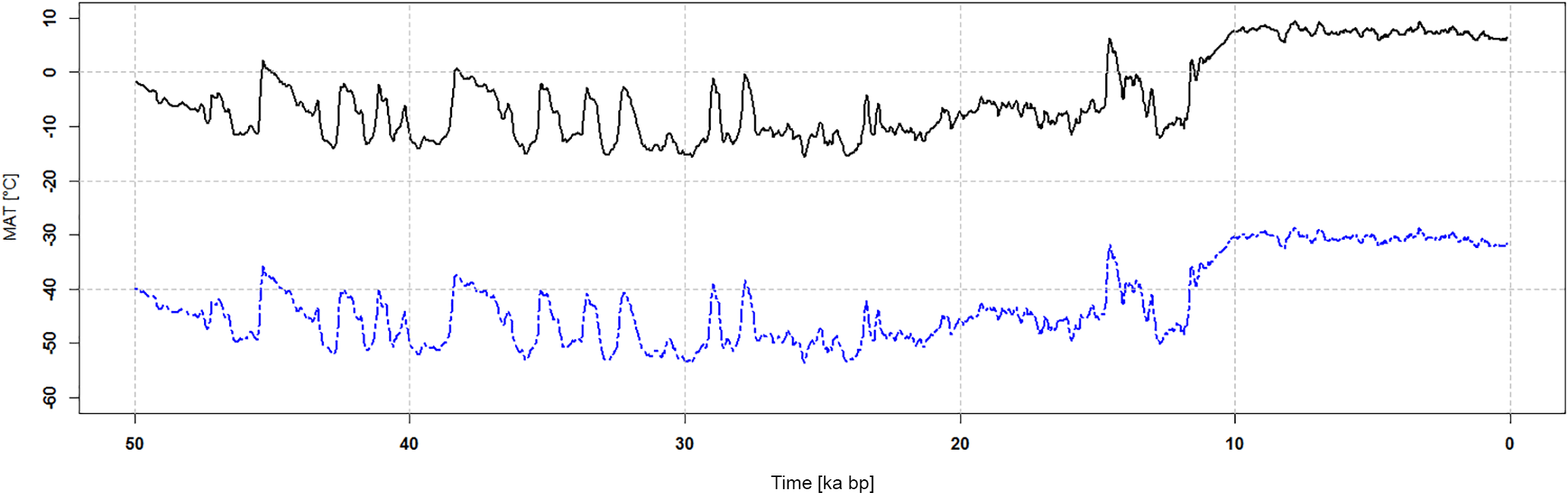
Figure 2 Derived mean annual temperature (MAT) data for the GISP2 location (dashed line) (after Alley, 2000) and the assumed curve for the test site at Ebergötzen (solid line).

Specifically, the study area of Ebergötzen (location in Fig. 1b, simplified geological map, Ehlbracht, 2000; Fig. 1c) is formed by two escarpments with corresponding flats and slopes. Roughly speaking, this can be described as follows:

• The western part of the area is dominated by a gently westward inclined surface built of Triassic limestones of the Lower Muschelkalk in relatively high altitudes (about 420 m above sea level). The Lower Muschelkalk is underlain by Lower Triassic claystones and siltstones of the Upper Buntsandstein that forms the escarpment of the Göttinger Wald.

• To the east, a slightly westward inclined surface (elevation about 290 m a.s.l.) consisting of red sandstones of the Middle Buntsandstein 2 is exposed. This surface is bordered by a steeply sloping section at the base of the escarpment which consists of sequences of sand- and siltstones of the Middle Buntsandstein 1.

• Further to the east, in general, the importance and thickness of loess rises, partly as insular very thick resources can be found (> 10 m).

During the glacial periods of the Pleistocene, the periglacial environment of our study site was characterized by intensive weathering, erosion and transport processes. Frost weathering of numerous freeze–thaw cycles resulted in loosening of the exposed sedimentary bedrock mainly along joint surfaces. Additionally, extensive dissolution of the calcareous rocks of the Muschelkalk fragmented these lithological successions. The crushed rock was released from the rock mass and – dependent on the local terrain situation – remained in situ or was moved downhill by solifluction, creeping and mass wasting processes. The intensity of the weathering processes as well as the speed of the transport processes depend on the material properties of the rock, respectively, rock debris but is also altered by allochthonous input of loess material. Figure 1b shows that the spatial distribution of loess deposits of different but considerable thickness is a general phenomenon in wide areas of Germany.

3 Materials and methods

The general purpose of LEM is a better understanding of landscape history through a simulation of land-forming processes and process interactions (Tucker and Hancock, 2010). The main purpose of SaLEM is the mapping of regolith properties according to known physical relationships. In the absence of reliable data for certain process variables, these have to be substituted by suitable parameterizations.

3.1 Methodological background

SaLEM has been developed using the SAGA framework, which is an open-source software that provides an extensive application programming interface dedicated to spatial data analysis and visualization (Conrad et al., 2015). SaLEM simulates the dynamics of selected landscape-forming processes (weathering, erosion, transport and deposition), thus representing an operational GIS tool for numerical process modeling. Differential equations used in the model are based on simplified physical models, such as the description of weathering or transport processes. The original C code of GOLEM (Tucker and Slingerland, 1997) was ported to the C$++$ based environment of SAGA. Tucker and Slingerland (1997) describe the aim of GOLEM as the exploration of the interaction of tectonics (uplift) and erosion for the landscape over long geological timescales (several Ma). The goal of SaLEM is the lithologically differentiated modeling of weathering, erosion, transport and deposition of unconsolidated material covering the bedrock for comparably shorter periods (recent 50–100 ka). The part of GOLEM that in particular is relevant for these objectives is the submodel for diffusive regolith creep. With the focus on the prediction of parent material for soil formation, it does not consider landscape compartments that are beyond this scope. Accordingly, the modeling of fluvial incision and transport as tectonic uplift was not adopted. GOLEM's function for regolith production (or weathering) was replaced by a set of rock-specific and climate-sensitive equations considering frost and chemical weathering separately. The simulation time is freely selectable and depends only on the availability of climate data, which are considered as highly evident to drive the model.

One problem for LEM-based forward modeling is the impossibility to reconstruct the initial palaeotopographic situation. This problem is known as equifinality or convergence of landforms and was discussed many times in geomorphographic papers (e.g., Odoni, 2007; Peeters et al., 2006). It must be considered highly evident when modeling over longer geological time spans (several Ma); however, for the period considered here (50 ka), it can be proposed as less important (Peeters et al., 2006). Therefore, we use the actual topography as predefined by the digital elevation model (DEM) for the initial topography of our modeling.

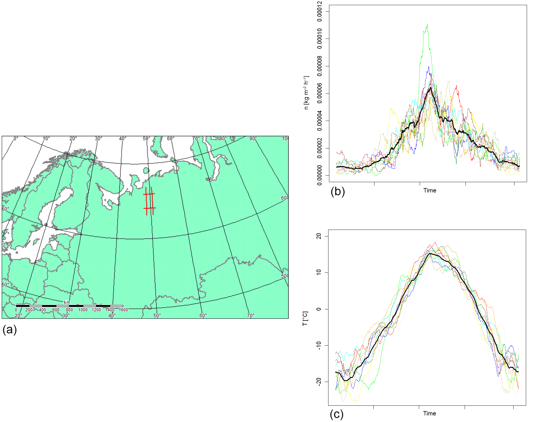
Figure 3 Location (a) and annual variations of precipitation (b) and temperature (c) for 9 years of the Timan Ridge, Russia, derived from NCEP/NCAR reanalysis data (Kalnay et al., 1996). The model uses the average curves (bold black line).

The layer of unconsolidated material, which today is omnipresent, covering the bedrock, is the result of various natural processes that interacted for many thousands of years. Solid bedrock is weakened by two categories of weathering processes: loosening of the rock mass by physical weathering and rebuilding of the mineral constituents by chemical weathering. When individual fragments are separated from the bedrock, the unconsolidated material (regolith) is exposed to downhill transportation by gravitational processes. During the late Pleistocene, discrete episodes of intense mixing of the unconsolidated layer with allochthonous materials are evident, in particular during the Middle and Upper Weichselian, when aeolian sediments like loess were accumulated and reworked with autochthonous material (Frechen et al., 2003). This took place under the influence of vegetation and resulted in several multi-material layers covering the solid rocks of the mountainous areas with a thin cover of regolith. The thickness of this coat may range from a few centimeters up to several meters. Due to its physicochemical properties, its proportion in regolith influences current soil properties significantly.

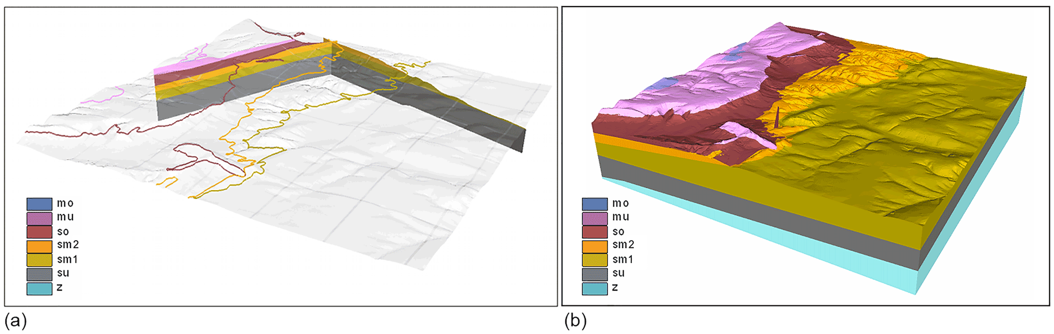
Figure 4 Geological units in the test site at Ebergötzen, elevation registered with the DEM data (b) and the geological cross sections (a) derived from Ehlbracht (2000): Upper Muschelkalk (mo), Lower Muschelkalk (mu), Upper Buntsandstein (so), Middle Buntsandstein 2 (sm2), Middle Buntsandstein 1 (sm1), Lower Buntsandstein (su) and Zechstein (z).

Basically, all weathering and transport-related processes follow physical and chemical laws that should be reflected by the model. However, this can only be done in an approximation to the real-world phenomena due to several reasons. Input data are not available for all factors of the involved processes, the spatial resolution is not applicable to model all processes realistically, and still physical modeling of some of the involved processes would be too complex and beyond the scope of SaLEM. Thus, modeling is limited to processes that can be depicted and empirically described. This general feature of reduction becomes especially clear in the case of modeling the periglacial layer as parent material, because many processes, such as the influence of vegetation on erosion, transport and allochthonous deposits, remain unconsidered.

3.2 Climate data

The climatic development of the Northern Hemisphere during the Pleistocene is fairly well known nowadays due to recent methodological developments in palaeoclimatology. Through the introduction of ice core analysis as proxies it became possible to reconstruct the course of long time series of climatic elements, although the derived information applies only to the locations where the data are taken from Bubenzer and Radtke (2007). Palaeoclimate modeling of global data records is now available in relatively high spatial and temporal resolution (e.g., Kageyama, 2017).

For the calibration of chemical and physical (frost) weathering, two climate data sets are considered: one for the long-term temperature signal and one as the scenario representing the annual/seasonal climate. The long-term signal has been taken from the ice core project GISP2 (Alley, 2000). It provides 30-year temperature averages for the last 50 000 years. These temperatures have been adapted to the annual mean temperatures of our study site. Figure 2 shows the course of temperature, which was derived for the location from the ¹⁶O ∕ ¹⁸O isotope ratio.

A total of 1631 values are available for a period of 50 000 years, which means an average of 30 years resulting in one mean temperature value. Although these are unevenly distributed (17 values for most of the past 1000 years and 115 values for most of the recent 100 years), the average period shown in the data is still more accurate than the required temporal resolution of the model which is conducted with a time step of 100 years at the moment. The curve ends up with the value of −31 ^∘C as the current mean annual temperature of the GISP2 location. SaLEM raises the entire curve to the actual mean annual temperature level (Ebergötzen, 8 ^∘C) of the respective working area via the user interface.

For the annual variation of the temperature signal, a temporal resolution of 6 h and spatial resolution of about 210 km temperature data were extracted from the global NCEP/NCAR reanalysis programme covering the last 40 years (Kalnay et al., 1996). From this data set, a time series of a recent periglacial environment (Timan Ridge, Russia) has been chosen to act as analogue for the annual Pleistocene temperature and precipitation pattern at our study site (Fig. 3). The average of nine annual variations of the NCEP/NCAR data was then referenced to each temperature datum of the calibrated GISP2 curve.

Both the GISP2 data for palaeotemperatures and the NCEP/NCAR reanalysis data including the annual variations of precipitation and temperatures are provided to the user of SaLEM. Via a temperature offset, the level of the GISP2 curve can be moved up or down to calibrate it to different sites.

3.3 Bedrock geology and weathering indices

SaLEM operates on a geological model consisting of elevation-registered grids representing lithological contacts and topography (DEM). For simplification, the model uses the current topography represented by a DEM (50 m spatial resolution) as the initial starting point. For our study, a geological subsurface model was constructed from geological map information (Ehlbracht, 2000), two geological cross sections, a deep borehole and DEM data (Fig. 4b). For model construction, first the outcrop lines of the geological units were elevation registered with the DEM data, and the geological cross sections were vectorized and transferred into 3-D space (Fig. 4a). Subsequently, geological surfaces were constructed with the outcrop line and cross section line data using the geomodeler GOCAD^® (Paradigm, 2015). Last, thickness raster data for each lithological unit were calculated on the same resolution as the DEM data and assigned to each geological unit. These data then serve as geometrical lithological input information for SaLEM.

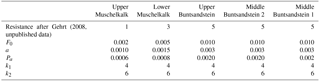
The weathering susceptibility of the different lithological model units was assigned through expert-derived chemical and physical weathering indices as proposed by Gehrt (2008, unpublished data) for the lithological successions of northern Germany. Gehrt (2008, unpublished data) arranged the 75 stratigraphic units occurring in Lower Saxony based on their resistance against weathering of their rock types at an ordinal scale (1: very resistant to 5: least resistant). Since the indices are not calculated from measured data, only the relative differences of the different rock types are used here. From this knowledge, the weathering equations adapted from Temme and Veldkamp (2009), were calibrated for each model time step to obtain the weathering rate through equations like the well-known “humped model” (for chemical weathering) inter alia. The applied weathering equations go back to Bloom (1998) (1), respectively, Cox (1980) (2):

$$\begin{array}{}\text{(1)}& {\displaystyle }{F}_{\mathrm{0}}\cdot {\displaystyle \frac{(T+(\mathit{\alpha }\cdot R\left)\right)-T_{max}}{(T_{min}-T_{max})\cdot \cos \mathit{\beta }}}.\end{array}$$

Equation (1) is for frost weathering in mm yr⁻¹, where F₀ is the maximum frost weathering on a flat surface, α is the buffering parameter for thickness of the regolith layer, R the thickness of the regolith layer, cos β is the cosine of slope, T is the mean annual average temperature (MAAT) in ^∘C, and T_max is the maximum MAAT, T_min is the minimum MAAT within the time step

$$\begin{array}{}\text{(2)}& -\left(P_{\mathrm{0}}\right(e^{-k_{\mathrm{1}}}-e^{-k_{\mathrm{2}}})+P_a).\end{array}$$

Equation (2) is for chemical weathering in mm yr⁻¹, where P₀ is the maximum chemical weathering rate, P_a is the chemical weathering in steady state, and k₁ is the weathering rate constant before the maximum rate is reached. With further increasing regolith thickness, the rate of chemical weathering decreases again; k₂ is the weathering rate constant after the maximum rate.

F₀, a, P_a, k₁ and k₂ are constants which are dependent on the material. In a lithological differentiated approach like SaLEM, the values for these constants were changed relative to each other according to Gehrt (2008, unpublished data) (see Table 1).

Table 1 Resistance against weathering (frost weathering and chemical weathering) of different triassic bedrock types occurring at the Ebergötzen site after Gehrt (2008, unpublished data) and derived initial values for the parameters of SaLEM's weathering (Eqs. 1 and 2).

3.4 Allochthonous deposits

One formative phenomenon of the periglacial deposits in central Europe is their partly large proportion of not in situ produced materials. These are designated as “allochthonous” materials consisting of the terrestrial, aeolian sediment loess.

In the absence of real measurement data describing spatially distributed loess deposition rates, a simple model was developed to indicate loess accumulation rates per year for each grid cell. These rates were derived from work done by Frechen et al. (2003), who calculated accumulation rates from loess profiles all over central Europe. The rates determined by Frechen et al. (2003) differ from 100 to more than 7000 g m⁻² yr⁻¹ for a period from 28 to 18 ka BP, respectively, 300 to more than 4000 g m⁻² yr⁻¹ for the period of 13–18 ka BP. To apply the discrete accumulation rates to the spatial SaLEM context, the SAGA module “wind effect” (Windward/Leeward Index; Böhner and Antonic, 2008) is parameterized on the basis of windward and leeward effects derived from a DEM taking into account a prevailing wind direction. In other words, the relief information is recalculated to index values dependent on the exposure to the assumed wind direction. As a prevailing wind direction during LGM in central Europe, the direction was set to ENE going back to Roche et al. (2007). The literature values for loess accumulation by Frechen et al. (2003) were translated in thickness per grid cell and stretched on the result of the index calculation (Fig. 5).

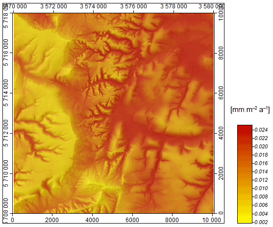
Figure 5 Parameterization of loess accumulation rate for Ebergötzen: DEM-derived parameter windward/leeward effect (Böhner and Antonic, 2008) combined with mass accumulation rates after Frechen et al. (2003) for the period of 28–18 ka BP.

For each time step in the modeling, the allochthonous input is simulated after the weathering process and before the downhill transport of the material. A spatially differentiated amount of loess material is accumulated on the grid cells. This information is passed to the model for each specific grid cell.

3.5 Transport

The simulation of hillslope sediment transport is modeled as a diffusion process, a concept that is commonly used for sediment flux modeling (e.g., Tucker and Slingerland, 1997; Pelletier, 2008; Anderson and Anderson, 2010; Gillespie, 2011). It relates to Fick's law of diffusion and is used to describe the sediment flow with dependence on time and slope gradient, and results in a rate of change in elevation, expressed as

$$\begin{array}{}\text{(3)}& {\displaystyle \frac{\partial h}{\partial t}}=k_{\mathrm{d}}{\mathrm{\nabla }}^{\mathrm{2}}h,\end{array}$$

where h is the elevation, t is the time, and k_d is the hillslope diffusivity coefficient, which determines the speed of the diffusive sediment transport. Because sediment fluxes should be restricted to the unconsolidated regolith cover, the maximum allowed rate of change in elevation has been limited to the regolith thickness. Here, SaLEM closely follows the original GOLEM implementation.

While the quantification of sediment transport and its associated denudation and deposition follows a well-established approach, it does not give information about the sediment composition. In order to overcome this restriction, we developed a tracer concept for the model. Such tracers represent soil particles, which are released and evenly distributed in the regolith layer. The information that a tracer stores is its geographical position, the depth at which it is buried and the geological unit from which it was released. The closer a tracer is to the surface, the higher is the probability that it becomes moved by diffusive hillslope transport. The decision if a tracer is moved in a simulation time step is made with a depth-dependent random function. If a tracer is moved, it follows the direction of the slope aspect. The covered distance is estimated as a function of slope and hillslope diffusivity coefficient. To reflect uncertainties in the tracer path simulation, a degree of randomness can be added to the direction, distance and depth at which it will be deposited again. For each tracer, its path can be stored in an additional data set. Further information can be collected about the time and the duration of its transportation (Fig. 6).

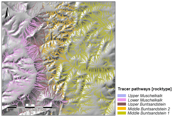
Figure 6 Transport pathways in Ebergötzen of the virtual tracer particles from the location of their release from the rock via weathering and erosion to the place where the transport stops.

3.6 Model run

A model run is executed for the specified time range using a discrete time step size, typically 100 years. Initializations done before the model run comprise the loading of the climate database, the validation of weathering equations and the depth of an initial regolith cover. Now,,,,, the same processing scheme is applied for each time step. At first, allochthonous input, if specified, is added to the regolith cover. This also increases the surface elevation. The next step is the bed rock weathering, which will increase the regolith cover without changing the surface elevation. The weathering rate depends on regolith thickness, climate variables and rock-type-specific equations. Weathering rates are determined in monthly steps for one annual scenario, thus reflecting seasonally changing weathering conditions, and then multiplied with the time step size. Finally, the diffusive hillslope transport is simulated.

The repetition of the subprocesses weathering, allochthonous supply, erosion, transport and accumulation leads to a growing regolith layer whose thickness in turn influences the weathering equations via the humped model: initially, the weathering rate intensifies; from a certain thickness on, it decreases again.

4 Results and evaluation

Regolith thickness has been estimated via simulation of processes such as lithologically differentiated weathering of bedrock, erosion, transport and accumulation, as well as loess material supply from the last 50 000 years. The modeling was carried out for three variants: without initial sediment cover (Fig. 7), with sediment cover of 50 cm thickness in general (Fig. 8) and finally with simulation of loess input (Fig. 9) according to accumulation rates proposed by Frechen et al. (2003).

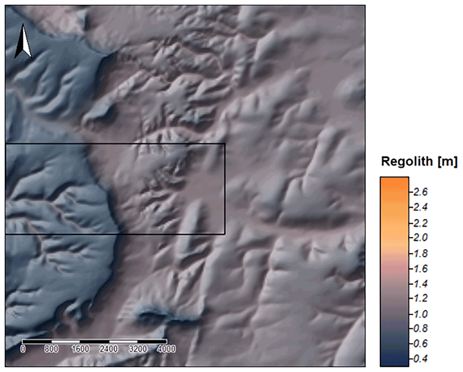
Figure 7 First results of the SaLEM simulation in Ebergötzen showing distributed regolith thicknesses resulting from 50 ka modeling. The rectangle indicates the area where a first validation of the results was conducted.

These modeling data provide a picture of the spatial differentiation of regolith thickness for the study area: valley areas are equipped with a massive filling up to several meters, whereas on ridges and near steep slopes the thickness of the regolith tends towards zero. To the east of the study area, the total thickness generally increases. Small tributary valleys have fillings thicker than the large main valley (in the center of the area), which drains to the east. Spatial differentiation within the slope areas clearly can be seen. This general picture is shown by all of the three variants; in detail, the three variants differ significantly.

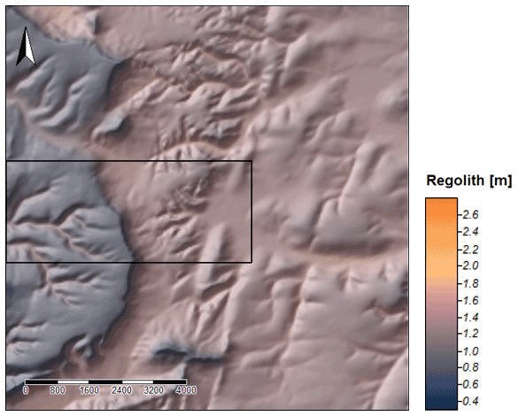
Figure 8 First results of the SaLEM simulation in Ebergötzen showing distributed regolith thicknesses resulting from 50 ka modeling with initial 50 cm regolith cover. The rectangle indicates the area where a first validation of the results was conducted.

Figure 9 First results of the SaLEM simulation in Ebergötzen showing the distribution of regolith thicknesses resulting from 50 ka modeling including allochthonous input (loess). The rectangle indicates the area where a first validation of the results was conducted.

Due to the lack of spatial data on properties of the regolith, the validation of the model results is challenging. To give a first impression, a compilation of available drilling point data from soil surveys is used to validate the trend of the results of the model regarding regolith thickness within a limited validation rectangle.

All available soil data for the area from the Lower Saxony State Office for Mining, Energy and Geology (LBEG) were collected (1141 point data within the validation rectangle; source: LBEG, soil profile database; Fig. 10). However, since these are manually collected data for soil mapping projects, in most cases, the total thickness of the regolith cover is not completely recorded. Therefore, the depth of the weathered C horizon was extracted for each profile although this value was set rather arbitrarily to 100 cm for many locations due to the applied method (manual drilling) which cannot drill deeper into the soil.

The depths of the C horizons of the profiles were averaged for different process areas separately for the stratigraphic units of the simplified geological map (Fig. 10, Elbracht, 2000, unpublished data) and for terrain positions of the simplified geomorphographic map (Fig. 12, LBEG and scilands GmbH, 2008, unpublished data) and then compared with the generated model data of the version with allochthonous input (Fig. 9), also averaged for the process areas.

Figure 10 Drilling points (n=1141) from LBEG soil profile database on the simplified geological units within the validation rectangle.

The trend read in the profile data could be confirmed: in the process area, which is defined by the occurrence of the stratigraphic unit of the Lower Muschelkalk limestone, the lowest average regolith thickness was modeled. For the three units of Buntsandstein, on the other hand, substantially higher mean thicknesses appeared. The modeled differentiation between Upper Buntsandstein, Middle Buntsandstein 1 and Middle Buntsandstein 2 could not be confirmed by the profile data because here the average values of all the units slightly fluctuate in a similar manner around at least the partly artificial maximum value of the profile depth (Fig. 11).

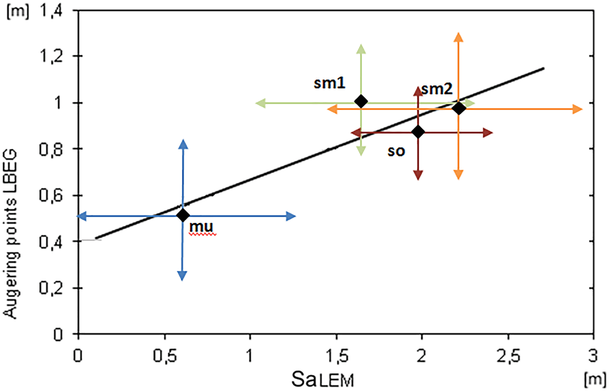
Figure 11 The average thickness values (m) of the augering points compared to the average values of the SaLEM model run within the geological units of the validation rectangle: Lower Muschelkalk (mu), Upper Buntsandstein (so), Middle Buntsandstein 2 (sm2) and Middle Buntsandstein 1 (sm1). The arrows indicate the standard deviation values of the respective data sets.

For the hierarchically higher units of the geomorphographic map (bottom areas, slopes and summit areas stand for the relative bottom, middle and top; Fig. 12), also the trends in the profile data are reproduced in the model data: the lowest mean thicknesses were measured and also modeled in the summit areas of the terrain, higher mean thicknesses in slope and bottom area positions (Fig. 13). The fact that most profile data were set to an artificial depth of 100 cm is even more evident here: for slopes and bottom areas, SaLEM clearly produces different average thicknesses; in profile data, this difference is far less obvious.

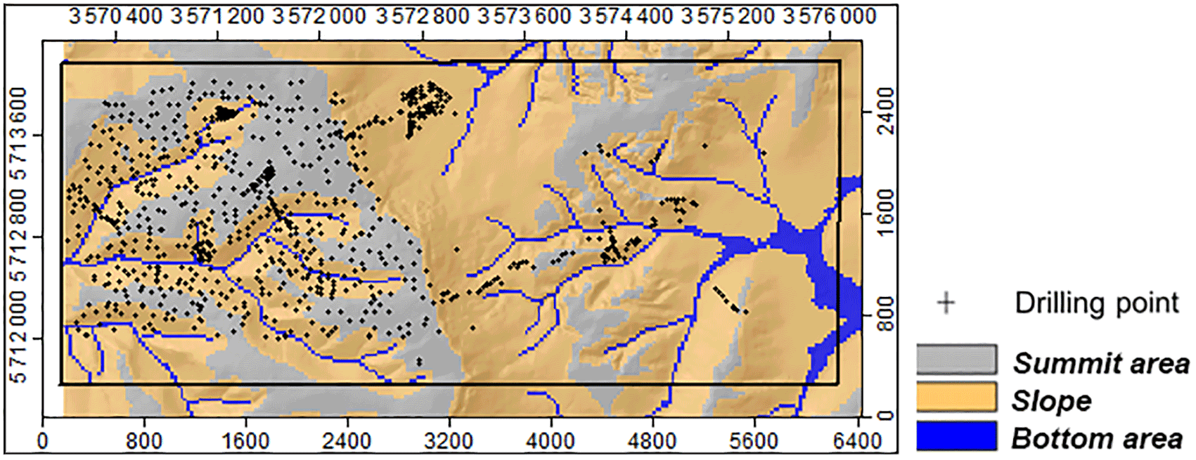
Figure 12 Drilling points from LBEG soil profile database on the units of the simplified geomorphographical map within the validation rectangle.

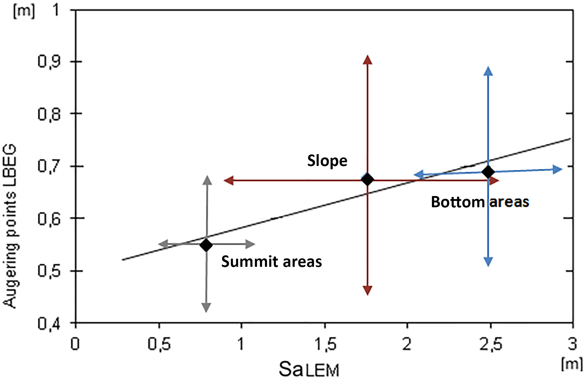
Figure 13 The average regolith thickness values (m) of the drilling points compared to the average values of the SaLEM model run within the units of the geomorphographical map of the validation rectangle. The arrows indicate the standard deviation values of the respective data sets.

The spatial differentiation of the model data within the individual process areas is not confirmed by the profile data. There are several possible reasons for this:

• The spatial resolution of 50 m grid cell size due to computing performance during the model development makes it impossible to reproduce the natural variability of regolith properties. Of course, the natural variability is present in the measured data points instead.

• The point data usually come with decimeter units; depths between full decimeters rarely occur. The focus is on the value of 100 cm, which was set when the hand drill device could not reach the final depth of the profile.

• The distribution of point data is not regular (Fig. 10). Approximately 74 % of all points are located in the area of the Muschelkalk limestone, corresponding to a point density of about 32 points per km²; only 15 % are in the area of the Upper Buntsandstein (point density of approximately 12 points per km²); only 9 % of the points fall into the Middle Buntsandstein 2 area (point density of 6 points per km²); in the Middle Buntsandstein 1 area, there is only 1 % (point density of 0.6 points per km² only). For the areas of the stratigraphic units of Buntsandstein, no spatial differentiation corresponding to the grid size of the model is possible.

As a further result, the transport distances as well as the spatial distribution of the various rock types are assessed (Fig. 6), which is simulated by the tracer pathways. The kilometer-wide paths of Lower Muschelkalk and Upper Buntsandstein material are regarded as particularly plausible in the thicker regolith cover of the valleys. These data will soon be validated by means of deep drilling, but their evaluation is not yet available.

5 Discussion and outlook

The landscape evolution modeling approach (review article; see Tucker and Hancock, 2010) we introduce here is to create spatially differentiated modeling data of soil parent material properties. To make things clear, it is not designed to explain the shape of a landscape as universal and comprehensive as Perron et al. (2012) did when he simulated the form of an entire landscape with its feathered valley networks. In this approach, we are looking into the recent past and start from an existing landscape to predict the properties of soil parent materials by simulating a set of processes involved.

Spatiotemporal modeling of these first-order processes of regolith formation in SaLEM makes use of known physical relationships if possible. When there are no data available for calculation of process variables, the modeling relies on parameterizations. For instance, data of climate variables are used for weathering equations; the weathering resistance of different rock layers instead is parameterized by rank data from Gehrt (2008, unpublished data). Another example is the assumption about the spatial pattern of loess accumulation rate, which is composed out of a DEM-derived index and the in situ loess accumulation rate determined by Frechen et al. (2003). In later phases of expansion of the model, these parameterizations might be substituted by measured data or data from other sources.

The process of regolith evolution during the LGM is a complicated intermeshing of many different subprocesses. With SaLEM, initial results are obtained with certain validity. However, SaLEM covers only a few subprocesses at this stage. We therefore have concrete ideas for the next steps.

In the near future, we will strive for more realistic parameterization of the weathering properties of the lithological units using field (rock mass strength) and laboratory data (mineralogy). This aims to objectify the assessment of the lithologically differentiated weathering resistance. We will further modify the transport functions for different lithological materials and elaborate a suitable approach to dynamically model textural changes in the regolith evolution. The latter is a challenge, especially for the computational implementation. We will lay emphasis on the calibration of the existing model parameters by considering the results of a deep drilling campaign conducted in 2012 and 2013. Unconsolidated fillings of valleys were sampled at different positions in the area. With these data, we have an occasional glimpse into regolith development. Another focus of future research will be the creation of validation data basis. Recent developments of non-invasive geophysical measurements give hope that at least for some areas we can generate validation data to prove our modeling results in the future. To reflect the recognition that also suddenly occurring events affect the evolution of regolith, we will incorporate existing models of discrete events (landslides, floods).