CIBUSmod 25.09: a spatially disaggregated biophysical agri-food systems model for studying national-level demand- and production-side intervention scenarios

CIBUSmod 25.09 is an open-source, spatially disaggregated biophysical model designed to evaluate resource use and environmental impacts in agri-food systems on national and sub-national level under future scenarios involving changes in demand and agricultural production systems. It provides a flexible, modular framework that can integrate regionalised data on crop and livestock production systems at the spatial resolution and aggregation level available. In the model agricultural production is distributed regionally to meet an exogenous demand, while enforcing several constraints that ensure internally consistent scenarios that are biophysically and agronomically feasible. Using Sweden as a case study, the model's application is demonstrated by constructing and validating a baseline and conducting a scenario analysis. The results highlight CIBUSmod's ability to quantify trade-offs in land use, nutrient flows, and greenhouse gas emissions across different transition pathways. The model is designed to be accessible, utilising Python and Jupyter Notebooks with Excel-based input data management. It is publicly available under the GNU GPLv3 licence. By enhancing transparency and usability in food systems modelling, CIBUSmod serves as a valuable tool for researchers to explore sustainable agri-food systems transitions at national and sub-national scales.

1 Introduction

Foresight studies and scenario analysis are valuable tools for studying different visions for future food systems, and identify synergies and trade-offs that can guide policy decisions under high levels of uncertainty (Reilly and Willenbockel, 2010; Woodhill et al., 2025). While scenarios can be purely qualitative, presented as narratives of possible futures, they are often combined with computational models to quantitatively assess their implications for key outcome variables (Riera et al., 2025; Reilly and Willenbockel, 2010). To support such analysis, numerous land and food system models have been developed, varying in scope, levels of detail, and complexity.

On a global level, integrated assessment models (IAMs) such as GLOBIOM (IBF-IIASA, 2023) and MAgPIE (Dietrich et al., 2019) have been extensively used to study effects on land use and greenhouse gas emissions under different Shared Socioeconomic Pathways (SSPs), feeding into multiple IPCC assessments. However, such models have been criticised for being opaque (Rosen, 2015) and inaccessible to large groups of researchers and practitioners (Jones et al., 2023). As a response to this, simpler biophysical mass flow models such as BioBaM-GHG (Kalt et al., 2021) and SOLm (Muller et al., 2017; Müller et al., 2020) at the global level, and CiFoS (Simon et al., 2024; van Zanten et al., 2023) at the European Union (EU) level, have been developed and used to study the biophysical feasibility of different future scenarios. Unlike IAMs, where supply and demand are calculated endogenously through economic modelling, based on price elasticities, these models determine demand from user input or by optimising diets to meet nutritional needs. Some of these models also allow the creation of large numbers of scenarios and scenario combinations to explore “biophysical option spaces” (Muller et al., 2017; Kalt et al., 2021). This could be the space of combined assumptions on future diets, productivity, land use, and more, that are biophysically feasible under different constraints.

For the purpose of national decision-making, however, these global-, or larger regional- (e.g. EU) scope models are not always adequate as they do not account for local nuances, policy priorities and knowledge. There is therefore a need for flexible models that can account for such local specifics. Recognizing this, the Food, Agriculture, Biodiversity, Land-use, and Energy (FABLE) consortium (Jones et al., 2023) has engaged researchers from diverse countries to develop national land-use and food systems pathways in collaboration with local stakeholders. These pathways are then globally aligned by balancing imports and exports iteratively, allowing for integration of local priorities alongside global food system sustainability goals. However, because the “FABLE Calculator” used for assessing country pathways operates at an aggregated national level, it cannot directly evaluate scenario feasibility or environmental impacts on sub-national levels (Jones et al., 2023).

In addition, several other national-scope biophysical models have been developed, often with a specific set of research questions in mind (see e.g. van Selm et al., 2023; Duffy et al., 2022; Karlsson and Röös, 2019). There is however a lack of flexible, open-source, spatially disaggregated modelling frameworks that operate nationally and sub-nationally with a comprehensive food systems perspective. To address this, CIBUSmod is introduced. It constitutes a relatively light-weight biophysical food systems modelling framework designed to incorporate detailed sub-national data and knowledge. It enables the evaluation of land use, material flows, and environmental impacts under different future food systems scenarios. Using Sweden as a case study, its applicability is demonstrated through data acquisition, validation, and scenario assessment. The model, CIBUSmod 25.09 (Karlsson et al., 2025), was built in Python and is made available as open-source under the GNU GPLv3 licence.

This paper is intended to act as a source of reference for future work as well as an introduction for new users. In Sect. 2, a description of CIBUSmod's general structure and different modules is provided. In Sect. 3, a use case example for Sweden is provided, describing data acquisition and model validation as well as providing an example of scenario simulation and assessment. Finally, in Sect. 4, the model's applicability and plans for future development are discussed. In addition, the public GitHub repository contains a user guide that focuses on the technical aspects of installing, setting up the Python environment, structuring input data, and setting up model runs.

2 Model description

CIBUSmod uses user-input on e.g. human diets, population size, and processing conversion efficiencies to calculate national demand for crop and animal products (including exports) and then meets this demand by distributing crop areas and livestock across a number of user-defined sub-national regions. This enables the use of sub-national data of arbitrary geographic resolution. The distribution of crop areas and livestock across regions is determined by solving a convex optimisation problem, which minimises deviation from a pre-defined initial state (e.g. the current distribution), while also enforcing constraints to ensure that the solutions are biophysically and agronomically feasible.

A key module of the model is the ParameterRetriever, which provides a flexible way to input data at different levels of specificity depending on availability, with the model automatically using the most specific data provided. Specificity refers both to spatial detail (i.e. from national average values to region-specific values) and to how parameters are defined across different categories, allowing them to be applied broadly or distinguished with finer resolution. For example, the parameter controlling the share of animal manure handled with different manure management systems could be specified broadly per animal species (e.g. the same distribution for all pigs) or with finer detail per production system and animal category (e.g. a specific distribution for organic sows) if data is available. All input parameters are provided through Excel workbooks, making the model easy to use without extensive programming knowledge. It allows users to add and parameterise additional food items, crops, and livestock production systems, to be able to address diverse research questions. Parameters are categorised into “default parameters”, which include the initial values required to run the model, and “scenario parameters”, which describe how these default values are expected to change over time under different scenarios. When designing scenarios, only parameters expected to change need to be specified. Unspecified parameters make use of their default values.

CIBUSmod uses primarily open-source Python packages and is ideally run via Jupyter Notebooks. This facilitates the documentation of model runs and the generation of output figures in a convenient and reproducible way. Output data is stored in an SQLite database, and the modelling framework provides tools for extracting, summarising, and visualising the model outputs.

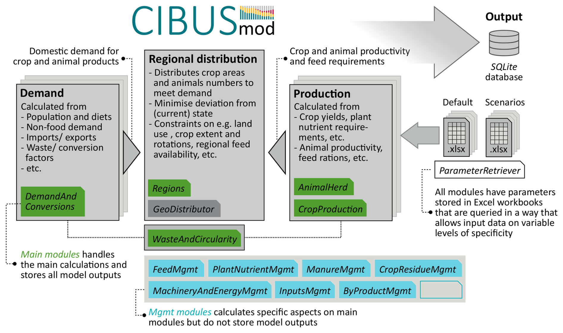
Figure 1 Schematic illustration of CIBUSmod model structure showing the calculation flow from accessing input data via the ParameterRetriever (right hand side) through calculating demand and production in the main modules (green boxes), and regional distribution via the GeoDistributor module (grey box).

The framework is modular, with independent components handling different parts of the calculations, which simplifies maintenance and allows for the incorporation of additional functionality by adding new modules. The modules are organised into “main modules”, which store all model output, and “management (mgmt) modules” that perform specific calculations without storing output data. Figure 1 provides an overview of the CIBUSmod modelling framework and its included modules.

The following sections describe all main components of the modelling framework and provide details on the steps involved in the different calculations.

2.1 Calculation of demand for agricultural production

Demand for agricultural production is handled with the DemandAndConversions module, which takes exogenous inputs of population size, national diets (including import shares and shares of food from different production systems such as organic or conventional agriculture) and demand for non-food and export uses. Diets are supplied in terms of food consumed (i.e. after accounting for all losses), which allows for assessing nutritional adequacy of supplied diets. The model uses supplied waste generation and conversion factors to calculate total national demand for crop and animal products, by-products and crop residues as well as generated by-products, wastes and import demand.

For dairy products, the model balances supply and demand for dairy fats. Domestic demand for high-fat products such as butter and cream may exceed the milk fat obtained as a by-product of producing low-fat products. In that case, the model increases low-fat (skimmed) milk powder exports by an amount sufficient to meet the excess demand for dairy fats.

In the current version of the model, the supply and demand for by-products is balanced in the ByProductMgmt module by adding additional imports of by-products if domestic supply does not meet demand for feed, food and non-food uses. Surplus by-products are either assumed to be exported or transferred to waste management (see Sect. 2.9), or a mix thereof, as specified through input parameters. This approach has some clear limitations, which are further discussed in Sect. 4.

2.2 Regional distribution of crop areas and animal numbers

Crop areas and animal numbers needed to meet calculated demand for agricultural products are distributed across regions by the GeoDistributor module. In the default case, crop areas and animal numbers are distributed by solving a quadratic optimisation problem with the goal function in Eq. (1):

$$\begin{array}{}\text{(1)}& min\sum {\left(f_{i,j}{x}_{i,j}-f_{i,j}x{\mathrm{0}}_{i,j}\right)}^{\mathrm{2}},\end{array}$$

where x_i,j and x0_i,j is the area or number of crop or animal i in region j of the solution and the initial state, respectively. The factor f_i,j is calculated from Eq. (2):

$$\begin{array}{}\text{(2)}& f_{i,j}={\mathrm{rn}}_{i,j}\times {\mathrm{sf}}_{i,j},\end{array}$$

where rn_i,j is a factor that normalises all features (i.e. distinct land use classes and animal species) based on the maximum x0 of each feature according to Eq. (3):

$$\begin{array}{}\text{(3)}& {\mathrm{rn}}_{i,j}={\displaystyle \frac{\mathrm{1}}{{max}_{i\in F,j}x{\mathrm{0}}_{i,j}}},\end{array}$$

where F is the set of all crops or animals i that belong to the same feature. This normalisation was introduced to account for the different units of measurement across features (e.g. hectares for crops, square meters for greenhouse crops, and headcounts for animals) and to prevent features with larger numerical values from being given disproportionately higher weight in the model. The scaling factor sf_i,j is calculated from Eq. (4):

$$\begin{array}{}\text{(4)}& {\mathrm{sf}}_{i,j}={\left({\displaystyle \frac{\stackrel{\mathrm{‾}}{x\mathrm{0}\times \mathrm{rn}}}{x{\mathrm{0}}_{i,j}\times {\mathrm{rn}}_{i,j}}}\right)}^{\mathrm{sp}},\end{array}$$

where $\stackrel{\mathrm{‾}}{x\mathrm{0}\times \mathrm{rn}}$ is the mean of all normalised x0, and sp is a parameter that controls the power of scaling; sp =0 means that the model aims to minimise deviation from the initial state in absolute terms. A larger sp gives increasing weight to relative deviations. Thus, a larger sp will result in larger absolute changes for crops, animals and regions where areas or animal numbers are large in the initial state. This scaling factor is introduced to give less dramatic changes in smaller regions. For example, in the case of a scenario where demand for a specific crop is reduced, sp =0 may result in areas going to zero in regions where that crop is grown on a small area in the initial state (i.e. result in a 100 % relative reduction). Increasing sp will penalise these relative deviations, which will result in larger absolute deviations in large regions while maintaining areas in the smaller regions. The selection of sp is an arbitrary choice that has to be made by assessing the plausibility of resulting land use patterns. In the model runs presented in this paper sp =0.4 is used throughout.

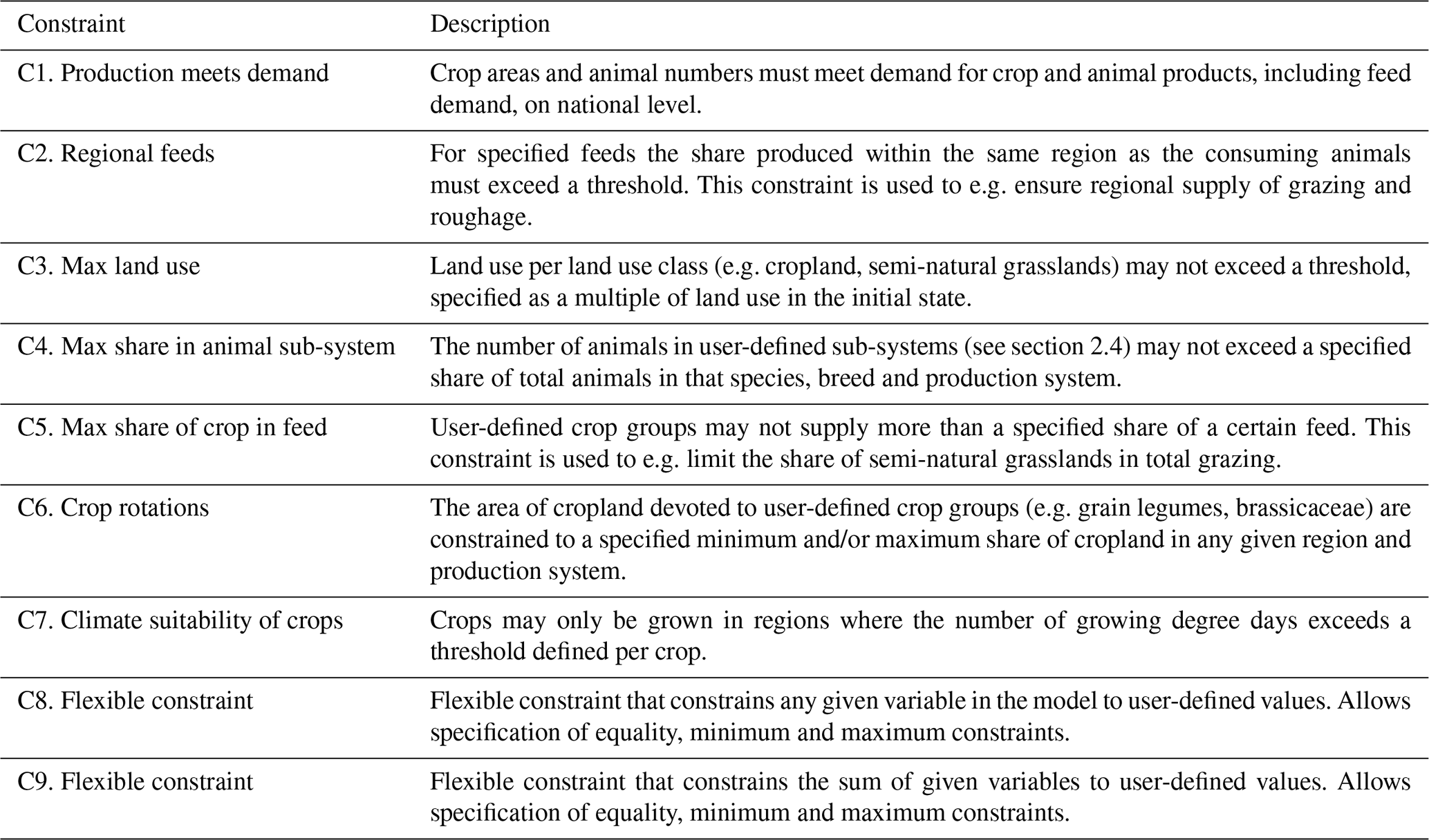
Table 1 Summary of constraints included in GeoDistributor module that distributes crop areas and animal numbers across regions in CIBUSmod.

It is also possible to supply a custom goal function as long as the problem remains convex. This allows users to study scenarios where, for example, land use is minimised or certain output from the system are maximised.

The optimisation problem is solved with the Python package cvxpy (Diamond and Boyd, 2016), using Gurobi (Gurobi Optimization LLC, 2024) as the default backend solver. The problem is solved under several constraints, summarised in Table 1. These constraints ensures biophysically and agronomically feasible solutions and allow for flexibility in deciding which constraints to include in a model run. The model also includes two categories of flexible constraints (C8 and C9 in Table 1) of which any number may be included in a model run to manually constrain solutions depending on specific research questions. In addition, it is also possible to programmatically construct additional constraints without changing the main code of the model as long as the problem remains convex.

2.3 Crop production systems

Crop production is handled with the CropProduction module, which calculates the mass of harvested crop products generated from cultivating a crop on a given area. Each production unit is specified by a crop, production system (e.g. conventional or organic), and region. The model allows for parametrising multiple crops used to produce the same product (e.g. winter and spring wheat) as well as a single crop used to produce multiple products (i.e. to represent intercropping). The main input to this module is crop yields, but it also takes input parameters for seeding density, above and below ground crop residues, crop nutrient contents, etc. This module allows specifying the maximum share of cropland that can be devoted to specific groups of crops in crop rotations, as well as the climatic requirements of different crops in terms of minimum number of growing degree days needed for a crop to be cultivated in a region. These parameters are used in the GeoDistributor (see Sect. 2.2) to constrain the regional distribution of crop areas.

2.4 Livestock production systems

Livestock production is managed through separate modules for each species and in some cases breed (Table 2). Currently, the model includes modules for cattle (dairy and beef), pigs, poultry (layers and broilers), sheep, and horses. Additional livestock modules may be developed to represent other species if needed for a specific use case. Each production unit is defined by a species, breed, production system, sub-system, and region, allowing for parameter settings at this specific level, or at a more general level. The `production system' attribute (e.g. conventional or organic) plays a central role in linking livestock product demand and feed supply. All feed for a given livestock unit must come from crops or by-products produced within the same production system. Similarly, the livestock products – such as milk, meat, or eggs – produced are used to meet the demand for foods from the same production system. The use of different sub-systems (e.g. ley or maize silage based dairy production or winter or spring lamb production) allows for further refinement, such as different rearing and feeding strategies or productivity within the same overall production system.

For each livestock production unit, the average number of live animals in a year, culled/lost animals, and the production of livestock products, are calculated based on parameters such as live weight gains, fertility, milk or egg yields, recruitment rates, mortality at different stages, and slaughter ages. The livestock production modules thus allow for a high degree of flexibility in parametrising different livestock production units (e.g. separate units representing dairy and suckler cow herds with their differences in feed requirements and production).

Table 2 Overview of livestock production modules and methods used to calculate feed requirements, manure excretion and enteric methane emissions.

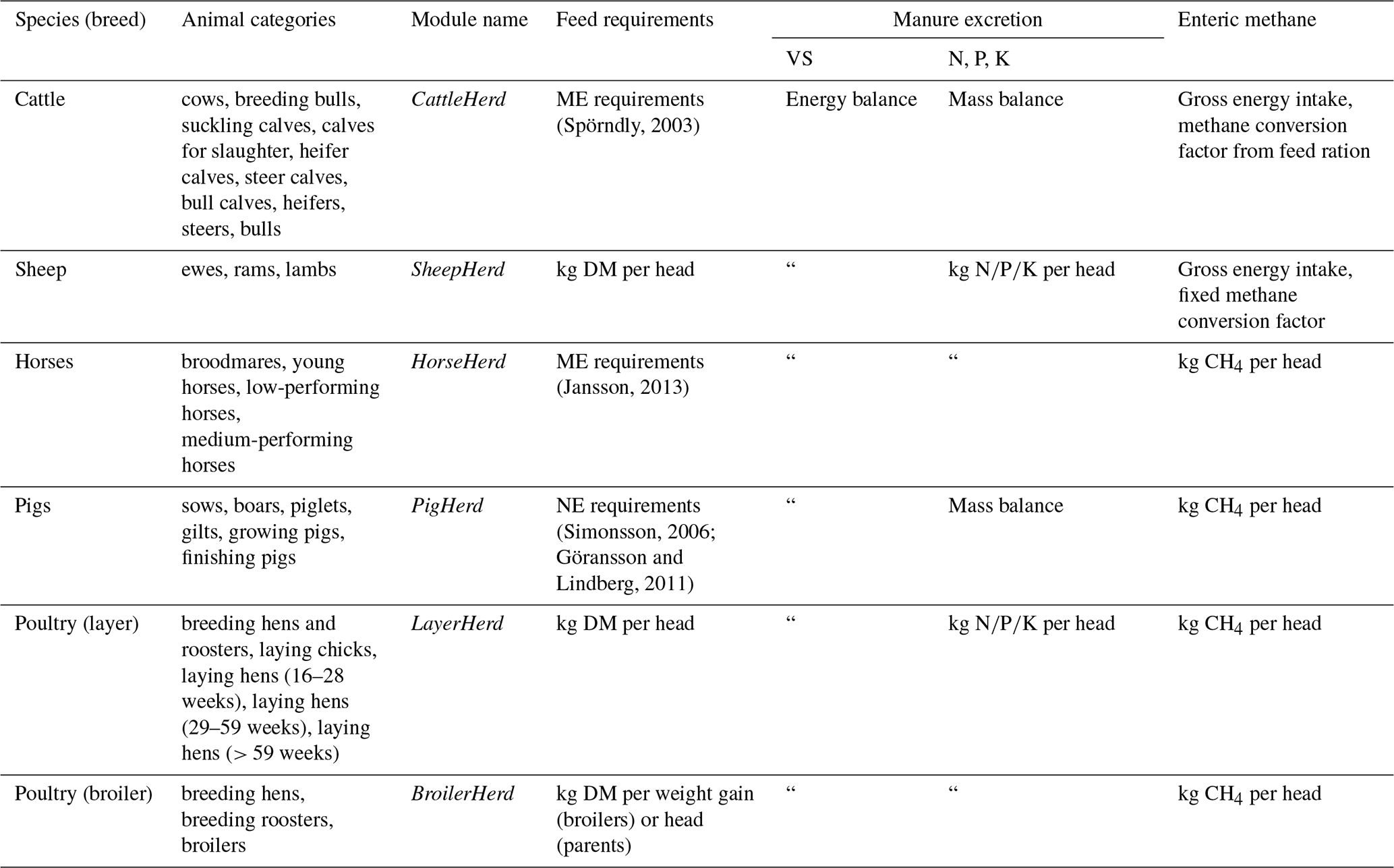
ME = metabolizable energy, NE = net energy, DM = dry matter, VS = volatile solids, N = nitrogen, P = phosphorus, K = potassium

2.4.1 Feed requirements and rations

Feed requirements, in terms of dry matter feed intake, are calculated per animal category based on either energy requirements, feed conversion ratios or a fixed dry matter feed intake per head. For cattle, metabolizable energy intakes are calculated based on the methods presented in Spörndly (2003), which include equations to calculate energy requirements for maintenance, growth, lactation, and gestation that can be parametrised to represent different breeds and production systems. For horses metabolizable energy intakes are calculated based on Jansson (2013). For sheep, feed intake is calculated from fixed factors for dry matter intake per slaughtered head of lambs or per head and year for other sheep. For pigs, net energy intakes are calculated based on the methods presented in Simonsson (2006) and Göransson and Lindberg (2011). For poultry, fixed factors for dry matter intake per head and year are used for laying hens and parent animals while for broilers feed conversion ratios (kg dry matter (DM) feed per kg live weight gain) are used to calculate feed intake.

Intakes of different feeds are then calculated in the FeedMgmt module based on exogenously supplied feed rations, expressed in terms of share of dry matter intake supplied from different feeds over a year, along with parameters for the energy density of different feeds. This module also calculates the nitrogen (N), phosphorus (P), and potassium (K) contents of the feed as well as enteric methane emissions.

Finally, feed intakes are translated to demand for domestic and imported crop and by-products using parameters for import shares as well as storage and feeding losses. Domestic crop product demand is handled in the GeoDistributor module during the balancing of demand and production (see Sect. 2.2). Parameters can also be supplied to enforce that a minimum share of demand for certain feed crops are supplied from within the same sub-national region as the consuming animals to e.g. ensure that there is regional supply of roughages.

2.4.2 Enteric methane emissions

For cattle and sheep, enteric methane emissions are calculated based on gross energy intake and methane conversion factors. For sheep, fixed methane conversion factors are used, analogous to the Tier 2 methodology presented in IPCC (2019), while for cattle, methane conversion factors are calculated based on feed ration composition according to the methodology presented in Bertilsson (2016), representing a Tier 3 methodology. For other livestock species, enteric methane emissions are calculated from fixed emissions factors per head as in the Tier 1 methodology in IPCC (2019).

2.5 Manure management

Calculation of manure generation and losses are handled within the ManureMgmt module.

2.5.1 Manure excretion

Excretion of volatile solids (VS) in manure are calculated through an energy-balance approach using Eq. (4), which is based on the Tier 2 method in IPCC (2019), together with total DM feed intake per animal (Sect. 2.4.1) and parameters on gross energy (GE) and digestible energy (DE) contents of the different feeds.

$$\begin{array}{}\text{(5)}& \mathrm{VS}=\left[\mathrm{GE}-(\mathrm{DE}+\mathrm{GE}\times f_{\mathrm{UE}})\right]\cdot \left({\displaystyle \frac{\mathrm{1}-{\mathrm{ASH}}_{\mathrm{rat}}}{{\mathrm{GE}}_{\mathrm{rat}}}}\right),\end{array}$$

where VS is volatile solids excretion per animal (kg head⁻¹ yr⁻¹), GE is gross energy intake from feeds (MJ head⁻¹ yr⁻¹), DE is digestible energy intake (MJ head⁻¹ yr⁻¹), f_UE is the fraction of urinary energy of GE intake (set to 0.04 for ruminants and horses; 0.02 for pigs), ASH_rat is the share of ash in the feed ration (kg kg DM⁻¹), and GE_rat is the gross energy in the feed ration (MJ kg DM⁻¹).

For poultry, apparent metabolizable energy intake from feeds (AME; MJ head⁻¹ yr⁻¹) are used instead of $(\mathrm{DE}+\mathrm{GE}\times f_{\mathrm{UE}})$ in Eq. (4). This directly represents the gross energy in feeds minus energy in faeces and urine (Abdollahi et al., 2021).

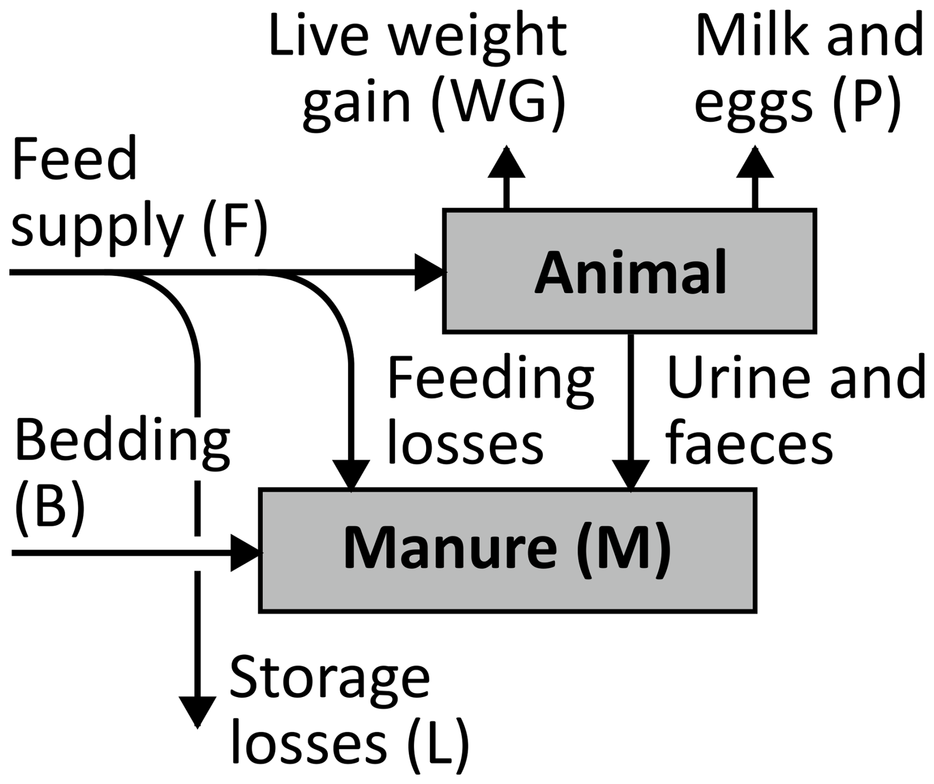
Figure 2 Schematic illustration of mass-balance for calculating nitrogen (N), phosphorus (P) and potassium (K) excretion in manure. $\mathrm{N}/\mathrm{P}/\mathrm{K}$ excretion is given by the equation M = F + B − L − WG − P.

Excretion of N, P and K are estimated from either: fixed excretion factors per head and year in line with the Tier 1 or 2 methodology in IPCC (2019), or from a mass-balance-calculation based on the methodology described in Statistics Netherlands (2012). The mass balance approach (Fig. 2) is used for livestock modules that explicitly calculates live weight gains for each animal category. Currently that includes cattle and pigs, which are the two largest contributors to manure excretion in many EU countries (Köninger et al., 2021). Excretion of N, P and K in manure is then calculated by summing inputs in the form of feed and bedding materials and subtracting outputs and losses in the form of feed storage losses, live weight gains and livestock products (i.e. milk and eggs). Nutrient contents of feed supply is calculated in the FeedMgmt module (Sect. 2.4.1) and nutrient concentrations in live weight gain for different animal categories and livestock products are supplied as parameters.

2.5.2 Storage emissions and losses

After calculating manure excretion, parameters are used to fractionate the generated manure from each livestock production unit across different manure management systems (e.g. liquid manure, solid manure, and deep litter) with distinct parameters for calculating losses in stables, storage, and during application.

Losses of methane (CH₄) during manure storage are calculated from VS in excreted manure (Sect. 2.5.1) and specified methane conversion potentials (B₀) and methane conversion factors (MCF) as per the IPCC (2019) Tier 2 methodology for all livestock categories. Total carbon (C) losses are calculated based on the C content in manure VS and a C loss factor, both of which are supplied as parameters. All parameters can differ across animal categories and manure management systems. The difference between total C losses and CH₄-C losses are assumed to be carbon dioxide (CO₂).

The calculation of N, P and K losses is performed by applying loss factors, representing the proportion of each element lost in stables and during storage. This approximately corresponds to the Tier 2 methodology for manure management in the EMEP/EEA air pollutant emission inventory guidebook (European Environment Agency, 2023). However, an explicit balance for total ammoniacal nitrogen (TAN) is not implemented. Loss factors can be specified per emitted compound, manure management system, animal type, etc. For N, factors can be specified either as a share of total N or TAN, depending on available data.

After determining all losses, these are subtracted from the excreted amounts to calculate the remaining C, N, P and K in the manure that is available for spreading on fields. This mass-balance approach ensures that nutrient availability for agricultural use is accurately modelled, reflecting different management practices and loss processes.

2.6 Plant nutrient management and liming

Calculation of N, P and K requirements for different crops as well as distribution of available animal manure and other fertilisers are handled with the PlantNutrientMgmt module. This module also calculates lime requirements and application, as well as nutrient emissions into the environment from fertiliser, manure and lime application, soil processes and leaching.

2.6.1 Crop nutrient requirements

Crop N input requirements are calculated in terms of kg plant available N per hectare from a second order polynomial equation, using the crop yield in tonnes per hectare as a variable and coefficients that can be specified per crop, production system, region, etc. Data for deciding the equation coefficients are e.g. national fertiliser recommendations and depending on data availability some coefficients may be set to zero to model requirements from a linear function of yield or as a fixed per hectare requirement. After calculating the requirements, these are met through a combination of residual N from crops (i.e. N released to consecutive crops in rotation) and application of manure and other fertilisers (see Sect. 2.6.2). The amount of residual N from crops is given as parameters in terms of kg residual N per hectare for different crops. As such, N fixation is not explicitly modelled in the current version but is indirectly accounted for in setting parameters for N requirements and residual N, making it possible to e.g. model green manure crops.

Crop P and K input requirements are calculated in a similar fashion as N requirements but only allow for a linear relationship with yield. Requirements can also depend on the stocks of P or K in the soil which can be specified per region. P and K requirements also allow for specifying an adjustment factor to account for e.g. uneven distribution of manure and intra-regional variation in soil $\mathrm{P}/\mathrm{K}$ stocks, leading to regional over-application compared to the requirements estimated from fertiliser recommendations.

2.6.2 Allocation of manure and other fertilisers

To quantify manure application and mineral fertiliser requirements, plant nutrients (N, P and K) in manure available for spreading are calculated as described in Sect. 2.5. A stepwise procedure is then used to distribute manure across crop areas. First (1), manure deposited while grazing is distributed based on the share of grazed biomass from different crops. Then (2), manure produced in organic animal production systems is distributed to organic crop areas within each region, based on plant available N requirements (see Sect. 2.6.1). For manure and other organic fertilisers, the plant available fraction of N is assumed equal to the TAN fraction. Then (3), manure produced in conventional animal production systems is distributed to organic areas within the same region it is produced, up to a maximum share of plant available N requirements, reflecting the share of organic N inputs originating from non-animal manure sources (e.g. municipal and slaughterhouse wastes). Then (4), manure remaining in conventional animal production systems are distributed to crop areas used for feed in the same region, and finally (4), any remaining manure in a region is distributed to conventional areas within the same region.

After accounting for TAN and long-term N release from applied manure, residual plant available N requirements are used to allocate other organic fertilisers (e.g. biogas digestate) across crop areas. The total amount of organic fertiliser available is calculated in the WasteAndCircularity module (see Sect. 2.9). The allocation procedure follows a similar logic as for animal manure: (1) organic fertilisers produced in each region are first applied to organic crops within that region; (2) any surplus is then distributed nationally to organic crop areas; (3) remaining amounts are allocated to conventional crops regionally; and (4) any final surplus is distributed nationally to conventional areas.

P and K in manure and other organic fertilisers are distributed proportionally to the N distribution (i.e. if 5 % of N in cattle manure in a region is distributed to a certain crop 5 % of P and K in cattle manure is also assumed to be distributed to that crop).

Finally, remaining N, P and K requirements are met through mineral fertiliser inputs. Thus, the model endogenously calculates mineral fertiliser use based on crop requirements, residual N from crops in rotation, and availability of manure and other organic fertilisers.

2.6.3 Lime application

Requirements for lime are calculated based on the acidifying or liming effects of N, P and K fertilisers and manure application as well as the excess alkali of harvested crop products and residues removed from the fields (Sluijsmans, 1966; Persson, 2003). For each item, parameters are supplied for their liming (or acidifying) effect in terms of calcium oxide (CaO) equivalents per kg N, P or K in fertilisers or manure, or per kg dry matter for crop products and residues. In order to calculate the total use of different liming agents, parameters are also supplied for the shares of different liming agents used and their respective neutralising value relative to CaO.

2.6.4 Emissions to the environment from fertilisers, manure and lime

NH₃-N losses from fertilizer and manure applications are calculated using emission factors per kg of N (or per kg of TAN for manure) as outlined by Swedish Environmental Protection Agency (2023a). These emission factors are provided as parameters and vary by fertiliser type, manure management system, and animal type. N₂O-N emissions are estimated according to the IPCC (2019) methodology, where N additions from fertilisers, manure, other organic fertilisers, and crop residues (both above and below ground) are multiplied by an emission factor representing the proportion of N emitted as N₂O.

The calculation of N quantities in applied fertilisers and manure is detailed in Sect. 2.6.2. N content in crop residues, both above and below ground, is estimated based on crop yield, residue production per harvested crop, and the N content of residues, all supplied as parameters. For crops that are not harvested such as fallow and green manures, a potential yield is specified and used to quantify generated crop residues. For above-ground residues, the amount removed is estimated based on the demand for crop residues as bedding material (calculated in the AnimalHerd modules) and for other uses (specified in the DemandAndConversions module).

N₂O emissions from cultivated organic soils are calculated by applying emission factors per hectare to the share of cropland on organic soils, as specified in the Regions module.

In the current model version, leaching is only considered for N, calculated as a specified proportion of N in organic and mineral fertilisers and crop residues that is assumed to leach according to the IPCC (2019) Tier 1 approach. Indirect N₂O emissions from deposition and leaching are not calculated directly in CIBUSmod outputs but are addressed in subsequent impact assessment stages.

Lastly, CO₂ emissions from liming are estimated based on quantities of applied lime (see section 2.6.3) and emission factors per liming agent in accordance with the IPCC (2019) Tier 1 methodology.

2.7 Energy use in agriculture

Agricultural energy use is handled with the MachineryAndEnergyMgmt module, which calculates energy use for field machinery, grain dryers, greenhouses and animal stables. This module also calculates emissions from fuel combustion. For each energy-using activity, the model allows specifying the share of energy from different sources, such as diesel or biodiesel for field machinery, or fuel oil, biofuels or electricity for animal stable heating.

Energy use for different field operations is calculated either from power calculations, where energy requirements for tractor and implements are calculated separately based on equations in ASABE (2006) and Robert Bosch GmbH (2014), or from fixed factors for energy requirements per hectare and/or harvest mass for different field operations. The former method is used for soil texture dependent operations, such as ploughing, harrowing and cultivation, thus accounting for regional differences in soil texture when calculating energy requirements. In both cases the useful energy at the implement is calculated first, after which an efficiency factor that accounts for losses in the power take-off, drivetrain and engine is applied to calculate the total gross energy required in the form of fuel. This allows to parametrise alternative drivetrains such as electric or hydrogen fuel cells. After calculating the total energy use for different field operations, these are multiplied by the number of times a specific field operation is performed for a given crop and production system, which allow for e.g. distinguishing between organic and conventional agriculture in terms of machinery operations, or modelling effects on energy use from implementing low/no-till systems.

To estimate the energy used for manure application, the total cropland area that receives manure is calculated. Then, specific factors for useful energy required per hectare are applied. The total cropland area receiving manure is calculated in the PlantNutrientMgmt module based on a user-specified minimum share of N that must come from manure where applied. For example, if a crop requires 100 tonnes of N in total, with 50 tonnes provided by manure, and the minimum share of N from manure is set at 75 %, then 67 % of the crop's total area will be assumed to receive manure (50/(100 × 0.75) = 0.67). This approach allows energy use for manure application to follow directly from the amount of manure generated in different scenarios.

Energy use in grain dryers is calculated based on the useful energy required per kg water removed, dryer efficiency and water content at harvest and after drying for different crops, as well as a factor for auxiliary energy requirements. For greenhouses, energy requirements are calculated based on user-specified energy use per square meter for different crops. Energy use in animal stables is calculated by specifying energy use per head, per inserted head or per unit of production or a combination of those. This allows the incorporation of varying datasets where the energy use is expressed in different terms. It is also possible to disaggregate stable energy use by specifying sub activities such as stable heating, stable machinery, or stable lighting which can have different mixes of energy sources.

2.8 Supply chain emissions from energy carriers, fertilisers and other inputs

To account for environmental impacts incurred throughout the supply chains of inputs used, the InputsMgmt module can connect each input to an Ecoinvent process and automatically retrieve inventory data. The connection to Ecoinvent is handled with the ecoinvent-interface Python package (https://pypi.org/project/ecoinvent-interface/, last access: 3 June 2025) and requires an Ecoinvent account with access to the database. It is also possible to manually specify emissions from inputs when a suitable Ecoinvent process is lacking. Currently the inputs accounted for in the model are all the energy inputs (e.g. electricity and diesel), N, P, and K fertilisers and lime.

2.9 Waste management and circularity

The WasteAndCircularity module manages the treatment of generated waste and losses. This module accounts for food waste and losses occurring at processing, retail, and household stages, culled animals, surplus by-products (i.e., instances where by-product generation exceeds demand for food and feed), and animal manure sent to centralised treatment. For surplus by-products, users can specify the proportion directed to waste treatment versus export in the ByProductMgmt module. The WasteAndCircularity module can also handle the treatment of non-waste biomass for bioenergy production, such as through anaerobic digestion.

For each waste fraction and non-waste biomass type, the proportion processed by different waste treatment methods is specified in the input parameters. So is the N, P, K and VS content of each waste fraction.

Calculations for different waste treatment methods are managed by dedicated functions. Currently, functions for anaerobic digestion, incineration, and landfill are included. Each function calculates (as applicable) the generated and used energy, the N, P, K, and C losses (e.g. in the form of NH₃, N₂O and CH₄) to the environment, and the N, P, K and C content in the generated organic fertiliser available for application to agricultural land. The allocation of generated organic fertilisers is handled in the PlantNutrientMgmt module (see Sect. 2.6.2). The WasteAndCircularity module is also designed to allow easy, programmatic addition of custom functions for new waste treatment methods without altering the main model code.

3 Application to a case study – Sweden

This section provides an example application of CIBUSmod on a case study, focusing on the Swedish agri-food system. In Sect. 3.1, the baseline data collection and validation is described, and in Sect. 3.2 the results from modelling two future scenarios using CIBUSmod, is presented.

3.1 Input data and baseline validation

Input data for the baseline were collected for the years 2016–2020. When available, a 5-year average for 2016–2020 was used. When data was not available for the entire country or time period, estimates from single case-studies or older data was used. Data were compiled from national statistics, statistics from industry organisations, published reports and peer reviewed publications. The following sections briefly describes the main data sources used in the different modules of CIBUSmod and provides validation of key output variables against previously published estimates and national statistics. The baseline dataset for Sweden, with references to data-sources, is provided open-source together with the model code in the model's GitHub repository.

3.1.1 Demand for agricultural production and process conversion factors

Swedish food consumption of approx. 70 food items (for the year 2020) was estimated from national statistics (The Swedish Board of Agriculture, 2024) and FAOSTAT food balance sheets (FAO, 2024). Import shares were taken from Schwarzmueller and Kastner (2022) for most products, and national statistics (The Swedish Board of Agriculture, 2024) for dairy products. Factors for food waste at processing, retail, and household stages, were based on estimates from Gustavsson et al. (2011) and conversion factors for translating food consumption (as eaten) into demand for raw agricultural commodities and associated by-product generation rates, were sourced mainly from FAO (2000). Organic proportions in consumption for most foods were obtained from Swedish organic food industry statistics (Swedish Organic Farmers Association et al., 2022), and in some cases adjusted to match production data according to national agricultural statistics (The Swedish Board of Agriculture, 2024).

3.1.2 Crop production

The model was parametrised with around 60 crops, covering major cereals such as winter wheat and spring barley, forage crops like ley for silage or grazing, four classes of semi-natural grasslands, grain legumes, rapeseed, as well as various horticultural crops, greenhouse cultivated crops, and fruit trees. The areal extent of different crops used in the optimisation goal function (see Sect. 4) was based on data from the Land Parcel Identification System (LPIS), provided by the Swedish Board of Agriculture, aggregated over “harvest regions”. These regions subdivide Sweden into 106 agronomically uniform areas which represent the smallest spatial scale on which national agricultural statistics on e.g. yields are presented. This is also the geographic scale used in the model for the case study. The LPIS data was further treated to disaggregate horticultural crops (presented as one category in LPIS data) to individual crop types and to separate conventional and organic areas. This was based on publicly available statistics on larger regional level or national level from The Swedish Board of Agriculture (2024).

Crop yields were estimated from the Swedish Board of Agriculture's statistics on “harvest region” level, where available. For many crops and regions, however, yield data is unavailable at harvest region level. In these cases, yields were extrapolated based on data from larger spatial scales (such as county, or national levels), along with a “reference crop” with good data coverage (usually spring barley). This method generates yield estimates for every crop across all regions. For crops with limited data, the extrapolated yields are highly uncertain. However, because the model allocates crops based on their current distribution, regions with more available yield data typically have much larger cultivated areas, which limits the impacts of this uncertainty.

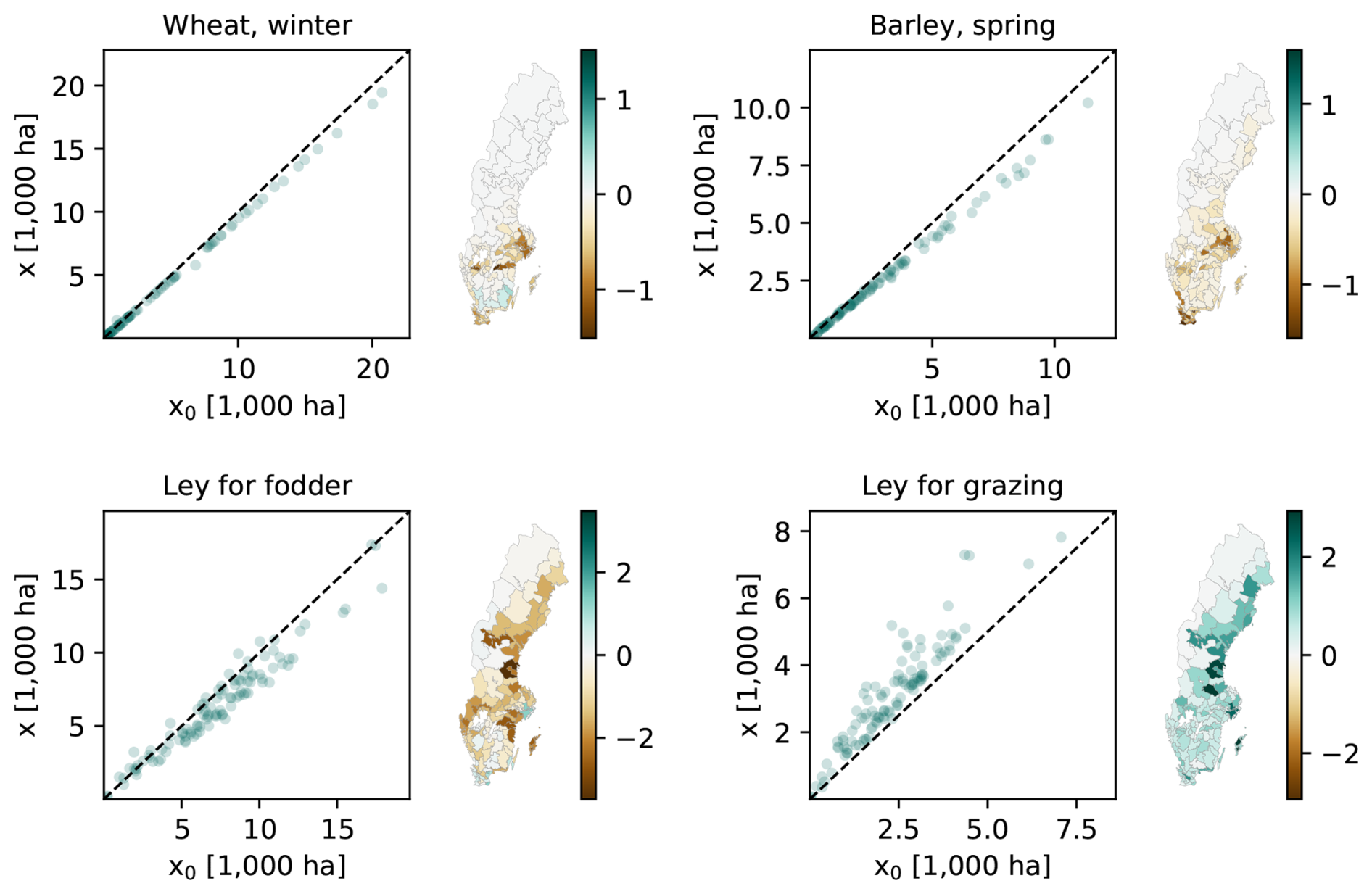
Figure 3 Regional distribution of crop areas in CIBUSmod (x) compared to crop areas estimated from national statistics and LPIS data (x₀). The dashed lines shows the 1:1 lines. The maps show x – x₀ per region.

Figure 3 shows the modelled distribution of four major crops compared to the current distribution based on LPIS data. For the two cereal crops, the model closely matches the current distribution, though with a slight underestimation in total demand. This leads to an underestimation of areas in the key cereal-growing districts in central and southern Sweden. The distribution of leys shows greater discrepancies. These are due to constraints that require at least 95 % of forage crops to be produced in the same region as the animals consuming them. It is an indication that forage crops and/or animals are likely moved across regional borders to a larger extent than allowed under the set constraints. Additionally, the model overestimates the area of grazed leys and underestimates leys for fodder production, particularly in northern Sweden. This discrepancy arises from the shorter grazing season in northern Sweden, which reduces the share of grazing in local feed rations. Since feed rations are currently implemented as national averages in the input data, regional differences in grazing periods are not captured.

3.1.3 Livestock production

The number of animals in each region was estimated based on national statistics, providing animal counts per municipality in June (The Swedish Board of Agriculture, 2024). These counts were then distributed over to the “harvest regions” using area overlaps to create the initial state used in the optimisation goal function (see Sect. 4).

Livestock productivity parameters, including fertility, slaughter ages, slaughter weights, and mortality, were sourced from national statistics, published papers, and reports. For cattle, data primarily came from Växa cattle statistics (http://www.vxa.se/statistik, last access: 3 June 2025), Einarsson et al. (2022), and Ahlgren et al. (2024). For sheep, Ahlgren et al. (2024) was the main source. For pigs, data were taken from Gård and Djurhälsan's WinPig statistics (https://www.gardochdjurhalsan.se/winpig/, last access: 3 June 2025), Landquist et al. (2020), and Zira et al. (2021). For broiler chickens, data were mainly sourced from Edman et al. (2022) and for laying hens data were sourced from Sonesson et al. (2008) and Carlsson et al. (2009). Animal feed rations were also gathered from the above mentioned sources, but for cattle and horses the concentrate component of animal diets was adjusted based on national feed industry statistics.

Overall, the estimated number of animals and their regional distribution closely match the statistics on animal numbers (Fig. 4). For cattle, there is a slight underestimation in northern Sweden, offset by an overestimation in central and southern areas, likely due to feed rations not reflecting regional variations, as previously discussed.

For horses, there is a significant underestimation in the region with the highest current horse population. One of the models constraints is a requirement that at least 95 % of forage demand in each region is met locally. However, in this densely populated region, horse keeping likely relies more on forage sourced from neighbouring areas, which may explain why the model does not align with the observed horse numbers.

For pigs and poultry, some regions show larger deviations. However, these discrepancies are relatively small when considering total population sizes.

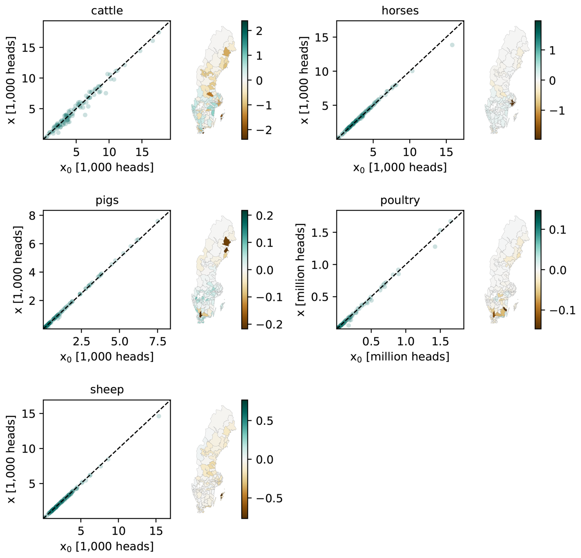
Figure 4 Regional distribution of animals in CIBUSmod (x) compared to animal numbers estimated from national statistics (x₀). The dashed lines shows the 1:1 lines. The maps show x – x₀ per region. Animal numbers are expressed in terms of the number of the defining animal category per species (cows for cattle, ewes for sheep, total horses, sows + gilts for pigs and broilers or laying hens for poultry).

In Sweden, statistics on animal feeding practices are not routinely collected, which makes it difficult to validate assumptions about feed rations. The feed industry do however report data on the raw materials used in compound feeds. Many crop products and some by-products used in animal feed bypass the feed industry and are thus not represented in these statistics. For by-products that are primarily supplied through compound feeds, some validation was possible using national statistics, as shown in Fig. 6. This comparison generally shows reasonable alignment, although the assumed feed rations here lead to an overestimation of soybean meal use and an underestimation of rapeseed meal use compared to the feed industry statistics. This discrepancy is likely due to recent efforts in Sweden to reduce soybean meal in animal feed, given its association with deforestation in South America – a shift that was not reflected in the data used to estimate feed rations.

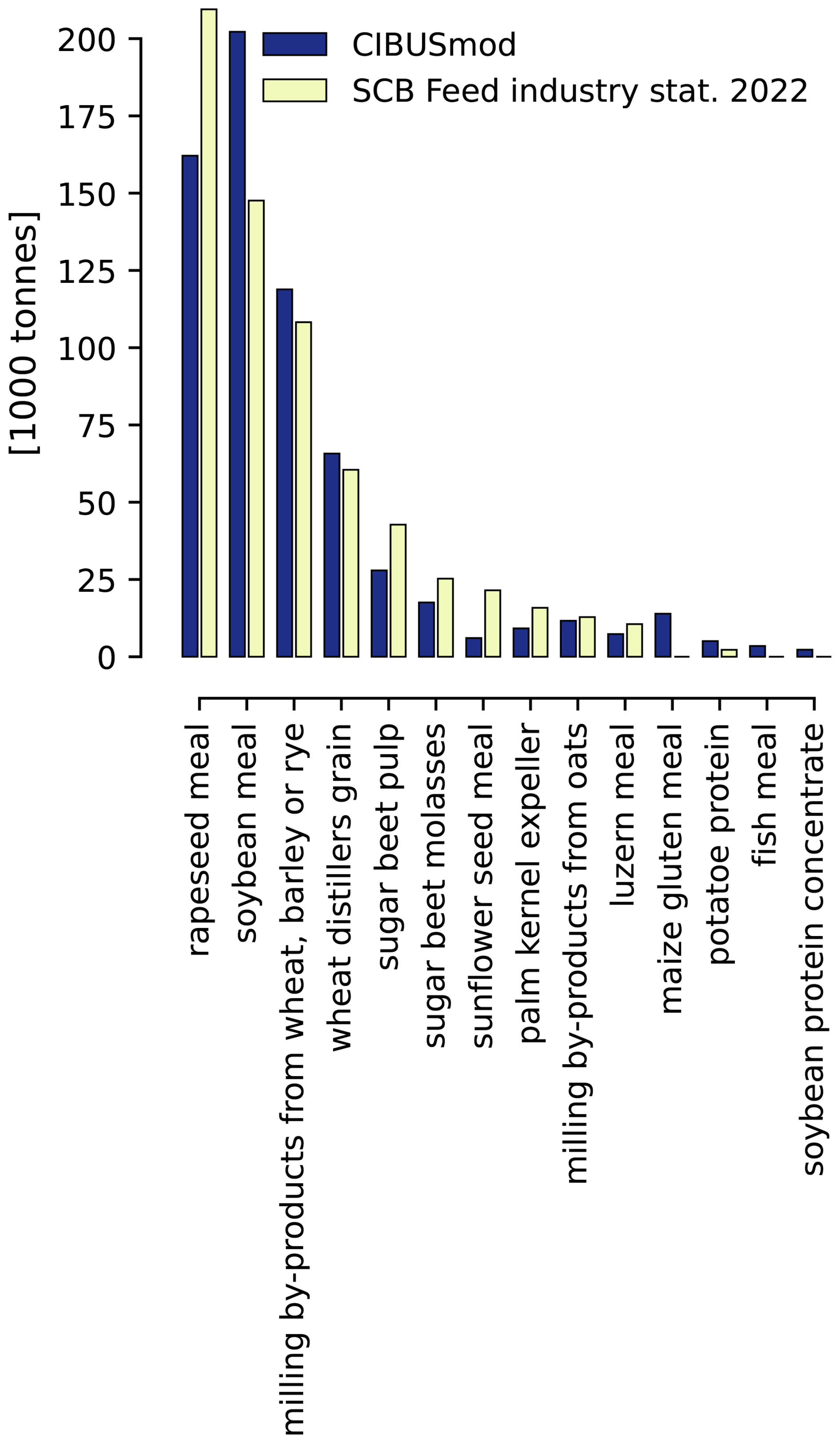
Figure 5 Use of by-products in animal feed estimated in CIBUSmod compared to national feed industry statistics for year 2022.

3.1.4 Fertiliser and manure

Parameters used to estimate crop N, P and K requirements were sourced mainly from national fertiliser recommendations from the Swedish Board of Agriculture (2023), using region- and soil class-specific recommendations when available. For crops not covered by national recommendations (e.g. vegetables, barriers and fruit), recommendations from fertiliser manufacturers or values from previous studies were used.

Data used to estimate manure N, P and K excretion for cattle and pigs under the mass-balance approach was based on Dutch data (Statistics Netherlands, 2012). For other livestock categories excretion rates per head were sourced from (Swedish Environmental Protection Agency, 2023b) for N and from Statistics Netherlands (2012) for P and K. Emission factors used in estimating N losses in stables and manure storage were sourced from the (Swedish Environmental Protection Agency, 2023a) and the European Environment Agency (2023).

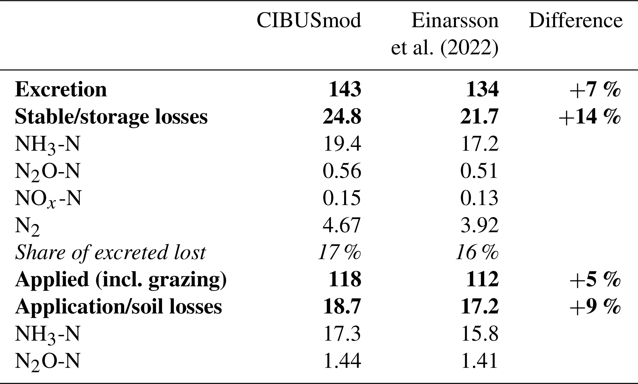
The total N excretion in manure is estimated at 143 000 t in CIBUSmod, with 17 % lost during storage and in stables (Table 3). This total excretion is 7 % higher than the estimates by Einarsson et al. (2022), resulting in proportionally larger losses estimated in CIBUSmod. The discrepancy is due to differences in methodology: Einarsson et al. (2022) estimated manure excretion using fixed factors per animal, whereas a mass-balance approach is used in CIBUSmod for cattle and pigs. However, estimates from CIBUSmod are well in line with national statistics on to total manure application on cropland for both N and P (Fig. 6). Considering the complexity and uncertainties, the mass-balance approach for calculating N, P, and K excretion yields estimates within an acceptable range of other estimates. Unlike fixed excretion rates per animal, this approach offers the advantage of internally calculating excretion rates based on animal productivity, the feed requirements and its composition.

Table 3 Estimated nitrogen (N) in excreted manure and losses in stables and during manure storage in CIBUSmod compared to estimates reported in Einarsson et al. (2022). Values are given in 1000 t N, with bold font used for aggregated figures and italics for the percentage of excretion lost in stables and during storage.

Total mineral N fertiliser application on cropland in CIBUSmod is estimated at 145 000 t, which is 15 % lower than the figure reported in national statistics (Fig. 6). This discrepancy is due to an underestimation of total crop areas in the model compared to national statistics data. When crop areas from national statistics were used directly in the model, estimated mineral N fertiliser application was 1 % higher than reported in national statistics.

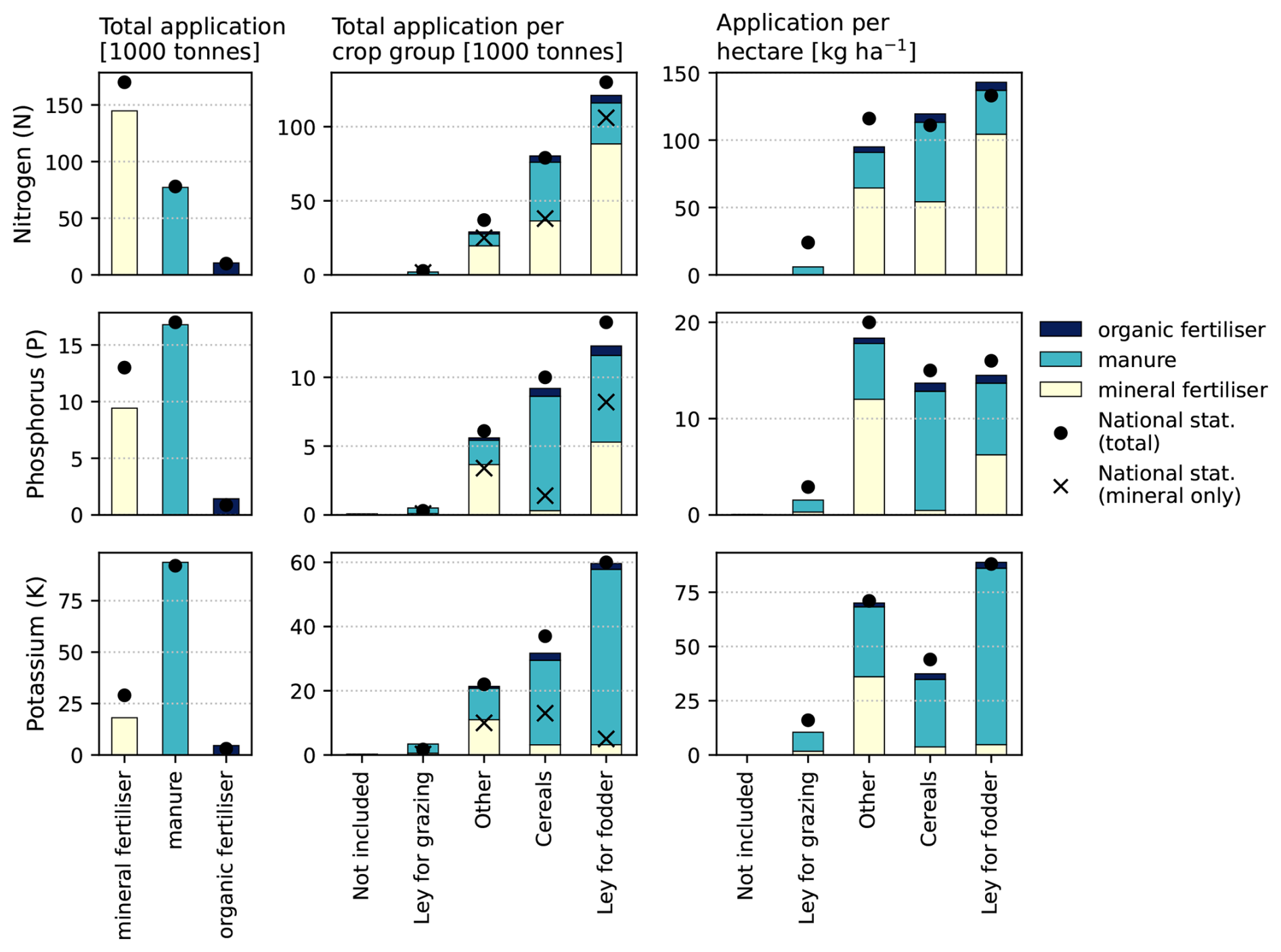
Figure 6 Nitrogen (N), phosphorus (P) and potassium (K) application on cropland in CBUSmod compared to national fertiliser statistics (average 2016–2020). Bars show results from CIBUSmod and points and crosses show total and mineral fertiliser application according to national statistics, respectively.

The regional distribution of N application in mineral fertilisers and manure estimated in CIBUSmod follows the general patterns observed in national statistics (Fig. 7). But, application rates of mineral fertiliser in the forest-dominated south-central and northern parts of Sweden are lower in CIBUSmod compared to national statistics.

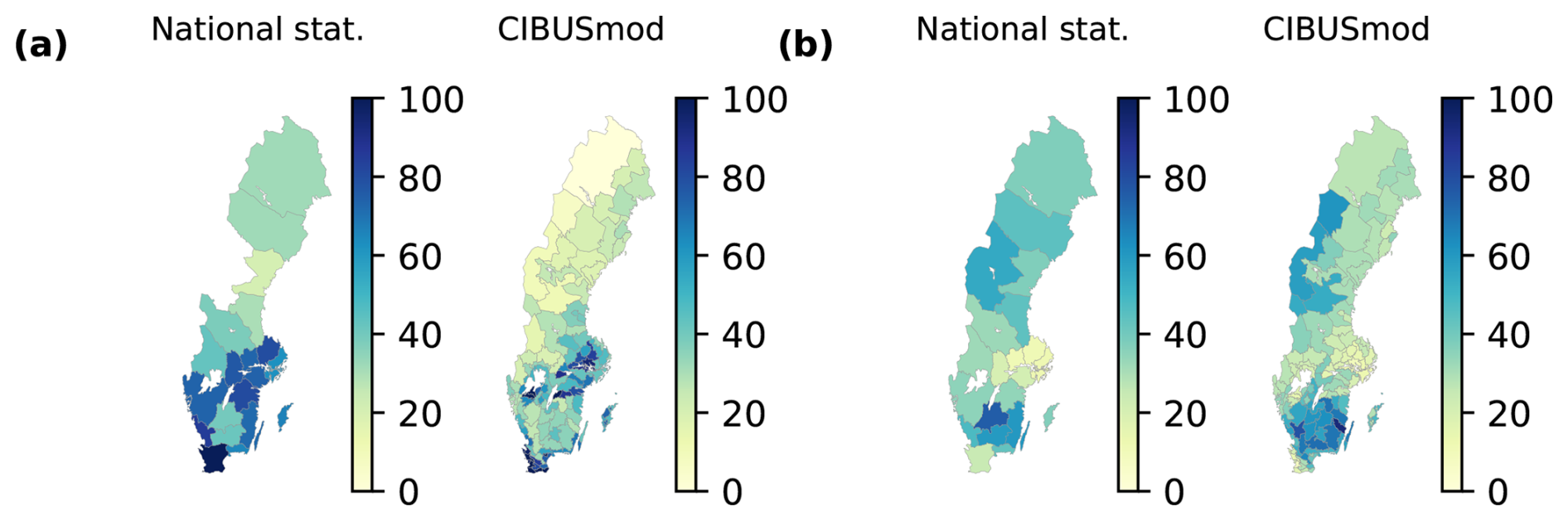
Figure 7 Geographic distribution of mineral fertiliser (a) and manure (b) nitrogen application on croplands according to national fertiliser statistics and in CIBUSmod expressed as kg N ha⁻¹.

3.1.5 Energy use

Data for the parameters used in estimating energy use for field machinery, grain dryers, animal stables and greenhouses were compiled from a number of sources, comprising mainly of Swedish technical reports, including an inventory of energy use in Swedish agriculture commissioned by the Swedish Board of Agriculture and summarised in Baky et al. (2010). For the main tractor implements, soil-type-specific parameters were sourced from ASABE (2006). Figure 8 shows that estimated energy use in CIBUSmod aligns well with those previously presented by Baky et al. (2010), albeit with some exceptions, notably for pig and broiler stables where substantially lower energy use was estimated using CIBUSmod.

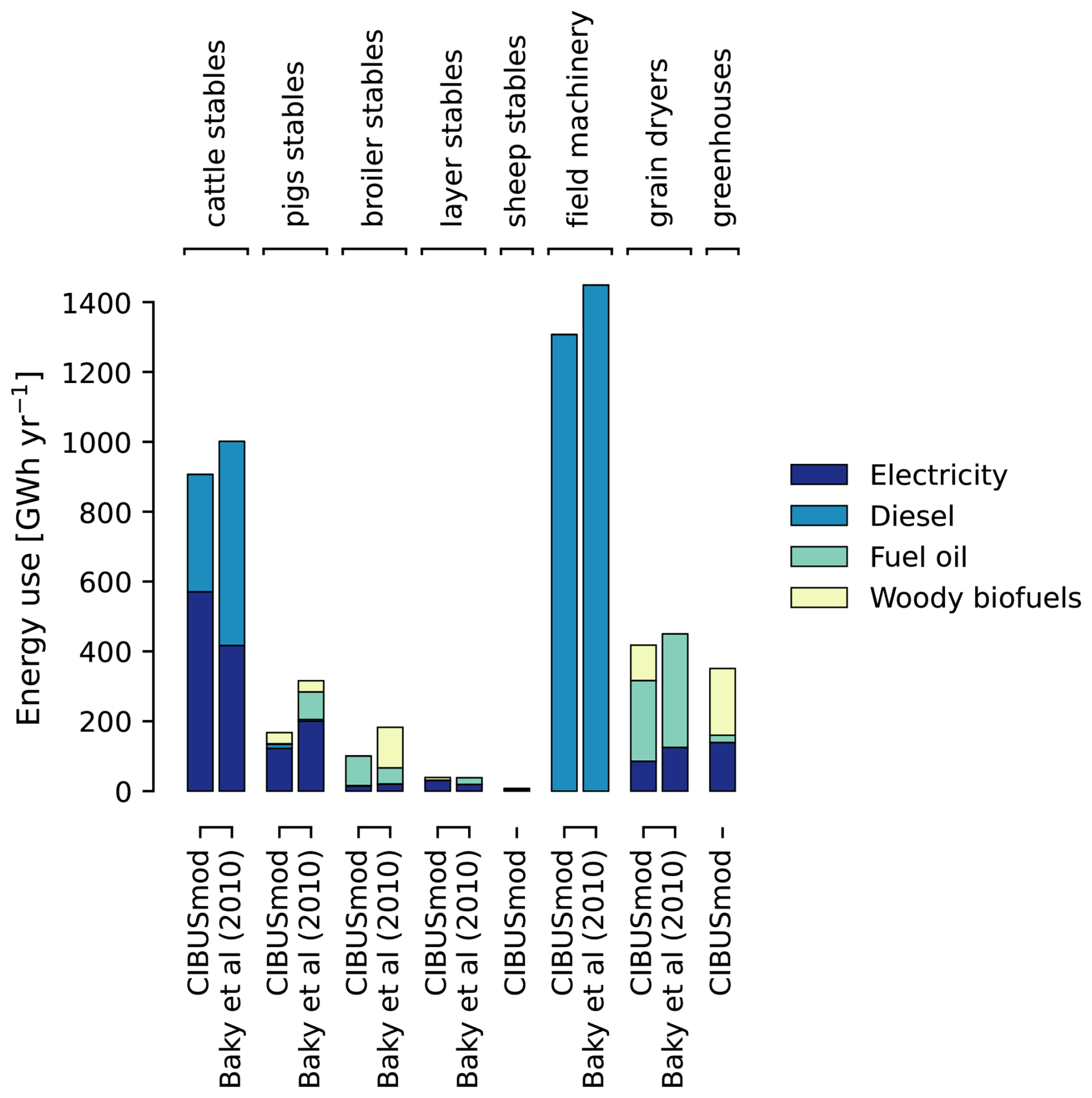
Figure 8 Energy use in stables, field machinery, grain dryers and greenhouses subdivided by energy source estimated in CIBUSmod compared to estimates by Baky et al. (2010).

3.1.6 Greenhouse gas emissions

Figure 9 compares methane and nitrous oxide emissions from Sweden's national greenhouse gas inventory with those estimated by CIBUSmod, which shows that emissions estimated in CIBUSmod largely are in agreement with values in the national inventory. For methane, the results show good agreement for enteric fermentation (Fig. 9, 3.A). However, for manure management (Fig. 9, 3.B(a)), CIBUSmod estimates significantly higher emissions for horses and poultry. The national inventory uses fixed emission factors per head from IPCC (2006) for these livestock categories, while CIBUSmod bases emissions on volatile solids (VS) excretion, which in turn is derived from gross and digestible energy in feed rations (see Sect. 2.5) for all livestock. Default VS excretion for poultry are given as 0.010 kg VS per animal and day for broilers and 0.020 kg VS per animal and day for laying hens with a margin of error of ± 50 % in IPCC (2006). In contrast, the estimates from CIBUSmod, based on feed consumption, are twice as high for broilers (0.020 kg VS) while for laying hens estimates align more (0.022–0.024 kg VS). Moreover, the methane emission factors used in the national inventory are based on only dry manure management systems for laying hens. In the case study it is assumed that 8 % of laying hens have a liquid manure management system, in accordance with the Swedish Environmental Protection Agency (2023a), which has more than an order of magnitude higher MCF factor than dry systems (IPCC, 2019). Together, these methodological differences explain the large discrepancies in emission estimates.

For nitrous oxide emissions from manure management (Fig. 9, 3.B(b)), the results are more consistent between the two sources, but CIBUSmod estimates higher emissions, particularly for cattle and pigs. The mass balance approach used in CIBUSmod to estimate N excretion (see Sect. 2.5.1) result in higher excretion rates than the figures used in the national inventory, which explains the difference.

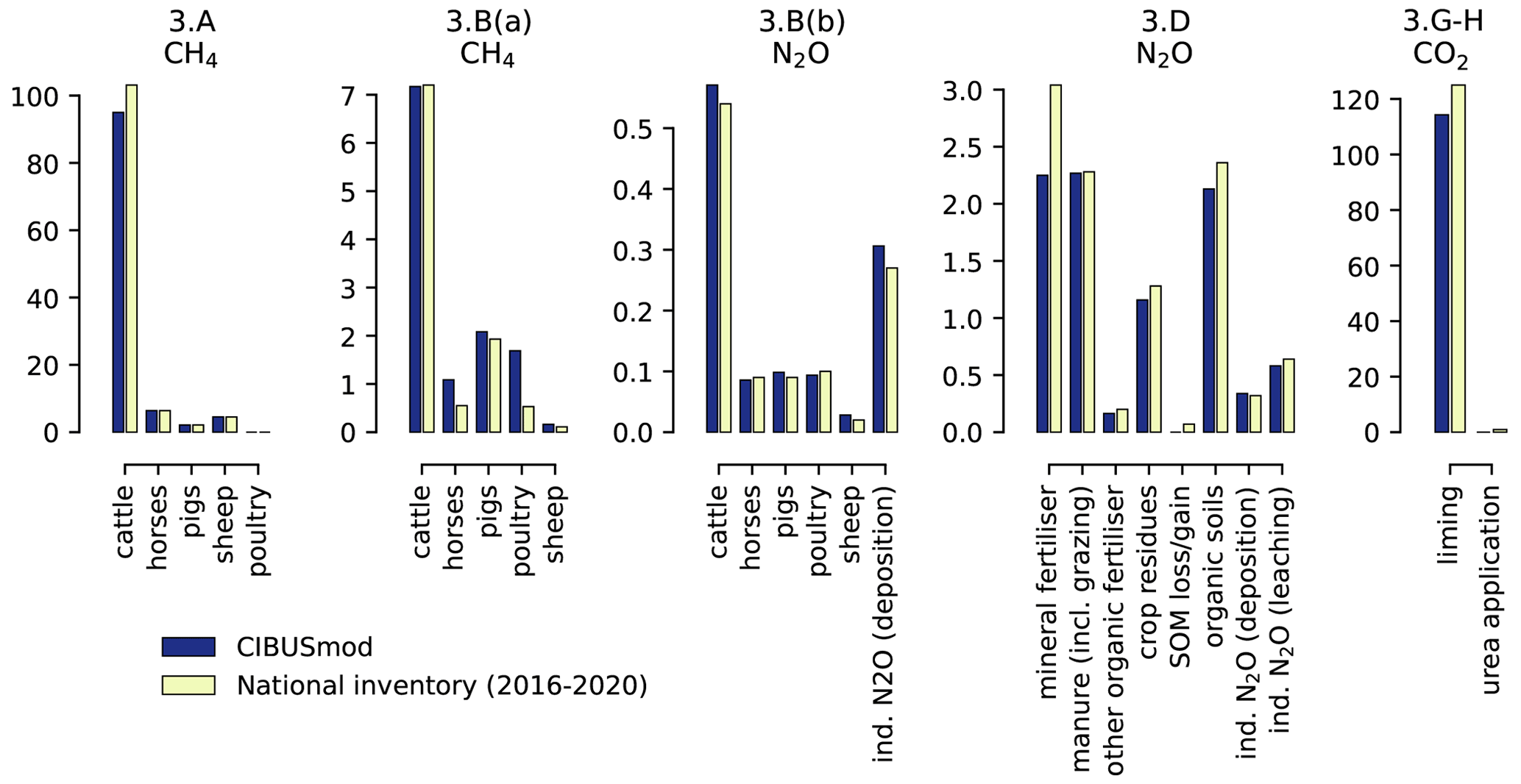
Figure 9 Agriculture sector emissions in 1000 t of carbon dioxide (CO₂), methane (CH₄) or nitrous oxide (N₂O) as reported in Sweden's National Inventory Report (NIR) to the United Nations Framework Convention on Climate Change (average for 2016–2020) compared to corresponding emissions estimated in CIBUSmod. The labels correspond to the common reporting format (CRF) table numbers: 3.A = Enteric Fermentation, 3.B(a) = CH₄ Emissions from Manure Management, 3.B(b) = N₂O Emissions from Manure Management, 3.D = Direct and indirect N₂O emissions from agricultural soils, 3.G-H = CO₂ emissions from liming, urea application and other carbon-containing fertilizers.

Regarding nitrous oxide emissions from agricultural soils (Fig. 9, 3.D), CIBUSmod estimates lower emissions from mineral fertiliser application due to the underestimation of fertiliser use, as discussed earlier, while for manure estimates agree with the national inventory. Moreover, emissions from crop residues are estimated slightly lower in CIBUSmod compared to the national greenhouse gas inventory. This is partly explained by a larger share of crop residues being removed in the CIBUSmod. In CIBUSmod the fraction of crop residues removed is endogenously calculated based on demand for bedding material in stables. This may indicate that parameters used for estimating the use of bedding materials overestimate total demand or that use of straw is underestimated in the national inventory. Estimated indirect nitrous oxide emissions from deposition and leaching are comparable to what is reported in the national inventory. While the national inventory, uses a sophisticated process-based model to estimate leaching, CIBUSmod estimates leaching as a fixed share of N inputs, according to IPCC (2019) Tier 1 methodology. A leaching factor of 0.144 kg N leached per kg N input, developed for Finland's national inventory report, was used across all crops.

For nitrous oxide emissions from managed organic soils slightly lower emissions were estimated in CIBUSmod than reported in the national inventory. This is a net effect of the total area of cropland on organic soils being lower in CIBUSmod than in the national inventory (mainly due to a lower total cropland use) and that emissions from semi-natural grasslands on organic soils are included in CIBUSmod, which are reported under forestry in the national inventory. Data on the share of cropland and semi-natural grasslands on peat soils from Lindahl and Lundblad (2021) was used to estimate the area of organic soils.

Carbon dioxide emissions associated with liming are slightly lower in CIBUSmod than in the national inventory (Fig. 9, 3.G-H) due to CIBUSmod estimating a lower total use of lime. Emissions from urea are not estimated in CIBUSmod, but these emissions are negligible in Sweden.

3.2 Scenario example – Re-assessing scenarios for organic farming in Sweden

In this section, an example of model runs comparing two scenarios is presented to illustrate the model's behaviour and its outputs. Both scenarios were modelled from 2020 to 2050, using 2020 as the baseline year. The scenarios were based on the “Base20” and “Sust50” scenarios for Sweden, originally developed by Basnet et al. (2023). In Basnet et al. (2023) these scenarios were modelled using the FABLE Calculator (Mosnier et al., 2020).

The Base20 scenario represents a business-as-usual pathway. It incorporates crop and livestock productivity improvements, as well as population growth. In contrast, Sust50 envisions a shift to organic farming covering approximately 50 % of Swedish cropland by the year 2050 (implemented in CIBUSmod by increasing organic food consumption). In this scenario diets change to include fewer animal-source foods and more vegetables and fruits, household food waste is reduced by 50 %, and productivity improvements are stronger than in Base20. Import shares are held constant for all foods in both Base20 and Sust50, but the Sust50 scenario includes increased organic cereal exports. Further details on scenario definitions can be found in Basnet et al. (2023).

In addition to the definitions provided by Basnet et al. (2023), several adjustments were made to the Sust50 scenario to ensure adequate nutrient supply in organic cropping systems. Specifically, the area dedicated to green manure in organic systems was increased by enforcing at least 10 % of organic cropland devoted to green manures. The maximum share of cereals in organic crop rotations was also constrained (8 % and 15 % for winter and spring cereals, respectively) to limit regional nutrient requirements. The proportion of food waste directed to anaerobic digestion was increased, from 40 % in 2020 to 80 % for household food waste and 100 % for processing and retail food waste. Grass-legume ley cultivation was also introduced as feedstock for anaerobic digestion in order to increase nutrient supply in the form of digestate as an organic fertiliser. In both scenarios, total cropland increase was constrained not to increase by more than 20 % from baseline levels in any region.

3.2.1 Scenario example results

Consistent with Basnet et al. (2023), the cropland areas from CIBUSmod remain stable in the Base20 scenario, as productivity improvements meet the rising demand driven by population growth (Fig. 10). However, while Basnet et al. (2023) report a reduction in cropland use under the Sust50 scenario, the results from CIBUSmod indicate unchanged cropland use in 2050 compared to 2020. A major reason for this discrepancy is the assumed increase in green manure in CIBUSmod, where this area increases from less than 1 % of organic cropland in 2020 to 10 % in 2050 (Fig. 12b). This contributes to adequate N supply for organic crop production.

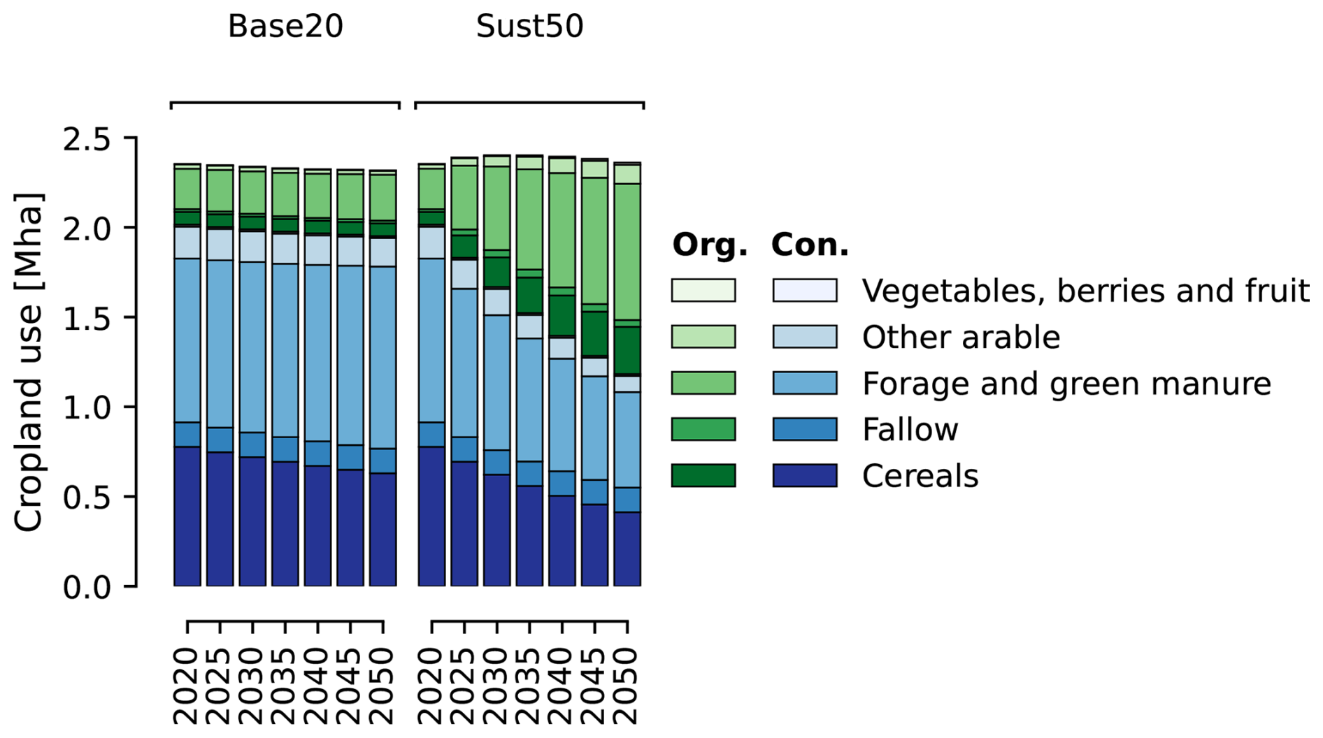
Figure 10 Development of cropland use for the two scenarios. Blue and green shades show conventional and organic areas respectively.

In the base year, 56 kg N ha⁻¹ was applied to organic cropland (Fig. 11a) through animal manure and other organic fertilisers (i.e. biogas digestate from anaerobic treatment of waste and manure). Approximately 24 % of N input to organic farming originated from conventional animal manure. This flow of nutrients from conventional agriculture underscores the dependence of current organic production systems on conventional nutrient sources, as highlighted by e.g. Nowak et al. (2013) and Vergely et al. (2024). Under the Sust50 scenario, N application to organic cropland increased to 62 kg N ha⁻¹, despite the increase in green manures, due to an increased share of organic cropland devoted to cereals. In CIBUSmod, N fixation from green manure and other leguminous crops is not directly visible in outputs. It is instead accounted for indirectly through crop-specific parameters for residual N which becomes available to subsequent crops in the rotation. This effectively reduces N requirements. The increased N fixation in green manures, along with increased digestate supply from anaerobic digestion of food waste and ley biomass (Fig. 12a) reduced the reliance on conventional animal manure for organic production to 14 % of total N inputs in the Sust50 scenario (Fig. 11b).

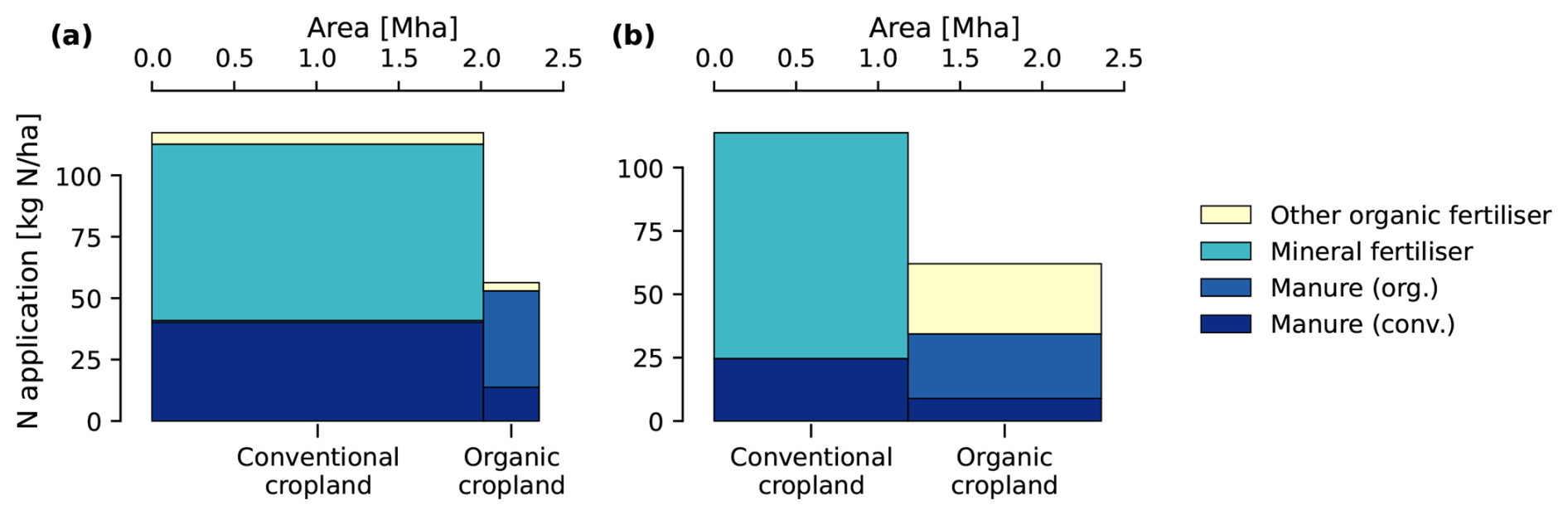
Figure 11 Distribution of nitrogen (N) in mineral fertilisers, manure and other organic fertilisers (i.e. biogas digestate) to conventional and organic cropland in the base year 2020 (a) and in 2050 for the Sust50 scenario (b). The x-axis shows the total cropland area and the y-axis N application per hectare. The area of each box is thus proportional to total N application.

In the Base20 scenario, animal manure N application increased, while reduced animal-source food consumption in the Sust50 scenario led to reduced livestock populations and manure supply (Fig. 12d). In the Base20 scenario, mineral N fertiliser use reduced slightly while the Sust50 scenario led to a substantial reduction in fertiliser use, from around 145 kt N in the base year to 106 kt N in 2050 (Fig. 12c).

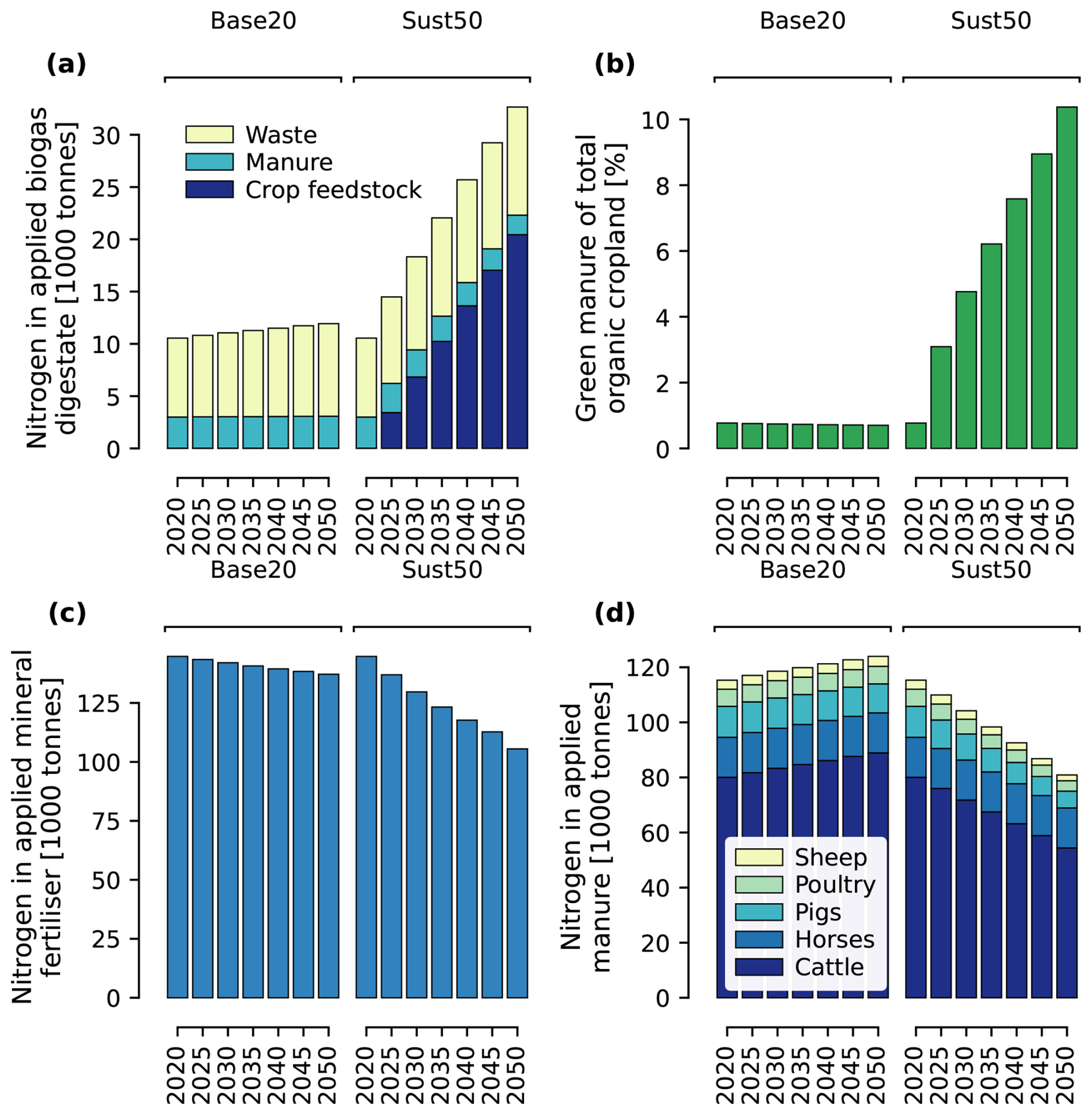
Figure 12 Development of key variables for nitrogen supply for the two scenarios. (a) Nitrogen in applied digestate per feedstock type, (b) share of total organic cropland devoted to green manure, (c) applied mineral fertilisers and (d) applied animal manure per livestock species.

In the Base20 scenario, GHG emissions from the agricultural sector (including energy use and input supply chain emissions) increased, whereas in the Sust50 scenario, emissions of CO₂, CH₄, and N₂O were reduced by 7 %, 24 % and 15 %, respectively, by 2050 (Fig. 13). The total climate impacts in CO₂-equivalent terms were reduced by 15 %. This was largely due to decreased livestock numbers and mineral N fertiliser use. In the original scenario assessment by Basnet et al. (2023), production emissions in CO₂-equivalent terms were projected to decrease by approximately 38 % from 2010 to 2050 under the Sust50 scenario. Additionally, a net carbon sequestration opportunity due to reduced cropland requirements was identified. In contrast, results from CIBUSmod indicates unchanged cropland use, and thus no opportunities for increasing carbon sequestration through afforestation. Consequently, the results from CIBUSmod suggests that while the Sust50 scenario has substantial emissions reduction potential, it is lower than estimated in Basnet et al. (2023).

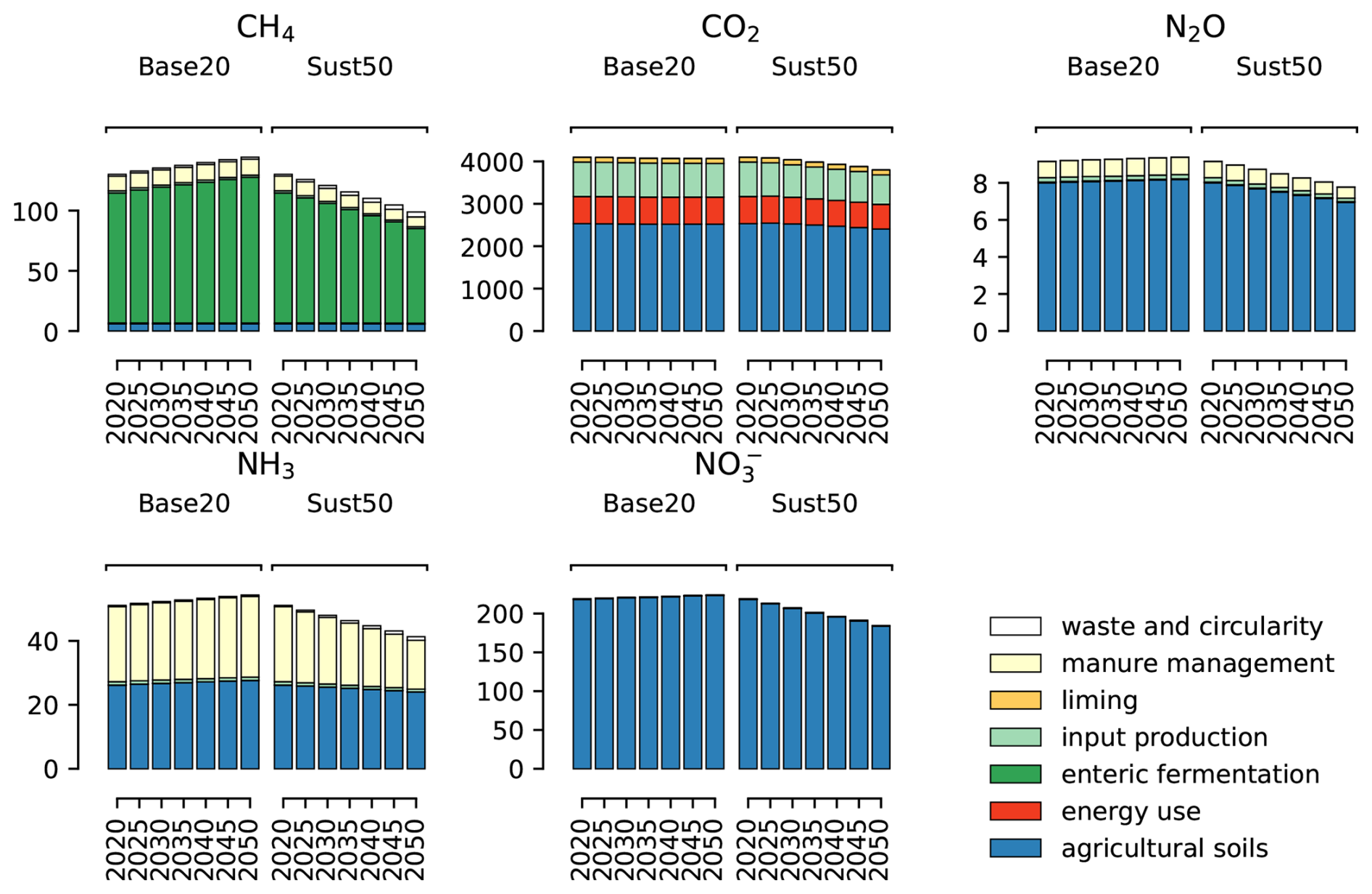
Figure 13 Development of yearly emissions [1000 t] of methane (CH₄), carbon dioxide (CO₂), nitrous oxide (N₂O), ammonia (NH₃) and leaching of nitrate (NO${}_{\mathrm{3}}^{-}$) under the Base20 and Sust50 scenarios.

The share of cropland under organic farming ranged from 17 %–68 % across regions. It followed approximately the initial distribution of organic cropland areas (Fig. 14a), which is expected as deviations from the initial state are minimised in the model. The assessment of regional N budgets showed that biogas digestate would need to be moved from regions with surplus to those with a deficit to meet local crop nutrient requirements. In the Sust50 scenario, it was assumed that biogas digestate would be prioritised for organic areas to reduce reliance on conventional animal manure in organic farming. This would pose major logistical challenges. Increasing the use of conventional animal manure on organic cropland or directing animal farming and ley production for anaerobic digestion to more productive regions with high crop N requirements, could potentially reduce the need for transport of N between regions. This was however not investigated further in this study.

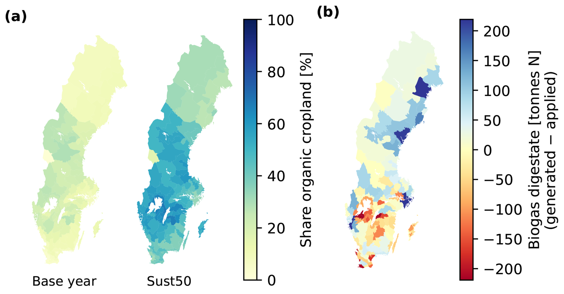
Figure 14 (a) Share of cropland under organic production in the base year (2020) and in 2050 under the Sust50 scenario. (b) Difference between generated and applied biogas digestate in terms of nitrogen (N) in the Sust50 scenario in 2050.

In summary, the results from the CIBUSmod modelling framework underscore the importance of considering nutrient flows in the agri-food system when evaluating scenarios for large-scale expansion of organic production. This aspect was not covered in the original analysis by Basnet et al. (2023), explaining the differences in results regarding land requirements and, consequently, in opportunities for carbon sequestration on “spared” cropland. It should however be noted that there are many options for enhanced nutrient supply in organic farming systems with limited land requirements that were not explored in this study. Such strategies could include increased recirculation of human excreta (Harder et al., 2019), introducing leguminous cover crops (Tribouillois et al., 2016) or harvesting nutrients from the sea (Spångberg et al., 2013). Furthermore, the Sust50 scenario was defined in CIBUSmod with an aim to reduce reliance on conventional animal manure in organic production. Allowing more conventional animal manure on organic cropland would reduce the need for green manures. But it would also increase mineral N fertiliser requirements, as animal manure would be redirected from conventional to organic cropland.

4 Discussion and conclusions

This paper presents a proof of concept for the CIBUSmod modelling framework. It demonstrates how input data can be collected and validated to establish a baseline. From this, scenarios involving different demand- and supply-side interventions can be developed and assessed.

While several similar models exist (e.g. Müller et al., 2020; Kalt et al., 2021; Jones et al., 2023; van Zanten et al., 2023), CIBUSmod offers key features that distinguish it from previous frameworks. Notably, it is open-source and provides a high degree of flexibility, allowing users to parametrise any number of regions, food items, crops, and livestock production systems. It also includes a detailed account of nutrient flows, as well as waste and food processing by-products, along with their end-use application in animal feed or energy/nutrient recovery.

Although CIBUSmod is designed for modelling story-driven scenarios, it is relatively lightweight, enabling the exploration of “option spaces” that incorporate numerous scenarios with varying assumptions on key parameters such as crop yields, diets, and waste levels. This aligns with approaches used by Muller et al. (2017) and Kalt et al. (2021). This scenario development method has already been applied with CIBUSmod to assess the effects of reduced red meat intake recommendations in Sweden on land use, greenhouse gas emissions, and ammonia emissions (Slijper et al., 2024; Karlsson Potter et al., 2025). Additionally, CIBUSmod allows for the decomposition of scenarios into their principal components, applying sets of parameter changes in sequence. This facilitates an analysis of the relative importance of different supply- and demand-side interventions within a given scenario.

Because of its relatively high level of detail, CIBUSmod is primarily designed to be used with direct involvement of researchers. However, the ambition is for it to be a valuable resource also in education and collaborative foresight projects where alternative future scenarios are jointly developed and explored. This can be done, for example, through an iterative story-and-simulation process (Volkery et al., 2008; Karlsson et al., 2018), where stakeholders draft scenario narratives that researchers translate into quantitative model inputs. Alternatively, simplified Excel workbooks that contain a limited set of adjustable parameters, along with explanations of what each parameter represents, can be constructed. This enables participants to directly modify inputs and test different scenarios without the need for a comprehensive understanding of the model in its entirety. This latter approach has already been applied in PhD-level education, where student teams created narratives of future food systems and translated them into quantitative parameter changes. The model was then run, and results analysed to see whether outcomes matched expectations. Students were then able to investigate which levers had the strongest effect on key outcome variables as well as cases where their prior assumptions diverged from the model's behaviour.

Future work will build on this foundation, expanding the modelling framework as new research questions emerge. However, several known limitations and planned model developments already exist, as outlined in the following sections.

At present, land use and emissions are calculated only for domestic production, up to farm gate, including the supply chains for fertiliser and energy inputs. The model does not yet account for impacts arising from food processing and distribution. It also does not include impacts generated abroad, either directly through food and feed imports, or indirectly through exports. Import and export quantities are currently generated as outputs, and future development will focus on linking these to datasets that combine trade data with environmental impacts for traded food and feed commodities, such as the one developed for the SAFAD tool (Röös et al., 2025), to quantify associated impacts. Alternatively, CIBUSmod outputs could be integrated with global-scale modelling frameworks, such as the one used by Mosnier et al. (2023).

For food processing, CIBUSmod accounts for material flows, including losses and generated by-products, but does not yet consider energy use in transports and processing beyond the farm gate. This omission can have significant impact when assessing scenarios that include a high proportion of novel or highly processed foods, such as meat analogues, where a large share of environmental impacts are associated with energy use in processing (Mejia et al., 2020). Additionally, modelling scenarios that alter food processing – and therefore the quantity and quality of by-products, often used for animal feed – poses challenges in the current version. Currently, animal diets are input manually and any mismatch in supply and demand for by-products is corrected by adjusting imports and exports, or waste. To avoid this, feed rations would need to be manually refined to align with by-product supply in different scenarios, which is a tedious process often not practically feasible. In addition, the current approach requires the user to supply balanced feed rations for the different animal categories with regards to e.g. protein-to-energy ratio and energy density, which requires animal nutrition competence to ensure nutritionally adequate feed rations. However, Wanecek (2025) presents an extension of CIBUSmod that incorporates feed rations into the optimisation problem, allowing them to be determined endogenously based on available feedstuffs and livestock nutritional requirements. This development will enable feed rations to respond dynamically to changes in by-product availability and composition under different scenarios, facilitating research on e.g. optimised use of local resources for animal feed.

In its current version, CIBUSmod models nutrient leaching from agricultural land only in terms of N leaching, using a basic method that does not directly account for management practices that reduce leaching. Future work will aim to incorporate improved methods to estimate both N and P leaching and runoff, incorporating regional differences in soil and climate while accounting for different management practices.

Changes in carbon stocks due to land use and land-use change are currently only modelled for organic soils, using emission factors for CO₂ and CH₄ ha⁻¹. The version of the model presented here does not include changes in carbon stocks resulting from shifts in agricultural land use or mineral soil organic carbon dynamics. A module that models changes in mineral soil carbon stocks, based on carbon inputs from crop residues, manure, and other organic sources, using the ICBM model (Andrén et al., 2004) is however being developed and will be incorporated in future versions. Future work will also include modelling changes in soil and standing biomass carbon pools due to land use changes (i.e. expansion or retraction of agricultural land use).

At present, the model includes impact assessment methods for climate impacts, allowing users to select different approaches such as GWP, GTP, or time-dynamic climate impacts. Output also include land use and nutrient flows which readily allow the calculation of additional indicators for environmental impacts, such as “new N and P inputs” (Ran et al., 2024) or the application of methods to characterise biodiversity impacts from land use (e.g. Chaudhary and Brooks, 2018). However, the capacity to identify trade-offs across multiple environmental and social sustainability dimensions is still limited. Future development will expand the framework by incorporating additional impact categories and inventory models, including eutrophication, biodiversity impacts, animal welfare, and nutritional indices for diets.

It is important to note that CIBUSmod is a strictly biophysical mass-flow model. It cannot assess the policies or other socio-economic conditions required to realise a given scenario, nor the socio-economic impacts of that scenario. However, biophysical food system models have previously been combined with economic models to analyse the policies needed to achieve specific outcomes (Röös et al., 2022) – an approach that could also be applied with CIBUSmod.

To conclude, CIBUSmod provides an open-source, modular and spatially explicit framework for assessing national agri-food system scenarios supporting detailed analyses of land use, nutrient flows and emissions. The Swedish case study illustrates the model's capacity to reproduce baseline patterns and evaluate alternative scenarios. As such, CIBUSmod can hopefully offer a practical and adaptable platform for researchers engaged in food systems sustainability analysis.