Subgrid corrections for the linear inertial equations of a compound flood model – a case study using SFINCS 2.1.1 Dollerup release

Accurate flood risk assessments and early warning systems are needed to protect and prepare people in coastal areas from storms. In order to provide this information efficiently and on time, computational costs in flood models need to be kept as low as possible. One way to achieve this goal is to apply subgrid corrections to relatively coarse computational grids. Previously, these have been used in full-physics circulation models. In this paper, for the first time, we developed subgrid corrections for the linear inertial equations (LIEs) that account for bed level and friction variations. They were implemented in the Super-Fast INundation of CoastS (SFINCS) model version 2.1.1 Dollerup release. Pre-processed lookup tables that correlate water levels with hydrodynamic quantities make more precise simulations with lower computational costs possible. These subgrid corrections have undergone validation through several conceptual and real-world application scenarios, including rainfall-induced flooding during a hurricane and tidal propagation in an estuary. We demonstrate that the subgrid corrections for linear inertial equations significantly improve model accuracy while utilizing the same resolution without subgrid corrections. In terms of computational efficiency, subgrid corrections increase computational costs by 38 %–128 %. However, this yields a 35–50-time speedup since coarser model resolutions with subgrid corrections can provide the same accuracy as finer resolutions without subgrid corrections. Limitations are also discussed; for example, when grids do not adequately resolve river meanders, fluxes can be overestimated. Our findings show that subgrid corrections are a useful asset for hydrodynamic modelers striving to achieve a balance between accuracy and efficiency.

1 Introduction

With hundreds of millions of people living in areas with an elevation of less than 10 m above sea level (McGranahan et al., 2007), coastal zone flooding has large consequences for casualties and damage to real estate and infrastructure. To protect and mitigate flood damages and loss of life, a priori risk assessments may inform decision-makers in what locations and under what circumstances flooding occurs and what interventions to take. Both risk assessments and early warning systems should provide information that is as accurate as possible so as not to give false warnings or needlessly over- or underestimate the extent and cost of interventions.

For flood warnings, this means that simple bathtub approaches, where a peak water level is imposed on an area's topography, do not suffice. They may overestimate the flood intensity because the surge hydrograph is not taken into account (Vousdoukas et al., 2016) or underestimate it due to lacking physics (e.g., wave effects, Didier et al., 2020) or lacking inputs such as roughness effects which would impede flow (Ramirez et al., 2016). Therefore, for a more accurate flood estimate, the dynamic aspects of floods, such as the duration of an event and the path that flood waters take, should be considered. Furthermore, the compound nature of coastal area floods, which may be caused by a combination of marine surges, wave overtopping, coastal river discharges, and local rainfall needs to be taken into account. These dynamics and processes may be resolved using process-based numerical models which are based on the conservation of mass and momentum. While classical full-complexity models (ADCIRC, Luettich et al., 1992; Delft3D-FLOW, Lesser et al., 2004; MIKE, Warren and Bach, 1992; or SOBEK, Stelling et al., 1998) offer highly detailed simulations, they often require substantial computational resources, particularly for high-resolution simulations over large areas or when exploring uncertainties in flooding through ensemble modeling. Although these models can be applied to large-scale systems with adequate computing power, their high computational demands may constrain their practical use in time-sensitive or resource-limited scenarios.

To that end, reduced-complexity models have been developed and applied in riverine and coastal settings. Examples include, among others, the LISFLOOD-FP model by Bates et al. (2010) and the SFINCS (Super-Fast INundation of CoastS) model by Leijnse et al. (2021). These models focus on solving reduced forms of the momentum equations using a simplified numerical scheme, allowing them to run significantly faster than traditional full-complexity models. Still, the number of simulations that can be run is limited as the numerical scheme is explicit and therefore strongly influenced by the spatial grid size (and associated time step).

One way to further increase computational speed is to apply a subgrid approach which makes use of the assumption that water level gradients are typically much smaller than topographic gradients. Defina (2000) presented shallow-water equations with mass conservation corrections to account for wetting and drying areas and corrections to the momentum equations to account for varying velocities. Casulli (2009a) introduced a dual-grid approach with a higher-resolution grid for the bathymetry and a lower-resolution grid for the hydrodynamics, where the depth and cross-sectional area were computed using the higher-resolution grid and stored in lookup tables which were used to evaluate the water levels on the lower-resolution grid. Volp et al. (2013) extended Casulli's approach to finite volumes and incorporated subgrid corrections to compute advection and bottom friction under the assumptions of locally uniform flow direction and friction slope. Sehili et al. (2014) showed that subgrid corrections could save an order of magnitude of computational cost without major accuracy loss in estuarine modeling. For coastal storm surge applications, Kennedy et al. (2019) developed a refined set of equations incorporating extra terms derived from an upscaling technique. These additional terms, emerging from the averaging of shallow-water equations, account for the integral properties of fine-scale bathymetry, topography, and flow dynamics. This process is similar to how Boussinesq approximations are used for turbulence closure in Navier–Stokes models and involves using coarse-scale variables, such as averaged fluid velocity, to represent these fine-scale integrals. They showed the improved performance of their model for the case of tidal flooding in a small bay. Woodruff et al. (2021) extended this analysis to a case of storm surge with realistic atmospheric forcing and reported a speedup of ADCIRC by a factor of 10–50. Similarly, Begmohammadi et al. (2023) adapted the numerical implementation of the real-time forecasting model SLOSH (Jelesnianski et al., 1992) to improve inundation performance in a coastal region with narrow channels. Woodruff et al. (2023) scaled up these approaches to the entire South Atlantic Bight and showed improved performance of a subgrid model compared to a conventional high-resolution model for Hurricane Matthew (2016).

More recently, subgrid models such as CoaSToRM (Begmohammadi et al., 2024) and HEC-RAS (Brunner, 2016) have further advanced the field. CoaSToRM is a standalone solver for compound flooding in coastal regions, utilizing subgrid topography to improve inundation accuracy in overland and coastal flood modeling. HEC-RAS nowadays also allows for the integration of subgrid corrections, utilizing detailed hydraulic property tables to improve performance in both riverine and coastal flood scenarios.

While these advances have led to great improvements in estuarine and storm surge modeling, the assumption of hydraulic connectivity of subgrid cells remains a challenge. To that end, Casulli (2009b) and Begmohammadi et al. (2021) removed the artifact of flows occurring through catchment boundaries that are not resolved by subgrid corrections by restricting flow to a predetermined path. Rong et al. (2023) introduced a new diffusive scheme in the existing subgrid corrections approach to better model flood routing in rivers and adjacent floodplains. Yu and Lane (2011) applied subgrid corrections to resolve the roughness effects of small-scale structural elements in river floodplain cases based on the method by Yu and Lane (2006) and applied a storage correction to the coarser-scale flow grid based on the higher-resolution topographic information accounting for cell blockage and conveyance effects.

However, none of these efforts combined a reduced-complexity model with subgrid corrections that account for bed level and friction variations for efficient compound flood modeling. In this paper, we explore subgrid corrections for the linear inertial equations (Bates et al., 2010) that are used in the SFINCS model (Leijnse et al., 2021). All model results were obtained with the SFINCS Dollerup release from November 2023, which is available as open-source code on GitHub and via https://www.deltares.nl/en/software-and-data/products/sfincs (last access: 1 April 2024​​​​​​​) (van Ormondt et al., 2024). Computational speeds reported in this paper are determined by running the simulations on an Intel core i9 10980XE CPU.

The paper is organized as follows: we start with the governing equation in SFINCS, and a description of the new subgrid corrections (Sect. 2). We then demonstrate the accuracy of the subgrid corrections for some conceptual cases (Sect. 3). In Sect. 4, the subgrid corrections are verified against the default SFINCS results and observed data for two real-world cases: tidal propagation at St. Johns River (Florida, USA) and the flooding during Hurricane Harvey (Houston, USA). The findings are discussed in Sect. 5, and our conclusions are presented in Sect. 6.

2 Model description

2.1 SFINCS governing equations

The SFINCS model solves the shallow-water equations on a regular, staggered Arakawa C grid. Its governing equations are based on the linear inertial equations (LIEs; Bates et al., 2010). In particular, the volumetric flow rate per unit width at the interface between adjacent cells in the x direction for the current time step is computed with Eq. (1):

$$\begin{array}{}\text{(1)}& q_{\mathrm{u}}^{t+\mathrm{\Delta }t}={\displaystyle \frac{q_{\mathrm{u}}^{\mathrm{t}}-g\mathrm{\Delta }t{h}_{\mathrm{u}}\frac{\mathrm{\Delta }z}{\mathrm{\Delta }x}+F\mathrm{\Delta }t}{\mathrm{1}+g\mathrm{\Delta }t{n}^{\mathrm{2}}\left|q_{\mathrm{u}}^{\mathrm{t}}\right|/h_{\mathrm{u}}^{\mathrm{7}/\mathrm{3}}}},\end{array}$$

where $q_{\mathrm{u}}^{\mathrm{t}}$ is the flow rate at the previous time step, h_u and $\mathrm{\Delta }z/\mathrm{\Delta }x$ are the water depth and water level gradient at the cell interface u, g is the acceleration constant, n is Manning's roughness, and Δt is the time step. The water depth, h_u, at the cell interface is computed in SFINCS as the difference between the maximum water level in the two adjacent cells and the maximum bed level in these cells. For the sake of brevity, additional forcing terms, such as the wind drag, barometric pressure gradients, and advection term, are represented in the combined term F.

The mass continuity equation reads

$$\begin{array}{}\text{(2)}& \begin{array}{rl}& z_{sm,n}^{t+\mathrm{\Delta }t}=z_{sm,n}^{\mathrm{t}}\\ & +\mathrm{\Delta }t\left({\displaystyle \frac{q_{um-\mathrm{1},n}^{\mathrm{t}}-q_{\mathrm{u}m,n}^{\mathrm{t}}}{\mathrm{\Delta }x}}+{\displaystyle \frac{q_{vm,n-\mathrm{1}}^{\mathrm{t}}-q_{vm,n}^{\mathrm{t}}}{\mathrm{\Delta }y}}+{\displaystyle \frac{S_{m,n}}{\mathrm{\Delta }x\mathrm{\Delta }y}}\right),\end{array}\end{array}$$

where z_s is the water level in a grid cell (with the index m in the x direction and n in the y direction) and S_m,n is an (optional) source term in m³ s⁻¹ which can be positive or negative (e.g., to represent precipitation, infiltration, or user-defined point source). SFINCS allows for the specification of either constant in-time infiltration rates or empirical rainfall–runoff models, such as the curve number method, the Green–Ampt method, and the Horton infiltration method. In the remainder of this document, formulations will often be presented in the x direction, with the y direction treated analogously (with cell interface v).

SFINCS uses a first-order explicit backward in time with a first-order central difference approximation of the spatial derivatives (Backward Time Centred Space or BTCS scheme).

2.2 Subgrid corrections in the momentum equation

The goal of the subgrid corrections is to compute flooding in a computationally efficient way using larger grids while retaining information of the higher-resolution elevation and roughness data. This is achieved by adjusting the conveyance depth, h_u, and Manning's roughness, n, in Eq. (1) based on the local water level, z_u, and the subgrid topography and roughness so that the unit discharge, q_u, through a cell interface equals the average of the unit discharge of the subgrid pixels within the considered velocity point. An important assumption here is that the water level within the velocity point is constant and therefore equal for all subgrid pixels. If the subgrid topography is known and we assume that the water level, z_u, is constant for all subgrid pixels in the velocity point, then representative values for h_u and n (as well as the wet fraction φ) can be computed as a function of z_u and stored in lookup tables for each velocity point. During a simulation, these lookup tables are queried at each time step to provide representative values for h_u, n, and φ. This section explains the theory behind the subgrid corrections for the LIEs. The following sections describe the practical generation of the subgrid tables and how these are queried during a SFINCS simulation.

Following the notation of Kennedy et al. (2019), for a quantity Q, hydrodynamic variables coarsened to the grid scale are defined as

$$\begin{array}{}\text{(3)}& \langle Q{\rangle }_{\mathrm{G}}={\displaystyle \frac{\mathrm{1}}{A}}\underset{A_{\mathrm{W}}}{\iint }Q\mathrm{d}A,\end{array}$$

where A_W is the wet portion of the grid cell area A. This is hereafter called the “grid average” and is denoted with the subscript G.

On the other hand, the “wet average” of Q, denoted with the subscript W, is

$$\begin{array}{}\text{(4)}& \langle Q{\rangle }_{\mathrm{W}}={\displaystyle \frac{\mathrm{1}}{A_{\mathrm{W}}}}\underset{A_{\mathrm{W}}}{\iint }Q\mathrm{d}A,\end{array}$$

with the wet average area is defined as

$$\begin{array}{}\text{(5)}& A_{\mathrm{W}}=\mathit{\phi }A,\end{array}$$

where φ is the wet fraction of the cell area. Then, for hydrodynamic quantity, Q, the following applies:

$$\begin{array}{}\text{(6)}& \langle Q{\rangle }_{\mathrm{G}}=\mathit{\phi }\langle Q{\rangle }_{\mathrm{W}}.\end{array}$$

Rewriting Eq. (1) using wet average quantities yields the LIEs in their subgrid form:

$$\begin{array}{}\text{(7)}& \langle q_{\mathrm{u}}{\rangle }_{\mathrm{W}}^{t+\mathrm{\Delta }t}={\displaystyle \frac{\langle q_{\mathrm{u}}{\rangle }_{\mathrm{W}}^{\mathrm{t}}-g\mathrm{\Delta }t\langle H_{\mathrm{u}}{\rangle }_{\mathrm{W}}\frac{\mathrm{\Delta }z}{\mathrm{\Delta }x}+F\mathrm{\Delta }t}{\mathrm{1}+g\mathrm{\Delta }t{n}_{\mathrm{u},\mathrm{W}}^{\mathrm{2}}\left|\langle q_{\mathrm{u}}{\rangle }_{\mathrm{W}}^{\mathrm{t}}\right|/\langle H_{\mathrm{u}}{\rangle }_{\mathrm{W}}^{\mathrm{7}/\mathrm{3}}}},\end{array}$$

where 〈q_u〉_W and 〈H_u〉_W are the wet average unit discharge and water depth, respectively. n_u,W is Manning's n coefficient adjusted for subgrid variations.

The expression for n_u,W can be derived by considering Manning's equation for open channel flow:

$$\begin{array}{}\text{(8)}& \langle q_{\mathrm{u}}{\rangle }_{\mathrm{W}}=\sqrt{i}{\displaystyle \frac{\langle H_{\mathrm{u}}{\rangle }_{\mathrm{W}}^{\mathrm{5}/\mathrm{3}}}{n_{\mathrm{u},\mathrm{W}}}},\end{array}$$

where i is the water level slope $\frac{\mathrm{\Delta }{z}_s}{\mathrm{\Delta }x}$. In the case of a stationary current and in the absence of external forcing, the subgrid form of the LIEs reverts to Eq. (8). Consider now a velocity point with N subgrid pixels, each with its own bed level, $z_{b,k,}$, and roughness, n_k (see Figs. 1 and 2). For a water level z_u, the water depth in each pixel is $h_k=max(z_{\mathrm{u}}-z_{b,k},\mathrm{0})$. The wet average unit discharge of the subgrid pixels within the velocity point is

$$\begin{array}{}\text{(9)}& \langle q_{\mathrm{u}}{\rangle }_{\mathrm{W}}={\displaystyle \frac{\mathrm{1}}{{\mathit{\phi }}_{\mathrm{u}}N}}\sqrt{i}\sum _{k=\mathrm{1}}^N{\displaystyle \frac{h_k^{\mathrm{5}/\mathrm{3}}}{n_k}},\end{array}$$

where φ_uN is the number of wet pixels. Equation (9) can also be written as

$$\begin{array}{}\text{(10)}& \langle q_{\mathrm{u}}{\rangle }_{\mathrm{W}}=\sqrt{i}\langle {\displaystyle \frac{H_{\mathrm{u}}^{\mathrm{5}/\mathrm{3}}}{n}}{\rangle }_{\mathrm{W}}.\end{array}$$

Substituting Eq. (10) into Eq. (8) yields the expression for n_u,W (Eq. 11):

$$\begin{array}{}\text{(11)}& n_{\mathrm{u},\mathrm{W}}={\displaystyle \frac{\langle H_{\mathrm{u}}{\rangle }_{\mathrm{W}}^{\mathrm{5}/\mathrm{3}}}{\langle \frac{H_{\mathrm{u}}^{\mathrm{5}/\mathrm{3}}}{n}{\rangle }_{\mathrm{W}}}}.\end{array}$$

The subgrid form of the LIEs (Eqs. 7 and 11) can alternatively be expressed with grid average quantities. The SFINCS model uses these to solve the momentum balance rather than the wet average quantities described above. Although somewhat less intuitive, using grid average quantities has a few practical advantages that is discussed in the next section. To write the subgrid form of the LIEs using grid average quantities, we simply substitute 〈q_u〉_W with $\langle q_{\mathrm{u}}{\rangle }_{\mathrm{G}}/{\mathit{\phi }}_{\mathrm{u}}$ and 〈H_u〉_W with $\langle H_{\mathrm{u}}{\rangle }_{\mathrm{G}}/{\mathit{\phi }}_{\mathrm{u}}$ in Eq. (7):

$$\begin{array}{}\text{(12)}& \langle q_{\mathrm{u}}{\rangle }_{\mathrm{G}}^{t+\mathrm{\Delta }t}={\displaystyle \frac{\langle q_{\mathrm{u}}{\rangle }_{\mathrm{G}}^{\mathrm{t}}-g\mathrm{\Delta }t\langle H_{\mathrm{u}}{\rangle }_{\mathrm{G}}\frac{\mathrm{\Delta }z}{\mathrm{\Delta }x}+{\mathit{\phi }}_{\mathrm{u}}F\mathrm{\Delta }t}{\mathrm{1}+g\mathrm{\Delta }t{n}_{\mathrm{u}}^{\mathrm{2}}\left|\langle q_{\mathrm{u}}{\rangle }_{\mathrm{G}}^{\mathrm{t}}\right|/\langle H_{\mathrm{u}}{\rangle }_{\mathrm{G}}^{\mathrm{7}/\mathrm{3}}}},\end{array}$$

where n_u is ${\mathit{\phi }}_{\mathrm{u}}^{\mathrm{2}/\mathrm{3}}{n}_{\mathrm{u},\mathrm{W}}$.

Using the same logic as for Eq. (11), n_u (hereafter called the representative roughness) can also be written as

$$\begin{array}{}\text{(13)}& n_{\mathrm{u}}={\displaystyle \frac{\langle H_{\mathrm{u}}{\rangle }_{\mathrm{G}}^{\mathrm{5}/\mathrm{3}}}{\langle \frac{H_{\mathrm{u}}^{\mathrm{5}/\mathrm{3}}}{n}{\rangle }_{\mathrm{G}}}}.\end{array}$$

For a known subgrid topography, and assuming a constant water level z_u for all subgrid pixels in the velocity point, 〈H_u〉_G, n_u, and φ_u can be stored in lookup tables as a function of z_u. The generation of such tables is a pre-processing step that occurs only once when the model is set up and is not repeated in the computational loop. First, a subgrid is generated that has the same orientation as the coarser hydrodynamic grid and a higher resolution. The level of refinement of the subgrid is an even integer and is typically chosen such that the subgrid resolution roughly equals that of the digital elevation model (DEM). Next, the subgrid model bathymetry is generated by interpolating a high-resolution DEM onto the subgrid. The roughness values are determined at the subgrid scale as well, for example, by converting data from land use maps to Manning's n values and interpolating these onto the subgrid. An example of topography and roughness on the subgrid at a velocity point is provided in Fig. 1. Specifically, the high-resolution subgrid topography and roughness values around a single velocity point demonstrate that information from both sides (A and B) of the water level grid cell is included in calculating the flux over the cell face, q_u m,n, between z_m,n and $z_{m+\mathrm{1},n}$.

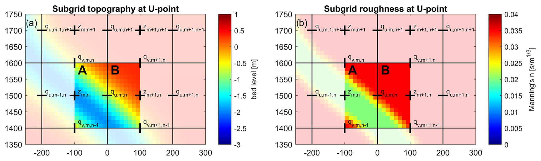
Figure 1 High-resolution values of elevation, z (a), and roughness, n (b), at a velocity point U, with a subgrid pixel resolution of $N=\mathrm{16}\times \mathrm{16}$ per computational cell. Colors for elevation and roughness indicate subgrid-scale values which are aggregated on the computational black grid cells. Water level points are indicated by +, while velocity points are marked with – and |.

For each velocity point (u here), we distinguish between two sides, A and B, of a computational cell (see Fig. 1). The minimum ($z_{\mathrm{b},\mathrm{A},\min }$ and $z_{\mathrm{b},\mathrm{B},\min }$) and maximum ($z_{\mathrm{b},\mathrm{A},\max }$ and $z_{\mathrm{b},\mathrm{B},\max }$) pixel elevations on both sides are determined. The combined minimum and maximum elevations, z_min and z_max, are defined as

$$\begin{array}{}\text{(14)}& {\displaystyle }{z}_{\min }=max\left(z_{\mathrm{b},\mathrm{A},\min },z_{\mathrm{b},\mathrm{B},\min }\right),\text{(15)}& {\displaystyle }{z}_{\max }=max\left(z_{\mathrm{b},\mathrm{A},\max },z_{\mathrm{b},\mathrm{B},\max }\right).\end{array}$$

Values of 〈H_u〉_G, n_u, and φ_u are now computed for both sides, A and B, and the total cell at discrete equidistant vertical levels, ranging between z_min and z_max:

$$\begin{array}{}\text{(16)}& {\mathit{\phi }}_{\mathrm{u},m}={\displaystyle \frac{\mathrm{1}}{N}}\sum _{k=\mathrm{1}}^{N}p\left(z_m-z_{b,k}\right),\end{array}$$

where $p(z_m--z_k)$ is 1 for z_m>z_k and 0 for z_m≤z_k:

$$\begin{array}{}\text{(17)}& {\displaystyle }\langle H_{\mathrm{u}}{\rangle }_{\mathrm{G},m}={\displaystyle \frac{\mathrm{1}}{N}}\sum _{k=\mathrm{1}}^N\left(z_m-z_{b,k},\mathrm{0}\right),\text{(18)}& {\displaystyle }{n}_{\mathrm{u},m}={\displaystyle \frac{\langle H_{\mathrm{u}}{\rangle }_{\mathrm{G},m}^{\mathrm{5}/\mathrm{3}}}{\frac{\mathrm{1}}{N}{\sum }_{k=\mathrm{1}}^N{\left(max\left(z_m-\left(z_{b,k},z_{\min }\right),\mathrm{0}\right)/n_k\right)}^{\mathrm{5}/\mathrm{3}}}}.\end{array}$$

If M is the number of vertical levels, the vertical distance between each level is defined as $\mathrm{\Delta }z=(z_{\max }-z_{\min })/(M-\mathrm{1})$, and the elevation of each discrete level is $z_m=z_{\min }+(m-\mathrm{1})\mathrm{\Delta }z$ (in which m goes from 1 to M). The number (M) of discrete vertical levels is defined by the user. We have found that around 20 levels are typically sufficient to accurately describe the subgrid quantities 〈H_u〉_G, n_u, and φ_u as a function of water levels between z_min and z_max, and this method is used throughout this paper. However, it is recommended to do a sensitivity analysis in order to find an optimal number of vertical levels. This can be done by running multiple simulations with an increasing number of levels. As the number of levels increases, the simulation results eventually converge. Ideally, the number of vertical levels should not significantly alter the simulation results and still result in an acceptable file size of the subgrid table file.

The subgrid tables and resulting flux (panel d) for the velocity point depicted in Fig. 1, using M=20, are illustrated in Fig. 2. Red markers highlight the values at the discrete vertical levels.

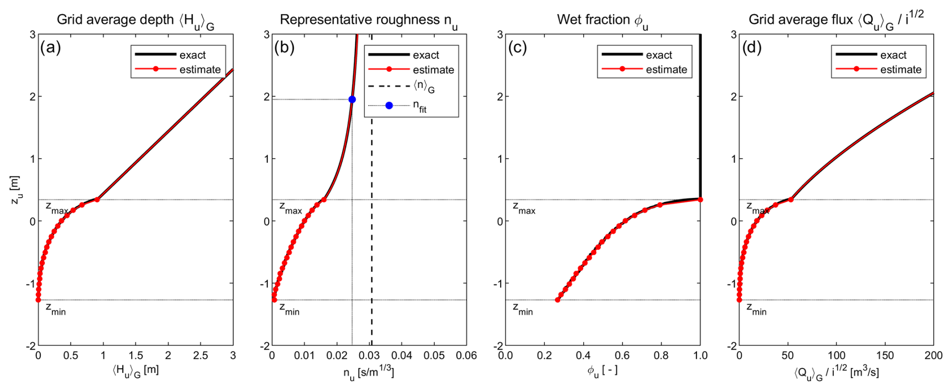
Figure 2 Computation of subgrid quantities 〈H_u〉_G (a), n_u (b) and φ_u (c) as a function of water level, z_u, with 20 discrete vertical levels (M=20). The resulting flux divided by the square root of the water slope, i, is shown in panel (d). The black line shows the exact solution obtained by solving Eqs. (5), (10), (11), and (17). The red line shows the estimate used in the SFINCS model, with (for z<=z_max) a linear interpolation of lookup table values and (for z>z_max) a linear increase for 〈H_u〉_G and fit for n_u.

Note that in Eq. (18), to determine the representative roughness, the maximum of the pixel elevation and z_min is used. This is done to ensure that when the water level, z_u, approaches z_min, i.e., when the highest of two adjacent grid cells becomes dry, n_u will become very large, thereby effectively blocking flow between sides A and B. No water is allowed to flow when z_u drops below z_min.

The determination of n_u for completely wet velocity points is more complicated due to its non-linear relationship with z_u at z_u>z_max (see Fig. 2b). It would be possible to store values of n_u at many levels above z_max in the subgrid tables, but that could result in file sizes that are too large and high memory use. To avoid this, SFINCS uses the following estimation for n_u instead:

$$\begin{array}{}\text{(19)}& n_{\mathrm{u}}=\langle n_{\mathrm{u}}{\rangle }_{\mathrm{G}}-{\displaystyle \frac{\langle n_{\mathrm{u}}{\rangle }_{\mathrm{G}}-n_{\mathrm{u},M}}{\mathit{\beta }\left(z_{\mathrm{u}}-z_{\max }\right)+\mathrm{1}}},\end{array}$$

where 〈n_u〉_G is the average Manning's n of all subgrid pixels and β is a fitting coefficient (with both of these parameters also stored in the subgrid tables). The fitting coefficient, β, is determined for each velocity point as

$$\begin{array}{}\text{(20)}& \mathit{\beta }={\displaystyle \frac{\frac{\langle n_{\mathrm{u}}{\rangle }_{\mathrm{G}}-n_{\mathrm{u},M}}{\langle n_{\mathrm{u}}{\rangle }_{\mathrm{G}}-n_{\mathrm{fit}}}-\mathrm{1}}{z_{\mathrm{fit}}-z_{\max }}}.\end{array}$$

Here we have defined the level z_fit at $z_{\max }+(z_{\max }-z_{\min })$. The value for n_fit at z_fit is determined in a manner similar to Eq. (18):

$$\begin{array}{}\text{(21)}& n_{\mathrm{fit}}={\displaystyle \frac{{\left(\langle H_{\mathrm{u}}{\rangle }_{\mathrm{G},M}+z_{\mathrm{fit}}-z_{\max }\right)}^{\mathrm{5}/\mathrm{3}}}{\frac{\mathrm{1}}{N}{\sum }_{k=\mathrm{1}}^N{\left(\frac{z_{\mathrm{fit}}-\left(z_{b,k},z_{\min }\right)}{n_k}\right)}^{\mathrm{5}/\mathrm{3}}}}.\end{array}$$

The estimated value for n_u above z_max using Eq. (19) is shown in Fig. 2b, with the blue marker indicating n_fit. In very deep water (z_u≫z_max), n_u approaches 〈n_u〉_G, whereas for z_u=z_max, n_u is equal to n_u,M.

The behavior of n_u in Fig. 2b can seem non-intuitive. Although the grid average water depth, 〈H_u〉_G, has a real physical meaning, the representative roughness, n_u, should not be interpreted as a physical quantity but rather as a quantity that is used to control the flux through a velocity point, given a certain grid average water depth 〈H_u〉_G and water slope i. It is a function of not only the physical subgrid roughness but also the subgrid water depth.

As mentioned previously, SFINCS uses grid average rather than wet average quantities. Theoretically, both options would yield identical results. The reason to choose a grid average approach is that the wet average depth and adjusted roughness can vary much more rapidly and irregularly with changing water levels than their grid average equivalents. As a result, many more vertical levels in the subgrid tables would be required to accurately describe wet average quantities as a function of z. This is illustrated by considering a velocity point with a subgrid topography cross section (Fig. 3a). The average water depth and adjusted roughness are derived as a function of water level, z (Fig. 3a and b, respectively).

At each time step the model computes the water level, z_u, at each velocity point using the maximum of the computed water levels in the two adjacent cells, i.e., $z_{\mathrm{u}}=\left(z_{sm,n},z_{sm+\mathrm{1},n}\right)$. This value is then used to query the lookup tables to find appropriate values of the quantities 〈H_u〉_G, n_u,m, and φ_u,m. For partially wet velocity points (z_min<z_u,m<z_max), a linear interpolation of the values in the tables is used. When the entire velocity point is wet (z_u≥z_max), the depth, 〈H_u〉_G, increases linearly with z_u:

$$\begin{array}{}\text{(22)}& \langle H_{\mathrm{u}}{\rangle }_{\mathrm{G}}=\langle H_{\mathrm{u}}{\rangle }_{\mathrm{G},M}+z_{\mathrm{u}}-z_{\max }.\end{array}$$

2.3 Subgrid corrections in the continuity equation

The subgrid continuity equation is written in terms of grid average fluxes as

$$\begin{array}{}\text{(23)}& \begin{array}{rl}{V}_{m,n}^{t+\mathrm{\Delta }t}& =V_{m,n}^{\mathrm{t}}+\mathrm{\Delta }t\left(\left(\langle q_{\mathrm{u}}{\rangle }_{\mathrm{G},m-\mathrm{1},n}^{\mathrm{t}}-\langle q_{\mathrm{u}}{\rangle }_{\mathrm{G},m,n}^{\mathrm{t}}\right)\mathrm{\Delta }y\right.\\ & \left.+\left(\langle q_{\mathrm{u}}{\rangle }_{\mathrm{G},m,n-\mathrm{1}}^{\mathrm{t}}-\langle q_{\mathrm{u}}{\rangle }_{\mathrm{G},m,n}^{\mathrm{t}}\right)\mathrm{\Delta }x+S_{m,n}\right).\end{array}\end{array}$$

Contrary to Eq. (2), Eq. (23) computes the wet volume at the next time step rather than the water level. The corresponding water level, z_s, is obtained from the continuity subgrid tables.

To generate the subgrid tables, first the minimum and maximum pixel elevations, z_min and z_max, and the wet volume, V_max (defined as the wet volume between z_min and z_max), are determined for each hydrodynamic grid cell (e.g., Fig. 3). The wet volume as a function of the local water level is then determined:

$$\begin{array}{}\text{(24)}& V\left(z\right)={\displaystyle \frac{\mathrm{\Delta }x\mathrm{\Delta }y}{N}}\sum _{k=\mathrm{1}}^N\left(z-z_k,\mathrm{0}\right),\end{array}$$

where N is the number of subgrid pixels in a grid cell. Finally, a number (M) of discrete equidistant volumes are defined, ranging between 0 and V_max, where each volume is $V_m=(m-\mathrm{1})V_{\max }/(M-\mathrm{1})$. By iterating over each discrete volume V_m, we can (using linear interpolation of Eq. 24) determine the corresponding water level z_s. An example is given in Fig. 3, which shows the volumes of the highlighted cell.

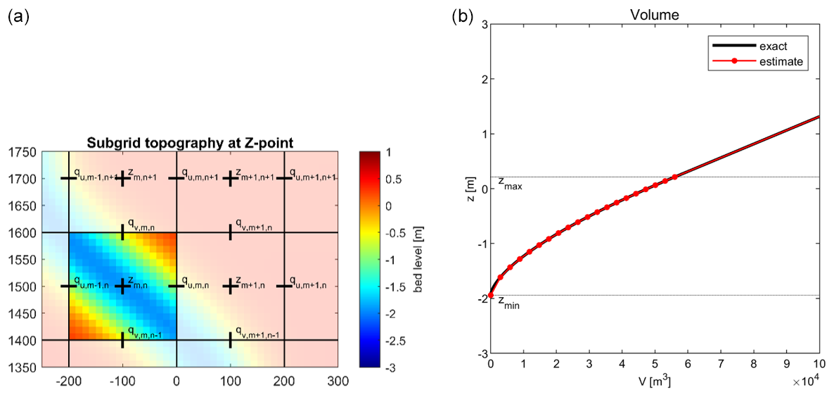
Figure 3 (a) Values on the subgrid-scale of elevation z at a water level point ($N=\mathrm{16}\times \mathrm{16}$). (b) Representation of water level, z_s, as a function of volume, V, with 20 discrete volumes (M=20). The black line shows the exact solution of Eq. (24). The red line shows the estimate of z_s used in the SFINCS model with, for z_s≤z_max, linear interpolation of lookup table values, and for z_s>z_max, a linear increase with V.

During a simulation, the model computes the volume V in each cell at each time step and queries the lookup tables to find the matching value for z_s. For partially wet cells (V<V_max), a linear interpolation of the values in the tables is used. When the entire cell is wet (V≥V_max), the water level z_s increases linearly with V and is computed as

$$\begin{array}{}\text{(25)}& z_s=z_{\max }+{\displaystyle \frac{V-V_{\max }}{\mathrm{\Delta }x\mathrm{\Delta }y}}.\end{array}$$

Note that for pre-processing purposes, it would have been more straightforward to describe the wet volume, V, at each equidistant vertical level z_m (similar to the approach for the momentum subgrid tables). However, during the simulation, the linear interpolation of subgrid data with equidistant volume levels is much more efficient.

The subgrid corrections in SFINCS are publicly available in the v2.1.1 Dollerup release (van Ormondt et al., 2024).

2.4 Pre- and post-processing

Pre-processing steps for SFINCS include creating a mask file describing (in)active cells, interpolating bathymetry and roughness values, and imposing boundary conditions. Tools to carry out these steps are available in both Delft Dashboard (van Ormondt et al., 2020) and HydroMT-SFINCS (Eilander et al., 2024, or https://deltares.github.io/hydromt_sfincs/latest/, last access: 1 April 2024), which both also have the capability to generate subgrid table files using high-resolution DEMs. In generating these subgrid tables, we largely follow common international standards such as NetCDF, ensuring compatibility and consistency with widely accepted practices in hydrodynamic modeling.

SFINCS stores the output of hydrodynamic quantities on the (coarse) computational grid. These results can be further downscaled to higher-resolution flood maps at the original DEM resolution (assuming again that the computed water level in a grid cell is representative of each subgrid pixel within that cell). Flood depths at the DEM scale are computed by subtracting the elevation of each DEM pixel from the water level in the cell. An example of the results is presented in Fig. 10.

3 Conceptual verification cases: straight and meandering channels

The first conceptual test involves a 5 km long straight channel of 100 m in width, with 1:5 side slopes (Fig. 4a and c) for which a synthetic bathymetry was created. The slope of the channel is 10⁻⁴ downhill in the y direction, and the floodplains on either side of the channel have an elevation of 0.3 m above the water level in the channel. Manning's n roughness is set to 0.02 s m${}^{-\mathrm{1}/\mathrm{3}}$. Water level boundary conditions at the upstream and downstream sides are set to +0.25 and −0.25 m, respectively, resulting in a 10⁻⁴ water level slope, equal to the channel slope. The analytical solution, using Manning's equation for open channel flow, yields a discharge of 360 m³ s⁻¹. The input files for the 5 m subgrid version of this model setup can be found in Appendix B1.

The second test is identical to the first, except that it has a meandering channel. The meandering channel has a sinuosity, Ω, i.e., the ratio between the length along the channel (6603 m) and its straight-line length (5000 m), of 1.32 (see, e.g., Lazarus and Constantine, 2013, for background information on river sinuosity). As the water levels upstream and downstream of the channel are kept the same, the water level slope in the meandering channel is smaller by a factor Ω, resulting in a (lower) analytical discharge of 313 m³ s⁻¹.

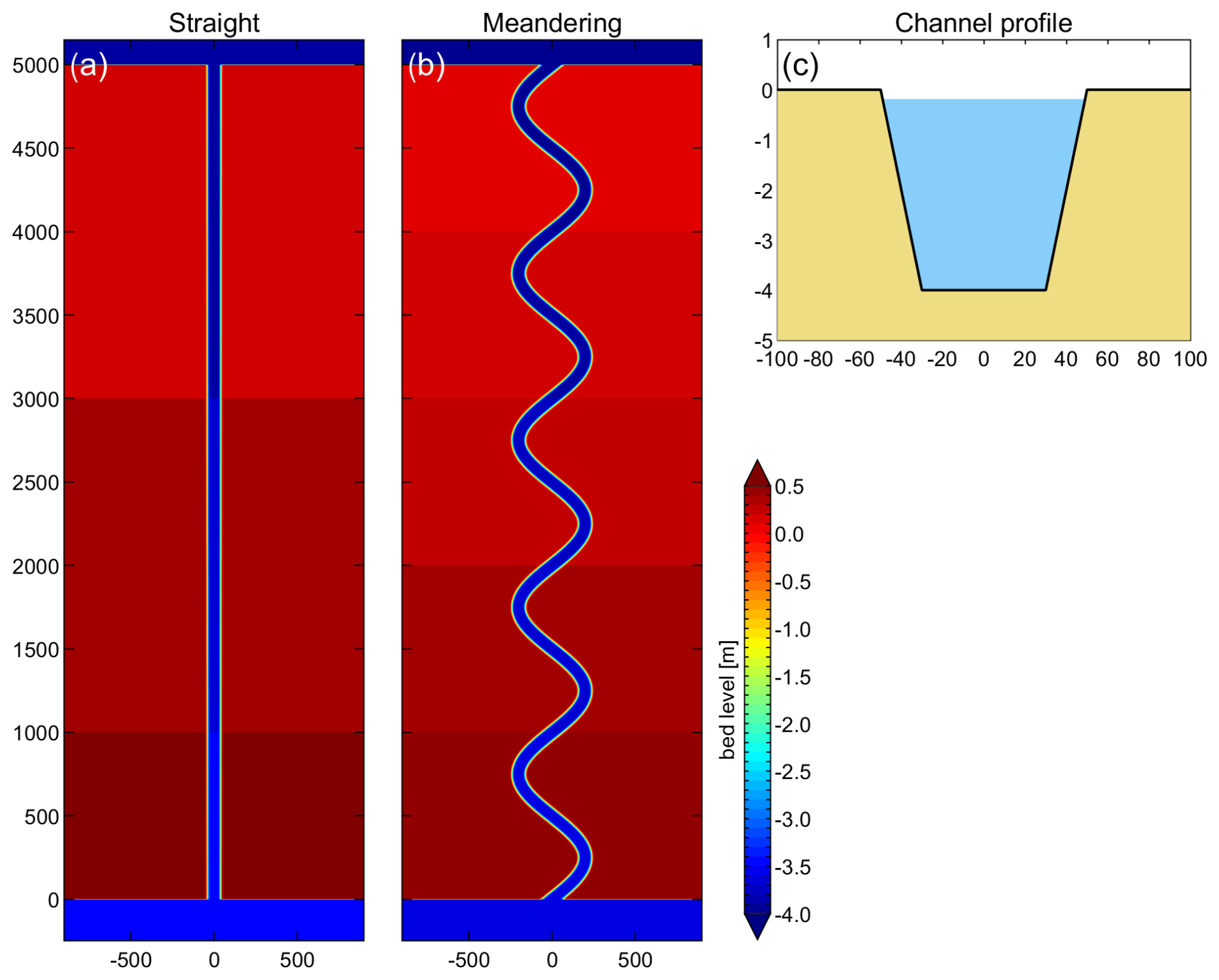
Figure 4 Schematized channel used in the conceptual verification cases, including a straight channel (top view, a), a meandering channel (top view, b), and a cross section (c).

Simulations are carried out at various grid resolutions (5, 10, 20, 50, 100, 200, and 500 m), with both subgrid and regular versions of SFINCS. The subgrid simulations use a 1 m resolution subgrid, onto which the DEM is bilinearly interpolated. For the regular topography simulations, grid cell averaging is used to schematize the model bathymetry in which the bed level of each cell is set equal to the mean of the DEM pixels within that cell. Figure 5 shows the regular model bathymetry at grid resolution, Δx, of 10, 50, and 200 m for the meandering channel. It is clear that although the first two capture the channel topography reasonably well, the channel depth in the 200 m model is strongly underestimated, and its width is proportionally overestimated.

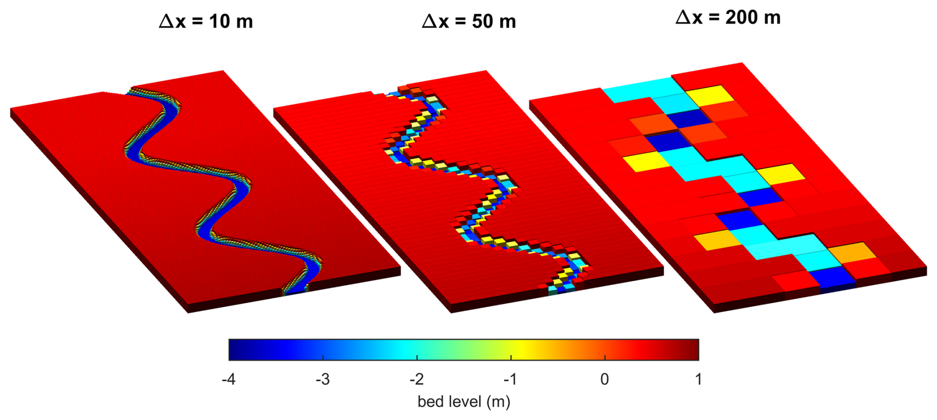
Figure 5 Schematized meandering channel bathymetry with regular topography for hydraulic grid resolutions of Δx=10 m, Δx=50 m, and Δx=200 m.

In the first test (straight channel), the regular bathymetry models stay reasonably close to the analytical solution up to resolutions of 50 m (blue bars in Fig. 6a). The accuracy of the coarser models, however, degrades significantly with a decreasing grid resolution, as is to be expected. The channel depth in the coarser models is increasingly underestimated, and even though its width is proportionately overestimated, the strongly non-linear relationship between water depth and discharge results in a decrease in the discharge with a decreasing grid resolution. In contrast, the discharge computed by the subgrid models is within 2 % of the analytical solution across all grid resolutions (red bars in Fig. 6a), proving that, at least for very simple conceptual cases, the subgrid corrections presented here are accurate.

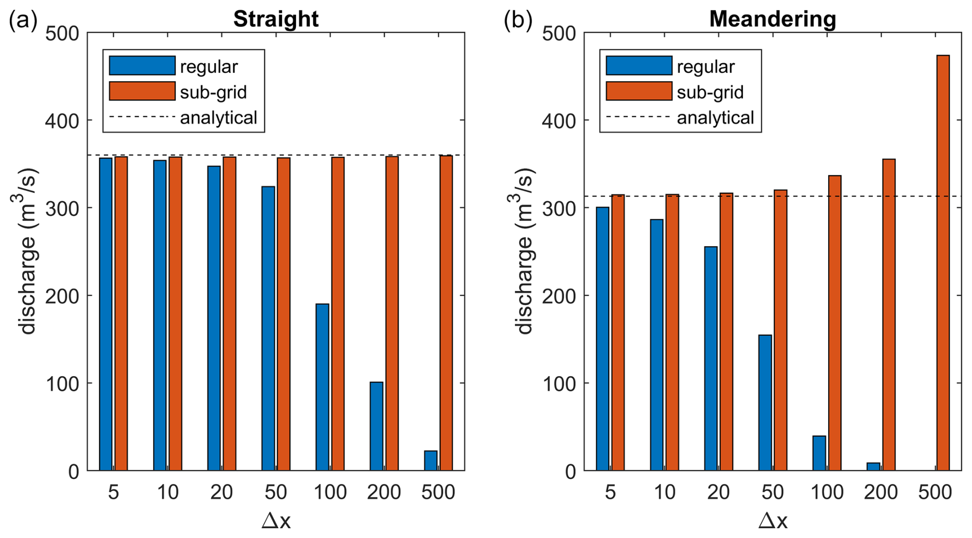
Figure 6 Effect of grid resolution, Δx, on computed discharges for regular and subgrid topography in a straight (a) and meandering (b) channel.

In the second test (meandering channel), the trend of the regular models is similar to those in the first test (blue bars in Fig. 6b), but the performance is lower than in the straight channel case, with the discharge for the two coarsest regular models going to zero. This is caused by the fact that the hydraulic connection between some channel cells is broken in the coarsest models (see also Fig. 5).

The subgrid models in the second test show a very good accuracy at resolutions up to 50 m. Coarser models start to overestimate the discharge. The 500 m model in particular computes a discharge of 473 m³ s⁻¹ (an overestimation of the analytical discharge by ∼ 51 %). There are two reasons for this: as the coarse mesh does not capture the scale of the meanders, the channel is effectively schematized as a straight channel with a length of 5000 m. This leads to an overestimation of the true water level slope and resulting wet average flux. Secondly, meanders inside a grid cell result in a larger wet fraction, which the model “interprets” as a wide channel, leading to a further overestimation.

For rivers with meanders that are not resolved by the model grid, we can approximate the discharge overestimation as a function of the channel sinuosity:

$$\begin{array}{}\text{(26)}& {\displaystyle \frac{Q_m}{Q_r}}={\mathrm{\Omega }}^{\mathrm{3}/\mathrm{2}},\end{array}$$

where Ω is the sinuosity, Q_r is the true discharge, and Q_m is the discharge computed with the subgrid corrections (see Appendix A for the derivation of Eq. 26). Equation (26) suggests that the discharge overestimation in the 500 m subgrid model (which does not resolve the meandering at all) is ∼ 52 % (${\mathrm{1.32}}^{\mathrm{3}/\mathrm{2}}$), which closely matches the computed overestimation of ∼ 51 % reported earlier.

4 Real-world application cases

4.1 Tidal propagation along St. Johns River

Leijnse et al. (2021) described SFINCS model results for Hurricane Irma (2017) along St. Johns River (Florida, USA). The length of the river is about 170 km from its mouth to Lake George upstream (Fig. 7a), where a small tidal signal still remains. Its width varies between 400 m and 5 km. Although the model showed good skill when compared to a full-physics Delft3D model, its 100 m grid resolution proved insufficient to adequately propagate the tide into the estuary.

In this test case, the St. Johns River SFINCS model from Leijnse et al. (2021) is adapted, and tidal propagation into the river is simulated at several horizontal resolutions (25, 50, 100, 200, and 500 m) using both the regular and the subgrid version of SFINCS. The topography and bathymetry data are improved using data obtained from the Continuously Updated Digital Elevation Model (CUDEM; CIRES, 2014). The Manning friction coefficient in the river is set to 0.02 s m${}^{-\mathrm{1}/\mathrm{3}}$. The offshore boundary water levels are derived from TPXO 8.0 tidal components (Egbert and Erofeeva, 2002). Computed water levels are validated against observed tidal components from 11 tide stations (retrieved through Delft Dashboard; van Ormondt et al., 2020) (Fig. 7a). The input files for the 25 m subgrid version of this model setup can be found in Appendix B2. In the subgrid version, we included a set of typical 20 discrete vertical levels to describe the subgrid quantities.

Simulations were carried out over a 1-month period to assess the model's capability to propagate the tide into the river. Analysis of the main tidal component M₂ across different model variations reveals considerable differences in the upstream propagation (Fig. 7b). The amplitude of M₂ is approximately 75 cm at the offshore boundary and sharply decreases near the city of Jacksonville, where the river narrows significantly (about 40 km upstream along the river). At a 100 m resolution, the SFINCS model with regular topography can reproduce the main trends but underestimates the tidal amplitudes relative to observations (Fig. 7b), as in Leijnse et al. (2021). At the coarser 500 m resolution, this underestimation of amplitude is significantly stronger, and the tide arrives too late (Fig. 7c). Tidal propagation only accurately matches the observations when utilizing a 25 m resolution with the regular topography.

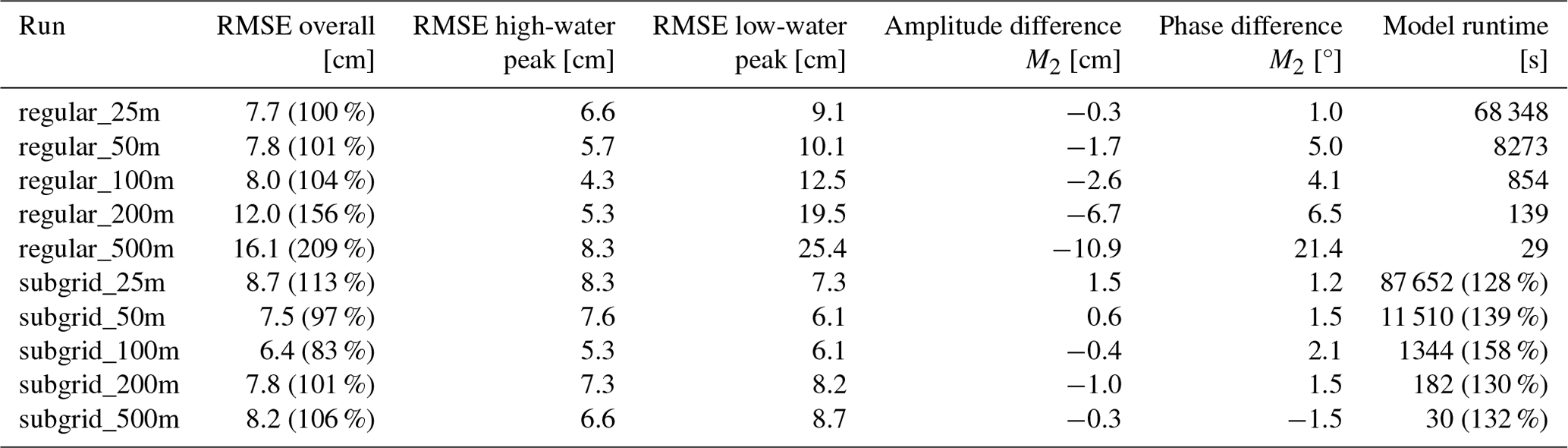
The subgrid version of SFINCS, on the same 100 m grid resolution, mitigates the underestimation of the regular (non-subgrid) version (Fig. 7b). The median error in M₂ amplitude prediction over the 11 observation stations decreases from 2.6 to 0.4 cm, the phase error from 4.1 to 2.1°, and the overall RMSE from 8.0 to 6.4 cm. Further analysis of different grid resolutions via the subgrid corrections illustrates that, even with coarser grid resolutions, the subgrid version of SFINCS propagates the tide inland properly even at very coarse resolutions of 500 m. Tidal phasing is also generally more accurately resolved with the subgrid versus regular SFINCS mode. Computing the RMSE over the whole month of tidal prediction shows that error increases from about 8 to about 20 cm for coarser grid resolutions in the regular SFINCS mode. However, when incorporating subgrid corrections, this remains stable around the value of 8 cm. While high-tide peak predictions remain robust for the subgrid SFINCS version at higher grid resolutions (Table 1), the performance decreases more significantly for low-water peaks, indicating that during these periods, the low-tide flushing of the river is still underestimated. Integrating the subgrid raises computational costs by around 28 %–58 % (37 % on average) as a result of the extra overhead involved in querying the subgrid tables. A comparison between the 25 m regular resolution and the 100 m subgrid resolution demonstrates similar skill but reveals a speedup of a factor 50, allowing the subgrid version to use coarser model resolutions with significantly lower computational costs without sacrificing precision.

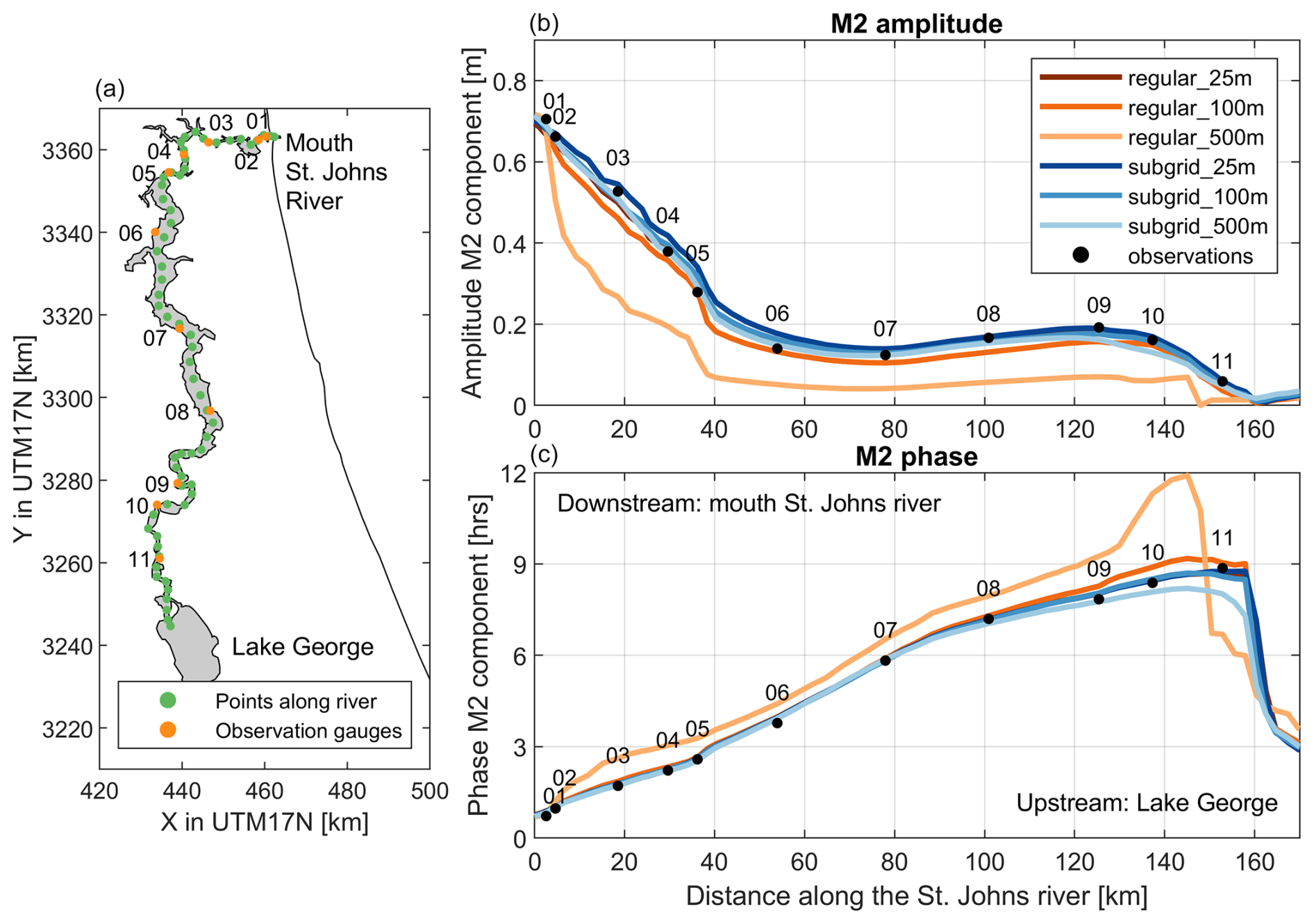
Figure 7 Overview of St. Johns River near Jacksonville, FL, USA (a), with analysis points (green dots) and tide gauges (yellow dots). (b) Observed (black dots) and modeled (colors) M₂ tidal amplitudes along the river from downstream to upstream. (c) Observed (black dots) and modeled (colors) M₂ tidal phases along the river. Different colors represent variations in the SFINCS model setup: red indicates the regular non-subgrid version, while blue denotes the subgrid version, with decreasing color intensity indicating a decrease in model resolution. The M₂ phase is converted from degrees to hours using the relation 1° $=\mathrm{12.42}h/\mathrm{360}$ (i.e., 0.0345 h per degree). The coordinate system is WGS 84/UTM 15N (EPSG 32615).

Table 1 Overview of model skill and computational expense for evaluated scenarios of inland tidal propagation at St. Johns River, FL. Metrics include RMSE of overall difference in time series compared to observations, RMSE of high-water peaks, RMSE of low-water peaks, difference in M₂ amplitude, and difference in the M₂ phase, all presented as medians over 11 observation stations. The last column shows the runtime in seconds, measured on an Intel Core i9-10980XE CPU. Each simulation was run three times, and the minimum runtime was recorded to eliminate potential contamination of timing. Additionally, the relative error in the regular 25 m configuration has been computed for the overall RMSE to provide further insight into the performance of the subgrid version of SFINCS compared to the baseline model. We also computed the percentage increase in computational costs for the subgrid version, which is reflected in the model runtime column to illustrate the additional computational expense. We also computed the percentage increase in computational costs for the subgrid version relative to the regular version, which is reflected in the model runtime column to illustrate the additional computational expense.

4.2 Pluvial flooding during Hurricane Harvey

Sebastian et al. (2021) used SFINCS to hindcast the flood extent and flood depth during Hurricane Harvey (2017) in Houston, TX. The model was validated against water level time series at 21 United States Geological Survey (USGS) observation points and 115 high-water mark (HWM) locations (Fig. 8). The original model was run with a regular 25 m resolution grid based on a high-resolution continuous topo-bathymetry across the area of interest. The model was compared to observed data across the study area, achieving an average error of 73 cm.

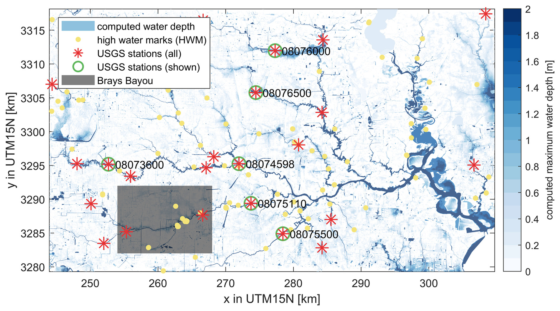
Figure 8 Modeled flood inundation in the urban areas of Houston, TX, simulated with SFINCS at a 25 m resolution with subgrid corrections. Water depths of less than 0.10 m are excluded for clarity. USGS stream gauges (red stars) and high-water marks (HWMs, yellow circles) used for model validation are shown as solid circles. Six USGS stations, presented as time series in Fig. 9, are marked with green circles, including their station numbers. A zoom-in of the midstream portion of Brays Bayou is shown in Fig. 10. The coordinate system is WGS 84/UTM 15N (EPSG 32615). © Microsoft.

In this field case, the model setup is adapted, and flooding across Houston is simulated at several horizontal resolutions. In particular, three variations for regular SFINCS (25, 50, and 100 m) and five variations in the subgrid (same resolutions as regular mode, including 200 and 500 m) were created. Model settings were based on the Sebastian et al. (2021) model except for the model resolution. Friction and infiltration capacity were cell-averaged from the original setup for the coarser model runs. The input files for the 25 m subgrid version of this model setup can be found in Appendix B3. In the subgrid version, we included higher-than-typical 100 discrete vertical levels to describe the subgrid quantities since during testing model skill improved when more vertical levels were included.

Almost all model versions reproduce the general shape of the observed hydrograph. However, the coarser regular version of SFINCS results in larger errors, mainly due to an overestimation of the water level (Fig. 9). The overestimation is driven by an incorrect representation of the bed level, which is averaged across larger areas and can therefore not depict the local bayous with coarser grid cells. SFINCS with the subgrid corrections improves the model skill (Table 2). For example, when comparing the 25 m regular version with the subgrid version of SFINCS on the same computational resolution, the Nash–Sutcliffe efficiency (NSE¹) increases from 0.35 to 0.58. NSE is a statistical metric used to evaluate the predictive accuracy of models by comparing observed and predicted values. NSE values range from 0 to 1, with values closer to 1 indicating a better-performing model. An NSE value of 0 means the model's predictions are as accurate as using the mean of the observed data as the predictor. Model skill increases because more topo-bathymetry information is considered per grid cell via the subgrid correction in the momentum and continuity equations (see Sect. 2.2 and 2.3). Despite the subgrid correction, model skill still decreases with a decreasing computational resolution. For example, a 500 m simulation with subgrid correction has an NSE of close to zero. Including the subgrid feature increases computational expense by 87 % to 175 % (average of 128 %) because of additional overhead in querying the subgrid tables. The highest model skill is obtained with the finest model resolution (25 m used here) including the subgrid. Selecting the model resolution is a balancing act between model skill and computational expense.

SFINCS can store the maximum computed water level across the computational domain, with the capability to downscale these data to higher-resolution flood maps as part of a post-processing step. In particular, to calculate flood depths at the DEM scale, the elevation of individual DEM pixels is subtracted from the corresponding cell's water level (see Sect. 2.4). For instance, the results demonstrate that the 25 m resolution outcomes and those downscaled to a 100 m subgrid are quite similar. This is illustrated in Fig. 10, which shows modeled flood inundation in the midstream portion of Brays Bayou using four different SFINCS model options. Panels a and c in Fig. 10 highlight the comparison: panel a presents the regular 25 m resolution, while panel c depicts the “subgrid 100m – downscaled” method, which applies a downscaling method to the DEM resolution as a post-processing step. However, the 100 m subgrid resolution runs 35 times faster than the 25 m regular SFINCS version while maintaining a similar level of accuracy (see Table 2), thus producing comparable extents of flooding. Nonetheless, it is important to note that the 100 m resolution results tend to provide a coarser visual representation of flood extents, often overestimating them (see panels b and d in Fig. A1) for both regular and subgrid versions of SFINCS.

Table 2 Overview of model skill and computational expense for evaluated scenarios of pluvial flooding during Harvey. Model skill metrics for time series, including NSE (Nash–Sutcliffe efficiency), MAE (mean absolute error), RMSE (root mean square error), and bias, as well as MAE for high-water marks (HWMs). The last column shows the runtime in seconds, measured on an Intel Core i9-10980XE CPU. Each simulation was run three times, and the minimum runtime was recorded to eliminate potential contamination of timing on Windows. Additionally, the relative MAE to the regular model configuration has been computed to provide further insight into the performance improvements with the subgrid corrections. We also computed the percentage increase in computational costs for the subgrid version, which is reflected in the model runtime column to illustrate the additional computational expense.

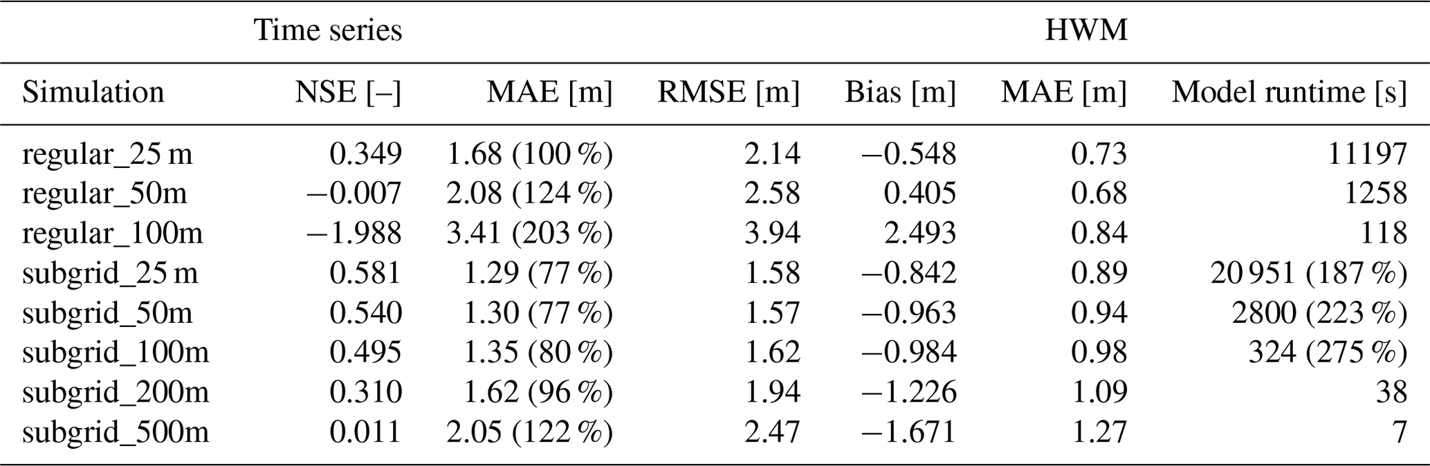
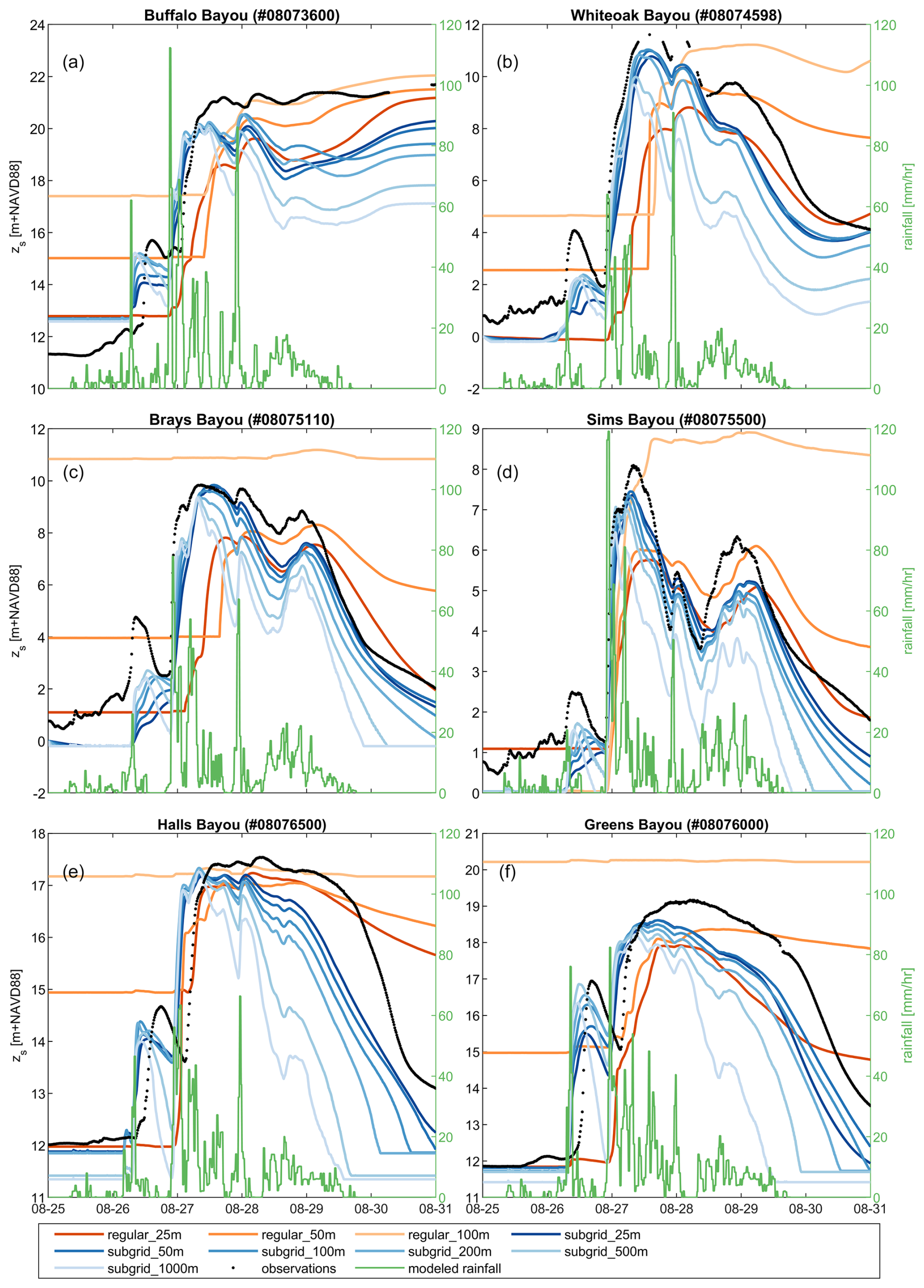
Figure 9 Overview of (computed) water levels during Hurricane Harvey. Comparison between modeled (colored lines) and observed (black lines) hydrographs at six USGS gauge locations (labeled in Fig. 8): (a) Buffalo Bayou (USGS 08073600); (b) White Oak Bayou at Main Street (USGS 08074598); (c) Brays Bayou at MLK Jr. Blvd (USGS 08075110); (d) Sims Bayou at Houston, TX (USGS 08075500); (e) Vince Bayou at Houston, TX (USGS 08075730); and (f) Greens Bayou nr Houston, TX (USGS 08076000). Different colors represent variations in the SFINCS model setup. Red is used for the regular version of SFINCS (non-subgrid). Blue is used for the subgrid version of SFINCS. Decreasing color intensity depicts a decrease in model resolution. Rainfall intensity is included as the green line and uses the right y axis.

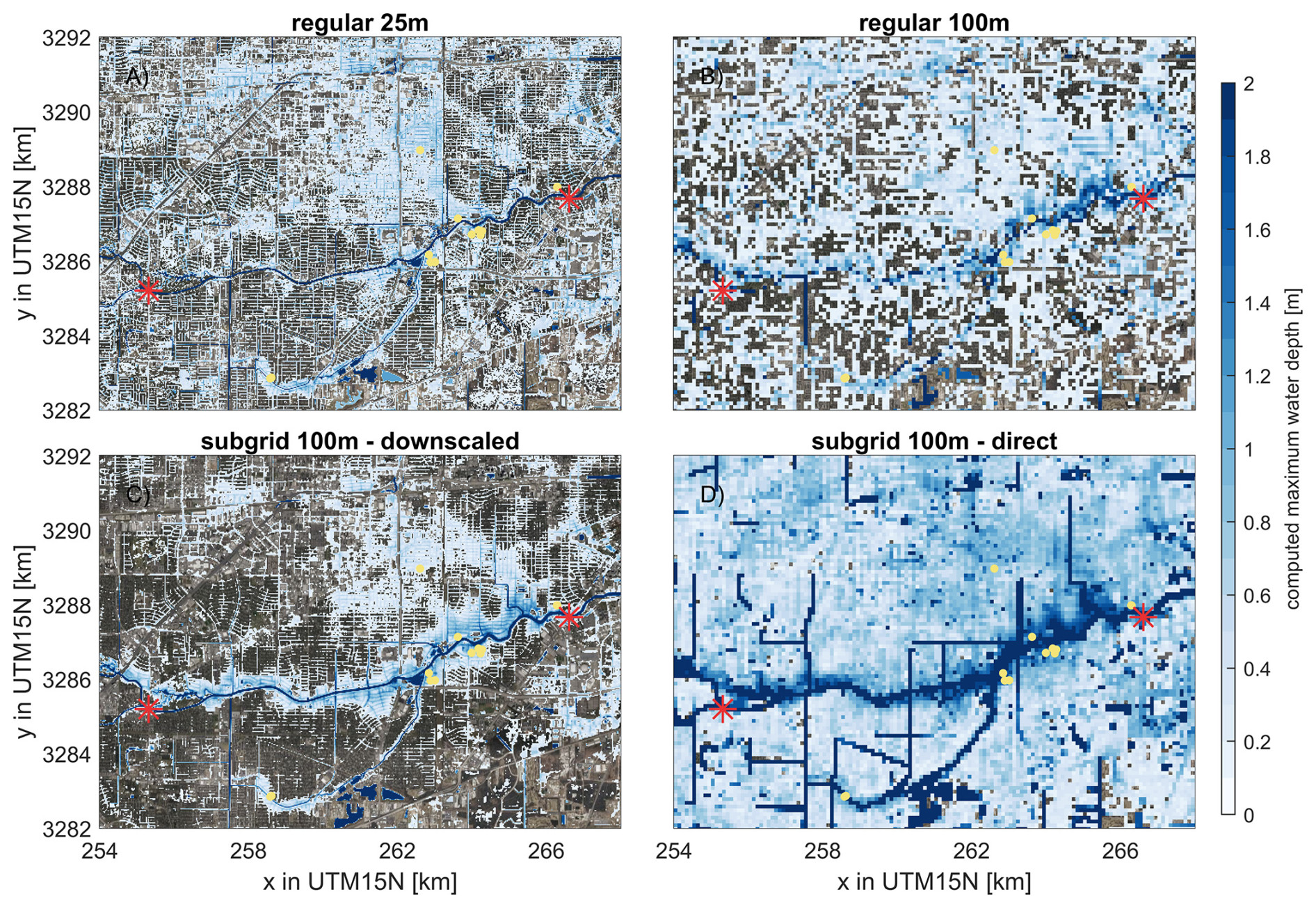
Figure 10 Modeled flood inundation in the midstream portion of Brays Bayou for four different SFINCS model options: (a) regular 25 m; (b) regular 100 m; and (c) “subgrid 100m – downscaled”, using the same model simulation as “subgrid 100m – direct” (d) but then applying a downscaling method to the DEM resolution as a post-processing step. Water depths lower than 0.10 m have been excluded for visual purposes. The locations of USGS stream gauges (red stars) and HWMs (yellow circles) used for the model validation are shown. The coordinate system of this figure is WGS 84/UTM 15N (EPSG 32615). © Microsoft.

5 Discussion

The integration of subgrid corrections into SFINCS has led to significant enhancements in accuracy, as evidenced in both conceptual verification cases (Sect. 3) and real-world scenarios, including tidal propagation (Sect. 4.1) and pluvial flooding (Sect. 4.2). This section delves into the impact of these accuracy enhancements and outlines the remaining challenges and areas for future research, particularly concerning flow-blocking features and the overestimation of fluxes in meandering systems.

The ability to achieve improved accuracy with the same grid resolution signifies progress. However, in practical terms, a more accurate simulation also allows for the use of coarser model resolutions. This is particularly advantageous given SFINCS's explicit numerical scheme, enabling faster and thus more efficient compound flood modeling. For example, in the real-world application cases of tidal propagation (Sect. 4.1) and pluvial flooding (Sect. 4.2), a subgrid model at a 100 m resolution demonstrates comparable, if not higher, performance to the regular 25 m resolution SFINCS model. However, the computational cost is significantly lower, with a speedup of a factor of 35–50. The introduction of subgrid corrections does introduce additional computational expenses versus regular SFINCS for the same grid spacing. In the St. Johns River case (Sect. 4.1), where we used 20 discrete bins to describe the subgrid quantities, the increase in computational costs was relatively low, with an average increase of 37 % when comparing the same grid spacing. In contrast, higher costs were observed in the Hurricane Harvey case (Sect. 4.2), where model performance improved when 100 discrete bins were used instead of the more typical 20 bins, leading to an average computational cost increase of 128 %. Therefore, the increase in computational costs is dependent on the number of bins used to describe the subgrid quantities, with finer binning sometimes providing better accuracy at the cost of increased computational demands. Additionally, using more bins also results in larger NetCDF subgrid files. For example, in the 200 m Harvey case, the subgrid file size was 343 MB, compared to 65 MB for the 200 m Jacksonville case, a nearly 6-fold increase. Notably, the number of active cells was twice as large for the Jacksonville case, which demonstrates that subgrid file sizes scale linearly as a function of the number of both active cells and discrete bins.

The downscaling routines implemented also allowed for the use of the high-resolution data in the post-processing step. However, the simple subtraction of the computed water level and high-resolution topography (introduced in Sect. 2.4 and applied in Sect. 4.2) might result in water in an area that would not be flooded using high-resolution models. While this might not affect the accuracy compared to water level stations, it does influence results and flood extents. In particular, disconnected grid cells might pop up behind levees and other flow-breaking features which form a challenge when communicating the results to stakeholders. Moreover, the presented downscaling routine has limited use for areas with steep gradients where the assumption of a constant water level per computational cell is invalid. Therefore, exploring more sophisticated hybrid surrogate models might improve the dynamic evolution of the flood extent (Fraehr et al., 2022). Furthermore, in the subgrid SFINCS model, we estimate infiltration rates on the computational grid. This approach does not account for higher-resolution information in the estimation of infiltration rates, which may lead to less accurate representations of infiltration in areas where high-resolution variability is significant. Future work could explore integrating finer-scale soil and topographic data into the infiltration estimation process to further enhance the model's performance, particularly in regions with partial wet cells and heterogeneous soil properties.

It is important to note that the real-world cases evaluated here are not without limitations. One ongoing challenge for the modeling community is the insufficient representation of river bathymetry in combined topo-bathymetry datasets. In many cases, river bathymetry is not well captured, which can affect the accuracy of hydrodynamic models, particularly for riverine flooding. Furthermore, land cover maps used to estimate bed friction can introduce contamination, affecting model accuracy. No specific adjustments were made to the real-world cases presented in this paper, and the published models were simply adjusted to be run at several resolutions with and without subgrid corrections.

Addressing subgrid connectivity poses a significant challenge for the implementation described in this paper and the broader modeling community. In contrast to approaches that relied on cell and edge clones (Casulli, 2009b; Begmohammadi et al., 2021) or artificial diffusion (Rong et al., 2023), SFINCS employs a subgrid weir formulation. This formulation, which is aligned with (or snapped to) the grid, controls the flow between two cells but requires the creation of subgrid features during a pre-processing phase. To date, these features have been manually identified. However, there is ongoing research into algorithms capable of detecting flow-blocking features as well as the integration of methods from existing literature or direct modifications to the subgrid lookup tables to account for this. In scenarios where flow-blocking features (such as levees or urban structures) are not adequately captured, the model may underestimate the extent of localized flooding.

Similarly, the overestimation of fluxes in situations with unresolved meanders continues to be a challenge. This issue is not exclusive to SFINCS's implementation of subgrid corrections but is a common challenge across subgrid modeling. Various estimates for the sinuosity, Ω, have been reported in scientific literature. Lazarus and Constantine (2013) suggest that the typical range for Ω lies between 1 and 3, where 1 corresponds to a straight channel and 3 represents the upper limit for natural, freely migrating meandering rivers. Hence, when using a computational grid that does not resolve the river meanders, the presented subgrid corrections may overestimate discharges by more than a factor of 5 (or 3${}^{\mathrm{3}/\mathrm{2}}$). This is especially important in real-world scenarios involving highly sinuous river systems, where discharge inaccuracies can significantly affect flood predictions. To mitigate this, it is recommended that the grid spacing of the computational grid does not exceed the width of the river channel.

6 Conclusions

Large-scale flood models require high accuracy at acceptable computational times. One strategy to achieve this is to use information available at a resolution higher than the hydrodynamic grid resolution in models through subgrid corrections. This paper describes a set of subgrid corrections to the linear inertial equations (LIEs) using grid average quantities (depth, representative roughness, wet fraction, and flux to the momentum equations and for the wet volume in the continuity equation) which were implemented in SFINCS. The model uses pre-processed subgrid tables that correlate water levels with hydrodynamic quantities by assuming constant water levels for all subgrid pixels.

The conceptual case of a straight channel showed good skill in terms of discharge fluxes with the subgrid model regardless of the model resolution, while the accuracy of the regular models without subgrid correction decreased significantly with decreasing resolution. For the meandering channel, differences start to emerge for coarser model resolutions with and without subgrid corrections. In particular, the difference in discharge estimation was overestimated by 50 % for the coarsest subgrid model used. The ratio between the length along the channel and its straight-line length (also known as sinuosity or Ω) served as a valuable metric for quantifying flux overestimations. The conceptual cases gave confidence that the corrections were correctly implemented while also highlighting their limitations in grids that do not adequately resolve river meanders. In particular, we introduced an equation that allows for the approximation of discharge overestimation as a function of the channel sinuosity.

Real-world application cases further validated the benefits of subgrid corrections. For tidal propagation in St. Johns River, the subgrid model with a 500 m resolution matched the accuracy of the 25 m standard SFINCS model. Similarly, in modeling pluvial flooding during Hurricane Harvey, a 25 m resolution SFINCS model was necessary to achieve a Nash–Sutcliffe efficiency (NSE) of 0.35, while the subgrid variant at the same resolution outperformed this with an NSE of 0.58 (where a score of 1 would be perfect) and maintained comparable accuracy even at a coarser 100 m resolution. Although subgrid corrections introduce additional computational costs – ranging from 37 % to 128 % depending on binning density – they provide significant benefits in performance and accuracy, achieving a speedup of a factor of 35–50 by enabling the use of coarser resolutions and thus improving efficiency in real-world flood modeling applications.

Building on these findings, the implementation of subgrid corrections for LIEs within SFINCS demonstrates significant potential for improving accuracy and reducing computational demands in compound flooding simulations. However, the broader relevance of subgrid corrections should not be limited to LIEs or SFINCS alone. Subgrid corrections could benefit a wide range of hydrodynamic models, such as full-physics or reduced-complexity models alike, Furthermore, these corrections could be applied across diverse environmental conditions, including urban pluvial flooding, coastal storm surge, and riverine flooding, thereby enhancing the generalizability and utility of hydrodynamic modeling across various domains. Overall, the results from both conceptual and real-world cases show that subgrid corrections are a valuable addition to hydrodynamic modeling, particularly when balancing the need for accuracy with computational efficiency.

Appendix A: Derivation of discharge overestimation due to unresolved meandering

The subgrid corrections presented in this paper may result in an overestimation of fluxes between grid cells in places where river meanders are not sufficiently resolved by the computational grid. The overestimation may be expressed as the ratio between the computed and theoretical fluxes. In this appendix, we describe a simple relation between this ratio and the river sinuosity in cases where the model grid does not resolve the meanders at all. The sinuosity is defined as the ratio between the length along the channel and its straight-line length (e.g., Lazarus and Constantine, 2013).

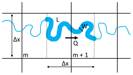
Figure A1 Conceptual figure of the sinuosity, which is a defined as the ratio between the length along the channel and its straight-line length.

Using Manning's formula, the theoretical discharge can be described by

$$\begin{array}{}\text{(A1)}& Q_r={\displaystyle \frac{W\sqrt{\frac{\mathrm{\Delta }z}{L}}{H}^{\mathrm{53}}}{n}},\end{array}$$

where W is the river width, L is the length of the center line of the river stretch, Δz is the water level difference over the river stretch, H is the channel depth (assumed uniform), and n is Manning's roughness coefficient.

Inside a model using the subgrid corrections, the discharge computed at the cell interface is

$$\begin{array}{}\text{(A2)}& Q_m=\mathrm{\Delta }x{\displaystyle \frac{\mathit{\phi }\sqrt{\frac{\mathrm{\Delta }z}{\mathrm{\Delta }x}}{H}^{\mathrm{53}}}{n}},\end{array}$$

where Δx is the grid size, φ is the wet fraction of the velocity point, and H is the wet average depth.

We assume here that the sinuosity is

$$\begin{array}{}\text{(A3)}& \mathrm{\Omega }={\displaystyle \frac{L}{\mathrm{\Delta }x}}\end{array}$$

Furthermore, the wet fraction, φ, in Eq. (A2) can be defined as the river area, W×L, divided by the cell area:

$$\begin{array}{}\text{(A4)}& \mathit{\phi }={\displaystyle \frac{WL}{\mathrm{\Delta }{x}^{\mathrm{2}}}}={\displaystyle \frac{W}{\mathrm{\Delta }x}}\mathrm{\Omega }.\end{array}$$

After substituting φ in Eq. (A2) with Eq. (A4), we can write the overestimation (i.e., the ratio of the computed and theoretical discharge, Q_m / Q_r), as

$$\begin{array}{}\text{(A5)}& {\displaystyle \frac{Q_m}{Q_r}}={\displaystyle \frac{\mathrm{\Delta }x\frac{\frac{W}{\mathrm{\Delta }x}\mathrm{\Omega }\sqrt{\frac{\mathrm{\Delta }z}{\mathrm{\Delta }x}}{H}^{\mathrm{5}/\mathrm{3}}}{n}}{\frac{W\sqrt{\frac{\mathrm{\Delta }z}{L}}{H}^{\mathrm{53}}}{n}}}=\mathrm{\Omega }\sqrt{{\displaystyle \frac{L}{\mathrm{\Delta }x}}}=\mathrm{\Omega }\sqrt{\mathrm{\Omega }}={\mathrm{\Omega }}^{\mathrm{3}/\mathrm{2}}.\end{array}$$

Appendix B: Input files for cases considered in this paper

B1 Conceptual verification cases: straight and meandering channels

mmax	11
nmax	26
dx	200
dy	200
x0	−1000
y0	0
rotation	0
tref	20190101 000000
tstart	20190101 000000
tstop	20190103 000000
tspinup	60
dtout	3600
dthisout	600
dtmaxout	3600
alpha	0.5
theta	0.95
huthresh	0.005
zsini	1
qinf	0
rhoa	1.25
rhow	1024
advection	1
depfile	sfincs.dep
mskfile	sfincs.msk
indexfile	sfincs.ind
bndfile	sfincs.bnd
bzsfile	sfincs.bzs
srcfile	sfincs.src
disfile	sfincs.dis
sbgfile	sfincs_subgrid.nc
obsfile	sfincs.obs
crsfile	sfincs.crs
manningfile	sfincs.manning
inputformat	bin
outputformat	net
storevelocity	1
storevel	1

B2 Tidal propagation along St. Johns River

mmax	2720
nmax	5520
dx	25
dy	25
x0	459437
y0	3375791
rotation	−164
epsg	32617
latitude	0
tref	20180901 000000
tstart	20180901 000000
tstop	20180931 000000
tspinup	60
dtout	86400
dthisout	600
dtmaxout	99999999999
trstout	-999
alpha	0.5
theta	1
huthresh	0.01
manning_land	0.04
manning_sea	0.02
rgh_lev_land	0
zsini	0
qinf	0
rhoa	1.25
rhow	1024
advection	1
btfilter	60
viscosity	1
depfile	sfincs.dep
mskfile	sfincs.msk
indexfile	sfincs.ind
bndfile	.sfincs.bnd
bzsfile	sfincs.bzs
sbgfile	sfincs_subgrid.nc
obsfile	noaa_xtide_v4_added_debug_points.obs
inputformat	bin
outputformat	net

B3 Pluvial flooding during Hurricane Harvey

mmax	2632
nmax	1555
dx	25
dy	25
x0	243943.5
y0	3279280
rotation	0
epsg	32615
tref	20170825 000000
tstart	20170825 000000
tstop	20170831 000000
dtout	86400
dthisout	600
dtmaxout	518400
dtwnd	600
alpha	0.5
theta	1
huthresh	0.05
rgh_lev_land	0
zsini	0
qinf	0
rhoa	1.25
rhow	1000
advection	1
depfile	sfincs.dep
mskfile	sfincs.msk
indexfile	sfincs.ind
bndfile	sfincs.bnd
bzsfile	sfincs.bzs
srcfile	sfincs.src
disfile	sfincs.dis
sbgfile	sfincs_subgrid.nc
amprfile	Observations_Interpolate_600x600_halfhour_test.ampr
obsfile	sfincs.obs
inputformat	bin
outputformat	net
qinffile	qinf_constanttime_spatialvary
storevel	1