age_flow_line-1.0: a fast and accurate numerical age model for a pseudo-steady flow tube of an ice sheet

Numerical age models are useful tools for investigating the age of the ice in an ice sheet. They can be used to date ice cores or to interpret isochronal horizons which are observed by radar instruments. Here, we present a new numerical age model for a flow line of an ice sheet. The assumption here is that the geometry of the flow line and the velocity shape functions are steady (i.e. constant in time). A time-varying factor can only be applied to the surface accumulation rates and basal melting rates. Our model uses an innovative logarithmic flux coordinate system (π, θ), previously published, which is suitable for solving transport equations because it tracks ice trajectories. Using this coordinate system, solving the age equation is simple, fast and accurate, because the trajectories of ice particles pass exactly through the nodes of the grid. Our numerical scheme, called Eulerian-Lagrangian, therefore combines the advantages of Eulerian and Lagrangian schemes. We present an application of this model to the flow line going from Dome C to the Beyond EPICA Little Dome C drill site and show that horizontal flow is a non-negligible factor which should be considered when modelling the age-depth relationship of the Beyond EPICA ice core. The code we developed for age modelling along a flow tube is named age_flow_line-1.0 and is freely available under an open-source license.

1 Introduction

Ice sheets, such as the current Greenland or Antarctic ice sheets, or the past Fennoscandian or Laurentide ice sheets, are a fundamental component of the global climate system (Oerlemans and Van Der Veen, 1984). They are the largest reservoir of fresh water on Earth (Vaughan et al., 2013; IPCC, 2019); their existence causes global sea level to be lower than it would otherwise be (Fyke et al., 2018); their white surfaces lead to a strong albedo which cools the regional and even global climates (Fyke et al., 2018); their high elevation modifies the atmospheric circulation (Fyke et al., 2018); and the fresh water and icebergs they release into the oceans can perturb the deep ocean circulation (Fyke et al., 2018). Therefore, it is essential to understand the processes and the boundary conditions which govern the evolution of ice sheets.

Current ice sheets are also an extraordinary archive of past climates. They can record local temperature variations when the snow fell (Jouzel et al., 2007; NorthGRIP project members, 2004), the past atmospheric composition (Loulergue et al., 2008; Lüthi et al., 2008) and atmospheric impurities (Lambert et al., 2012). For the interpretation of the ice core records, it is essential to date the ice and reconstruct the trajectories and mechanical histories of ice particles within the ice sheets.

Modelling the age and trajectories of the ice in ice sheets is important for several reasons. This includes dating existing ice cores and correcting from upstream effects (Buchardt, 2009; Huybrechts et al., 2007; Johnsen and Dansgaard, 1992; Parrenin et al., 2007). Ice cores can also be dated by counting annual layers where these layers are thick enough (Svensson et al., 2008) or by identifying dated horizons (Bouchet et al., 2023). But modelling also provides an estimate of the thinning and horizontal displacement of ice layers. For example, moving down in the EDML ice core, there is a decreasing trend in the ice isotopic record that corresponds to a decrease in atmospheric temperature during snow deposition. This decrease is not due to temporal climatic variations, but simply to the fact that deeper down, the ice originates from further upstream, from a higher elevation and therefore colder site (Huybrechts et al., 2007). Moreover, investigating new potential ice core drill sites (Chung et al., 2023; Obase et al., 2023; Parrenin et al., 2017; Van Liefferinge and Pattyn, 2013) usually requires some modelling since radar-observed isochrones generally do not cover the whole ice column. Age observations from ice cores (Bouchet et al., 2023; Oyabu et al., 2022) or from radio echo sounding (Cavitte et al., 2016; MacGregor et al., 2015) can also help constrain the boundary conditions of ice sheet models or understand the internal processes of ice sheets using inverse methods. For example, dated isochrones can help deduce the surface accumulation rate, the basal melting rate or the horizontal and vertical velocity profiles (Buchardt and Dahl-Jensen, 2007; Parrenin et al., 2017; Chung et al., 2023). Finally, modelling is necessary to estimate the age distribution across an ice sheet, since it is usually not covered entirely by observations. Key challenges in age modelling include numerical accuracy and efficiency, the match to observations and accounting for boundary conditions.

Various types of numerical models with a transport scheme to compute the age within the ice sheets have been developed. For example, large scale transient models have been used (Lhomme et al., 2005a; Sutter et al., 2019; Born and Robinson, 2021) to estimate the stratigraphy of the Greenland and Antarctic ice sheets. The advantages of these models are that they are fully transient and consider many of the different physical processes involved in ice sheet evolution. However, boundary conditions such as the geothermal flux, the basal drag or the surface accumulation rates for these models are poorly known. Due to their large computation time, the evolution equations are often simplified and their resolution is multi-kilometric, meaning that detailed bedrock relief is not/cannot be taken into account. Moreover, these models might simulate a present-day surface topography which is different from the observed surface topography, making it challenging to compare the model with existing ice core or radar observations. To improve the resolution or the representation of physical processes in these models, it is possible to embed a local high resolution and high order model within a simplified continental ice sheet model (Huybrechts et al., 2007).

Another approach is to use local 1D (purely vertical) or 2.5D (flow tube) models with a prescribed geometry. These models can be either transient (Koutnik et al., 2016; Obase et al., 2023), steady-state (Waddington et al., 2007) or pseudo-steady (Chung et al., 2023; Parrenin et al., 2017) which is a steady-state model but with a scaling of the age to account for the temporal change of surface accumulation rate.

There exist several numerical schemes for solving the transport equations, a class to which the age equation belongs (Rybak and Huybrechts, 2003). The Lagrangian scheme follows ice particles within their journey and is generally stable. However, the tracers are dispersed and it is not possible to know a priori where these tracers will end up at the end of the simulation. The Eulerian scheme solves the age equation on a grid and does not have the problem of tracer dispersion but can be numerically unstable, especially in 3D (Hindmarsh et al., 2009). The third numerical scheme is the semi-Lagrangian scheme, which, as with the Eulerian scheme, solves the age equation on a grid. It is more stable than the Eulerian scheme but suffers from numerical diffusion (Lhomme et al., 2005b; Sutter et al., 2021).

Here we present a new 2.5D (flow tube) pseudo-steady numerical age model, named age_flow_line-1.0. This numerical age model uses an innovative coordinate system (π, θ) previously published (Parrenin et al., 2006; Parrenin and Hindmarsh, 2007) and which is suitable for solving transport equations. We solve the age and spatial origin equations using a Eulerian-Lagrangian scheme that uses an analytical derivation of trajectories and a grid which tracks these trajectories. This model offers improved numerical accuracy and efficiency over existing models and is therefore appropriate for inverse methods where many forward simulations are necessary. In Sect. 2, we first present the analytical and numerical foundations of the model and its implementation. In Sect. 3, we show an application of the model to the flow line between Dome C (DC) and the Beyond EPICA Little Dome C (BELDC) ice coring site in Antarctica. In Sect. 4, we discuss the advantages and limitations of the model.

2 Description of the model

2.1 Notations and analytical aspects

We first consider a steady-state flow tube of an ice sheet, which starts at a dome and ends at the ice sheet margin (Fig. 1). This means that we assume that factors such as the geometry of the flow tube (e.g. ice thickness) and the vertical shape function do not change in time. In this model, we consider non-steady accumulation rate and melting rate, but this will be discussed later. The notation and equations follow that of Parrenin and Hindmarsh (2007) but the assumptions are slightly relaxed since we allow the flow tube width and relative density to vary vertically. We write the equations in the (x, z) coordinates where x, the horizontal coordinate along the direction of ice flow, is the distance from the dome and z is the vertical coordinate pointing upward. We suppose that the horizontal direction of the flow does not depend on the vertical position and is time-independent, and we represent the lateral flow divergence by the varying flow tube width Y(x,z). In practice, for grounded ice and under the shallow ice approximation, the direction of the flow can be determined from the surface elevation gradient. In this case, the steady-state assumption for the flow tube means that the shape of surface elevation contours does not change with time. The direction of the flow can also be determined by surface velocity measurements, as is done for the modelling of the flow line from DC to BELDC (Chung et al., 2025). Using surface velocity measurements is more appropriate where the surface is flat because in this case, the flow might not follow the direction of the greatest local slope.

The ice-sheet geometry is given by the bedrock elevation B(x), the surface elevation S(x) and the total ice thickness $H\left(x\right)=S\left(x\right)-B\left(x\right).$ We let snow/ice relative density (expressed in % of volume) be D(x,z) and the surface accumulation of ice and basal melting rate at the ice–bedrock interface be a(x) and m(x), respectively. We let u_x(x,z) denote the horizontal velocity and u_z(x,z) the vertical velocity of the ice particles. We also let χ(x,z) represent the age of the ice particle.

We now define fluxes used to derive the stream function. The partial horizontal flux q_H(x,z) is defined as the horizontal flux passing below elevation z:

$$\begin{array}{}\text{(1)}& q_{\mathrm{H}}(x,z)=\underset{B}{\overset{z}{\int }}Y(x,z^{\prime })D(x,z^{\prime })u_x(x,z^{\prime })\mathrm{d}{z}^{\prime }\end{array}$$

with $Q_{\mathrm{H}}\left(x\right)=q_{\mathrm{H}}(x,S)$ being the total horizontal flux at position x. We further define the basal melting flux as:

$$\begin{array}{}\text{(2)}& Q_{\mathrm{m}}\left(x\right)=\underset{\mathrm{0}}{\overset{x}{\int }}{Y}^{\mathrm{B}}\left(x^{\prime }\right)m\left(x^{\prime }\right)\mathrm{d}{x}^{\prime }\end{array}$$

where $Y^{\mathrm{B}}\left(x^{\prime }\right)=Y(x^{\prime },B(x^{\prime }\left)\right)$ is the tube width at the bedrock.

Because of the steady-state assumption, the two components of the velocity field can be derived from one scalar variable called the stream function, denoted by q(x,z) which follow these equations:

$$\begin{array}{}\text{(3)}& \begin{array}{rl}& YD{u}_x={\displaystyle \frac{\partial q}{\partial z}}\\ & YD{u}_z=-{\displaystyle \frac{\partial q}{\partial x}}.\end{array}\end{array}$$

The flux through any path linking two points A and B is independent of the chosen path and is the difference q_B–q_A. Therefore, $q=Q_{\mathrm{m}}+q_{\mathrm{H}}$. By definition, the contours of the stream function correspond to the trajectories of ice particles.

We define the total flux at position x by $Q\left(x\right)=q(x,S)$. We define the normalized stream function Ω(x,z) such that the stream function q is given by

$$\begin{array}{}\text{(4)}& q(x,z)=Q\left(x\right)\mathrm{\Omega }(x,z).\end{array}$$

This new variable can be related to the horizontal flux shape function ω through

$$\begin{array}{}\text{(5)}& \mathrm{\Omega }(x,z)={\displaystyle \frac{\mathit{\omega }(x,z)+\mathit{\mu }}{\mathrm{1}+\mathit{\mu }}}\end{array}$$

with ω, the horizontal-flux shape function (Parrenin et al., 2006; Reeh and Paterson, 1988) defined by:

$$\begin{array}{}\text{(6)}& q_{\mathrm{H}}(x,z)=Q_{\mathrm{H}}\left(x\right)\mathit{\omega }(x,z),\end{array}$$

and with μ being the ratio of the melting flux to the horizontal flux

$$\begin{array}{}\text{(7)}& \mathit{\mu }\left(x\right)={\displaystyle \frac{Q_{\mathrm{m}}\left(x\right)}{Q_{\mathrm{H}}\left(x\right)}}.\end{array}$$

In order to determine particle trajectories and the age of ice, we can now transform the (x, z) coordinate system to a new system (π, θ) defined as (Parrenin and Hindmarsh, 2007):

$$\begin{array}{}\text{(8)}& \begin{array}{rl}& \mathit{\pi }\left(x\right)=\ln \left({\displaystyle \frac{Q\left(x\right)}{Q^{\mathrm{ref}}}}\right)\\ & \mathit{\theta }(x,z)=\ln \left(\mathrm{\Omega }\right(x,z\left)\right)\end{array}\end{array}$$

where Q^ref is a reference flux; in practice, we use the total flux at the downstream boundary of the domain. Note that the change of variable from x to π requires Q(x) to be an increasing function, and we must therefore assume that the accumulation a is strictly positive all along the flow-line. Also, the change of variable from z to θ requires Ω to be an increasing function of z, which corresponds to assuming that there is no reverse flow.

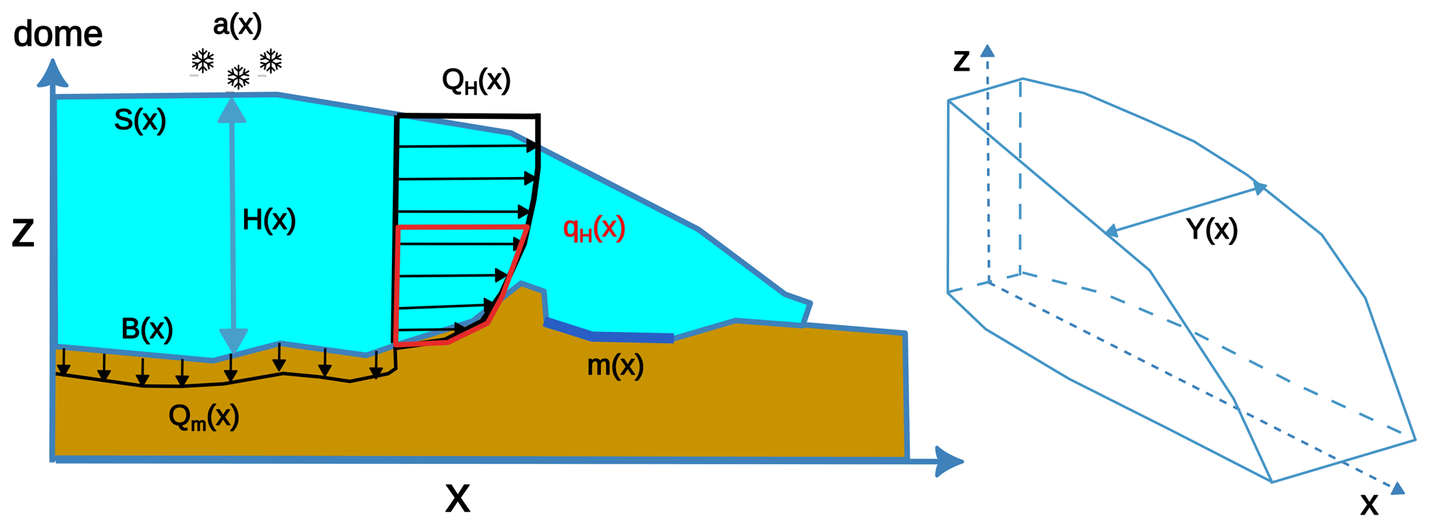
Figure 1 Diagram of the flow tube of an ice sheet with the principal notation used in this article.

We then define the horizontal and vertical velocity components in this new coordinate system: $u_{\mathit{\pi }}=\frac{\mathrm{d}\mathit{\pi }}{\mathrm{d}t}$ and $u_{\mathit{\theta }}=\frac{\mathrm{d}\mathit{\theta }}{\mathrm{d}t}$. Parrenin (2013) showed that these velocity components can be written as

$$\begin{array}{}\text{(9)}& \begin{array}{rl}& u_{\mathit{\pi }}={\displaystyle \frac{Y^{\mathrm{S}}a}{YD}}{\displaystyle \frac{\partial \mathrm{\Omega }}{\partial z}}\\ & u_{\mathit{\theta }}=-{\displaystyle \frac{Y^{\mathrm{S}}a}{YD}}{\displaystyle \frac{\partial \mathrm{\Omega }}{\partial z}}\end{array}\end{array}$$

where $Y^{\mathrm{S}}\left(x\right)=Y(x,S)$ is the tube width at surface. This way, it can immediately be seen (Parrenin and Hindmarsh, 2007), that these velocity components are equal in magnitude but opposite in sign. Therefore, trajectories in the (π, θ) coordinate system are straight lines of slope −1 (see Fig. 2).

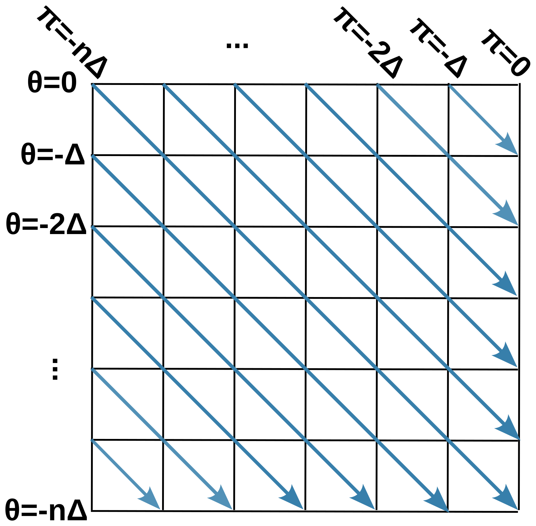
Figure 2 Diagram representing the (π, θ) grid (in black) and the trajectories (blue arrows) in this coordinate system.

Integrating the time spent along the trajectory from Eq. (9), the age of an ice particle can be written as

$$\begin{array}{}\text{(10)}& \mathit{\chi }=\underset{{\mathit{\pi }}_{\mathrm{0}}}{\overset{\mathit{\pi }}{\int }}\mathit{\kappa }\mathrm{d}\mathit{\pi }\end{array}$$

with π₀ the initial value of π when the ice particle was at surface and with the κ parameter defined as:

$$\begin{array}{}\text{(11)}& \mathit{\kappa }={\displaystyle \frac{YD}{Y^{\mathrm{S}}a}}{\displaystyle \frac{\partial z_{\mathrm{\Omega }}}{\partial \mathrm{\Omega }}}.\end{array}$$

We can now define the vertical thinning function, which is the ratio of the vertical thickness of a layer to its initial ice equivalent vertical thickness when it was at surface. Using this (π, θ) coordinate system, it can also be shown that the vertical thinning function can be written (Parrenin, 2013):

$$\begin{array}{}\text{(12)}& \mathit{\tau }=\mathrm{\Omega }{\displaystyle \frac{Y^{\mathrm{S}}a}{YD}}{\displaystyle \frac{D_{\mathrm{0}}}{a_{\mathrm{0}}}}{\left(\mathrm{1}-{\displaystyle \frac{\mathrm{1}}{\mathit{\kappa }}}\underset{{\mathit{\pi }}_{\mathrm{0}}}{\overset{\mathit{\pi }}{\int }}{\displaystyle \frac{\partial \mathit{\kappa }}{\partial \mathit{\pi }}}\right)}^{-\mathrm{1}}\end{array}$$

where D₀ and a₀ are respectively the relative density and accumulation rate when the snow/ice particle was deposited.

We can now consider variations of surface accumulation and basal melting rates and assume they have common temporal variations (Parrenin et al., 2006; Parrenin and Hindmarsh, 2007):

$$\begin{array}{}\text{(13)}& \begin{array}{rl}& a(x,t)=\stackrel{\mathrm{‾}}{a}\left(x\right)R\left(t\right)\\ & m(x,t)=\stackrel{\mathrm{‾}}{m}\left(x\right)R\left(t\right)\end{array}\end{array}$$

where $\stackrel{\mathrm{‾}}{a}\left(x\right)$ is the temporal average accumulation rate and $\stackrel{\mathrm{‾}}{m}\left(x\right)$ is the temporal average melting rate at position x. R(t) is a positive temporal multiplicative factor which can be determined from ice core data, e.g. using the relationship between the isotopic composition of ice and the surface accumulation rate. The implications of using the same temporal variation for basal melt rate and accumulation rate are discussed in Sect. 4.3. Using this assumption, the trajectories and isochrones are the same as those of the steady-state problem which uses $\stackrel{\mathrm{‾}}{a}$ and $\stackrel{\mathrm{‾}}{m}$, but velocities of ice particles are enhanced or reduced depending on the value of R(t). It is possible to deduce the real age of ice particles χ from the steady age $\stackrel{\mathrm{‾}}{\mathit{\chi }}$ using the following change of time variable

$$\begin{array}{}\text{(14)}& \stackrel{\mathrm{‾}}{t}=\underset{\mathrm{0}}{\overset{t}{\int }}R\left(t\right)\mathrm{d}t\end{array}$$

where $\stackrel{\mathrm{‾}}{t}$ is the steady time and t is the real time.

2.2 Simplifying assumptions

To simplify, we assume that snow is compressed instantaneously into ice at surface. In practice, we convert real depth into ice equivalent depth using a relative density profile informed by ice core observations or firn models in the simulated area. Moreover, we assume that the flow tube has vertical walls, that is, Y does not depend on z. This way, the equations for κ and τ become:

$$\begin{array}{}\text{(15)}& {\displaystyle }& {\displaystyle }\mathit{\kappa }={\displaystyle \frac{\mathrm{1}}{a}}{\displaystyle \frac{\partial z_{\mathrm{\Omega }}}{\partial \mathrm{\Omega }}}\text{(16)}& {\displaystyle }& {\displaystyle }\mathit{\tau }=\mathrm{\Omega }{\displaystyle \frac{a}{a_{\mathrm{0}}}}{\left(\mathrm{1}-{\displaystyle \frac{\mathrm{1}}{\mathit{\kappa }}}\underset{{\mathit{\pi }}_{\mathrm{0}}}{\overset{\mathit{\pi }}{\int }}{\displaystyle \frac{\partial \mathit{\kappa }}{\partial \mathit{\pi }}}\right)}^{-\mathrm{1}}.\end{array}$$

2.3 Numerical aspects

The (π, θ) coordinate system is very useful for solving any transport equation, a class to which the age equation belongs. Indeed, if we define a regular grid in (π, θ) with the same step $\mathrm{\Delta }\mathit{\pi }=\mathrm{\Delta }\mathit{\theta }=\mathrm{\Delta }$, the trajectories of ice particles pass exactly through the nodes of the grid (Fig. 2). Therefore, starting from the surface where the age is χ=0, it is possible to deduce the age on the horizontal grid line below where $\mathit{\theta }=-\mathrm{\Delta }$ by calculating the time needed for each ice particle to cross a cell. Then the age on the horizontal grid line below ($\mathit{\theta }=-\mathrm{2}\mathrm{\Delta }$) can be calculated, etc. As particles move downstream, the conditions at the upstream boundary should be known. As the π scale is logarithmic, there is a singularity at the dome. Therefore, the horizontal π scale starts at a point slightly downstream of the dome, where an age can be prescribed, for example using a dome solution (which assumes purely vertical movement). If one is interested in a flank ice core, the upstream boundary can be chosen such that the upstream condition does not affect the age modelling of the ice core, i.e., the ice in the ice core comes from the surface boundary and not from the upstream boundary.

The time needed to cross a cell is

$$\begin{array}{}\text{(17)}& \mathrm{\Delta }\mathit{\chi }=\underset{\mathit{\pi }}{\overset{\mathit{\pi }+\mathrm{\Delta }}{\int }}\mathit{\kappa }\mathrm{d}\mathit{\pi }.\end{array}$$

Here, we assume that $\mathrm{1}/a$ is continuous and varies linearly between two consecutive π nodes. Similarly, we assume that z_Ω is continuous and varies linearly between two consecutive θ nodes along a vertical grid line (Fig. 2). It means that $\frac{\partial z_{\mathrm{\Omega }}}{\partial \mathrm{\Omega }}$ is a stepwise function along θ and a continuous and linear-by-parts function along π. Integrating κ along π across a cell therefore corresponds to integrating a second order polynomial.

Similarly, we can calculate the vertical thinning function using Eq. (11) by integrating the following quantity along each cell:

$$\begin{array}{}\text{(18)}& \underset{\mathit{\pi }}{\overset{\mathit{\pi }+\mathrm{\Delta }}{\int }}{\displaystyle \frac{\partial \mathit{\kappa }}{\partial \mathit{\pi }}}\mathrm{d}\mathit{\pi }\end{array}$$

with our assumption that $\mathrm{1}/a$ and z_Ω are piecewise linear functions, $\partial \mathit{\kappa }/\partial \mathit{\pi }$ is a first order polynomial between π and π+Δ, so it can be easily integrated.

To calculate the initial horizontal positions, the total flux or the initial accumulation rate when the ice particles were at surface, we must transport these quantities from the surface along the diagonals in the (π, θ) grid (Fig. 2). The trajectories of the particles are given by the iso-contours of the stream function q.

In our age_flow_line-1.0 code, it is possible to determine the age, accumulation and thinning function on a refined vertical grid corresponding to an existing or potential ice core. We first determine the π coordinate of the ice core and calculate the age and thinning profiles by a weighted average of the two adjacent vertical profiles of the 2D grid. We then interpolate this coarse 1D vertical profile onto a refined 1D ice core profile. For the thinning function, we perform a linear interpolation while, for the age, we use a quadratic interpolation.

In order to verify that the uncertainty due to interpolation is negligible, we also use a different method to estimate the thinning function and age at the ice core location. Once the age, thinning and the initial accumulation rate are calculated for an ice core, we derive the age to get another estimate of the thinning function, and we integrate the layer thickness to get another estimate of the age. We then check that the two estimates of age and thinning (one integrating the age and the other integrating the thinning) are consistent within numerical uncertainties.

2.4 Programming aspects

age_flow_line-1.0 is entirely written using the Python-3 programming language with several scientific modules as dependencies (numpy, scipy, matplotlib). age_flow_line-1.0 both solves the transport equations and displays the results as figures. The figures displayed for the 2D grid are: the 2D grid in the (x, z) and (π, θ) coordinate system, the age in the x, z), (x, d) and (π, θ) coordinate systems, thinning in the (x, z) coordinate system, obtained either by direct integration of the thinning or by differentiation of the age, the ω function in the (x, z) coordinate system, the stream function q and its contours (the stream lines, which represent particle trajectories) in the (x, z) coordinate system. Along the x coordinate of the flow line, figures display the accumulation rate, the basal melting rate, the width of the flow tube and the surface velocity or the total flux Q. Along the 1D vertical grid of each ice core, one figure displays the accumulation and layer thickness as a function of the age, and another figure displays the age, spatial origin and thinning as a function of depth.

For the horizontal flux shape function ω, we use the Lliboutry profile (Lliboutry, 1979; Parrenin and Hindmarsh, 2007):

$$\begin{array}{}\text{(19)}& \mathit{\omega }\left(\mathit{\zeta }\right)=\mathrm{1}-{\displaystyle \frac{p+\mathrm{2}}{p+\mathrm{1}}}(\mathrm{1}-\mathit{\zeta })+{\displaystyle \frac{\mathrm{1}}{p+\mathrm{1}}}(\mathrm{1}-\mathit{\zeta }{)}^{p+\mathrm{2}}\end{array}$$

where ζ is the normalised vertical coordinate (0 at the bedrock and 1 at the surface). Therefore, only the value of p needs to be defined for each horizontal position x along the flow line. However, one could easily implement another type of horizontal flux shape function, for example the Dansgaard–Johnsen profile (Johnsen and Dansgaard, 1992).

For the upstream boundary condition on the age, we impose a dome profile:

$$\begin{array}{}\text{(20)}& \mathit{\chi }=\underset{\mathit{\theta }}{\overset{\mathrm{0}}{\int }}\mathit{\kappa }\mathrm{d}\mathit{\theta }.\end{array}$$

The core of the code is entirely separate from the experiment directory where the results of the run are saved. The experiment directory is composed of a general parameter file in the YAML format (age_flow_line-1.0 uses the pyaml module) and text files that define the accumulation rate a, basal melting rate m, width of the flow tube Y, surface elevation S, ice sheet thickness H and exponent of the Lliboutry profile p. There is also a vertical density profile given in a text file for transforming real depths to ice equivalent depths and this profile is assumed to be the same along the whole flow line.

3 Application to the DC-BELDC flow line

To demonstrate the performance and ability of our age model, we apply it to the East Antarctica flow line between DC and the BELDC drill site. Beyond EPICA is a European project that aims to drill a continuous ice core record back to 1.2 million years at least, which makes this flow line particularly interesting. Numerical modelling is necessary to estimate the age of the ice deeper than the deepest visible radar horizons and to estimate the trajectories of ice particles. The DC-BELDC flow tube has already been determined in the companion paper by Chung et al. (2025). It is ∼40 km long with a strong lateral flow divergence because the proposed coring site is on a divide (Fig. 3). The parameters used for our simulations, namely the surface accumulation rate, basal melting and Lliboutry parameter, are those from Chung et al. (2023) obtained by fitting a 1D pseudo-steady age model onto observed isochrones. This 1D model finds a best fit value for a mechanical ice thickness and uses the comparison with the observed ice thickness to infer basal conditions. For consistency and the sake of comparison, it is therefore the mechanical ice thickness that we use for our bottom boundary condition here, instead of the observed ice thickness. The aim of our simulation here is to estimate whether horizontal advection is an important mechanism to take into account in the modelling of the age along this flow line, by comparing the result of 1D and 2.5D models with the same set of parameters. This 2.5D simulation is however not fully optimized. This is because we are using the results of the 1D inverse model for a 2.5D flow tube model, instead of optimizing the 2.5D model directly onto the observed isochrones and ice core datasets. The optimization of this 2.5D model is the scope of the companion paper by Chung et al. (2025).

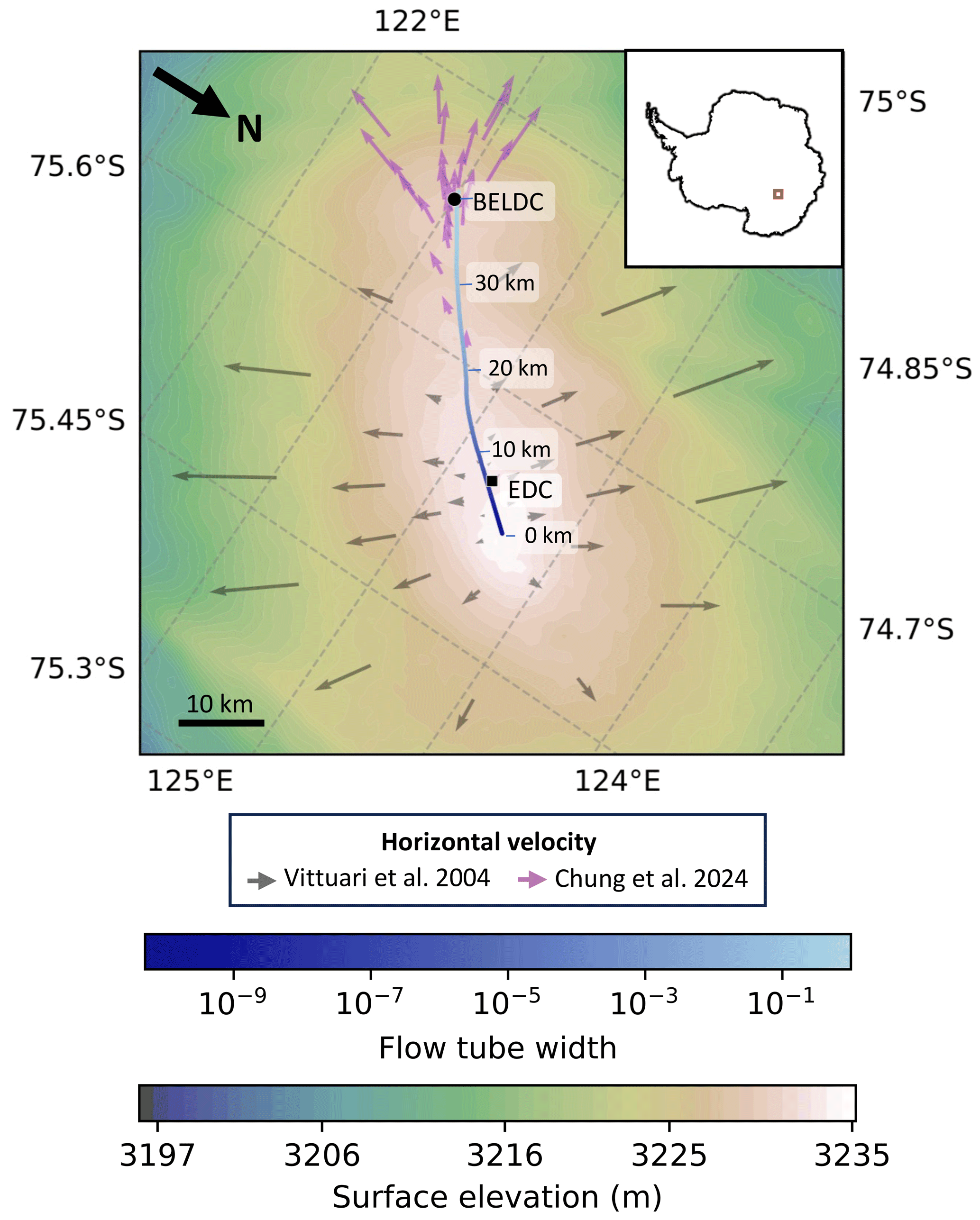
Figure 3 Map of the flow line (central blue line) going from DC to BELDC with the width of the flow tube according to the blue colour bar. The background colour represents the surface elevation. The grey and pink arrows represent surface velocity measurements. Adapted from Chung et al. (2025).

The boundary conditions of the model are plotted in Fig. 4. The accumulation and basal melting rates are taken from the 1D inverse model (Chung et al., 2023), while the flow tube width is calculated from the back-tracking of adjacents flow lines from BELDC (Chung et al., 2025). The meshes of the model are plotted in Fig. 5. The horizontal flux shape function ω is plotted in Fig. 6. The modelled age, trajectories and vertical thinning function are plotted in Figs. 7–9. The results for the next ice core at BELDC are plotted in Fig. 10. These figures (from 4 to 10) are automatically generated by the age_flow_line-1.0 software.

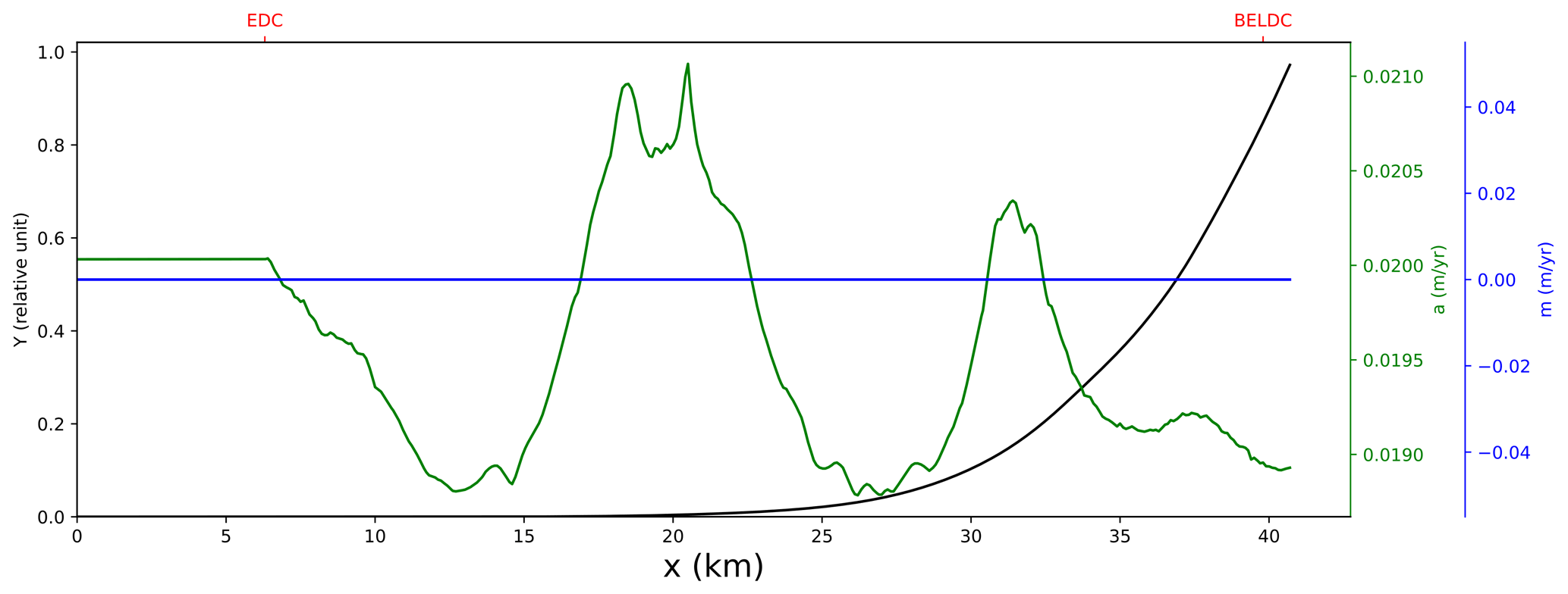
Figure 4 Boundary conditions of the model along the DC-BELDC flow line: surface accumulation rate (green), basal melt rate (blue) and tube width (black). Note that basal melting rate is zero, as a consequence of using a mechanical ice thickness. The position of the EDC and BELDC drilling sites are indicated in red on the top bar. This figure was automatically generated by the age_flow_line-1.0 software.

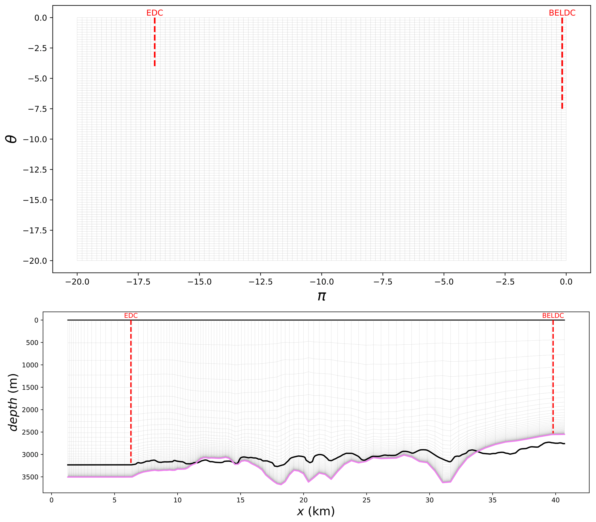
Figure 5 Mesh of the age_flow_line-1.0 model experiment in the (π, θ) (top panel) and (x, z) (bottom panel) coordinate system. The positions of the EDC and BELDC deep drill sites are plotted in dashed red. The observed bedrock is in thick black and the mechanical bedrock in violet. For better readability, the resolution of the grids has been decreased by a factor of 10. Note that in the top panel, the EDC and BELDC ice cores do not extend down to the bottom of the mesh, since this mesh converges asymptotically towards the mechanical bedrock but never reaches it. These figures were automatically generated by the age_flow_line-1.0 software.

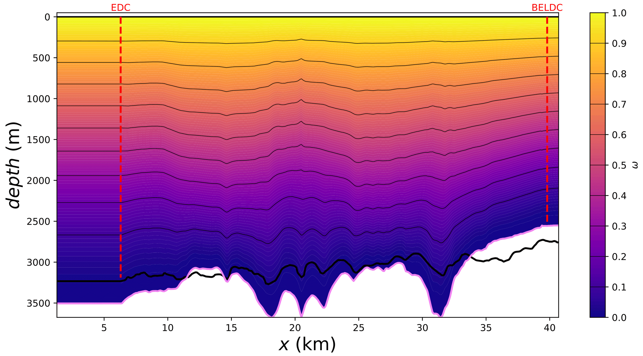
Figure 6 The ω horizontal flux shape function along the DC-BELDC flow line. The positions of the EDC and BELDC deep drill sites are plotted in dashed red. The observed bedrock is in thick black and the mechanical bedrock (the elevation where the extrapolated velocity becomes zero) in violet. This figure was automatically generated by the age_flow_line-1.0 software.

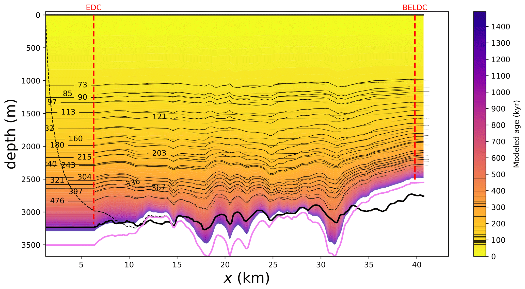
Figure 7 Modelled age along the DC-BELDC flow line, according to the colour scale on the right. The modelled isochrones are plotted in solid black and their age is represented on the colour bar. The positions of the EDC and BELDC deep drill sites are plotted in dashed red. The black dashed line represents the trajectory originating from the surface upstream corner. The dotted black lines are the isochrones observed by radar. The observed bedrock is in thick black and the mechanical bedrock in violet. This figure was automatically generated by the age_flow_line-1.0 software.

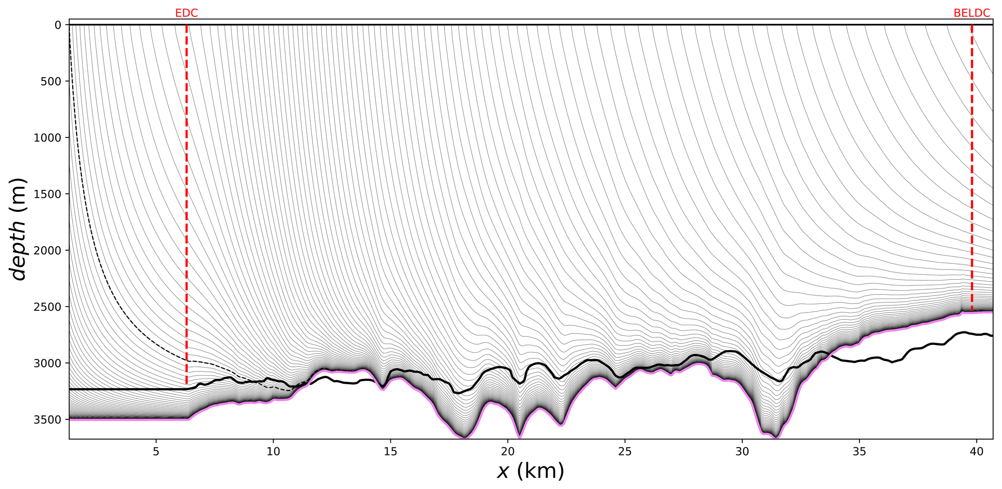
Figure 8 Trajectories of ice particles (black lines) along the DC-BELDC flow line which is situated along a divide. The positions of the EDC and BELDC deep drill sites are plotted in dashed red. The black dashed line represents the trajectory originating from the surface upstream corner. The observed bedrock is in thick black and the mechanical bedrock in violet. This figure was automatically generated by the age_flow_line-1.0 software.

Figure 9 Value of the vertical thinning function along the DC-BELDC flow line. The two vertical red dashed lines represent the positions of the EDC and BELDC drill sites. The black dashed line represents the trajectory originating from the surface upstream corner. The observed bedrock is in thick black and the mechanical bedrock in violet. The thinning functions for EDC and BELDC are shown in Fig. 10. This figure was automatically generated by the age_flow_line-1.0 software.

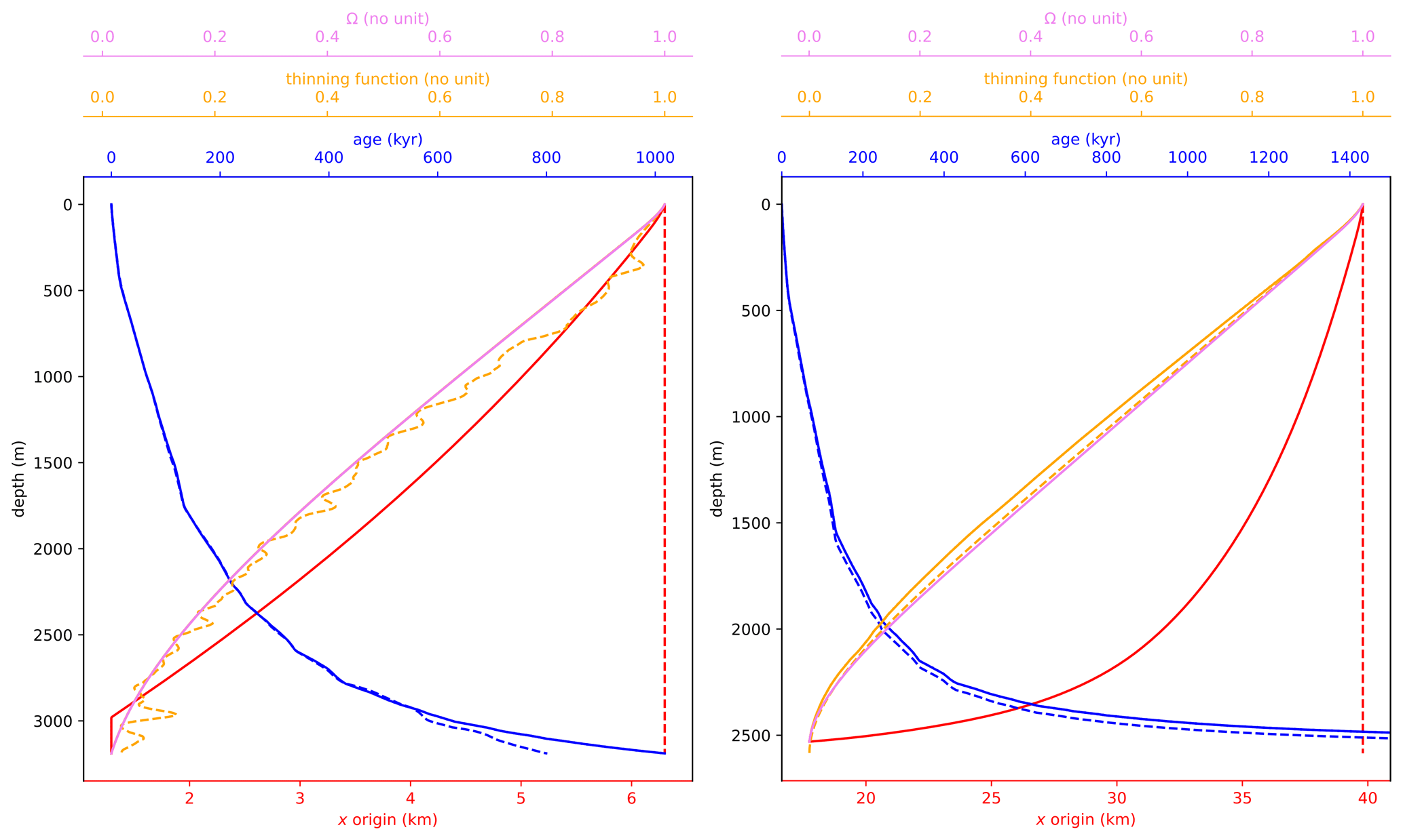
Figure 10 Age (blue), vertical thinning function (orange), Ω flux shape function (violet) and spatial origin (red) of the ice at the EDC (left panel) and BELDC (right panel) drill site locations. The solid lines represent the 2.5D age_flow_line-1.0 results. The dashed lines represent the AICC2012 chronology for EDC and the results of the 1D model (Chung et al., 2023) for BELDC. Note that for EDC, the orange and violet solid lines are superimposed. These figures were automatically generated by the age_flow_line-1.0 software.

Figure 5 shows that the mesh is refined near the ice-bedrock interface. This is expected, since the grid is exponential with respect to the flux shape function Ω. When there is no basal melting (which is the case in our application with the mechanical ice thickness), the grid does not extend down to the bedrock but approaches it asymptotically. The horizontal resolution also varies in our application, but several parameters affect this resolution. One would expect the horizontal resolution to decrease when the distance to the dome increases, since the grid is exponential in total flux Q. But this is partially compensated by the exponential increase of the tube width along the flow line.

Figure 8 shows that the ice particles may originate >15 km upstream along the divide. Therefore, horizontal flow is not negligible along this flow line and should be taken into account when modelling the age of the ice. In particular at BELDC (Fig. 10), the bottom ice originates up to ∼22 km upstream from the drilling site.

4 Discussion

4.1 Numerical aspects

This age model is accurate and exhibits minimal numerical diffusion since quantities are transported from one node to the next without interpolation. This could help test the accuracy of numerical schemes of more complex 3D and transient models.

This model has similar complexity of a steady-state model but considers the variations of accumulation with time which is non-negligible along a glacial-interglacial cycle (approximately a factor of 2 on the East Antarctic plateau). For a 1000×1000 grid, the computation time is ∼0.1 s on a recent laptop computer for the numerical calculations, with a few additional seconds for the building of the figures. For this grid, the memory footprint of the simulation is ∼0.8 GB.

Due to its fast computation time, this model is appropriate for inverse simulations where the results are fitted to observations. Indeed, inverse simulations require multiple runs of the forward model to find the optimal set of parameters, which can be computationally expensive.

This model could also be appropriate for representing the advection term in a heat equation, although the diffusion term is better dealt with in a physical (x, z) coordinate system.

4.2 Modelling of the DC-BELDC flow line

We have performed a simulation where both vertical and horizontal ice flows are taken into account. We show that horizontal flow has a non negligible effect on the age modelling of the BELDC ice core, since our modelled isochrones do not have the same geometry than the ones simulated by the 1D model (Chung et al., 2023) when using the same set of input parameters. Indeed, while the 1D model simulates isochrones very close to the observed ones (Chung et al., 2023), the isochrones simulated by the 2.5D model significantly deviate from them (Fig. 7), with deviations of >100 m at some places. In our forward simulation using parameters inverted by the 1D model, particles originate sometimes >15 km from their current position. Our simulation is provided as a proof of concept for the model we have developed. However, it is not appropriate to use the result of the 1D inverse model by Chung et al. (2023) to determine the parameters of the 2.5D model. For a more realistic simulation, the parameters of the model should be optimized so that modelled age fits the radar and ice core age observations. This is the purpose of the companion paper of Chung et al. (2025) who developed this inverse methodology.

4.3 Limitations of the pseudo-steady assumption

Our model relies on the pseudo-steady assumption, which states that all variables are in steady-state except for a temporal multiplicative factor which is both applied to accumulation and melting.

First, the geometry is assumed to be in steady-state. This assumption is adapted for the interior of East Antarctica, where relative variations in ice thickness were small (Ritz et al., 2001), but it still requires that the flow lines have not varied too much in the past, which is still unclear. Greenland and West Antarctica have probably encountered more important changes since they are more sensitive to climatic variations in the ocean and in the atmosphere (Quiquet et al., 2013; Wolff et al., 2025).

Second, the same temporal multiplicative factor is applied to both surface accumulation and basal melting. There are no physical reason to assume surface accumulation and basal melting have varied in concert; this is just a mathematical convenience. However, in regions where basal melt rates are low, this assumption should not introduce major errors, as long as a realistic time-averaged basal melt rate is prescribed. Moreover, this temporal factor assumes that the surface accumulation spatial pattern has remained stable in time. This assumption relies on a stable snow precipitation process and a stable snow re-deposition by wind, which might not always be the case (Cavitte et al., 2018).

Our pseudo-steady model can therefore be seen as a first approach to model the age field along flow lines at high resolution, but more complex 3D and transient models are necessary to fully investigate the age of the ice in ice sheets.

4.4 Possible improvements

In this implementation, we have made a few simplifying assumptions that could be relaxed in the future. First we assumed that the flow tube has vertical walls, which is for example not the case along a ridge (Passalacqua et al., 2016). Second, we converted real depths into ice equivalent depth using a unique density profile along the flow line, while clearly for long flow lines the density profile might change with the distance from the dome. Third, we used a Lliboutry profile for the horizontal flux shape function ω, while other profiles could be used. In particular at a steady-state dome where Raymond arches develop (Raymond, 1983), the Lliboutry profile does not seem to be suitable (Martín and Gudmundsson, 2012). Fourth, we prescribed a dome solution on the upstream boundary of the domain, but any boundary condition could be prescribed.

Due to the numerical simplicity of the model, it may be possible to derive its Jacobian, which would make inverse simulations more efficient.

4.5 Possible applications and comparison with other modelling efforts

The value of this model lies in its high numerical accuracy and very fast computation time. It is appropriate for long flow lines, old age and for parameter inferences. The companion paper of Chung et al. (2025) outlines its interest, since we can optimize its parameters in a couple of minutes on a personal computer. However, this model has physical assumptions which might introduce errors. To overcome this limitation, our model could be used in conjunction with a transient model like the one developed by Buchardt and Dahl-Jensen (2007) or Gerber et al. (2021). For example, our model could provide an initial condition which could be refined using the transient model. It could also provide a “first guess” and a fast approximation of the Jacobian of the transient model, to speed up the optimization of its parameters.

This flow tube model could be applied to several nearly steady-state flow lines of the current Greenland and Antarctic ice sheets, especially those that have ice core information.

The Vostok flow line in East Antarctica was originally modelled by Ritz (1992) but only the age along the Vostok ice core was calculated by a Lagrangian tracer scheme. This work was later extended by Parrenin et al. (2001, 2004) who optimized some parameters of the model to fit the ice core age observations, but still without accounting for the isochronal information. Another flow tube model was developed and applied to the Vostok flow line by Salamatin et al. (2009), accounting for both the ice core and isochronal age observations. It would be valuable to apply the current numerical model to this Vostok flow line and compare the results with these previous modelling efforts.

The EDML ice core in East Antarctica is situated on a ridge and horizontal flow also needs to be taken into account. Huybrechts et al. (2007) applied a large scale ice sheet model of Antarctica with a local high resolution and high order model nested inside around EDML. It would be valuable to see how our numerical model, with its very high resolution and numerical accuracy and its fitting to isochronal observations, compares with this previous transient and large scale model.

The NEEM and NorthGRIP ice cores in Greenland are also situated on a ridge coming from Summit. Isochrones around NorthGRIP were simulated using a flow tube model by Buchardt and Dahl-Jensen (2007) and fitted to radar observations. The basal melting was hence deduced. Applying our numerical model to this flow line, we could compare it to the previous work and see if its high resolution and accuracy can improve the modelling scenario.

Another interesting flow line in Greenland is the one going from Summit to the EastGRIP ice core. The age of the ice along this profile was modelled by Gerber et al. (2021) using a similar model to that of the NorthGRIP flow line, based on a Dansgaard–Johnsen velocity profile (Johnsen and Dansgaard, 1992). Again, our numerical model could be compared to this previous modelling effort.

5 Conclusions

For the interpretation of radar-observed isochrones or ice core chronologies, it is sometimes necessary to simulate the age of the ice in an ice sheet. We have developed a numerical model to calculate the age of the ice along a pseudo-steady flow tube of an ice sheet. Our Eulerian-Lagrangian scheme combines advantages of Eulerian and Lagragian schemes. There is a regular grid where the age is calculated, as in Eulerian schemes, which is significantly more convenient than having to define initial particle positions and tracking these positions during the time evolution. But at the same time, there is no numerical diffusion, as in Lagrangian schemes, and our model is numerically very accurate. Our model is computationally effective, opening up new prospects for optimizing its parameters according to observations, which requires many forward simulations runs. We have applied our model to the DC-BELDC flow line and we have shown that horizontal flow is non negligible there, with ice particles sometimes travelling >15 km which has implications for the age scale of the BELDC ice core. The next step is to optimize the parameters of the model according to age observations such as radar-observed isochrones and ice core dated horizons, which is done in the companion manuscript (Chung et al., 2025).