Urban weather modeling using WRF: linking physical assumptions, code implementation, and observational needs

The Weather Research and Forecasting (WRF) model includes urban schemes that simulate the influence of urban surfaces on the atmosphere using parameterizations for flux, and radiative exchanges. Three core schemes – the Bulk urban parameterization, Single-Layer Urban Canopy Model (SLUCM), and Multi-Layer Urban Canopy Model (MLUCM) – represent increasing levels of complexity. Although the parameterizations within these urban schemes are described in the literature, their specific implementation remains poorly documented, thus slowing down model development efforts.

This manuscript provides a roadmap to the three urban schemes in WRF version 4.5.2, presenting equations using the same symbols as in the model code, along with references to code lines, and including graphics and explanations that connect the code to its physical foundations. Our thorough review of the urban parameterizations implemented in WRF version 4.5.2 highlighted a handful of parameters that may introduce discontinuities in simulations: (i) in the SLUCM, a 1 mm h⁻¹ rain rate threshold is employed to switch between two minimum moisture availability parameterizations, thus impacting latent heat flux calculations; (ii) in the SLUCM a threshold is used to partition shortwave radiation into direct and diffuse components; (iii) in all three urban schemes, the bulk Richardson number is employed to select the similarity function, which influences the vertical distribution of heat and momentum. We also identified a highly simplified treatment of the radiative balance on roof surfaces. The implications of these simplifications can be assessed through targeted observations across relevant conditions, including varying precipitation rates, cloud cover, and transitions between stability regimes. Furthermore, the widespread application of the Monin-Obukhov similarity theory in these urban schemes warrants model evaluation under highly stable and unstable conditions and in heterogeneous urban settings with variable land cover and building heights on scales finer than model resolution. To address these challenges, we offer guidance on observational strategies, emphasizing the need for multi-parametric measurements to capture potential compensating biases and multi-height measurements that align with the levels where quantities are diagnostic and prognosed in the model (i.e., the lowest atmospheric level of the WRF model). Finally, our inspection of the code revealed implementation bugs that have now been corrected in WRF versions 4.6.0 and 4.6.1. Sensitivity tests over the Atlanta urban area show that these corrections affect surface temperatures, underscoring the importance of performing rigorous documentation and verification of the implementation of parameterizations in model code.

1 Introduction

Weather Research and Forecasting (WRF) is a mesoscale atmospheric model widely used for research and short- to medium-range weather forecasting (Lynn and Yair, 2010) as well as regional long-term climate simulations (Rasmussen et al., 2023). Over the past decade, development efforts have expanded the capabilities of the WRF model (Powers et al., 2017) to include, among other things, chemistry (WRF-Chem; Grell et al., 2005), hydrology (WRF-Hydro; Gochis et al., 2015), and urban processes (WRF-Urban; Chen et al., 2011).

Urban environments, now home to more than half of the global population (United Nations, 2015), introduce significant heterogeneity in surface energy exchange due to impervious materials, complex geometries, and anthropogenic heat emissions. These complexities modify the atmospheric structure, especially in the lowest kilometer of the boundary layer (Lee et al., 2011), and require specialized modeling approaches. The community version of WRF includes three urban schemes – the Bulk scheme (also know as the Slab model), the Single-Layer Urban Canopy Model (SLUCM), and the Multi-Layer Urban Canopy Model (MLUCM) – that represent urban processes with varying levels of complexity. Despite their widespread use in urban climate research (e.g., Georgescu et al., 2024; Zhu and Ooka, 2023), the numerical implementations of these schemes are poorly documented, limiting model development, and lacking transparency regarding parameter manipulations needed to integrate urban parameterizations with other WRF modules. Improved documentation would help identify key parameters that influence model performance and guide targeted observations, better aligning modeling efforts with measurement strategies to enhance predictability.

This work seeks to complement the literature focused on the underlying physics of urban parameterizations in the WRF-Urban (e.g., Garuma, 2018; Tarasova et al., 2023; Grimmond et al., 2010; Masson, 2006; Barlow, 2014). It sets itself apart by providing a detailed roadmap of the parameterizations employed in WRF-Urban as implemented in the model version 4.5.2 using the exact mathematical symbols employed in the model code and referencing the code line numbers to accelerate future efforts to develop the code. We also provide new graphical schematics to guide the reader through the relevant physical concepts to improve users understanding of key model assumptions. We identified a handful of parameters that may introduce discontinuities in simulations, for which we offer guidance on strategies to assess their impact and/or tune them with observations. Additionally, our systematic code review uncovered several implementation bugs, which we document here. Sensitivity simulations are presented to illustrate the potential impact of these bugs on model output, emphasizing the importance of continued model code verification.

2 WRF-Urban modeling system

2.1 General description of the WRF urban canopy models

The WRF-Urban code package contains three schemes to simulate the effects of urban surfaces and on turbulent fluxes and radiation: the Bulk urban parameterization, the SLUCM, and the MLUCM, which includes the Building Effect Parameterization (BEP) model, which is often coupled with the Building Energy Model (BEM).

The Bulk urban parameterization, originally presented in (Chen et al., 2011; Liu et al., 2006), simplifies urban areas by representing them as one flat, uniform surface with adjusted physical properties. These adjustments include increased heat capacity, thermal conductivity, and surface roughness, along with reduced albedo. This simplified framework makes the Bulk urban Parameterization computationally efficient and well suited for studies where high-resolution urban details are unnecessary or where data availability and computational resources are constrained.

The WRF-Urban urban canopy models (UCMs) – the SLUCM (Kusaka et al., 2001) and the BEP (Martilli et al., 2002) – provide more detailed representations by simulating urban environments as idealized canyons. The SLUCM and BEP have several surface types, each of which is treated independently, with separate calculations for turbulent and radiative processes. Both the SLUCM and BEP models can represent a mix of roof types, such as green roofs and traditional roofs, within the same grid cell. However, they are limited to representing a single type of wall and street per grid cell. The primary distinction between SLUCM and BEP lies in their vertical structure. The SLUCM represents buildings as an infinitely long 2D array of buildings of uniform height, and simulates the urban canopy as a single homogeneous layer beneath the first atmospheric layer (Hang et al., 2024). In contrast, the BEP model resolves the urban canopy layer into multiple vertical levels, which extend within but do not necessarily align with the atmospheric levels in the WRF model. Building heights are represented as a distribution function and, at each level, energy balance equations are solved taking into account the probability that buildings are equal to or exceeding that height. This approach allows BEP to provide a more detailed and realistic representation of interactions within and above urban canyons. However, the added complexity comes at the cost of higher computational demands compared to single-layer models (Garuma, 2018). When coupled with the BEM model, BEP-BEM extends the dimensions of the BEP urban modeling framework by simulating, among other things, latent heat fluxes, windows on walls, building energy use, and anthropogenic heat emissions (Salamanca and Martilli, 2010). A single grid cell in a mesoscale model typically contains numerous buildings and streets that vary in physical characteristics such as height, width, and thermal properties. However, representing these heterogeneous features with a single, uniform type of building or street oversimplifies the complexity of real urban morphology. Therefore, a more realistic depiction of urban areas requires advanced urban canopy models that incorporate multiple types of buildings and their distinct thermal attributes.

Fundamentally, each of these urban models prognoses the surface temperature T for each represented surface (e.g., roof, wall, and road) as well as turbulent fluxes (sensible heat SH and latent heat LH) between these urban surfaces and the ambient air. The parameters enter the energy balance calculation for each represented surface alongside the net radiation R_net, and the ground heat flux G:

$$\begin{array}{}\text{(1)}& C_p{\displaystyle \frac{\partial \left(T\right)}{\partial t}}=R_{\mathrm{net}}-G-\mathrm{SH}-\mathrm{LH},\end{array}$$

where

$$\begin{array}{}\text{(2)}& R_{\mathrm{net}}=\mathrm{SW}+\mathit{ϵ}\left(\mathrm{LW}-{\mathrm{UP}}_{\mathrm{flux}}\right),\end{array}$$

where C_p is the heat capacity of the surface per unit area, SW is the downward SWR flux absorbed by the surface, LW is the total downward longwave radiative heat flux, UP_flux is the outgoing LW radiative flux, and ϵ is the emissivity of the surface under consideration. Given their varying levels of complexity, each urban model in WRF employs distinct parameterization formulations and assumptions to compute fluxes. The following subsections delve into these differing approaches.

3 Turbulent fluxes

3.1 Sensible heat flux parameterizations

3.1.1 BOX 1 – underbraces under equations to inform the reader as to the location of the equation in the WRF v4.5.2 code

For example, Eq. (3) for HFX is implemented on line 409 of file module_sf_slab.F in WRF v4.5.2.

Despite differences in the way they represent urban surfaces, the Bulk , SLUCM, and BEP parameterizations for sensible heat flux share several fundamental similarities. All employ a bulk aerodynamic formulation that depends on (i) the temperature gradient between the represented surface(s) and the adjacent air, (ii) wind speed, and (iii) heat/moisture transfer coefficients, which incorporate atmospheric stability effects through the Bulk Richardson number. Additionally, all rely on the Monin–Obukhov Similarity Theory (MOST) to estimate surface fluxes.

In the Bulk model, sensible heat flux is estimated based on the potential temperature difference between the slab surface (THG) and the temperature of the air at the first atmospheric level (THX), as well as the heat transfer coefficient of the air (FLHC) following the formulation of Zhang and Anthes (1982):

$$\begin{array}{}\text{(3)}& \underset{\begin{array}{c}\mathrm{Line}\mathrm{410},\\ \mathrm{module}\mathrm{\_}\mathrm{sf}\mathrm{\_}\mathrm{slab}.\mathrm{F}\end{array}}{\underbrace{\mathrm{HFX}}}=\mathrm{FLHC}\times (\mathrm{THG}-\mathrm{THX}).\end{array}$$

(FLHC) takes into account the specific heat of dry air at constant pressure CPM, the air density RHOX, and the potential temperature of the slab surface THGB as well as the turbulent velocity scale UST and the temperature scale MOL following:

$$\begin{array}{}\text{(4)}& \begin{array}{rl}\underset{\begin{array}{c}\mathrm{Line}\mathrm{877}\\ \mathrm{module}\mathrm{\_}\mathrm{sf}\mathrm{\_}\mathrm{sfclay}.\mathrm{F}\end{array}}{\underbrace{\mathrm{FLHC}}}=& \mathrm{CPM}\times \mathrm{RHOX}\times \mathrm{UST}\times \mathrm{MOL}/\\ & (\mathrm{THX}-\mathrm{THGB}).\end{array}\end{array}$$

The temperature scale MOL incorporates the potential temperature difference between the ground and the lowest atmospheric model level (DTG) and the integrated similarity function for heat PSIT following

$$\begin{array}{}\text{(5)}& {\displaystyle }& {\displaystyle }\underset{\begin{array}{c}\mathrm{Line}\mathrm{815}\\ \mathrm{module}\mathrm{\_}\mathrm{sf}\mathrm{\_}\mathrm{sfclay}.\mathrm{F}\end{array}}{\underbrace{\mathrm{MOL}}}={\displaystyle \frac{\mathrm{KARMAN}\cdot \mathrm{DTG}}{\mathrm{PSIT}\cdot \mathrm{PRT}}},\text{(6)}& {\displaystyle }& {\displaystyle }\mathrm{DGT}=(\mathrm{THX}-\mathrm{THGB})\end{array}$$

where KARMAN is the von Karman constant and PRT is the Prandtl number with a constant value of 1.

The friction velocity UST incorporates the wind speed at the lowest atmospheric level (WSPD) and the integrated similarity function for momentum PSIX, following:

$$\begin{array}{}\text{(7)}& \underset{\begin{array}{c}\mathrm{Line}\mathrm{794}\\ \mathrm{module}\mathrm{\_}\mathrm{sf}\mathrm{\_}\mathrm{sfclay}.\mathrm{F}\end{array}}{\underbrace{\mathrm{UST}}}={\displaystyle \frac{\mathrm{KARMAN}\cdot \mathrm{WSPD}}{\mathrm{PSIX}}}.\end{array}$$

Under strongly unstable conditions, additional corrections can be applied to WSPD to account for convective velocity scaling following Beljaars (1995) and subgrid-scale turbulence effects following Mahrt and Sun (1995).

The integrated similarity functions PSIT and PSIX were derived empirically using the MOST formulation (Beljaars and Holtslag, 1991), which also allows for the derivation of vertical profiles of meteorological variables, enabling the diagnostic estimation of quantities such as 2 m air temperature and 10 m wind speed at standard observational heights (see Box 2). In the Bulk scheme, the bulk Richardson number is used to select among four different integrated similarity formulations (Jiménez et al., 2012). However, this reliance on bulk Richardson number thresholds to choose the appropriate integrated similarity functions introduces discontinuities and inconsistencies in flux calculations, particularly in transition regimes. Observational data could help inform the use of this parameter. Further discussion of this topic will be provided in Sect. 3.3.

Among the similarity function formulations implemented in the Bulk scheme are those of Fairall et al. (1996) for neutral to free convective conditions, and Chenge and Brutsaert (2005) for neutral to very stable conditions. These formulations extend the original similarity functions derived from the Kansas field program using a limited number of observations over flat, homogeneous surfaces (Izumi and Barad, 1970; Businger et al., 1971; Dyer, 1974; Hicks, 1976). Given the complexity and heterogeneity of urban environments, additional observational datasets that cover a wider range of urban settings could help refine these empirical similarity functions. A discussion of observational approaches for improving these formulations is provided in Sect. 3.3.

The integrated similarity functions (PSIT and PSIX) are corrected for the excess aerodynamic resistance of urban areas following the proposed approach (Chen and Zhang, 2009). This effectively diminishes the efficiency of turbulent transfer in urban areas. This is achieved by adopting a modified formulation of the roughness length for heat, which takes into account the Reynolds number and the Zilitinkevich coefficient (Czil) – an empirical coefficient for bulk transfer. In the WRF version 4.5.2, Czil is set to 0.1. Chen et al. (1997) and Chen and Zhang (2009) designed a calibration procedure for Czil which relies on the comparison of observed and simulated fluxes collected over different land-cover type. They also present an empirical formula for Czil, which relates it to canopy height (Eq. 4 in Chen and Zhang, 2009). The same procedure could be repeated over other urban environments to further tune Czil.

In the SLUCM a distinction is made during the sensible heat flux calculation for each surface (H_[surface]) to account for the fact that the roof surfaces are closer to the first atmospheric level, than building walls and ground. This distinction leads to using different air temperature and wind information when calculating heat flux for the roof (R) and green roof (GR) surfaces (Eq. S1 in the Supplement) compared to the wall (B) and ground (G) surfaces (Eq. 8). Where canopy wind speed UC is used for the building walls and ground surfaces, wind speed at the lowest atmospheric level, denoted as UA, is used for the roof surfaces. Similarly, where the canopy temperature TCP is used for building walls and ground calculations, the air temperature at the lowest atmospheric level of the WRF mesoscale model TA is employed for roof surface calculations.

$$\begin{array}{}\text{(8)}& \begin{array}{rl}\underset{\begin{array}{c}\mathrm{Lines}:[\mathrm{1322},\mathrm{1323}]\\ \mathtt{\text{module\_sf\_urban.F}}\end{array}}{\underbrace{H_{[\mathrm{B},\mathrm{G}]}}}& =\mathrm{RHO}\cdot \mathrm{CP}\cdot {\mathrm{CH}}_{[\mathrm{B},\mathrm{G}]}\cdot \mathrm{UC}\\ & \cdot \left(T_{[\mathrm{B},\mathrm{G}]}P-\mathrm{TCP}\right),\end{array}\end{array}$$

where RHO denotes the air density at the lowest atmospheric layer, CP denotes the specific heat of dry air at constant pressure and CH${}_{[\mathrm{GR},\mathrm{R},\mathrm{B},\mathrm{G}]}$ represents the surface exchange coefficients.

Canopy-level wind speed UC is a diagnostic quantity representing wind speed at a level of 0.7 times the mean building height. It is estimated as the scaled version of the wind speed at roof level UR following the approach proposed by Inoue (1963):

$$\begin{array}{}\text{(9)}& {\displaystyle }\underset{\begin{array}{c}\mathrm{Line}\mathrm{857}\\ \mathtt{\text{module\_sf\_urban.F}}\end{array}}{\underbrace{\mathrm{UC}}}=\mathrm{UR}\cdot \mathrm{EXP}\left(-\mathrm{BB}\cdot \left(\mathrm{1}-{\displaystyle \frac{\mathrm{ZC}}{\mathrm{ZR}}}\right)\right),\text{(10)}& {\displaystyle }\begin{array}{rl}\underset{\begin{array}{c}\mathrm{Line}\mathrm{852}\\ \mathtt{\text{module\_sf\_urban.F}}\end{array}}{\underbrace{\mathrm{UR}}}=& \mathrm{UA}\cdot \mathrm{LOG}\left({\displaystyle \frac{\mathrm{ZR}-\mathrm{ZDC}}{\mathrm{Z}\mathrm{0}\mathrm{C}}}\right)/\\ & \mathrm{LOG}\left({\displaystyle \frac{\mathrm{ZA}-\mathrm{ZDC}}{\mathrm{Z}\mathrm{0}\mathrm{C}}}\right),\end{array}\text{(11)}& {\displaystyle }\begin{array}{rl}\underset{\begin{array}{c}\mathrm{Line}\mathrm{856}\\ \mathtt{\text{module\_sf\_urban.F}}\end{array}}{\underbrace{\mathrm{BB}}}& =\mathrm{0.4}\cdot \mathrm{ZR}/\left(\mathrm{0.4}\cdot (\mathrm{ZR}-\mathrm{ZDC})\right.\\ & \left.\cdot a\log \left({\displaystyle \frac{\mathrm{ZR}-\mathrm{ZDC}}{\mathrm{Z}\mathrm{0}\mathrm{C}}}\right)\right),\end{array}\end{array}$$

where ZC is the effective canyon depth taken to be 0.7 times the building height (ZR). The intermediate parameter BB encapsulates the effects of urban roughness – including the canyon roughness length (Z0C) and zero-plane displacement height (ZDC) – on the canopy wind speed as described in Macdonald et al. (1998). It is worth noting that a different approach is used to diagnose 10 m winds, which relies on MOST rather than the empirical damping of roof-level winds (see box 2).

Canopy temperature (TCP) is also a diagnostic quantity representing equivalent aerodynamic temperature at a level of 0.7 times the building height. It is computed as blend of the thermal influences from of the different elements in the urban canopy (the air, ground and walls) following:

$$\begin{array}{}\text{(12)}& \begin{array}{rl}& \underset{\begin{array}{c}\mathrm{Line}\mathrm{1440}\\ \mathtt{\text{module\_sf\_urban.F}}\end{array}}{\underbrace{\mathrm{TCP}}}=\\ & {\displaystyle \frac{\mathrm{RW}\cdot {\mathrm{ALPHA}}_{\mathrm{C}}\cdot \mathrm{TA}+\mathrm{RW}\cdot {\mathrm{ALPHA}}_{\mathrm{G}}\cdot \mathrm{TGP}+W\cdot {\mathrm{ALPHA}}_{\mathrm{B}}\cdot \mathrm{TBP}}{\mathrm{RW}\cdot {\mathrm{ALPHA}}_{\mathrm{C}}+\mathrm{RW}\cdot {\mathrm{ALPHA}}_{\mathrm{G}}+W\cdot {\mathrm{ALPHA}}_{\mathrm{B}}}},\end{array}\end{array}$$

where TA is the air temperature at the lowest atmospheric level, TGP is the ground surface temperature at previous time step, TBP is the wall surface temperature at previous time step. ALPHA_C, ALPHA_G, ALPHA_B are the heat transfer coefficients associated with the canopy, ground, and wall surfaces, respectively (here acting as weighting coefficients). RW is the normalized canyon width, W is the doubled normalized building height (here used to normalize the contributions by the effective area over which each surface type impacts the local air temperature). It is worth noting that 2 m air temperature is not diagnosed using this approach, but rather using MOST (see box 2).

3.1.2 BOX 2 – diagnosing 2 m air temperature and 10 m wind speed

2 m air temperature and 10 m wind speed are frequently used as benchmarks to assess model performance; however, it is important to recognize that these quantities are not directly prognosed by WRF-Urban. Rather, they are diagnosed via scaling relationships based on similarity theory. As a result, uncertainties arise from both the underlying urban surface parameterizations and the diagnostic scaling procedures, complicating the attribution of errors. In the SLUCM, 2 m potential air temperature (TH2) is diagnosed using a logarithmic profile approach. Specifically, it is computed as a weighted combination of the effective urban surface temperature (TS) and the temperature at the lowest atmospheric level (TA), scaled by stability‐corrected factors following:

$$\begin{array}{}\text{(13)}& {\displaystyle }& {\displaystyle }\underset{\begin{array}{c}\mathrm{Line}\mathrm{1592}\\ \mathtt{\text{module\_sf\_urban.F}}\end{array}}{\underbrace{\mathrm{TH}\mathrm{2}}}=\mathrm{TS}+(\mathrm{TA}-\mathrm{TS})(\mathrm{CHS}/\mathrm{HS}\mathrm{2})\text{(14)}& {\displaystyle }& {\displaystyle }\underset{\begin{array}{c}\mathrm{Line}\mathrm{1541}\\ \mathtt{\text{module\_sf\_urban.F}}\end{array}}{\underbrace{\mathrm{TS}}}=\mathrm{TA}+\mathrm{FLXTH}/\mathrm{CHS}\end{array}$$

where CHS is the turbulent transfer coefficient/aerodynamic conductance for heat at the lowest level of atmospheric model, CHS2 is the turbulent transfer coefficient for heat at the 2 m. The effective urban surface temperature (TS) takes into account the area-weighted sum of the sensible heat fluxes from the roof, ground, and wall surfaces (FLXTH). Similarly, 10 m wind speed (U10) is diagnosed by scaling the wind speed at the lowest atmospheric level (U1) using the stability‐corrected wind profile evaluated at 10 m (PSIX10):

$$\begin{array}{}\text{(15)}& \underset{\begin{array}{c}\mathrm{Line}\mathrm{1586}\\ \mathtt{\text{module\_sf\_urban.F}}\end{array}}{\underbrace{\mathrm{U}\mathrm{10}}}=\mathrm{U}\mathrm{1}(\mathrm{PSIX}\mathrm{10}/\mathrm{PSIX})\end{array}$$

where PSIX is the integrated similarity function for momentum at lowest model level whereas PSIX10 is at 10 m height. A similar approach is used for the Bulk scheme where TH2 and U10 are calculated in module_sf_sfclay.F. In the BEP (or BEP-BEM) scheme, the urban surfaces are embedded into the mesoscale model through a multi‐layer representation, such that the model’s vertical resolution can be leveraged to more directly diagnose near‐surface values. In practice, BEP (or BEP-BEM) assigns the temperature and wind speed of the lowest urban grid level to 2 and 10 m levels for temperature and wind speed, respectively.

In WRF version 4.5.2, the surface exchange coefficients for heat and moisture transport (CH) used to estimate the sensible heat flux are not directly calculated. Rather, CH is estimated from solving for the heat transfer coefficients for each surface ALPHA_surface – analogous to FLHC in the Bulk scheme – following:

$$\begin{array}{}\text{(16)}& {\displaystyle }\begin{array}{rl}& \mathrm{CH}=\mathrm{VKRM}/\mathrm{PSIH}={\mathrm{KARMAN}}^{\mathrm{2}}/\mathrm{PSIH}/\mathrm{PSIM},\\ & \underset{\begin{array}{c}\mathrm{Lines}[\mathrm{971},\mathrm{1078}]\\ \mathtt{\text{module\_sf\_urban.F}}\end{array}}{\underbrace{{\mathrm{ALPHA}}_{[\mathrm{R},\mathrm{GR}]}}}=\mathrm{RHO}\cdot \mathrm{CP}\cdot \mathrm{VKRM}\cdot \mathrm{USTAR}/\mathrm{PSIH},\end{array}\text{(17)}& {\displaystyle }\begin{array}{rl}\underset{\begin{array}{c}\mathrm{Line}\mathrm{1684}\\ \mathtt{\text{module\_sf\_urban.F}}\end{array}}{\underbrace{{\mathrm{ALPHA}}_{[\mathrm{B},\mathrm{G}]}}}& =\mathrm{RHO}\cdot \mathrm{CP}\cdot {\mathrm{KARMAN}}^{\mathrm{2}}\\ & \cdot \mathrm{UC}/\mathrm{PSIH}/\mathrm{PSIM}.\end{array}\end{array}$$

PSIH and PSIM represent the integrated similarity functions for heat and momentum – analogous to PSIT and PSIX in the Bulk scheme. PSIH and PSIM are estimated following MOST. In the SLUCM, the bulk Richardson number is again used to select among three different formulations. However, the Bulk scheme uses a threshold of 0.2, while the SLUCM uses 0.14, which may lead to inconsistencies between the bulk urban parameterization and urban canopy model outputs – particularly in transitional regimes. The SLUCM default includes the analytical formulations listed in Paulson (1970) and the option to use the formulation of Łobocki (1993) for the roof. A limited number of observation-based studies have examined the applicability of the similarity functions over highly heterogeneous urban surfaces, with most focusing on low-rise neighborhoods where buildings are less than 23 m tall (Rotach, 1993; Zou et al., 2015; Moriwaki and Kanda, 2006). Two consistent trends have emerged from these studies. First, the flux-gradient relationship for the momentum approaches the classical similarity relations of Businger et al. (1971) at the transition between the roughness sublayer and the inertial sublayer. Second, within the roughness sublayer, momentum flux-gradient relations conform to classical MOST predictions under unstable (convective) conditions but deviate significantly under stable conditions. However, these trends require further validation through field observations, especially for urban regions with supertall buildings and with highly variable building heights for which we offer recommendations in Sect. 3.3.

In the SLUCM, the integrated similarity functions are also corrected for the excess aerodynamic resistance in urban areas following Kanda et al. (2007). In short, SLUCM corrects for excess aerodynamic resistance by directly modifying the resistance formulation via introducing an additional resistance term. The excess aerodynamic resistance for the wall and road is calculated based on user-defined urban class specific momentum and thermal roughness lengths. The thermal roughness length is dynamically adjusted based on the Reynolds number of roughness in a way similar to the empirical formula involving the factor Czil.

By embedding urban surfaces directly into the WRF model's atmosphere, the BEP model eliminates the need for integrated similarity functions to estimate canopy-level temperature and winds. This shift makes the orientation of surfaces (vertical vs. horizontal) more relevant than their theoretical distance from the lowest atmospheric level. For the vertical surface – the walls (w) –, the BEP (and BEP-BEM) model computes, at each level, the sensible heat flux (sf_w) using potential temperature gradient between the air and the wall surface (pt-ptw) and the heat transfer coefficient of the wall surface (hc) using the empirical relation developed by McAdams (1954) which is based on wind tunnel experiments performed by Jürges (1924):

$$\begin{array}{}\text{(18)}& {\displaystyle }\underset{\begin{array}{c}\mathrm{Lines}\left[\mathrm{4192}\right]\\ \mathtt{\text{module\_sf\_bep\_bem.F}}\end{array}}{\underbrace{{\mathrm{sf}}_{\left[\mathrm{w}\right]}}}=\mathrm{hc}\cdot (\mathrm{pt}-\mathrm{ptw}),\text{(19)}& {\displaystyle }\begin{array}{rl}\underset{\begin{array}{c}\mathrm{Line}\mathrm{4168}\\ \mathtt{\text{module\_sf\_bep\_bem.F}}\end{array}}{\underbrace{\mathrm{hc}}}& =\mathrm{5.678}\times (\mathrm{1.09}+\mathrm{0.23}\\ & \times (\mathrm{vett}/\mathrm{0.3048})),(\mathrm{vett}<\mathrm{4.88})\end{array}\text{(20)}& {\displaystyle }\begin{array}{rl}\underset{\begin{array}{c}\mathrm{Line}\mathrm{4170}\\ \mathtt{\text{module\_sf\_bep\_bem.F}}\end{array}}{\underbrace{\mathrm{hc}}}=& \mathrm{5.678}\cdot \mathrm{0.53}\cdot \left((\mathrm{vett}/\mathrm{0.3048}{)}^{\mathrm{0.78}}\right),\\ & (\mathrm{vett}\ge \mathrm{4.88}).\end{array}\end{array}$$

This empirical relation for hc relies solely on the horizontal wind speed (vett) and incorporates several empirical coefficients. However, its accuracy could be improved by validating it against a broader dataset, as further discussed in Sect. 3.3.

The BEP − BEM formulations for sensible heat for the horizontal surfaces – ground (g), and roof (r) – more explicitly accounts for aerodynamic resistance (through rr – the ratio of the drag coefficients for momentum and heat), stability effects (through fh – stability correction function for heat flux), wind-driven turbulent exchange (through utot – the wind speed) and temperature gradients (between surface and air).

$$\begin{array}{}\text{(21)}& \begin{array}{rl}& \underset{\begin{array}{c}\mathrm{Lines}:[g,r-\mathrm{4710},\mathrm{4702},\mathrm{4698}]\\ \mathtt{\text{module\_sf\_bep\_bem.F}}\end{array}}{\underbrace{{\mathrm{sf}}_{[\mathrm{g},\mathrm{r}]}}}=\mathrm{da}\mathrm{\_}\mathrm{u}\times \mathrm{cp}\mathrm{\_}\mathrm{u}\\ & \times \underset{\begin{array}{c}=\mathrm{thb}\mathrm{\_}\mathrm{uin}\mathrm{Line}\mathrm{2657}\mathrm{and}\mathrm{tha}\mathrm{\_}\mathrm{u}*\mathrm{pt}\mathrm{\_}\mathrm{u}=\mathrm{0}\\ \mathrm{of}\mathtt{\text{module\_sf\_bep.F}}\end{array}}{\underbrace{{\mathrm{aa}}^{\mathrm{2}}\times \mathrm{utot}\times (\mathrm{pt}-[\mathrm{ptg},\mathrm{ptr}\left]\right)\times \mathrm{fh}/\mathrm{rr}}},\end{array}\end{array}$$

where da_u is air density, cp_u is the specific heat of the air at constant pressure, aa² is the surface drag coefficient for momentum, ptg is the potential temperature of the ground, ptr is the potential temperature of the roof, pt is the potential temperature of the air. rr is the ratio of the surface drag coefficients for momentum and heat and is set to a constant value of 0.74. fh is set to take a different value in stable, neutral, and unstable boundary layers as detailed in Louis (1979). Like in the Bulk scheme and SLUCM, the bulk Richardson number is used to determine the atmospheric stability regime.

3.2 Latent heat flux parameterizations

Many parallels also exist between the Bulk, SLUCM, and BEP parameterizations for latent heat flux. All employ a bulk aerodynamic formulation that depends on (i) the moisture gradient between the represented surface(s) and the adjacent air, (ii) wind speed, and (iii) heat/moisture transfer coefficients, which incorporate atmospheric stability effects through the Bulk Richardson number. Additionally, all parameterizations rely on MOST to estimate surface fluxes.

In the Bulk scheme, latent heat flux (LH) is estimated by calculating the moisture gradient in the form of the difference in moisture at the ground (QSG) and at the lowest atmospheric level (QX), and it factors a surface exchange coefficient for moisture (FLQC)

$$\begin{array}{}\text{(22)}& {\displaystyle }\underset{\begin{array}{c}\mathrm{Line}\mathrm{412}\\ \mathtt{\text{module\_sf\_slab.F}}\end{array}}{\underbrace{\mathrm{LH}}}=\mathrm{XLV}\times \mathrm{QFX},\text{(23)}& {\displaystyle }\underset{\begin{array}{c}\mathrm{Line}\mathrm{411}\\ \mathtt{\text{module\_sf\_slab.F}}\end{array}}{\underbrace{\mathrm{QFX}}}=\mathrm{FLQC}\times (\mathrm{QSG}-\mathrm{QX})\text{(24)}& {\displaystyle }\begin{array}{rl}\underset{\begin{array}{c}\mathrm{Line}\mathrm{872}\\ \mathtt{\text{module\_sf\_sfclay.F}}\end{array}}{\underbrace{\mathrm{FLQC}}}& =\mathrm{RHOX}\times \mathrm{MAVAIL}\times \mathrm{UST}\\ & \times \mathrm{KARMAN}/\mathrm{DENOMQ},\end{array}\end{array}$$

where XLV is the latent heat of vaporization. MAVAIL is surface moisture availability (ranging between 0 and 1), defined by the user in LANDUSE.TBL, where it is named as SLMO. Observations could be employed to inform parameterization of MAVAIL for improved latent heat flux estimation. More details on potential approaches are provided in Sect. 3.3. In the code version WRF V4.5.2, DENOMQ is also denoted as PSIQ and is set to PSIT which is the integrated similarity functions for heat presented in Eq. (5) of this manuscript.

When calculating the latent heat flux for each of its surfaces (ELE_[surface]), the SLUCM similarly considers the surface exchange coefficients for transport of moisture/heat (CH), the minimum moisture availability at the surfaces (BET), the wind speed, and the moisture gradient in the form of the difference in moisture at the surface (QS0) and in the atmosphere. Different sources of wind and surface moisture are used to calculate the latent heat flux for the wall (B) and ground (G) surfaces (Eq. 25), in contrast to the roof (R), which is conceptually closer to the first atmospheric level (Eq. S2). For the wall and ground, canopy-level wind (UC) and canopy-level atmospheric moisture (QCP) are used, whereas lower atmospheric level wind (UA) and moisture (QA) are used for the roof.

$$\begin{array}{}\text{(25)}& \begin{array}{rl}\underset{\begin{array}{c}\mathrm{Lines}[\mathrm{1333},\mathrm{1334}]\\ \mathtt{\text{module\_sf\_urban.F}}\end{array}}{\underbrace{{\mathrm{ELE}}_{[\mathrm{B},\mathrm{G}]}}}& =\mathrm{RHO}\cdot \mathrm{EL}\cdot {\mathrm{CH}}_{[\mathrm{B},\mathrm{G}]}\cdot \mathrm{UC}\\ & \cdot {\mathrm{BET}}_{[\mathrm{B},\mathrm{G}]}\cdot \left(\mathrm{QS}{\mathrm{0}}_{[\mathrm{B},\mathrm{G}]}-\mathrm{QCP}\right),\end{array}\end{array}$$

where EL represents the latent heat of vaporization.

Canopy-level atmospheric moisture (QCP) is estimated similarly as the canopy-level temperature by blending the moisture influences from the different elements of the urban canopy (see Eq. 12 for a definition of the weight terms).

$$\begin{array}{}\text{(26)}& \begin{array}{rl}& \underset{\begin{array}{c}\mathrm{Lines}\left[\mathrm{1447}\right]\\ \mathtt{\text{module\_sf\_urban.F}}\end{array}}{\underbrace{\mathrm{QCP}}}=\\ & {\displaystyle \frac{\mathrm{RW}\cdot {\mathrm{ALPHA}}_{\mathrm{C}}\cdot \mathrm{QA}+\mathrm{RW}\cdot {\mathrm{ALPHA}}_{\mathrm{G}}\cdot {\mathrm{BET}}_{\mathrm{G}}\cdot \mathrm{QS}{\mathrm{0}}_{\mathrm{G}}+W\cdot {\mathrm{ALPHA}}_{\mathrm{B}}\cdot {\mathrm{BET}}_{\mathrm{B}}\cdot \mathrm{QS}{\mathrm{0}}_{\mathrm{B}}}{\mathrm{RW}\cdot {\mathrm{ALPHA}}_{\mathrm{C}}+\mathrm{RW}\cdot {\mathrm{ALPHA}}_{\mathrm{G}}\cdot {\mathrm{BET}}_{\mathrm{G}}+W\cdot {\mathrm{ALPHA}}_{\mathrm{B}}\cdot {\mathrm{BET}}_{\mathrm{B}}}}\end{array}\end{array}$$

BET – the minimum moisture availability at the surfaces – can take one of two forms depending on the value set to parameter IMP_SCHEME in the urban parameters table (i.e., URBPARM.TBL, URBPARM_LCZ.TBL, and URBPARM_UZE.TBL). Option 2, considers more complex urban hydrology with water-holding scheme over impervious surface (Yang and Wang, 2014), while the default option (Option 1) sets BET to a value of 0.7 for rainfall events less than 1 mm h⁻¹ and for higher rainfall events sets it to:

$$\begin{array}{}\text{(27)}& {\displaystyle }\begin{array}{rl}\underset{\begin{array}{c}\mathrm{Lines}[\mathrm{991},\mathrm{1241},\mathrm{1251}]\\ \mathtt{\text{module\_sf\_urban.F}}\end{array}}{\underbrace{{\mathrm{BET}}_{[\mathrm{R},\mathrm{B},\mathrm{G}]}}}& ={\mathrm{Drel}}_{[\mathrm{R},\mathrm{B},\mathrm{G}]}/\mathrm{dengimp}\left({\mathrm{IMP}}_{[\mathrm{R},\mathrm{B},\mathrm{G}]}\right)\\ & \cdot \mathrm{porimp}\left({\mathrm{IMP}}_{[\mathrm{R},\mathrm{B},\mathrm{G}]}\right),\end{array}\text{(28)}& {\displaystyle }\begin{array}{rl}\underset{\begin{array}{c}\mathrm{Lines}[\mathrm{984},\mathrm{1232},\mathrm{1234}]\\ \mathtt{\text{module\_sf\_urban.F}}\end{array}}{\underbrace{{\mathrm{Drel}}_{[\mathrm{R},\mathrm{B},\mathrm{G}]}}}& ={\mathrm{Drel}}_{[\mathrm{RP},\mathrm{BP},\mathrm{GP}]}+\left(\mathrm{RAIN}\mathrm{1}\right.\\ & \left.-{\mathrm{FLXHUM}}_{[\mathrm{RP},\mathrm{BP},\mathrm{GP}]}\right)\\ & \cdot \mathrm{DELT}/\mathrm{porimp}\left({\mathrm{IMP}}_{[\mathrm{R},\mathrm{B},\mathrm{G}]}\right),\end{array}\end{array}$$

where RAIN1 represents the rainfall velocity, and DELT the time step, porimp(IMP${}_{[\mathrm{R},\mathrm{B},\mathrm{G}]}$) the porosity of the impervious surfaces, and FLXHUM${}_{[\mathrm{RP},\mathrm{BP},\mathrm{GP}]}$ the moisture transport rate from the previous time step. Additionally, Drel${}_{[\mathrm{R},\mathrm{B},\mathrm{G}]}$ and Drel${}_{[\mathrm{RP},\mathrm{BP},\mathrm{GP}]}$ refer to the water retention depths at the current and previous time steps, respectively, and dengimp(IMP${}_{[\mathrm{R},\mathrm{B},\mathrm{G}]}$) indicates the maximum water retention depth.

For the green roof (GR), the minimum moisture availability parameterization is replaced by one considering the sum of direct evaporation from soil (EDIR), evapotranspiration (ETTR), and canopy intercepted evaporation (ECR) divided by the potential evaporation:

$$\begin{array}{}\text{(29)}& \underset{\begin{array}{c}\mathrm{Lines}\mathrm{1132}\\ \mathtt{\text{module\_sf\_urban.F}}\end{array}}{\underbrace{{\mathrm{ELE}}_{\left[\mathrm{GR}\right]}}}=\mathrm{ETAR}\cdot \mathrm{RHO}\cdot \mathrm{EL}/\mathrm{RHOO},\end{array}$$

where

$$\begin{array}{}\text{(30)}& \underset{\begin{array}{c}\mathrm{Lines}\mathrm{1124}\\ \mathtt{\text{module\_sf\_urban.F}}\end{array}}{\underbrace{\mathrm{ETAR}}}=\mathrm{EDIR}+\mathrm{ETTR}+\mathrm{ECR},\end{array}$$

where RHOO is the air density.

A case study, UCAR WRF Support Forum (2024), reported a WRF simulation crash linked to an urban grid exhibiting an abnormally high negative sensible heat flux (−1450 W m⁻²). The issue arose from excessive latent heat flux on impervious urban surfaces following rainfall, attributed to the minimum moisture availability parameter BET_[G]. Adjusting BET_[G] from 0.7 to 0.1 for rainfall rates exceeding 1 mm h⁻¹ stabilized the simulation, highlighting BET_[G]'s critical role in urban energy balance modeling, yet observations of BET_[G] remain scarce (further discussion of possible approaches is presented in Sect. 3.3).

The BEP model ignores the impact of precipitation on the production of latent heat and thus systematically set its flux to zero, which is a crude assumption, which is sure to bias its energy balance during and following rain as long as water remains on the surface. In the BEP-BEM model this assumption was relaxed and parameterizations for latent heat flux over the ground and roof were added, still neglecting latent heat flux for wall surfaces. The latent heat flux over the ground (lf_g), roof (lf_r) and green roof take into account the aerodynamic resistance to moisture transport (rseg), and water pool fraction (wf) parameters, following:

$$\begin{array}{}\text{(31)}& \begin{array}{rl}\underset{\begin{array}{c}\mathrm{Lines}\left[\mathrm{4711}\mathrm{\&}\mathrm{4586}\right]\\ \mathtt{\text{module\_sf\_bep\_bem.F}}\end{array}}{\underbrace{{\mathrm{lf}}_{[\mathrm{g},\mathrm{r}]}}}& =\mathrm{da}\mathrm{\_}\mathrm{u}\times \mathrm{latent}\times {\mathrm{wf}}_{[\mathrm{g},\mathrm{r}]}\\ & \times (\mathrm{qv}-\mathrm{qvsg})/(\mathrm{resg}+\mathrm{rsveg})\end{array}\end{array}$$

where stomatal resistance to moisture transport (rsveg) is only nonzero for green roof. The water pool fraction (wf_[g,r]) is a function of water depth at the surface, a prognostic variable, (dg for the ground and dgr for the roof), as well as the maximum water holding capacity of the surface (dgmax for the ground and drmax for the roof) and considers the rainfall rate (rainbl), following:

$$\begin{array}{}\text{(32)}& \begin{array}{rl}& \underset{\begin{array}{c}\mathrm{Lines}\left[\mathrm{2772}\mathrm{\&}\mathrm{2791}\right]\\ \mathtt{\text{module\_sf\_bep\_bem.F}}\end{array}}{\underbrace{{\mathrm{wf}}_{[\mathrm{g},\mathrm{r}]}}}=[\mathrm{dg},\mathrm{dgr}]/[\mathrm{dgmax},\mathrm{drmax}]=\\ & \underset{\begin{array}{c}\mathrm{Lines}\left[\mathrm{1561}\mathrm{\&}\mathrm{1571}\right]\\ \mathtt{\text{module\_sf\_bep\_bem.F}}\end{array}}{\underbrace{\left(\right[\mathrm{dg},\mathrm{dgr}]+(\mathrm{rainbl}+{\mathrm{lf}}_{[\mathrm{g},\mathrm{r}]}\cdot \mathrm{d}t/\mathrm{latent}\left)\right)/[\mathrm{dgmax},\mathrm{drmax}]}},\end{array}\end{array}$$

where da_u denotes the air density, “latent” denotes the latent heat of vaporization, anddt is the time step. Mathematically, the minimum moisture availability (BET) in the SLUCM and the water pool fraction (wf) in the BEP-BEM model resemble each other and both represent the moisture availability making it an important parameter to evaluate using observations.

The aerodynamic resistance (rseg) to moisture transport incorporates the drag coefficient ratio for neutral stability (rr = 0.74), wind profile for the neutral stability, and a correction factor (fh) based on bulk Richardson number:

$$\begin{array}{}\text{(33)}& \underset{\begin{array}{c}\mathrm{Line}\mathrm{4570}\\ \mathtt{\text{module\_sf\_bep\_bem.F}}\end{array}}{\underbrace{\mathrm{resg}}}=\mathrm{rr}/\left({\mathrm{aa}}^{\mathrm{2}}\times \mathrm{utot}\times \mathrm{fh}\right),\end{array}$$

whereas the stomatal resistance to moisture transport (rsveg) follows the formulation of Chen and Dudhia (2001):

$$\begin{array}{}\text{(34)}& \begin{array}{rl}& \underset{\begin{array}{c}\mathrm{Line}\mathrm{4567}\\ \mathtt{\text{module\_sf\_bep\_bem.F}}\end{array}}{\underbrace{\mathrm{rsveg}}}=\min \\ & \left({\displaystyle \frac{\mathrm{rsmin}}{\max \left(\mathrm{lai}*\times \mathrm{f}\mathrm{1}\times \mathrm{f}\mathrm{2}\times \mathrm{f}\mathrm{3}\times \mathrm{f}\mathrm{4},{\mathrm{10}}^{-\mathrm{9}},\mathrm{rsmax}\right)}}\right),\end{array}\end{array}$$

where rsmin is the minimum stomatal resistance, rsmax is the maximum resistance, and lai is the leaf area index. The fractional conductance ranges between 0 and 1: f1 represents the impact of photosynthetically active solar radiation on stomatal resistance which is a function of dimensionless active radiation and lai, f2 is the vapor pressure deficit which depends on the mixing ratio difference, f3 is a function of temperature difference and represent the air temperature effect on canopy resistance, and f4 is the water stress factor in computing the surface resistance to transpiration (Jacquemin and Noilhan, 1990). Stomatal resistance to moisture transport (rsveg) is typically measured indirectly by combining observations of latent heat flux with meteorological data and is put in the context of leaf area index. Allen et al. (2006) present recommendation to standardize the estimating of surface resistance from measurements. Their article highlights the need for more observational data across diverse landscapes to refine canopy resistance estimates.

3.3 Observational approaches

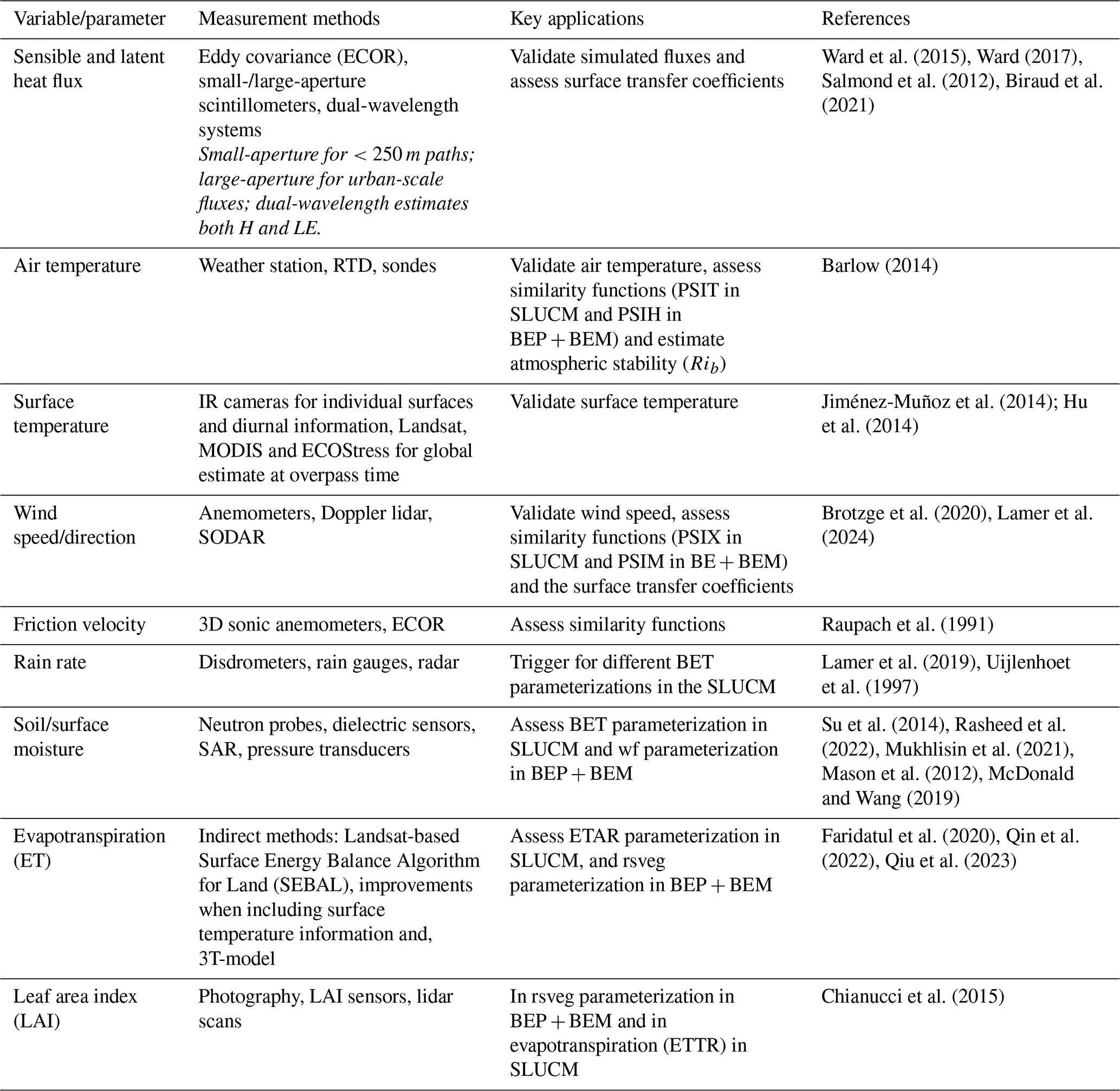
A variety of observational techniques can be employed to evaluate the turbulent flux parameterizations in WRF-Urban. Table 1 summarizes what we believe are key variables, their links to model parameters, recommended instruments, and relevant literature on the techniques.

Ward et al. (2015)Ward (2017)Salmond et al. (2012)Biraud et al. (2021)Barlow (2014)Jiménez-Muñoz et al. (2014); Hu et al. (2014)Brotzge et al. (2020)Lamer et al. (2024)Raupach et al. (1991)Lamer et al. (2019)Uijlenhoet et al. (1997)Su et al. (2014)Rasheed et al. (2022)Mukhlisin et al. (2021)Mason et al. (2012)McDonald and Wang (2019)Faridatul et al. (2020)Qin et al. (2022)Qiu et al. (2023)Chianucci et al. (2015)

Table 1 Observations for informing turbulent flux parameterizations in WRF-Urban.

It is worth nothing that multi-parametric observational datasets are especially useful for diagnosing compensating errors across coupled model components and for evaluating model parameters that are challenging to measure. For example we note that by combining heat flux, air temperature and land surface temperature measurements, the heat transfer coefficients can be evaluated. For example, Bruno et al. (2022) evaluated heat transfer coefficients on building components using measurements collected at an outdoor experimental facility featuring seven monitored building surfaces (walls, floor, ceiling, window, and door). The experiment involved deploying 62 temperature sensors and 13 heat flux meters on internal and external surfaces to monitor thermal exchanges. A weather station was deployed to record outdoor temperature, wind velocity, solar radiation, and sky infrared radiation. Their study showed that windows and doors are more sensitive to radiation and conduction losses than opaque walls, thus suggesting that a single heat transfer coefficient may not be suitable to represent the entire wall surface. They also noted that south-facing walls showed greater heat transfer coefficient fluctuations due to solar radiation suggesting that adding consideration to solar angle may help improve the accuracy of wall heat flux calculations. Such experiments could be repeated for various building types to help inform parameterizations of the heat transfer coefficients, especially the empirical formulation for the heat transfer coefficient of the wall surface (hc) employed in the BEP+BEM which strictly considers wind speed.

As for which urban regimes should be in focus: Given the challenges in estimating integrated similarity functions under very stable or very unstable atmospheric conditions, we believe targeted observations in those regimes would be especially valuable. Also, since the WRF UCMs apply thresholds based on the bulk Richardson number (Ri_b) to switch among similarity functions, observations collected near regime transitions could help determine whether such thresholding is physically justified. Flux-gradient relationships, which form the basis of similarity functions, in urban areas are challenging to evaluate not only due to complex surface conditions and limited observations, but also because urban heterogeneity can lead to space-dependent flux-gradient behavior. Differences in building geometry, surface materials, and vegetation across small spatial scales can alter local turbulence and vertical gradients, complicating the assumption of horizontally homogeneous conditions underlying traditional similarity theory. As a result, evaluating existing flux-gradient formulations requires carefully designed field campaigns that account for spatial variability – such as deploying dense sensor networks or mobile platforms to capture local gradients. These considerations are critical for assessing the validity of parameterizations and improving model performance in heterogeneous urban environments. Finally, we would argue that urban environments with high surface heterogeneity at subgrid scales warrant further study, as they challenge the assumptions of uniform land cover or building morphology inherent to WRF-Urban. Observation-based approaches can assist with estimating similarity relations for momentum by fitting the relationship between the dimensionless wind velocity gradient and local stability parameters using observations spanning from the surface to the top of the roughness sublayer, which is estimated to extend 2−5 times the average building height (Zou et al., 2015; Rotach, 1993; Moriwaki and Kanda, 2006). The dimensionless wind velocity gradient can be determined by (i) fitting wind speed measurements taken at multiple heights to get the wind velocity gradient, (ii) estimating the effective height above the zero-plane displacement height from field surveys, and (iii) calculating the friction velocity . The local stability parameter can be computed following local similarity theory, incorporating key variables such as the effective height above the zero-plane displacement height and the local Obukhov length. The latter derived from measurements of mean virtual potential temperature, kinematic heat flux, and friction velocity obtainable from ultrasonic anemometers. The similarity relation for heat can be similarly estimated with temperature measurement obtained from sonic anemometer or wire thermocouples.

4 Radiative fluxes

4.1 Shortwave radiation parameterizations

4.1.1 BOX 3 – the schematics shown in Fig. 1 illustrate the shortwave radiation exchange between walls and the ground surface, as described by Eqs. (35)–(39)

Likewise, Fig. 2 depicts the radiation interactions between the ground and walls as formulated by the BEP scheme in Eqs. (40)–(42).

Parallels can be drawn between the SLUCM and BEP treatments of shortwave radiation (SWR) balance at surfaces. Both models employ the view factor formulation to represent the proportion of a surface visible from a particular point. Both models also consider SW reflections on the wall and ground surfaces, the SLUCM considers a single reflection, while the BEP model considers reflections at multiple levels. Both models have a simplified treatment of the roof surface, where shadows and reflections from walls are omitted.

In the SLUCM, equations for the SWR absorbed by each surface have a term for the direct (SD) and diffuse (SQ) components of SWR. The total solar SW radiation, provided by the WRF radiative transfer model, is divided into its direct and diffuse components using the SRATIO parameter. By default, SRATIO is set to 75 %, assuming that 75 % of the solar SW radiation is direct and 25 % is diffuse. This formulation oversimplifies several factors influencing the direct-to-diffuse radiation ratio, such as cloud cover, aerosols, and atmospheric conditions, which exhibit significant diurnal and spatio-temporal variability. Observations could help provide guidance as to the true variability of SRATIO and could be used to formulate a parameterization for this parameter (see Sect. 4.3 for additional discussion).

In the SLUCM, the SWR absorbed by the rooftop surface (SR1) and green rooftop surface (SGR1) takes the form:

$$\begin{array}{}\text{(35)}& \begin{array}{rl}\underset{\begin{array}{c}\mathrm{Line}\left[\mathrm{921.922}\right]\\ \mathtt{\text{module\_sf\_urban.F}}\end{array}}{\underbrace{[\mathrm{SR}\mathrm{1},\mathrm{SGR}\mathrm{1}]}}& =\underset{\begin{array}{c}\mathrm{T}\mathrm{1}:\mathrm{Direct}\mathrm{SWR}\mathrm{from}\mathrm{the}\mathrm{sky}\\ \mathrm{absorbed}\mathrm{by}\mathrm{the}\mathrm{roof}\end{array}}{\underbrace{\mathrm{SD}(\mathrm{1}-[\mathrm{ALBR},\mathrm{ALBV}\left]\right)}}\\ & +\underset{\begin{array}{c}\mathrm{T}\mathrm{2}:\mathrm{Diffuse}\mathrm{SWR}\mathrm{from}\mathrm{the}\mathrm{sky}\\ \mathrm{absorbed}\mathrm{by}\mathrm{the}\mathrm{roof}\end{array}}{\underbrace{\mathrm{SQ}(\mathrm{1}-[\mathrm{ALBR},\mathrm{ALBV}\left]\right)}},\end{array}\end{array}$$

where ALBR being the roof albedo, user-defined and specified in the urb_param_table, and ALBV the albedo of the green roof which is set to 0.2 in the module_sf_urban.F.

For surfaces within the urban canyon (ground and wall), the SLUCM model can account for shading effects – if this option is turned on using the shadow_flag parameter – and for a single reflection. This gives rise to more terms in equations describing the SWR absorbed by these surfaces. For the ground:

$$\begin{array}{}\text{(36)}& {\displaystyle }\begin{array}{rl}& \underset{\begin{array}{c}\mathrm{Line}\mathrm{923}\\ \mathtt{\text{module\_sf\_urban.F}}\end{array}}{\underbrace{\mathrm{SG}\mathrm{1}}}\\ & =\underset{\begin{array}{c}\mathrm{T}\mathrm{1}:\mathrm{Direct}\mathrm{SWR}\mathrm{from}\mathrm{the}\mathrm{sky}\mathrm{on}\mathrm{the}\mathrm{lit}\mathrm{portion}\mathrm{of}\\ \mathrm{the}\mathrm{ground}\mathrm{absorbed}\mathrm{by}\mathrm{the}\mathrm{ground}\end{array}}{\underbrace{\mathrm{SD}{\displaystyle \frac{\mathrm{RW}-\mathrm{SLX}}{\mathrm{RW}}}(\mathrm{1}-\mathrm{ALBG})}}\\ & +\underset{\begin{array}{c}\mathrm{T}\mathrm{2}:\mathrm{Diffuse}\mathrm{SWR}\mathrm{from}\mathrm{the}\mathrm{sky}\mathrm{seen}\mathrm{\&}\\ \mathrm{absorbed}\mathrm{by}\mathrm{the}\mathrm{ground}\end{array}}{\underbrace{\mathrm{SQ}\times \mathrm{VFGS}(\mathrm{1}-\mathrm{ALBG})}},\end{array}\text{(37)}& {\displaystyle }\begin{array}{rl}& \underset{\begin{array}{c}\mathrm{Line}\mathrm{925}\\ \mathtt{\text{module\_sf\_urban.F}}\end{array}}{\underbrace{\mathrm{SG}\mathrm{2}}}\\ & =\underset{\begin{array}{c}\mathrm{T}\mathrm{1}:\mathrm{Direct}\mathrm{SWR}\mathrm{from}\mathrm{the}\mathrm{sky}\mathrm{incident}\mathrm{on}\mathrm{the}\mathrm{lit}\mathrm{portion}\mathrm{of}\mathrm{the}\\ \mathrm{wall}\mathrm{reflected}\mathrm{towards}\mathrm{the}\mathrm{ground}\mathrm{and}\mathrm{absorbed}\mathrm{by}\mathrm{the}\mathrm{ground}\end{array}}{\underbrace{\mathrm{SD}{\displaystyle \frac{\mathrm{SLX}}{W}}\times \mathrm{ALBB}\times \mathrm{VFGW}(\mathrm{1}-\mathrm{ALBG})}}\\ & +\underset{\begin{array}{c}\mathrm{T}\mathrm{2}:\mathrm{Diffuse}\mathrm{SWR}\mathrm{from}\mathrm{the}\mathrm{sky}\mathrm{seen}\mathrm{by}\mathrm{the}\mathrm{wall}\mathrm{reflected}\\ \mathrm{towards}\mathrm{the}\mathrm{ground}\mathrm{and}\mathrm{absorbed}\mathrm{by}\mathrm{the}\mathrm{ground}\end{array}}{\underbrace{\mathrm{SQ}\times \mathrm{VFWS}\times \mathrm{ALBB}\times \mathrm{VFGW}(\mathrm{1}-\mathrm{ALBG})}},\end{array}\end{array}$$

with ALBG being the ground albedo and ALBB the wall albedo both user-defined and specified in the urb_param_table. The first terms in Eqs. (36) and (37) depend on the ratio of the shadow length (SLX) to the normalized surface length or in other words the illuminated fraction of the surface. The normalized canyon width (RW) is employed in the estimation of SWR at the ground surface, while the normalized building height  W) is employed in the estimate of the SWR at the wall surface with the factor of two representing contributions from both walls (2 ⋅ normalized height). The shadow length (SLX) is influenced by several factors, including latitude, solar zenith angle, solar hour angle, building height, street width, and street orientation, and is estimated between line 884 and 919 within the module_sf_urban.F. Most terms consider a view factor depending on the surface viewing the radiation. VFGS represents how the ground views the sun, VFGW represents how the ground views the wall and VFWS represents how the wall views the sun.

For the wall surface, the SLUCM further considers one reflection between the East and West wall, which gives rise to two additional terms in the equation for SWR absorbed by the wall surface (SB), one for the direct and one for the diffuse component of SWR:

$$\begin{array}{}\text{(38)}& \begin{array}{rl}& \underset{\begin{array}{c}\mathrm{Line}\mathrm{924}\\ \mathtt{\text{module\_sf\_urban.F}}\end{array}}{\underbrace{\mathrm{SB}\mathrm{1}}}\\ & =\underset{\begin{array}{c}\mathrm{T}\mathrm{1}:\mathrm{Direct}\mathrm{SWR}\mathrm{from}\mathrm{the}\mathrm{sky}\mathrm{incident}\mathrm{on}\mathrm{the}\mathrm{lit}\\ \mathrm{portion}\mathrm{of}\mathrm{the}\mathrm{wall}\mathrm{absorbed}\mathrm{by}\mathrm{the}\mathrm{wall}\end{array}}{\underbrace{\mathrm{SD}{\displaystyle \frac{\mathrm{SLX}}{W}}(\mathrm{1}-\mathrm{ALBB})}}\\ & +\underset{\begin{array}{c}\mathrm{T}\mathrm{2}:\mathrm{Diffuse}\mathrm{SWR}\mathrm{from}\mathrm{the}\mathrm{sky},\mathrm{seen}\mathrm{\&}\\ \mathrm{absorbed}\mathrm{by}\mathrm{the}\mathrm{wall}\end{array}}{\underbrace{\mathrm{SQ}\times \mathrm{VFWS}(\mathrm{1}-\mathrm{ALBB})}},\end{array}\end{array}$$

$$\begin{array}{}\text{(39)}& \begin{array}{rl}& \underset{\begin{array}{c}\mathrm{Line}\mathrm{926}\\ \mathtt{\text{module\_sf\_urban.F}}\end{array}}{\underbrace{\mathrm{SB}\mathrm{2}}}\\ & =\underset{\begin{array}{c}\mathrm{T}\mathrm{1}:\mathrm{Direct}\mathrm{SWR}\mathrm{from}\mathrm{the}\mathrm{sky}\mathrm{incident}\mathrm{on}\mathrm{the}\mathrm{lit}\mathrm{portion}\mathrm{of}\mathrm{the}\mathrm{ground}\\ \mathrm{reflected}\mathrm{towards}\mathrm{the}\mathrm{wall}\mathrm{\&}\mathrm{absrobed}\mathrm{by}\mathrm{the}\mathrm{wall}\end{array}}{\underbrace{\mathrm{SD}{\displaystyle \frac{\mathrm{RW}-\mathrm{SLX}}{\mathrm{RW}}}\times \mathrm{ALBG}\times \mathrm{VFWG}(\mathrm{1}-\mathrm{ALBB})}}\\ & +\underset{\begin{array}{c}\mathrm{T}\mathrm{2}:\mathrm{Diffuse}\mathrm{SWR}\mathrm{from}\mathrm{the}\mathrm{sky}\mathrm{seen}\mathrm{by}\mathrm{the}\mathrm{ground}\mathrm{reflected}\\ \mathrm{towards}\mathrm{the}\mathrm{wall}\mathrm{\&}\mathrm{absorbed}\mathrm{by}\mathrm{the}\mathrm{wall}\end{array}}{\underbrace{\mathrm{SQ}\times \mathrm{VFGS}\times \mathrm{ALBG}\times \mathrm{VFWG}(\mathrm{1}-\mathrm{ALBB})}}\\ & +\underset{\begin{array}{c}\mathrm{T}\mathrm{3}:\mathrm{Direct}\mathrm{SWR}\mathrm{from}\mathrm{the}\mathrm{sky}\mathrm{incident}\mathrm{on}\mathrm{the}\mathrm{lit}\mathrm{portion}\mathrm{of}\mathrm{the}\mathrm{wall}\mathrm{reflected}\\ \mathrm{towards}\mathrm{the}\mathrm{other}\mathrm{wall}\mathrm{absorbed}\mathrm{by}\mathrm{the}\mathrm{wall}:\mathrm{added}\mathrm{to}\mathrm{WRF}\mathrm{v}\mathrm{4.6.1}\end{array}}{\underbrace{\mathrm{SD}{\displaystyle \frac{\mathrm{SLX}}{W}}\mathrm{ALBB}\times \mathrm{VFWW}(\mathrm{1}-\mathrm{ALBB})}}\\ & +\underset{\begin{array}{c}\mathrm{T}\mathrm{4}:\mathrm{Diffuse}\mathrm{SWR}\mathrm{from}\mathrm{the}\mathrm{sky}\mathrm{seen}\mathrm{by}\mathrm{the}\mathrm{wall}\mathrm{reflected}\mathrm{towards}\mathrm{the}\\ \mathrm{other}\mathrm{wall}\mathrm{absorbed}\mathrm{by}\mathrm{that}\mathrm{wall}:\mathrm{added}\mathrm{to}\mathrm{WRF}\mathrm{v}\mathrm{4.6.1}\end{array}}{\underbrace{\mathrm{SQ}\times \mathrm{VFWS}\times \mathrm{ALBB}\times \mathrm{VFWW}(\mathrm{1}-\mathrm{ALBB})}},\end{array}\end{array}$$

where VFWW represents the view factor from one wall to the other.

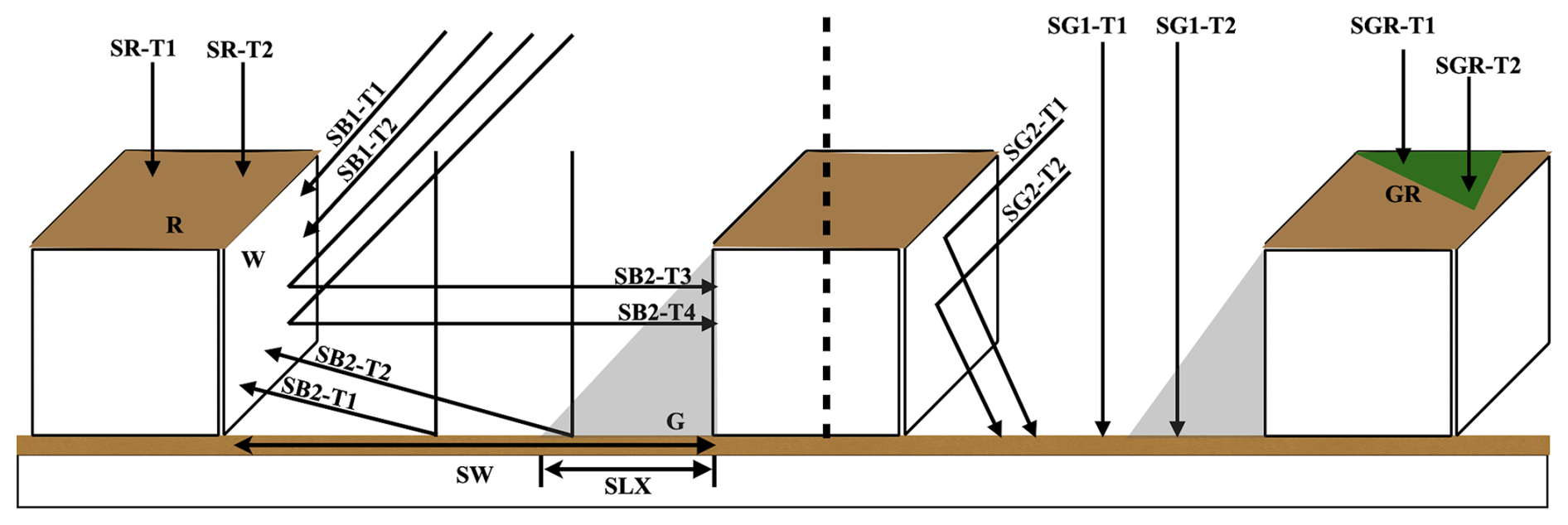
Figure 1 Schematic representation of SWR exchange in the SLUCM model. Depicted are the components of the SWR absorbed by the roof (SR), green roof (SGR), ground (SG), and wall (SB) surfaces in the SLUCM. The components are labeled to refer to the terms in the equations within this subsection; for instance, SG-T1 refers to the first term of the first equation describing the SWR absorbed by the ground surface in the SLUCM (i.e., Eq. 46). The gray triangle in the figure represent the shadow cast on the street and wall surfaces. The green triangle represents the green roof.

Unlike the SLUCM, the BEP model estimates the SWR incident on its surfaces at each urban grid level by solving a system of equations simultaneously, factoring in the probability of buildings being equal to height of a given level (pb(z_ju+1)). This concept is implemented as a system of equations in the form [A]X=[B]. Here, [A] represents a $(\mathrm{2}\cdot \mathrm{nz}\mathrm{\_}\mathrm{u}+\mathrm{1})\times (\mathrm{2}\cdot \mathrm{nz}\mathrm{\_}\mathrm{u}+\mathrm{1})$ coefficient matrix for the SWR flux at the east and west walls and the ground (rsw^W, rsw^E, and rsg), nz_u is the number of urban vertical layers. The [B] array with a of size $(\mathrm{2}\cdot \mathrm{nz}\mathrm{\_}\mathrm{u}+\mathrm{1})\times \mathrm{1}$ includes the downward SWR from the sky incident on the walls and the ground. To facilitate explanation, this system of equations is decomposed into its components. The subscripts s→iu, s→ju, and s→g are used to indicate the direction of radiation transport: from the sky to the iuth-element of the wall, the sky to the juth-element of the opposite wall, the ju^th-element of the opposite wall to the ground, and the sky to the ground, respectively. Here, iu and ju denotes the iuth-element (or level) of the current wall and the juth-element (or level) of the opposite wall, respectively.

Another key distinction between the SLUCM and the BEP model is that BEP computes the incident (not the absorbed) SWR on each surface. The incident SWR is converted into the absorbed SW radiation for each surface by considering their albedo during the estimation of each surface's temperature. BEP accounts for the impact of shadows on the direct SWR in an independent step before estimating the incident SWR balance for each surface. The computation of direct SWR incident on the illuminated portion of the ground (rsg_s→g) and of the West wall (rsw${}_{\mathrm{s}\to \mathrm{iu}}^{\mathrm{W}}$) of the East wall (rsw${}_{\mathrm{s}\to \mathrm{iu}}^{\mathrm{E}}$) considers the canyon orientation:

$$\begin{array}{}\text{(40)}& {\displaystyle }& {\displaystyle }\underset{\begin{array}{c}\mathrm{Line}\mathrm{3301}\\ \mathtt{\text{module\_sf\_bep\_bem.F}}\end{array}}{\underbrace{{\mathrm{rsw}}_{\mathrm{s}\to \mathrm{iu}}^{\mathrm{W}}}}=\mathrm{swddir}\times \mathrm{rd}\times \mathrm{ss}/\mathrm{pb},\text{(41)}& {\displaystyle }& {\displaystyle }\underset{\begin{array}{c}\mathrm{Line}\mathrm{3311}\\ \mathtt{\text{module\_sf\_bep\_bem.F}}\end{array}}{\underbrace{{\mathrm{rsg}}_{\mathrm{s}\to \mathrm{g}}}}=\mathrm{swddir}\cdot \mathrm{rd}\cdot \mathrm{ss}/\mathrm{wsd},\end{array}$$

where swddir is the downward direct shortwave radiation, ss is the probability of the buildings with height equal to a given urban grid level, pb is the probability of the buildings with height equal to and taller than the given urban grid level, wsd represent the street width divided by the sine of the angle between direction of the sun and the face of the wall that accounts for the canyon orientation, rd is the ratio of portion of the wall lit to the horizontal surface illuminated area, that account for the shadow effect. Ultimately all orientations are averaged over the cell, considering the areas occupied by canyons with different orientations.

The SW radiation incident on the ground surface (rsg) is comprised of three components (see Eq. S3) while the SW radiation budget incorporates an additional term to account for SW radiation reflected from the opposite wall onto the wall of interest. Below, the formulation for the SW radiation budget of the West wall (rsw${}_{\mathrm{iu}}^{\mathrm{W}}$) is presented; the East wall follows an identical formulation with the indices [E, W] interchanged:

$$\begin{array}{}\text{(42)}& \begin{array}{rl}& \underset{\begin{array}{c}\mathrm{Line}\mathrm{3652},\mathrm{3656}\\ \mathtt{\text{module\_sf\_bep\_bem.F}}\end{array}}{\underbrace{{\mathrm{rsw}}_{\mathrm{iu}}^{\mathrm{W}}}}\\ & =\underset{\begin{array}{c}\mathrm{T}\mathrm{1}:\mathrm{SWR}\mathrm{incident}\mathrm{on}\mathrm{the}\mathrm{illuminated}\mathrm{portion}\mathrm{of}\mathrm{the}\\ \mathrm{west}\mathrm{wall}\mathrm{at}\mathrm{level}iu\mathrm{considering}\mathrm{the}\mathrm{effect}\mathrm{of}\mathrm{shadows}\end{array}}{\underbrace{{\mathrm{rsw}}_{\mathrm{s}\to \mathrm{iu}}^{\mathrm{W}}}}\\ & +\underset{\begin{array}{c}\mathrm{T}\mathrm{2}:\mathrm{Diffuse}\mathrm{SWR}\mathrm{from}\mathrm{the}\mathrm{sky}\\ \mathrm{to}\mathrm{the}iu\mathrm{level}\mathrm{of}\mathrm{the}\mathrm{west}\mathrm{wall}\end{array}}{\underbrace{{\mathrm{rsdif}}_{\mathrm{s}\to \mathrm{iu}}^{\mathrm{W}}\times \mathrm{fsw}}}\\ & +\underset{\begin{array}{c}\mathrm{T}\mathrm{3}:\mathrm{Total}\mathrm{SWR}\mathrm{at}\mathrm{the}\mathrm{ground}\\ \mathrm{reflected}\mathrm{towards}\mathrm{the}\mathrm{wall}\end{array}}{\underbrace{\mathrm{rsg}\times \mathrm{albg}\times \mathrm{fgw}}}\\ & +\underset{\begin{array}{c}\mathrm{T}\mathrm{4}:\mathrm{Total}\mathrm{SWR}\mathrm{at}\mathrm{the}\mathrm{east}\mathrm{wall}\\ \mathrm{reflected}\mathrm{towards}\mathrm{the}\mathrm{west}\mathrm{wall}\mathrm{by}\mathrm{the}\mathrm{portion}\mathrm{of}\mathrm{buildings}\mathrm{at}\mathrm{that}\mathrm{level}\end{array}}{\underbrace{\sum _{\mathrm{ju}=\mathrm{1},\mathrm{nu}}{\mathrm{rsw}}_{\mathrm{ju}}^{\mathrm{E}}\times \mathrm{pb}\left(z_{\mathrm{ju}+\mathrm{1}}\right)\mathrm{albw}\times \mathrm{fww}}},\end{array}\end{array}$$

with fgw denoting the view factors of the wall looking at the ground, fww the view factor between the wall and the opposite wall, fsw is the view factor of the wall looking at the sky, fsg is the view factor of the ground looking at the sky, and albg is the albedo of the ground surface. Notably, the BEP (or BEP − BEM) formulation uses fewer terms than the SLUCM approach because it employs the total SW radiation at the building wall to estimate the SW radiation reaching the ground, rather than recalculating each component of wall SW radiation (both direct and diffuse).

.

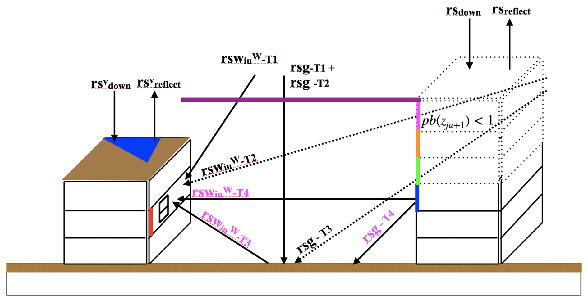
Figure 2 Schematic representation of SWR exchange in the BEP model. Depicted are the components of the incident SWR on the roof (rs), photovoltaic panel (rsv), ground (rsg) and wall (rsw) surfaces. The components are labeled to refer to the terms in the equations within this subsection; for instance, rsg-T1 refers to the first term of the first equation describing the SWR incident on the ground surface in the BEP (i.e., Eq. 43). Dashed building floors represent the probabilistic approach used to account for radiation not blocked by buildings (i.e., (pb(z)<1). Purple labels refer to the components that use the total surface SWR rather than the sky SWR

4.2 Longwave radiation parameterizations

4.2.1 BOX 4 – similarly to the shortwave radiation section, the schematics in Fig. 3 correspond to Eqs. (43)–(45), illustrating the longwave radiation exchange between the walls and the ground surface, whereas Fig. 4 depicts the longwave radiation interactions between the ground and walls represented by the BEP scheme, as formulated in Eq. (46)

Similar to the formulation for the SWR balance on each surface, the formulation for the longwave radiation (LWR) balance on each surface in the SLUCM and BEP employs the view factor formulation to represent the proportion of a surface visible from a particular point. Both models also consider LWR reflections on the wall and ground surfaces, the SLUCM considers a single reflection, while the BEP model considers several reflections at multiple levels. Both models have a simplified treatment of the roof surface, where reflections from walls are omitted.

In the SLUCM, this approach leads to the following formulation of the net LWR for the roof surface (RR):

$$\begin{array}{}\text{(43)}& \underset{\begin{array}{c}\mathrm{Line}\mathrm{1026}\\ \mathtt{\text{module\_sf\_urban.F}}\end{array}}{\underbrace{\mathrm{RR}}}=\mathrm{EPSR}\left(\underset{\begin{array}{c}\mathrm{T}\mathrm{1}:\mathrm{LWR}\mathrm{from}\\ \mathrm{sky}\mathrm{to}\mathrm{roof}\end{array}}{\underbrace{\mathrm{RX}}}-\underset{\begin{array}{c}\mathrm{T}\mathrm{2}:\mathrm{LWR}\mathrm{from}\\ \mathrm{roof}\mathrm{to}\mathrm{sky}\end{array}}{\underbrace{\mathrm{SIG}\times {\mathrm{TRP}}^{\mathrm{4}}}}\right),\end{array}$$

where RX represents the total downward LWR from the sky, which is supplied to the SLUCM model by the WRF atmospheric radiation scheme. The emissivity of the roof surface EPSR and of the ground surface EPSG and of the wall EPSB is specified by the user in the urb_param_table. The outgoing LWR flux (RR-T2) is influenced by the roof surface temperature (TRP) from the previous time step and involves the Stefan–Boltzmann constant (SIG).

The net LWR at the ground surface (RG) has additional terms to account for LWR emitted from the wall surface towards the ground surface (RG1-T2) as well as for reflected LWR reaching the ground surface (RG2) (see Eqs. S4 and S5) while the net LWR at the wall (RB) has additional terms to account for LWR emitted by and reflected from the opposite wall. All LWR reaching the wall from reflection are contained in RB2:

$$\begin{array}{}\text{(44)}& {\displaystyle }\begin{array}{rl}& \underset{\begin{array}{c}\mathrm{Line}\mathrm{1288}\\ \mathtt{\text{module\_sf\_urban.F}}\end{array}}{\underbrace{\mathrm{RB}\mathrm{1}}}=\mathrm{EPSB}(\underset{\begin{array}{c}\mathrm{T}\mathrm{1}:\mathrm{LWR}\mathrm{from}\mathrm{sky}\\ \mathrm{seen}\mathrm{by}\mathrm{wall}\end{array}}{\underbrace{\mathrm{RX}\times \mathrm{VFWS}}}\\ & +\underset{\begin{array}{c}\mathrm{T}\mathrm{2}:\mathrm{LWR}\mathrm{from}\mathrm{ground}\\ \mathrm{seen}\mathrm{by}\mathrm{wall}\end{array}}{\underbrace{\mathrm{EPSG}\times \mathrm{SIG}\times {\mathrm{TGP}}^{\mathrm{4}}\times \mathrm{VFWG}}}\\ & +\underset{\begin{array}{c}\mathrm{T}\mathrm{3}:\mathrm{LWR}\mathrm{from}\mathrm{opposite}\\ \mathrm{wall}\mathrm{seen}\mathrm{by}\mathrm{wall}\end{array}}{\underbrace{\mathrm{EPSB}\times \mathrm{SIG}\times {\mathrm{TBP}}^{\mathrm{4}}\times \mathrm{VFWW}}}-\underset{\begin{array}{c}\mathrm{T}\mathrm{4}:\mathrm{LWR}\mathrm{from}\\ \mathrm{wall}\mathrm{out}\end{array}}{\underbrace{\mathrm{SIG}\times {\mathrm{TBP}}^{\mathrm{4}}}}).\end{array}\text{(45)}& {\displaystyle }\begin{array}{rl}& \underset{\begin{array}{c}\mathrm{Line}\mathrm{1297}\\ \mathtt{\text{module\_sf\_urban.F}}\end{array}}{\underbrace{\mathrm{RB}\mathrm{2}}}\\ & =\mathrm{EPSB}(\underset{\begin{array}{c}\mathrm{T}\mathrm{1}:\mathrm{LWR}\mathrm{from}\mathrm{sky}\mathrm{seen}\mathrm{by}\\ \mathrm{ground}\mathrm{reflected}\mathrm{towards}\mathrm{wall}\end{array}}{\underbrace{\mathrm{RX}\times \mathrm{VFGS}(\mathrm{1}-\mathrm{EPSG})\mathrm{VFWG}}}\\ & +\underset{\begin{array}{c}\mathrm{T}\mathrm{2}:\mathrm{LWR}\mathrm{from}\mathrm{wall}\mathrm{seen}\mathrm{by}\mathrm{ground}\\ \mathrm{reflected}\mathrm{towards}\mathrm{wall}\end{array}}{\underbrace{\mathrm{EPSB}\times \mathrm{SIG}\times {\mathrm{TBP}}^{\mathrm{4}}\times \mathrm{VFGW}(\mathrm{1}-\mathrm{EPSG})\mathrm{VFWG}}}\\ & +\underset{\begin{array}{c}\mathrm{T}\mathrm{3}:\mathrm{LWR}\mathrm{from}\mathrm{sky}\mathrm{seen}\mathrm{by}\mathrm{opposite}\\ \mathrm{wall}\mathrm{reflected}\mathrm{towards}\mathrm{wall}\end{array}}{\underbrace{\mathrm{RX}\times \mathrm{VFWS}(\mathrm{1}-\mathrm{EPSB})\mathrm{VFWW}}}\\ & +\underset{\begin{array}{c}\mathrm{T}\mathrm{4}:\mathrm{LWR}\mathrm{from}\mathrm{ground}\mathrm{seen}\mathrm{by}\mathrm{opposite}\\ \mathrm{wall}\mathrm{reflected}\mathrm{towards}\mathrm{wall}\end{array}}{\underbrace{\mathrm{EPSG}\times \mathrm{SIG}\times {\mathrm{TGP}}^{\mathrm{4}}\times \mathrm{VFWG}(\mathrm{1}-\mathrm{EPSB})\mathrm{VFWW}}}\\ & +\underset{\begin{array}{c}\mathrm{T}\mathrm{5}:\mathrm{LWR}\mathrm{from}\mathrm{opposite}\mathrm{wall}\mathrm{seen}\mathrm{by}\mathrm{wall}\\ \mathrm{reflected}\mathrm{towards}\mathrm{opposite}\mathrm{wall}\end{array}}{\underbrace{\mathrm{EPSB}\times \mathrm{SIG}\times {\mathrm{TBP}}^{\mathrm{4}}\times \mathrm{VFWW}(\mathrm{1}-\mathrm{EPSB})\mathrm{VFWW}}}).\end{array}\end{array}$$

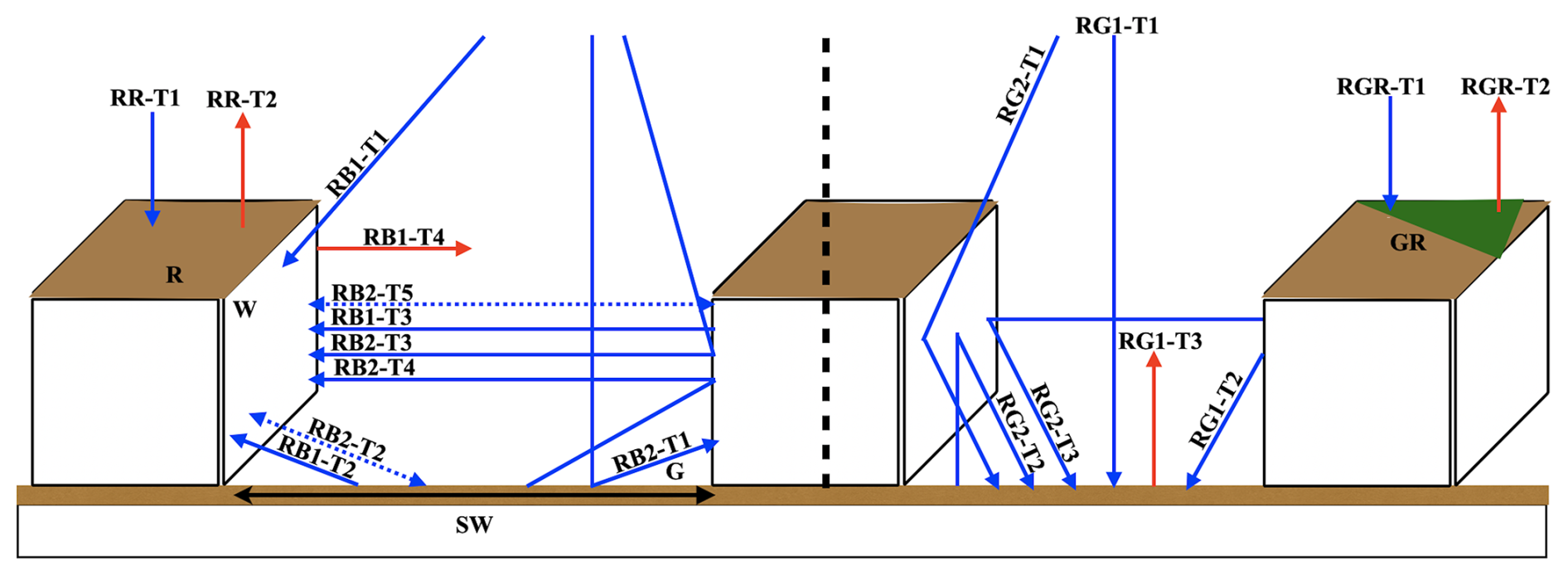
Figure 3 Schematic representation of LWR exchange in the SLUCM model. Depicted are the components of the LWR balance at the roof (RR), green roof (RGR), ground (RG) and wall (RB) surfaces. The components are labeled to refer to the terms in the equations within this subsection; for instance, RG1-T1 refers to the first term of the first equation describing the net LWR at the ground surface in the SLUCM (i.e., Eq. 42). Blue arrows represent incoming LWR, while red arrows indicate outgoing LWR. Dashed double-sided arrows depict radiation leaving a surface and being reflected back to it. The green triange represents a green roof.

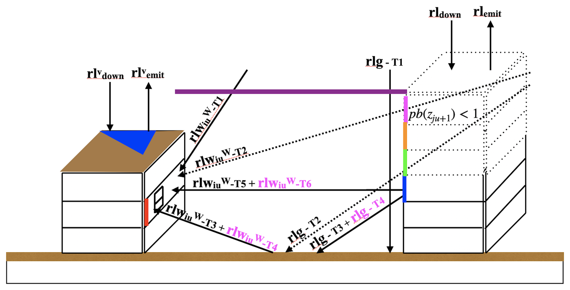
Figure 4 Schematic representation of LWR exchange in the BEP model. Depicted are the components of the incident SWR on the roof (rl), photovoltaic (PV) panel (rlv), ground (rlg) and wall (rlw) surfaces. The components are labeled to refer to the terms in the equations within this subsection; for instance, rlg-T1 refers to the first term of the first equation describing the LWR incident on the ground surface in the BEP (i.e., Eq. 46). Dashed building floors represent the probabilistic approach used to account for radiation not blocked by buildings (i.e., pb(z)<1). The blue triangle represent a PV panel.

As it does to estimate the SWR incident on its various surface, the BEP (or BEP-BEM) model estimates the incident LWR at its various surfaces at its different levels using a system of equations, factoring in the probability of buildings being equal to height of a given level. Another key distinction between the SLUCM and the BEP model is that BEP computes the incident (not the net) LWR on each surface. The incident LWR is converted into the net LW radiation for each surface by considering their emissivity during the estimation of each surface's temperature.

The BEP-BEM module further considers the presence of windows on building walls. Windows are treated as another surface, with their own temperature twlev, and emissivity emwin and are set to cover a fraction of the wall pwin. The emissivity of the wall is denoted by emw while the wall temperature is given by tw. The parameter sigma ($=\mathrm{5.67}\times {\mathrm{10}}^{-\mathrm{8}}$) is the Stefan–Boltzmann constant.

As a result, the incident LWR at the ground surface (rlg) is comprised of four components, including a weighted average of the contribution of the wall and window surface (see Eq. S6) and the incident LWR at the west wall surface (rlw^W) is comprised of two more components to account for the effect of the East wall:

$$\begin{array}{}\text{(46)}& \begin{array}{rl}& \underset{\begin{array}{c}\mathrm{Lines}:\mathrm{3535},\mathrm{3539}\\ \mathtt{\text{module\_sf\_bep\_bem.F}}\end{array}}{\underbrace{{\mathrm{rlw}}_{\mathrm{iu}}^{\mathrm{W}}}}=\underset{\begin{array}{c}\mathrm{T}\mathrm{1}:\mathrm{LWR}\mathrm{from}\mathrm{sky}\\ \mathrm{seen}\mathrm{by}\mathrm{west}\mathrm{wall}\end{array}}{\underbrace{\mathrm{rl}\times \mathrm{fsw}}}\\ & +\underset{\begin{array}{c}\mathrm{T}\mathrm{2}:\mathrm{Portion}\mathrm{of}\mathrm{sky}\mathrm{LWR}\mathrm{that}\mathrm{passed}\\ \mathrm{through}\mathrm{east}\mathrm{walls}\mathrm{that}\mathrm{is}\mathrm{seen}\mathrm{by}\mathrm{west}\mathrm{wall}\end{array}}{\underbrace{\sum _{\mathrm{ju}=\mathrm{1},\mathrm{nu}}\mathrm{rl}\left(\mathrm{1}-\mathrm{pb}\left(z_{\mathrm{ju}+\mathrm{1}}\right)\right)\mathrm{fww}}}\\ & +\underset{\begin{array}{c}\mathrm{T}\mathrm{3}:\mathrm{LWR}\mathrm{emitted}\mathrm{by}\mathrm{ground}\\ \mathrm{seen}\mathrm{by}\mathrm{west}\mathrm{wall}\end{array}}{\underbrace{\mathrm{emg}\times \mathrm{sigma}\times \mathrm{tg}\mathrm{\_}{\mathrm{av}}^{\mathrm{4}}\times \mathrm{fgw}}}+\underset{\begin{array}{c}\mathrm{T}\mathrm{4}:\mathrm{Total}\mathrm{LWR}\mathrm{at}\mathrm{the}\mathrm{ground}\\ \mathrm{reflected}\mathrm{to}\mathrm{west}\mathrm{wall}\end{array}}{\underbrace{\mathrm{rlg}(\mathrm{1}-\mathrm{emg})\mathrm{fgw}}}\\ & +\underset{\begin{array}{c}\mathrm{T}\mathrm{5}:\mathrm{LWR}\mathrm{emitted}\mathrm{by}\mathrm{east}\mathrm{wall}\\ \mathrm{that}\mathrm{is}\mathrm{seen}\mathrm{by}\mathrm{west}\mathrm{wall}\end{array}}{\underbrace{\sum _{\mathrm{ju}=\mathrm{1},\mathrm{nu}}\mathrm{sigma}\times \left(\mathrm{emw}(\mathrm{1}-\mathrm{pwin}){\mathrm{tw}}^{{}^{\mathrm{4}},\mathrm{E}}+\mathrm{emwin}\times \mathrm{pwin}\times {\mathrm{twlev}}^{{}^{\mathrm{4}},\mathrm{E}}\right)\mathrm{pb}\left(z_{\mathrm{ju}+\mathrm{1}}\right)\mathrm{fww}}}\\ & +\underset{\begin{array}{c}\mathrm{T}\mathrm{6}:\mathrm{Total}\mathrm{LWR}\mathrm{at}\mathrm{the}\mathrm{east}\mathrm{wall}\\ \mathrm{reflected}\mathrm{to}\mathrm{west}\mathrm{wall}\end{array}}{\underbrace{\sum _{\mathrm{ju}=\mathrm{1},\mathrm{nu}}{\mathrm{rlw}}^{\mathrm{E}}\times \mathrm{pb}\left(z_{\mathrm{ju}+\mathrm{1}}\right)(\mathrm{1}-\mathrm{emw}(\mathrm{1}-\mathrm{pwin})-\mathrm{emwin}\cdot \mathrm{pwin})\mathrm{fww}}},\end{array}\end{array}$$

where tg is the temperature of the ground surface in the previous time step. A similar equation exists for the east wall, where the “W” and “E” superscripts are interchanged. The discussions on radiative exchange between surfaces in SLUCM and BEP clearly demonstrate that the added complexity of BEP and MLUCM in modeling radiative transfer may offer greater benefits in urban environments with mixed building heights and complex geometries. However, the trade-off between model realism and computational cost should be carefully considered when setting up simulations for a specific city. A systematic evaluation of model performance versus complexity can help guide the choice of urban scheme.

4.3 Observational approaches

Observations can play a crucial role in evaluating the net SWR and LWR simulated for various surface types in WRF-Urban. Furthermore, they can be used to assess their parameterizations via measurements of shadow length and view factor. Observations could also be used to evaluate the impact of omitting reflections and shading on roof surfaces and the use of a fixed ratio (SRATIO) to separate solar radiation into its direct and diffuse components in the SLUCM.

Strategically positioned radiometers would allow us to measure incident and reflected SWR on various urban surfaces (Aoki and Mizutani, 2015). For wall surfaces, mounting a pyranometers facing outward from the wall, aligned with the wall's vertical plane, would provide a measurement of direct sunlight plus diffuse sky radiation (Oliveira et al., 2024). Another pyranometer, positioned at the same height but facing toward the wall, would measure radiation reflected from the wall. A shading structure can be employed to ensure that the pyranometer facing the wall captures only reflected radiation by blocking direct sunlight. To improve accuracy, the pyranometer should be positioned a short distance (10–20 cm) away from the wall to avoid obstruction effects. Similarly, using a pyrgeometer in this setup allows for the measurement of incident and outgoing LWR on the wall surface.

Radiometers are once again useful to measure the ratio of direct to diffuse solar radiation (Kassianov et al., 2024). One common approach involves using a pyranometer equipped with a shadow-band to obstruct direct sunlight, thereby isolating diffuse irradiance measurements. However, this method requires correction factors to account for the portion of the sky occluded by the shadow-band. Another technique employs a pyrheliometer in conjunction with a pyranometer (Wang et al., 2013). The pyrheliometer, aligned with the sun, measures direct normal irradiance, while the pyranometer captures global horizontal irradiance. By subtracting the direct component (adjusted for the solar zenith angle) from the global measurement, it is possible to derive diffuse horizontal irradiance. Additionally, rotating shadowband radiometers (RSRs) have been developed to automate the simultaneous measurement of global, direct, and diffuse irradiance components (Alexandrov et al., 2002). These instruments utilize a rotating shadowband to intermittently shade the sensor, facilitating the differentiation between direct and diffuse radiation. The efficacy of RSRs in measuring diffuse solar irradiance has been evaluated in various studies, highlighting their utility in solar radiation research. Each of these methodologies offers distinct advantages and considerations, with the choice of technique often influenced by the specific requirements of the study and the available instrumentation.

Estimating shadow length in urban street canyons can be achieved through photographic methods with reference scaling. This approach involves capturing images of the area and using known dimensions within the image to scale and measure shadow lengths accurately.

Regarding the estimation of SVF, several methods have been developed and compared in the literature. Geometric methods involve calculating SVF based on the dimensions and arrangement of urban structures. Fish-eye photographic methods use hemispherical images to determine the proportion of visible sky. Global Positioning System (GPS) methods estimate SVF by analyzing positional data. Simulation methods utilize 3D city models or digital surface models to compute SVF. Big data approaches leverage street view images and deep learning algorithms to estimate SVF across large urban areas. A comprehensive review of these methods, including their principles, input data requirements, application contexts, accuracy, and efficiency, is provided by Miao et al. (2020).

5 Summary and conclusions

Despite their broad application and widespread user base, the urban schemes within the WRF physics suite remain comparatively less documented, especially when it comes to the specific implementation of the parameterizations. This article serves two primary purposes.

First, it improves the transparency of the Bulk, Single Layer Urban Canopy Model (SLUCM) and Building Effect Parameterization coupled with Building Energy Model (BEM) model treatment of turbulent and radiative fluxes by creating a faithful roadmap to the code version v4.5.2 with matching symbols and code line number references. We bring the specific code implementation details back to the physics by providing descriptions and schematics to improve code accessibility to non-expert users. This systematic review of the code uncovered several implementation errors, which have since been addressed and corrected in subsequent versions of WRF (v4.6.0 and v4.6.1; see the appendix).

Second, this work narrowed down to the subset of parameters that can be evaluated using the state-of-the-art observation technique to improve the model performance. We identify several threshold-based parameterizations that can introduce discontinuities in simulations: (i) a rain rate threshold in SLUCM that controls minimum moisture availability and in turn affect latent heat flux, necessitating validation under rainfall conditions above and below 1 mm h⁻¹ (Miao and Chen, 2014); (ii) an assumption that all surfaces are dry in BEP, thus leading to zero latent heat flux, which could lead to model errors especially during and after precipitation events, (iii) SWR partitioning in SLUCM using a fixed direct-to-diffuse ratio, which in turn affects surface air temperature, requiring validation under both clear and cloudy skies; and (iv) the use of bulk Richardson number in all three UCMs to select similarity functions, which impact fluxes and the vertical structure of temperature and wind, warranting model evaluation at transitions between atmospheric stability regimes. The wide use of Monin–Obukov similarity theory for flux calculations in the WRF urban models may also be a source of uncertainty particularly in highly stable and highly unstable atmospheric stability regimes and in environments with strong surface heterogeneity on the scale of the model resolution (i.e., highly variable land use land cover or building height and material at sub-km scale), warranting model evaluation in cities presenting dense building layouts with mixtures of high-rise and low-rise within the same neighborhood (e.g., New York City). We also identify a highly simplified treatment of the radiative balance at roof surfaces in all urban schemes, where the effects of shading and reflections from nearby walls are neglected. The implications of these simplifications can be assessed through targeted observations to evaluate their impact on simulation accuracy.

We offer guidance on how observational data can be used to evaluate and refine model assumptions, such as measurements of surface moisture availability, the direct-to-diffuse radiation ratio, and vertical profiles of air temperature and wind. We encourag the use of multi-parameter observations to identify compensating errors. We recommend collecting data at multiple heights, particularly at the model's lowest atmospheric level, to avoid confounding effects from diagnostic extrapolation schemes. For example, past campaigns employed a combination of tower-based and remote sensing measurements (e.g., the Basel UrBan Boundary Layer Experiment (BUBBLE); Rotach et al., 2005). Given challenges with positioning instrumentation in cities, we are seeing the emergence of mobile platforms, including drones and truck-based remote sensing instrumentation in several modern field campaigns, as demonstrated in field campaigns such as the DOE Southwest Urban Field Laboratory (Southwest Integrated Field Laboratory, 2024) and Urbisphere (Fenner et al., 2024).

Although this study has gone into details about model parameterization/schemes and touched on the topic of observational spatio-temporal coverage and comprehensiveness, other factors also impact model performance. These include boundary conditions (e.g., inflow winds), geographic input data (e.g., topography, land use), model setup choices (e.g., grid resolution), and uncertainties in measurement retrieval methods. These aspects warrant further investigation in future work.

Appendix A

A1 Code fixes and model sensitivity outcomes

This study uncovered several inconsistencies between the urban parameterizations described in the literature and their implementation in WRF-Urban version 4.5.2. These inconsistencies – or also kown as code bugs – are now documented in the WRF community forum as pull 2049, 2038, 2032, and 2101 (https://github.com/wrf-model/WRF/pull/, last access: 2 March 2025) and were corrected in subsequent releases (beginning with v4.6.1). To assess the impact of these bug fixes on simulation outcomes, we conducted a one-week WRF sensitivity experiment centered over Atlanta, GA initialized from 2 August 2015, 0Z with the first 24 h spin-up, capturing both clear-sky and precipitation conditions. Figure A1 illustrates the simulation setup, where Fig. A1a shows the outer and inner domains with their respective resolutions (5 and 1 km), and Fig. A1b displays the spatial distribution of urban fraction.

Bug fixes were grouped in two sets, (i) in Building Energy Model (BEM) where we corrected the coefficients used in calculating the heat transfer coefficient for thermal exchange between the roof surface, PV panels, and the atmosphere using the empirical relation, (ii) in SLUCM where we corrected the stability parameter, Lech's surface functions for momentum and heat, added missing terms in short-wave radiation balance

To demonstrate the impact of these bug fixes we run two sets of simulation, one without the bug fix and one with the bug fix, keeping all other physics and settings the same including the use of: Thompson microphysics scheme (Thompson and Eidhammer, 2014), Mellor-Yamada-Janjic (MYJ) planetary boundary layer scheme (Janjić, 1994), Rapid Radiative Transfer Model (RRTMG) shortwave and longwave radiation scheme (Iacono et al., 2008), and the Noah-MP land surface model (Yang et al., 2011; Niu et al., 2011; He et al., 2023). For the BEP-BEM simulations, we employ a photovoltanic panels cover of 50 %, while in the SLUCM simulations we employ a green roof cover of 50 %.

The results demonstrate that even minor implementation issues can meaningfully influence model output. Fixes to the BEM led to changes in both 2 m air temperature (Fig. A2b) and skin temperature on the order of 0.3 K (Fig. A2d) both in urban grids and non-urban grids. Fixes to the SLUCM produced smaller but still notable effects, with temperature changes up to 0.15 K (Fig. A3b and d).

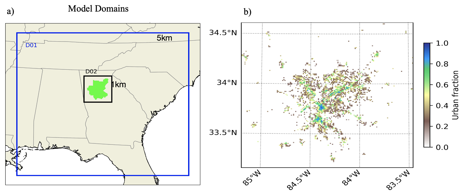
Figure A1 Panel (a) shows the outer (D01) and inner (D02) domains, with horizontal grid resolutions annotated for the WRF test simulations. Panel (b) displays the urban fraction contours within the D02 domain.

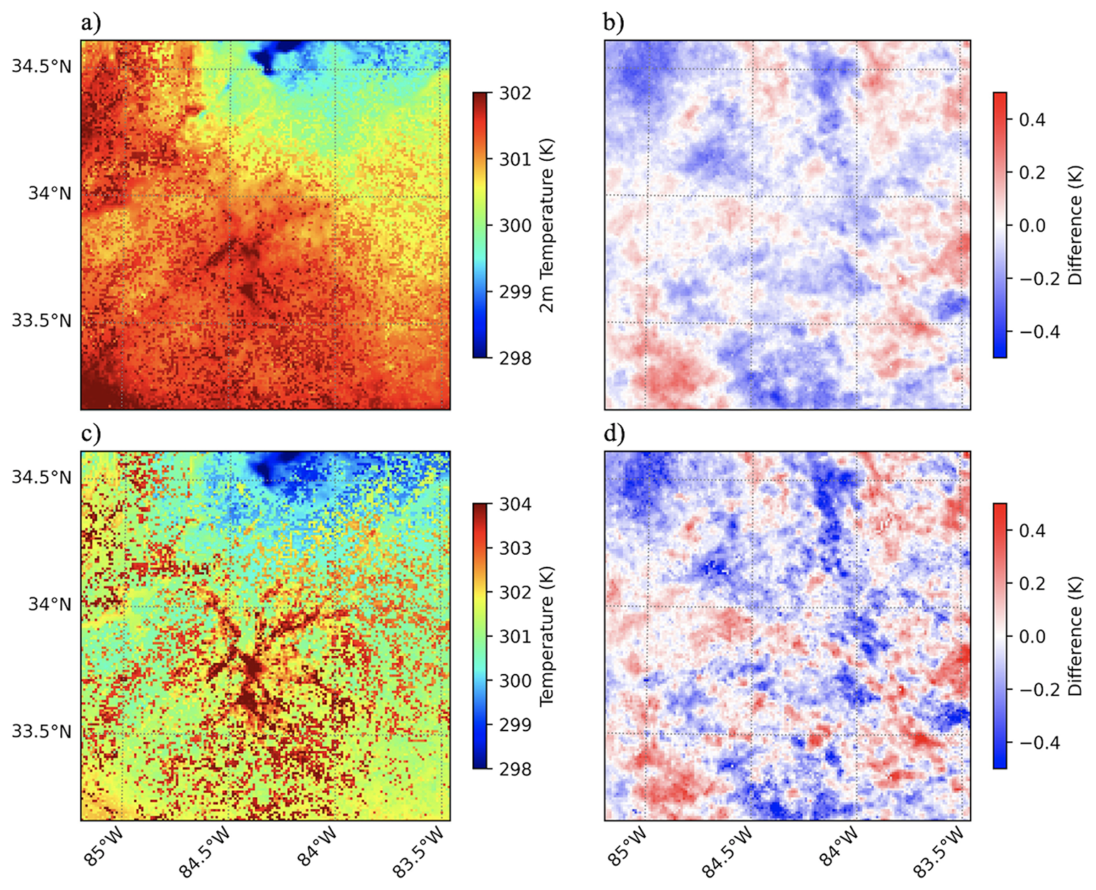
Figure A2 Panels (a) and (b) depict the average 2 m air temperature without bug fix and the 2 m air temperature difference between the cases studies with and without bug fixes implemented, respectively. Similarly, panels (c) and (d) represent the skin surface temperature output from WRF-BEP+BEM model without bug fixes implemented and the skin surface temperature difference between the case studies with and without bug fix. Panels (a)–(d) corresponds with the WRF model output for the BEP+BEM urban canopy model.

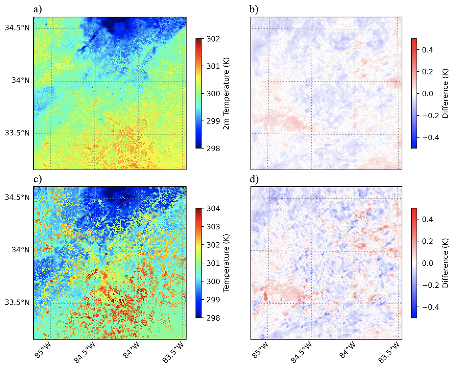
Figure A3 Panels (a) and (b) depict the average 2 m air temperature without bug fix and the 2 m air temperature difference between the cases studies with and without bug fixes implemented, respectively. Similarly, panels (c) and (d) represent the skin surface temperature output from WRF-SLUCM model without bug fixes implemented and the skin surface temperature difference between the case studies with and without bug fix. Panels (a)–(d) corresponds with the WRF model output for the SLUCM urban canopy model.