Evaluation of a coupled ocean and sea-ice model (MOM6-NEP10k) over the Bering Sea and its sensitivity to turbulence decay scales

Understanding and predicting the ocean environment and marine ecosystem status depends on accurate representations of regional ocean dynamics. Recently, the Modular Ocean Model version 6 (MOM6) has been configured to span the Northeast Pacific Ocean from Baja California to the Chukchi Sea (MOM6-NEP). In this study we present a physical hindcast (1993–2018) simulation of MOM6-NEP where it is coupled to a thermodynamic-dynamic sea-ice module and includes tides. We evaluate the performance of this model in the Bering Sea. Various model metrics are benchmarked against in-situ mooring data and satellite observations. The simulation captures the general characteristics of Bering Sea dynamics, particularly with respect to seasonal and interannual variability of the middle shelf water mass properties. Modeling of shear induced mixing was found to be critical to the model's ability to reproduce the observed sharp summer thermocline and its depth. The hindcast simulation reproduces the long-term mean timing of sea-ice arrival and retreat in both the northern and southern Bering Sea, with the remaining mild biases primarily occurring in May over the northern shelf – the model captures the mean timing of sea-ice retreat, though it tends to retreat earlier in colder years and later in warmer years compared to observations. This pattern in biases suggests that the melting rate in the model likely underestimates the well-known melt-rate dependency on ice property whereby thicker (thinner) ice melts more slowly (quickly). As a result of high skills in reproducing sea-ice areal coverage, the interannual variability of the cold pool (the cold-water mass present on the bottom of the Bering Sea shelf in summer) extent is accurately reproduced by the model. Skillful representation of sea ice and the cold pool is essential for understanding ecosystem dynamics and successful fisheries management in the Bering Sea. The findings of this study contribute to the development of reliable oceanographic modeling and forecasting of marine ecosystem conditions to support fisheries management decision making.

1 Introduction

The Bering Sea is one of the world's most productive marine ecosystems with abundant populations of fishes, birds, and marine mammals. More than 10 % of the world's fish and shellfish and about 60 % of the US commercial seafood harvest come from these ecosystems (National Marine Fisheries Service, 2024; Alaska Seafood Marketing Institute, 2023). In addition, subsistence harvests are important for the livelihoods and cultures of many families and communities in Alaska. Each year, approximately 36.9 million pounds of foods are harvested by rural communities (National Marine Fisheries Service, 2024). The significance of the productivity of the Bering Sea extends beyond the United States to the economics of its neighboring countries, including Canada and Russia.

The Bering Sea is a semi-enclosed sea (Fig. 1). To the south, the Aleutian Islands form a porous boundary between the Gulf of Alaska and the Bering Sea, and to the north, the Bering Sea is connected to the Arctic Ocean via the narrow (∼ 85 km), shallow (30–50 m) Bering Strait, which is the only source of Pacific water into the Arctic Ocean. The Bering Sea is divided almost equally between the broad (∼ 500 km wide) eastern shelf and the deep basin. The eastern Bering Sea shelf is bisected north–south at ∼ 60° N, with the southern shelf ecosystem being more pelagic and the northern shelf more benthic (Stabeno et al., 2012a). There are three cross shelf domains that are evident in summer: the coastal or inner shelf domain (0–50 m deep), which is only weakly stratified; the middle domain (50–100 m), which is strongly stratified with a well-mixed surface layer and tidally mixed bottom layer; and the outer domain (100–180 m), which is more gradually stratified in its vertical structure (Coachman, 1986; Stabeno, 1999). These domains are most clearly expressed on the southern shelf, where tidal currents are roughly twice as strong as in the north, but similar cross-shelf structures extend from the Alaska Peninsula to St. Lawrence Island, a distance of ∼ 1000 km.

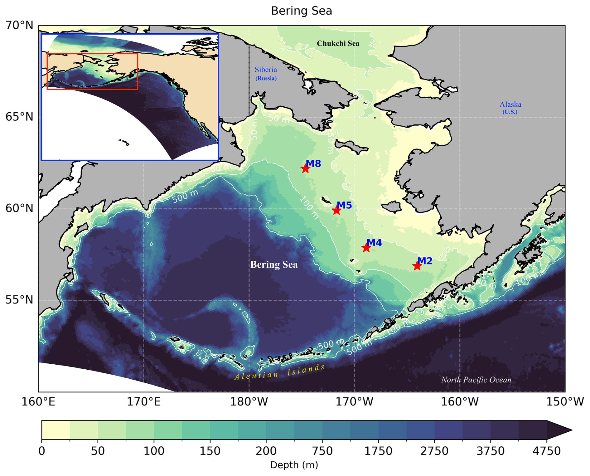
Figure 1 Study region (Bering Sea) with locations of biophysical moorings M2, M4, M5 and M8 shown by the red stars. The entire model domain is shown in the upper left-hand corner.

Well defined flow patterns exist in both the basin and over the shelf (Fig. 2a). Gulf of Alaska water enters the Bering Sea primarily through the eastern and central Aleutian Passes and exits into the North Pacific through the western passes. Flow on the eastern shelf is generally northward, in several well-defined currents (Fig. 2a). Bering Sea water also flows northward through Bering Strait into the Arctic Ocean. The Bering Sea circulation has strong seasonal variability, driven by the Aleutian Low and Siberian High atmospheric pressure systems (Danielson et al., 2011; Frey et al., 2015; Zhang et al., 2010). The strong northeasterly winds in winter, with a mean speed of ∼ 9 m s⁻¹ (Danielson et al., 2014; Stabeno and Bell, 2019), carry cold air from the Arctic, resulting in the formation of sea ice in the polynyas. In the summer, the southwesterly wind brings warm air from the south to the Bering Sea, which contributes to sea-ice retreat and melting (Woodgate et al., 2010). Interannual variability of sea ice on the Bering Sea shelf is also influenced by fluctuations of ocean transport and the associated heat and freshwater fluxes through the porous Aleutian Islands (Stabeno and Cheng, personal communication, 2025) and Bering Strait (Woodgate et al., 2006; Woodgate et al., 2012). Sea ice is a critical component of the Bering Sea ecosystem. It sets up the “cold pool”, a layer of cold (traditionally defined as < 2 °C) bottom water over the eastern shelf that can persist through the summer. The extent of the cold pool affects species distribution. In addition, the timing of sea-ice melt influences the timing of the spring phytoplankton bloom (Hunt et al., 2002, 2011).

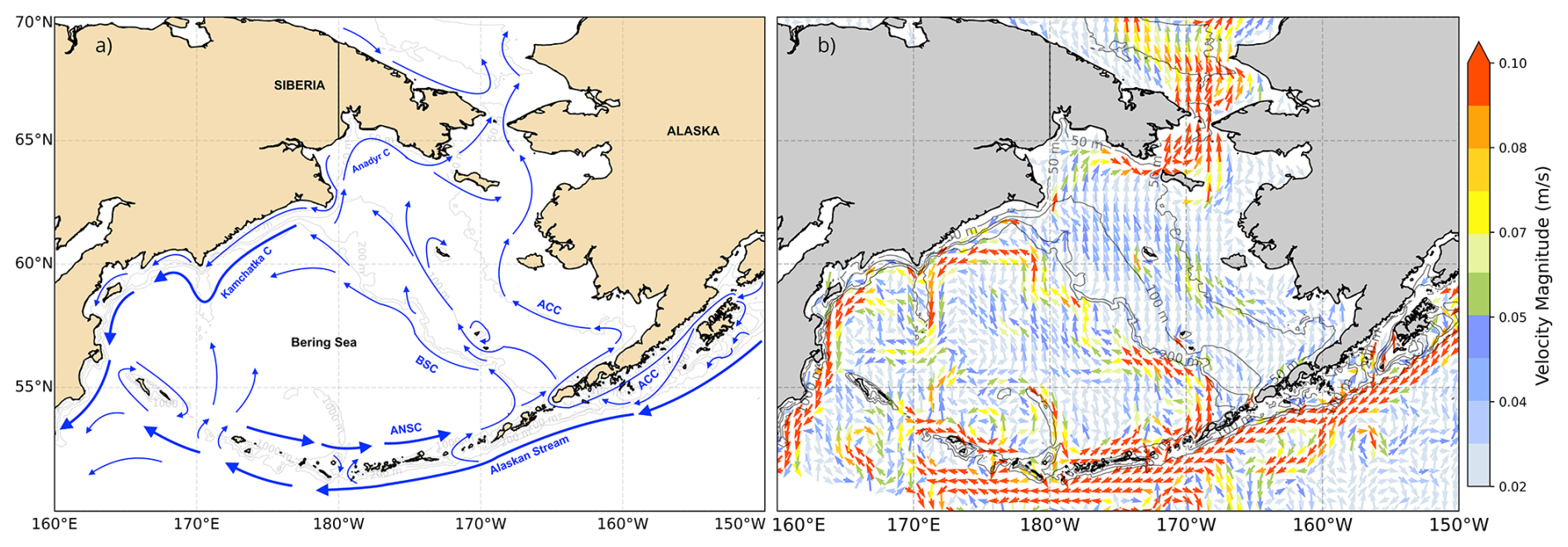
Figure 2 (a) A schematic of the flow patterns in the Bering Sea and along the Aleutian Islands (adapted from Stabeno, 1999; Stabeno et al., 2005). Abbreviations: ANSC is Aleutian North Slope Current; BSC is Bering Slope Current; and the ACC is the Alaskan Coastal Current. (b) Annual mean current in 2016 at 20 m depth from MOM6-NEP10k. Vectors represent the current direction and color indicates the speed.

Over the past several decades, extensive oceanographic and fisheries observations have been conducted in this rich ecosystem. Measurements include shipboard conductivity-temperature-depth (CTD) casts, biophysical moorings (Stabeno et al., 2023; Cokelet and Stabeno, 1997; Onishi and Ohtani, 1999), shipboard and moored ADCP (Acoustic Doppler Current Profiler) current meters (Cokelet et al., 1996; Stabeno et al., 2016), and satellite-tracked drifters (Stabeno and Reed, 1994). While these observations reveal structure and dynamics of the Bering Sea, they are limited in time and space, providing an incomplete picture of the relationship among physical, chemical and biological processes. Coupled ocean/sea-ice simulations are necessary to gain a better understanding of the Bering Sea and to predict its changes on seasonal, interannual and multidecadal time scales which are driven by natural variability and human activities. These predictions can provide information to help decision makers to better manage marine fisheries and inform local communities who depend on these marine ecosystems.

Recently, a new regional ocean model configuration has been developed stretching from the Baja Peninsula through the Bering Sea and into the Chukchi Sea (Drenkard et al., 2025). It is based on the Modular Ocean Model version 6 (MOM6; Adcroft et al., 2019), which plays a growing role in regional ocean modeling across National Oceanic and Atmospheric Administration (NOAA) line offices. This configuration, which focuses on the Northeast Pacific (MOM6-NEP), captures numerous fisheries-critical physical and biogeochemical features across the disparate marine ecosystems encompassed by this large domain with fair to high skill. The Bering Sea, however, has proved particularly challenging due to its extraordinary range of bathymetric features, dynamic circulation, and atmosphere/ocean/sea-ice interactions. Together with the outsized importance of the Bering Sea ecosystem for commercial and subsistence fisheries, this provides a compelling impetus for a more detailed evaluation of the model performance in this region.

During the last 20 years, hydrodynamical modeling of the Bering Sea has been primarily based on the Regional Ocean Modeling System (ROMS). Hermann et al. (2013, 2019, 2021) used coupled physical–biological models, incorporating benthic components, to examine lower trophic level dynamics and ecosystem responses to climate variability. Kearney et al. (2020) used a high-resolution configuration of ROMS to explore the drivers of ocean temperature and sea-ice variability across the shelf. Simulations from these efforts revealed strong linkages between physical forcing and key ecosystem components such as large crustacean zooplankton. More recent studies have extended the scope of Bering Sea modeling toward climate downscaling and scenario projections, using coupled physical–biogeochemical models based on ROMS frameworks (Cheng et al., 2021; Hermann et al., 2021; Pilcher et al., 2022).

In this paper, we performed hindcasts (using MOM6-NEP) during 1993–2018 under historical atmospheric and oceanic lateral boundary conditions. First, to address excessive shear-driven vertical mixing found in the MOM6-NEP default configuration (Fig. S2 in the Supplement), we implemented a non-dimensional scaling factor to the turbulent mixing decay length scale and examined sensitivity of the simulated water mass characteristics to this factor (see Sect. 3.1). Using this new scaling factor, we then focused on three components of model output: general circulation; sea-ice timing and extent; and water column stratification. We evaluated this output against long-term bio-physical mooring data (Stabeno et al., 2023), satellite observations (sea surface temperature, sea-ice extent, sea surface height, etc.), and mixed layer depth based on World Ocean Atlas and ARGO datasets.

2 Methods and Datasets

2.1 Model Description

MOM6 incorporates many improvements compared to its predecessor, MOM5 (Griffies, 2012), including: the incorporation of the Arbitrary Lagrangian Eulerian (ALE) vertical coordinate (Bleck, 2002; Griffies et al., 2020); the implementation of tracer advection schemes that are more efficient; and state-of-the-art parameterizations of sub-grid scale physics. These new parameterizations include energetically constrained surface boundary layer dynamics (Reichl and Hallberg, 2018), mesoscale thickness mixing (Jansen et al., 2015), sub-mesoscale mixed layer re-stratification (Fox-Kemper et al., 2011), and shear-driven turbulence mixing in the interior ocean (Jackson et al., 2008). MOM6 is coupled with a dynamic and thermodynamic sea-ice model Sea Ice Simulator 2 (SIS2) (Adcroft et al., 2019). Currently, open lateral boundary conditions for sea ice are not implemented in MOM6-NEP. Since the primary region of interest in this study, the Bering Sea, is ∼ 1200 km away from the model's lateral boundary and sea ice in the Bering Sea is formed mostly locally, treatment of sea-ice boundary conditions is not expected to affect our results significantly.

As described in Drenkard et al. (2025), the horizontal grid of MOM6-NEP is based on an Arakawa C grid (Arakawa and Lamb, 1977), and has a resolution of ∼ $\mathrm{1}/\mathrm{10}$° (∼ 9.7 km ± 0.5 km) with 342 × 816 tracer points. Horizontally, the model uses an orthogonal curvilinear grid and extends from 10.8 to 80.7° N and 156.6° E to 105.0° W (Fig. 1). In the vertical, a 75 layer z^* remap coordinate (Adcroft and Campin, 2004) is used. The layer thickness is 2 m near the surface, gradually increasing to 250 m at the deepest model depth of 6500 m. The shallowest bathymetry in the model is 5 m (i.e., areas where the true bathymetry is less than 5 m deep are set to 5 m). The domain has four open boundaries, the longest of which arcs through the Pacific Ocean and is here referred to as the “western” boundary as it is adjacent to the northwestern Pacific.

MOM6-NEP is integrated forward in time with a split explicit method (Hallberg, 1997; Hallberg and Adcroft, 2009). It uses a variable barotropic timestep set to maintain stability, a baroclinic time step of 600 s, and a thermodynamic time step of 1200 s to increase computational efficiency (e.g., Ross et al., 2023; Drenkard et al., 2025). Oceanic and atmospheric data sets used to force MOM6-NEP in this study are described in Sect. 2.2.

2.2 Model Forcings

Initial and ocean open boundary conditions are specified using the high resolution ($\mathrm{1}/\mathrm{12}$°) Global Ocean Physics Reanalysis (GLORYS12v1; Jean-Michel et al., 2021), which includes daily averages of 3-D ocean temperature, salinity, sea-surface height (SSH), meridional (v) and zonal (u) velocity components. GLORYS12 is one of the better-performing ocean reanalyses in coastal areas (Castillo-Trujillo et al., 2023; Amaya et al., 2023). In Amaya et al. (2023), GLORYS12 was shown to have sea surface temperature (SST) Root Mean Square Error (RMSE) values of ∼ 0.25–0.6 °C and monthly SST anomaly correlations > 0.9 at nearshore locations along the west coast. Tidal forcing was obtained from the TPXO9 v1 model (Egbert et al., 2002). Ten tidal constituents are specified at the boundaries as was done in Ross et al. (2023) and Drenkard et al. (2025), including four semidiurnal constituents (M2, S2, N2, and K2), four diurnal constituents (K1, O1, P1, and Q1), and two long-period constituents (Mm and Mf).

The barotropic flow at the open boundaries is treated with a Flather boundary condition (Flather, 1976), and the baroclinic component is specified using the Orlanski boundary condition (Orlanski, 1976). The boundary flows are nudged to exterior velocities at timescales of 3 d for inflow and 360 d for outflow (Marchesiello et al., 2001). Nudging layers for temperature, salinity and velocities are applied to minimize noise at the boundaries that may contaminate the interior. River discharge is obtained from the Global Flood Awareness System version 3.1 (GloFAS, Zsoter, 2021). The full implementation is described in Drenkard et al. (2025).

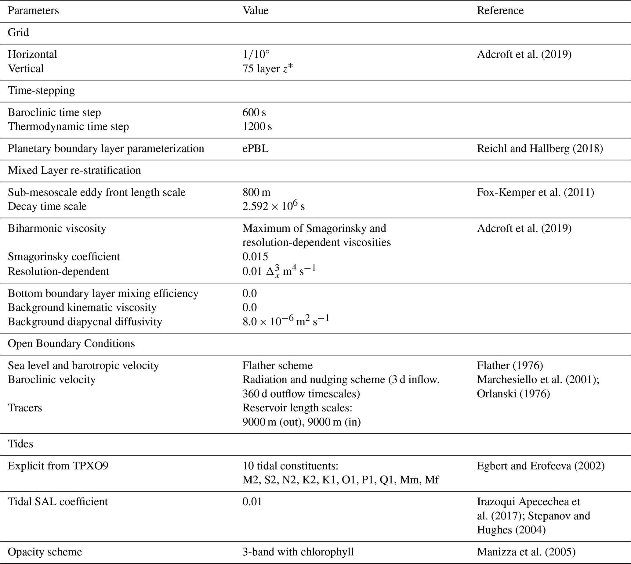
In our study we used the 3 h Japanese 55-year Reanalysis (JRA55) (Kobayashi et al., 2015) for atmospheric forcing, whereas Drenkard et al. (2025) used 1 h ECMWF reanalysis v5 (ERA5) for this purpose. The JRA55 forcing variables include downward shortwave and longwave radiative fluxes, precipitation (separated into rain and snow), zonal and meridional winds, sea level pressure, air temperature and specific humidity. We used the JRA55-do version 1.5 (Tsujino et al., 2018), which is specifically designed for ocean–ice modeling applications. It provides consistent atmospheric variables for bulk flux calculations, applies bias corrections to prevent artificial trends, and is compatible with CORE/OMIP forcing protocols. The bulk formulae of Large and Yeager (2004) were used to calculate surface buoyancy and momentum fluxes as a function of modeled SST and ice concentration, and specified atmospheric forcing variables. Light attenuation within the water column is calculated following the Manizza et al. (2005) opacity scheme, which is influenced by monthly climatology of surface chlorophyll a (Chl a) concentration from the SeaWiFS satellite mission (NASA Ocean Biology Processing Group, 2018). Table 1 provides a summary of MOM6-NEP configuration, parameterization schemes, and parameter values used in this study, and relevant references.

Table 1 Base model configuration, parameterization schemes and associated parameter values, and relevant references.

2.3 Evaluation datasets

The Optimum Interpolation Sea Surface Temperature (OISST) dataset (Huang et al., 2021) with spatial resolution of 0.25° × 0.25° is used to validate modeled SST. For sea surface salinity (SSS) evaluations, we used the northern North Pacific regional climatology version 2 (NNP RC; Seidov et al., 2023) with a spatial resolution of 0.1° × 0.1° from the NOAA National Centers for Environmental Information (NCEI). NNP RC version 2 covers a period of seven decades. MOM6-NEP SSH is compared to absolute dynamic topography (spatial resolution of 0.25° × 0.25°) obtained from the Copernicus Marine Service's (Global Ocean Gridded L4) satellite altimetry dataset (Mercator Ocean, 2021).

During integration, MOM6-NEP computes the mixed layer depth (MLD) using instantaneous vertical profiles. The MLD is defined as the depth at which modeled potential density increases by 0.03 kg m⁻³ relative to its surface value. The computed MLD are then saved as daily averages. These are compared to the long-term MLD monthly climatology (1° × 1° spatial resolution) derived from profiles in the World Ocean Database and Argo datasets (de Boyer Montégut, 2024; de Boyer Montégut et al., 2004). The MLD in this dataset is also defined as the depth at which the density is 0.03 kg m⁻³ greater than the density of the surface layer, although its surface layer is at 10 m whereas the surface layer in MOM6-NEP is at 2 m. In addition to MLD, we also calculated thermocline depth, which is where the maximum vertical temperature gradient above a threshold of 0.1 °C m⁻¹ occurs. We consider temperature gradients within the 5–70 m depth range. If the gradient is weaker than 0.1 °C m⁻¹ throughout the water column, we assign 70 m as the thermocline depth. This calculation is done using daily model output and temperature measured at mooring site M2. Daily sea-ice concentration data were retrieved from National Snow and Ice Data Center (https://nsidc.org/data/nsidc-0079/versions/4, last access: 20 November 2024 and https://nsidc.org/data/nsidc-0081/versions/2, last access: 20 November 2024).

Simulated daily bottom temperature on the Bering Sea shelf was sampled each year following the Alaska Fisheries Science Center (AFSC) Groundfish Bottom Trawl Survey; the “survey replicate” model output is then compared with bottom trawl data. Details on the bottom trawl data collection and postprocessing are described in Buckley et al. (2009) and Lauth (2011), and the data are available at https://github.com/afsc-gap-products/coldpool (last access: 15 October 2024). The cold pool spatial distribution and its interannual variability were constructed following the method described in Kearney (2021), and the same method is applied to both modeled and survey data.

2.4 Moorings

Modeled temperature and salinity are evaluated against the long-term Bering Sea biophysical mooring data along the 70 m isobath (Fig. 1; Stabeno et al., 2023). Moorings at M2 (56.87° N, 164.06° W) are deployed and recovered twice a year, once during the spring (April/May) and again in late summer or early autumn (September/October). The September/October deployment is a subsurface mooring with the uppermost instrument at 11 m. The spring deployment is a surface mooring. Moorings at M2 have been maintained since 1995 (Stabeno et al., 2010, 2023), although there are some gaps primarily due to fishing. Mooring M4 (57.9° N, 168.9° W) has been maintained since 1998, while the last two mooring sites, M5 (59.9° N, 171.7° W) and M8 (62.2° N, 174.7° W), have been maintained since 2005. M4 is typically turned around (recovered and redeployed) in the spring, while M5 and M8 are turned around in the late summer. The primary moorings are built using chain to safeguard against potential damage from sea ice and the significant fishing activity in this region. The moorings were equipped with instruments that collect a wide variety of data: temperature (miniature temperature recorders, SBE-16, SBE-37 and SBE-39), salinity (SBE-16, SBE-37), nitrate, and chlorophyll fluorescence (WET Labs DLSB ECO Fluorometer). A companion mooring at each site measures currents using a 300 or 600 kHz acoustic Doppler current profiler (ADCP).

Since 2018, the summer mooring at M2 has contained a Prawler (Profiling crawler; used in 2018), that measures temperature, salinity, fluorescence, O₂, and pressure in the upper ∼ 45 m (Stabeno et al., 2023; Stalin et al., 2023). Prior to 2018 and during the winter at M2, the vertical sampling resolution in the upper 30 m is ∼ 3 m, and in the bottom 40 m is ∼ 5 m. The winter mooring remains deployed for one year. A similar resolution occurs at M4 (upper instrument at 11 m), M5 (upper instrument at 15 m) and at M8 (upper instrument at 20 m). All instruments sample at least hourly and are calibrated prior to deployment. All data are processed in accordance with the specifications provided by the manufacturers.

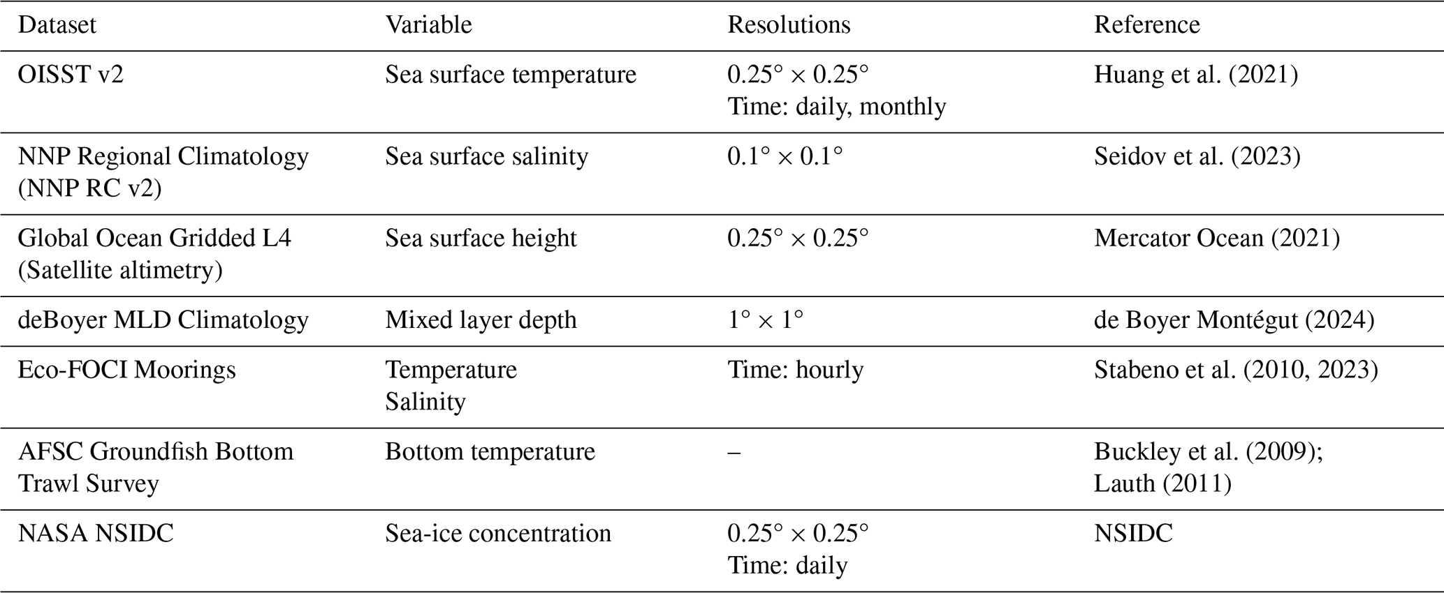
A summary of observational datasets, their resolution, and sources used to evaluate MOM6-NEP is shown in Table 2. To compare model output against different data products, we used the xesmf Python package (Zhuang et al., 2023) to bi-linearly interpolate the dataset with higher resolution onto the horizontal grid of the product with lower resolution.

Table 2 Summary datasets used for evaluation of MOM6-NEP model performance.

3 Results

3.1 Refinement of the shear-driven vertical mixing

Shear-driven vertical mixing in the interior ocean is modeled following Jackson et al. (2008). In this parameterization scheme, the turbulent kinetic energy (TKE) and diffusivity are determined by vertically nonlocal steady-state equations. The steady-state assumption is applicable in models with time steps longer than the characteristic turbulence evolution time scale. The default Jackson et al. (2008) parameterization of shear-driven turbulence was found to over-mix the Bering Sea shelf, eroding the thermocline in summer (Fig. S2); this was especially true in the southern domain which is characterized by strong tides. To account for the additional turbulent processes that disrupt the growth of shear-driven turbulence which is not captured by the default Jackson scheme, we introduced a rescaling factor, lz_rescale (β) to the formulae of decay length scale (L_d) for eddy diffusivity (κ) such that

$$\begin{array}{}\text{(1)}& L_{\mathrm{d}}=min\left(\mathit{\lambda }{L}_{\mathrm{b}},\mathit{\beta }{L}_z\right)\end{array}$$

where λ is a non-dimensional scaling factor, L_b is the buoyancy length scale, and L_z is the distance to the nearest vertical boundary. In the original formulation, β is 1, resulting in the unmodified contribution of L_z to L_d.

We tested different values of λ and β, along with perturbations to several other model parameters (C_N, C_S, and Ri_c) in a suite of sensitivity tests. C_N and C_S are non-dimensional turbulent kinetic energy dissipation coefficients associated with stratification and shear, respectively, while Ri_c is the critical Richardson number above which turbulent mixing does not occur. Our perturbed values of these parameters are within the bounds of theoretical arguments (Jackson et al., 2008). We also turned off tidal forcing in one sensitivity test. The vertical profiles of shear-driven diapycnal diffusivity from the sensitivity tests and the control simulation (CTRL) are shown in Fig. 3. CTRL exhibits strong shear-driven vertical diffusivity throughout the water column with a local maximum around 50 m, and its magnitude (∼ 3.5 × 10⁻² m² s⁻) is approximately 7–8 times bigger than shear-driven mixing in the surface boundary layer. While direct microstructure measurement of eddy diffusivity, which has strong heterogeneity both vertically and horizontally, is limited, this amplitude of shear-driven mixing is larger than observed values in the global oceans (Itoh et al., 2021). With this strong mixing, the modeled water column at M4 is well mixed even in summer, missing the well-defined thermocline in observations. Such strong mixing has significant implications for nutrient dynamics and biological processes. The “No-Tides” run suggests that this over-mixing is strongly coupled to tidal dynamics in the bottom boundary layer. Increasing Ri_c promotes even more mixing, consistent with dynamical understanding of the critical Richardson number. Increasing dissipation through larger C_N and C_S (than in CTRL) results in a limited decrease in mixing. Changing both λ and β (green dotted and purple dashed lines, Fig. 3) achieves similar effects to perturbing β alone (red and olive solid lines, Fig. 3).

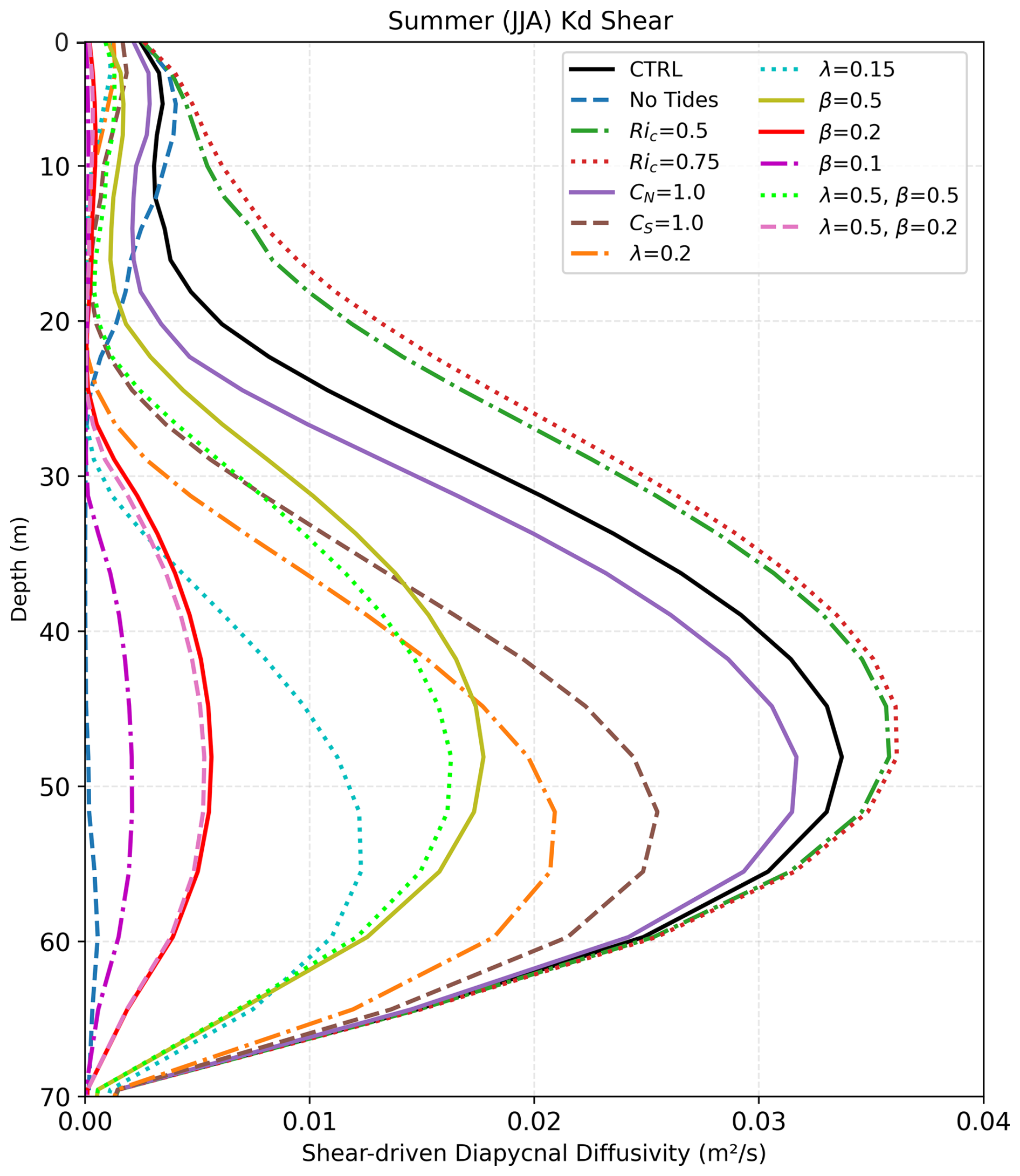
Figure 3 Vertical profiles of shear-driven vertical mixing coefficient in the summer (June-July-August average) of 2000 at the M4 location from the control simulation (CTRL, black solid line) and the sensitivity tests (colored lines). In each of the sensitivity tests, only the parameters specified in the line legend are perturbed, while all other parameters remain unchanged from CTRL.

The effects of these perturbations on the modeled summer bottom temperatures at the mooring locations and their comparisons with observations are summarized by a Taylor diagram (Fig. 4). Across all mooring locations, experiment β= 0.2 (represented by the red square) consistently maintains its proximity to the OBS point (Fig. 4a–d), showing low RMSE relative to OBS, nearly perfect reproduction of the observed interannual variability, and strong correlation with OBS (R>0.92). The maximum shear-induced diffusivity at 50 m in experiment β= 0.2 is reduced to 5 × 10⁻³ m² s⁻¹, bringing it into better alignment with observations. In contrast, CTRL (black star) and experiments Ri_c= 0.5 and Ri_c= 0.75 (green and red hexagon, respectively) show significant deviations from OBS. Other sensitivity tests (with the exception of the “No Tides” experiment) generally fall between the CTRL and β= 0.2. The “No-Tides” experiment shows much weaker interannual variability of bottom temperature than OBS and other sensitivity experiments, highlighting the importance of tides, tidally induced mixing and its interactions with other oceanic processes.

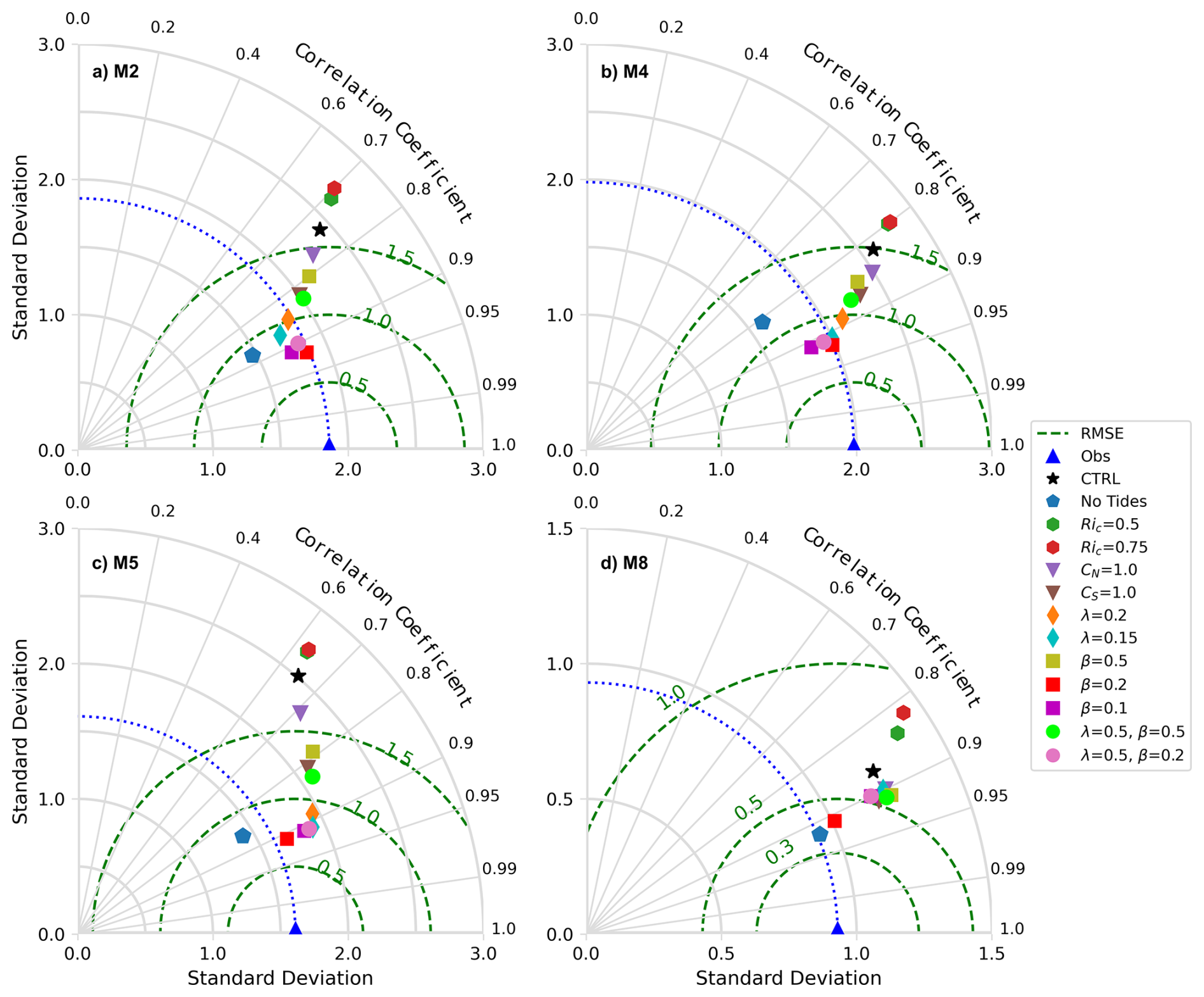
Figure 4 Taylor diagram showing the standard deviation of both modeled and observed bottom temperature, along with correlation coefficients and RMSEs between the modeled and observed bottom temperature at the mooring locations (a) M2, (b) M4, (c) M5, and (d) M8. Results from OBS, CTRL, and sensitivity tests are represented by distinct symbols, with the symbol legend displayed on the right. Note that the x and y axis scales in panel (d) are half of those in the other panels. These statistics were calculated using the monthly means of bottom temperature from the respective mooring periods (M2: 1995–2018, M4: 2000–2018, M5: 2005–2018, M8: 2005–2018).

In addition to the point-wise comparison, we also examined the modeled shelf-wide bottom temperature against the annual AFSC bottom trawl survey. In this evaluation, daily temperatures from the model are first subsampled in time and horizontal locations following the survey data, generating survey-replications of the model output. Figure 5 shows scattered plots between survey and survey-replicated model output from CTRL and the best fit experiment β= 0.2 (Fig. 4) over the hindcast period (1993–2018). Experiment β= 0.2 shows a tighter correspondence with observations than CTRL, having reduced bias (0.42 to 0.24 °C) and RMSE (1.33 to 0.97 °C), and a higher correlation coefficient (0.82 to 0.90). These results indicate that limiting shear-driven vertical mixing through lz_rescale improves the model's capacity to replicate bottom temperature dynamics, particularly under Bering Sea tides (∼ 30 cm s⁻¹). Interestingly, observed temperatures in the warmest range (> 13 °C) that occurred primarily in 2016–2018 (yellow) tend to be cooler than the modeled temperatures in the same years. This will be further explored in Sect. 3.4.

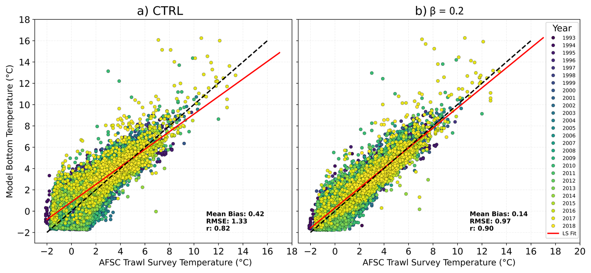
Figure 5 Scatter plots of temperature from the AFSC bottom trawl survey (x axis) versus modeled survey-replicated bottom temperature (y axis) from (a) CTRL and (b) the β= 0.2 experiment. Data point colors represent different years. The red lines represent the least square fits, while the black dashed lines indicate the 1:1 relationship.

Since experiment β= 0.2 provides the overall best fit with observations, this parameterization is used in all ensuing analyses. We refer to this particular model configuration as MOM6-NEP10k v1.1P, where P stands for “physics only”. The main differences between MOM6-NEP10k v1.1P and MOM6-COBALT-NEP10k v1.0 (Drenkard et al., 2025) are: (1) MOM6-COBALT-NEP10k v1.0 is coupled to marine biogeochemical processes (the internally generated phytoplankton influence shortwave absorption) whereas MOM6-NEP10k v1.1P is physics only (a satellite-derived phytoplankton climatology is imposed); (2) atmospheric forcing in MOM6-NEP10k v1.1P is JRA55 while in MOM6-COBALT-NEP10k v1.0 it is ERA5; (3) MOM6-COBALT-NEP10k v1.0 uses the Bodner scheme (Bodner et al., 2023) where mixed layer submesoscale frontal length is calculated dynamically whereas in MOM6-NEP10k v1.1P it is specified as a constant (800 m).

3.2 Circulation

MOM6-NEP10k v1.1P replicates the main current systems in the northern Gulf of Alaska and Bering Sea (Fig. 2a). In the Gulf of Alaska, the Alaskan Stream, the southwestward flowing western boundary current of the eastern Subarctic Gyre (Stabeno and Hristova, 2014), is clearly evident (Fig. 2b). Over half of this transport flows through the deeper passes (e.g., Amukta Pass, Amchitka Pass, and Near Strait) to form the Bering Sea Gyre (Stabeno et al., 2005; Stabeno, 1999; Reed and Stabeno, 1993). Each branch of the Bering Sea Gyre (Aleutian North Slope Current, Stabeno et al., 2009; Reed and Stabeno, 1999, the Bering Slope Current, Ladd, 2014, and the Kamchatka Current, Stabeno et al., 1994) is well-represented in the model simulations (Fig. 2a, b).

The flow on the broad, eastern shelf is generally northward (Fig. 2a). Once again, the model replicates the current systems (Fig. 2b). There are two well defined currents on the eastern shelf (Stabeno et al., 2016): the Alaska Coastal Current (ACC) which flows northward along the 50 m isobath (the boundary between coastal domain and middle shelf domain) and northward flow along the 100 m isobath. The ACC eventually flows through the eastern side of the Bering Strait. The flow along 100 m isobath joins with the Anadyr Current which flows eastward along the southern side of the Siberian coast and enters the Arctic through the western side of Bering Strait.

The magnitude of flow through the Aleutian Passes is critical for the transport of heat and salts northward into the Bering Sea. In addition, the only source of Pacific water into the Arctic is through the Bering Strait. A careful comparison of the magnitude of transport through the passes is beyond the scope of this paper and will be explored in a later manuscript.

3.3 Sea-ice extent and seasonal timing

Sea ice structures the Bering Sea shelf, from ocean temperature to timing of the spring bloom to the range of fish species. While the eastern Bering Sea (here defined as the region north of Aleutian Islands, south of 66° N, and east of 178° E) is ice free in the summer, maximum areal ice extent in winter varies among years, ranging from < 0.4 × 10⁶ km² in warm years to 1.0 × 10⁶ km in cold years (Fig. 6b, c). In the satellite-era, the largest ice extent occurred in 2012 when it covered almost the entire eastern shelf, while the smallest extent occurred in 2018, when ice was largely confined to the northern shelf (Fig. 6a, purple and blue lines; the March dates used for comparison were selected based on satellite observational data as reported in Stabeno and Bell, 2019). This warm-to-cold year contrast is well captured by the model (Fig. 6). The long-term (1993–2018) mean ± standard deviation of areal ice extent in March (the month with maximum ice) is 0.65 ± 0.14 × 10⁶ km² in MOM6-NEP (coefficient of variation, CV = 21.5 %) and 0.71 ± 0.14 × 10⁶ km² in satellite observations (CV = 19.7 %). These similar CV values suggest comparable relative interannual variability in both datasets.

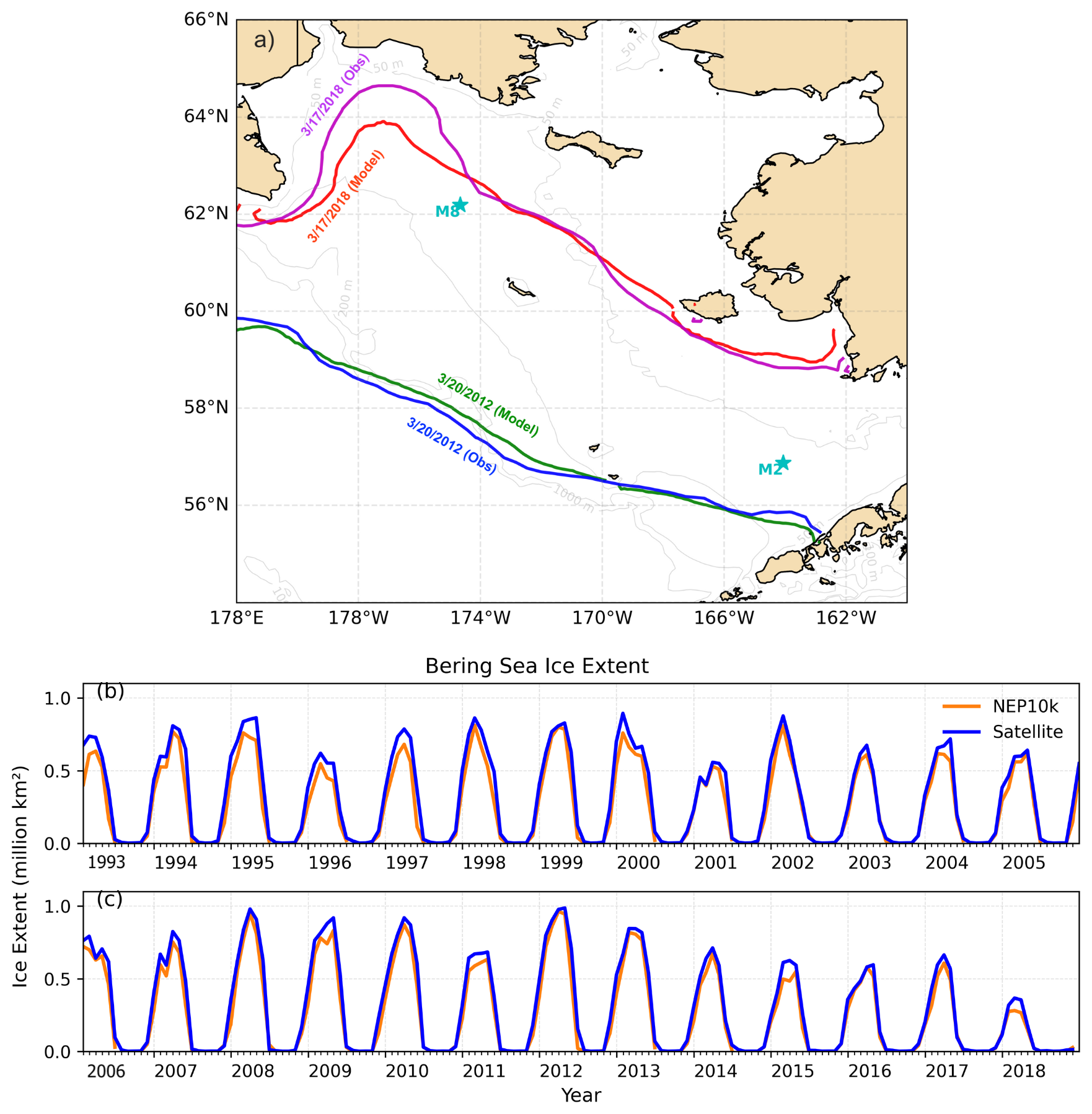
Figure 6 (a) Ice edge defined by the 10 % ice concentration in two extreme years, 2012 and 2018. (b, c) Monthly mean areal sea-ice extent over the Bering Sea from MOM6-NEP10K (orange line) and satellite observations (blue line). Ice extent is defined as the total area of grid points with ≥ 10 % ice cover. The satellite data was obtained from the National Snow and Ice Data Center, using the “climate data record” monthly ice concentration at 25 km × 25 km horizontal resolution.

Modeled sea-ice cover at the mooring locations is further evaluated against satellite observations. At M2, there is large interannual variability in sea ice (Fig. 7a, b). Since 2000 there have been a series of cold years with extensive sea ice (e.g., 2007–2013), and warm years with little/no ice reaching the southern shelf (2001–2005 and 2014–2022) (Stabeno et al., 2023). At M8, sea ice is far more persistent, but even here there are years with more persistent sea ice (e.g., 2006–2013, excluding 2011). MOM6-NEP not only replicates the areal ice coverage in the entire Bering Sea (Fig. 6), but also reproduces both seasonal and interannual variability at M2 and M8 (Fig. 7).

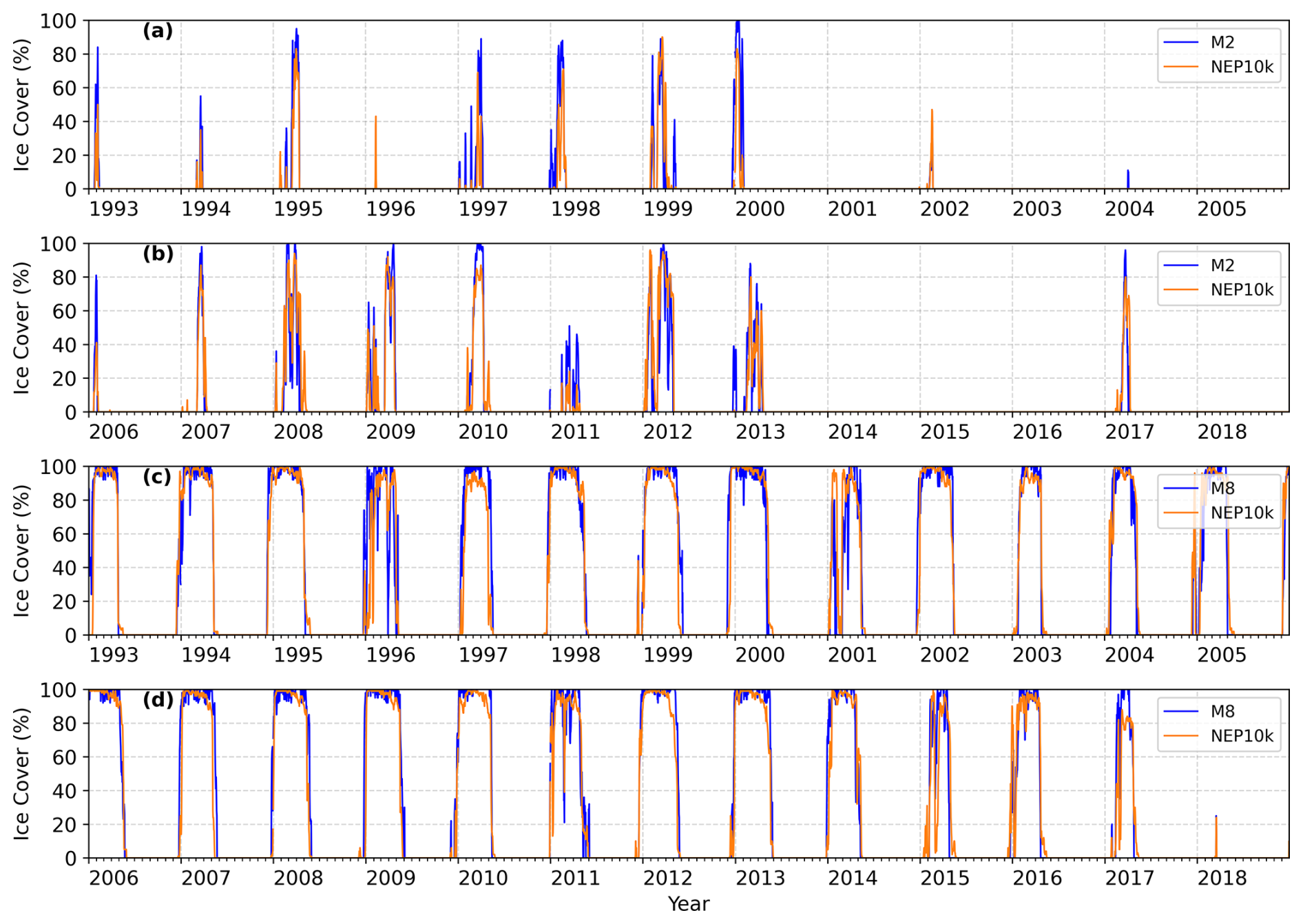
Figure 7 The averaged ice cover (percentage) in a 25 km × 25 km box centered on the mooring sites from MOM6-NEP10K (orange line) and satellite observation (blue line) at (a, b) M2 and (c, d) M8.

A more detailed examination of the difference between modeled and observed daily ice concentration at the mooring sites (Fig. 8) reveals striking patterns. First, the mean seasonal signal from observations is replicated by the model at both M2 (Fig. 8b) and M8 (Fig. 8d), where the timing of modeled ice arrival and retreat closely matches the observed timings, although the model tends to underestimate sea-ice cover at these locations by a small amount at the beginning and at the end of the ice season. This agreement in the timing of seasonal ice advance and retreat is a notable improvement from previous studies using global or regional models (e.g., Cheng et al., 2014; Kearney et al., 2020).

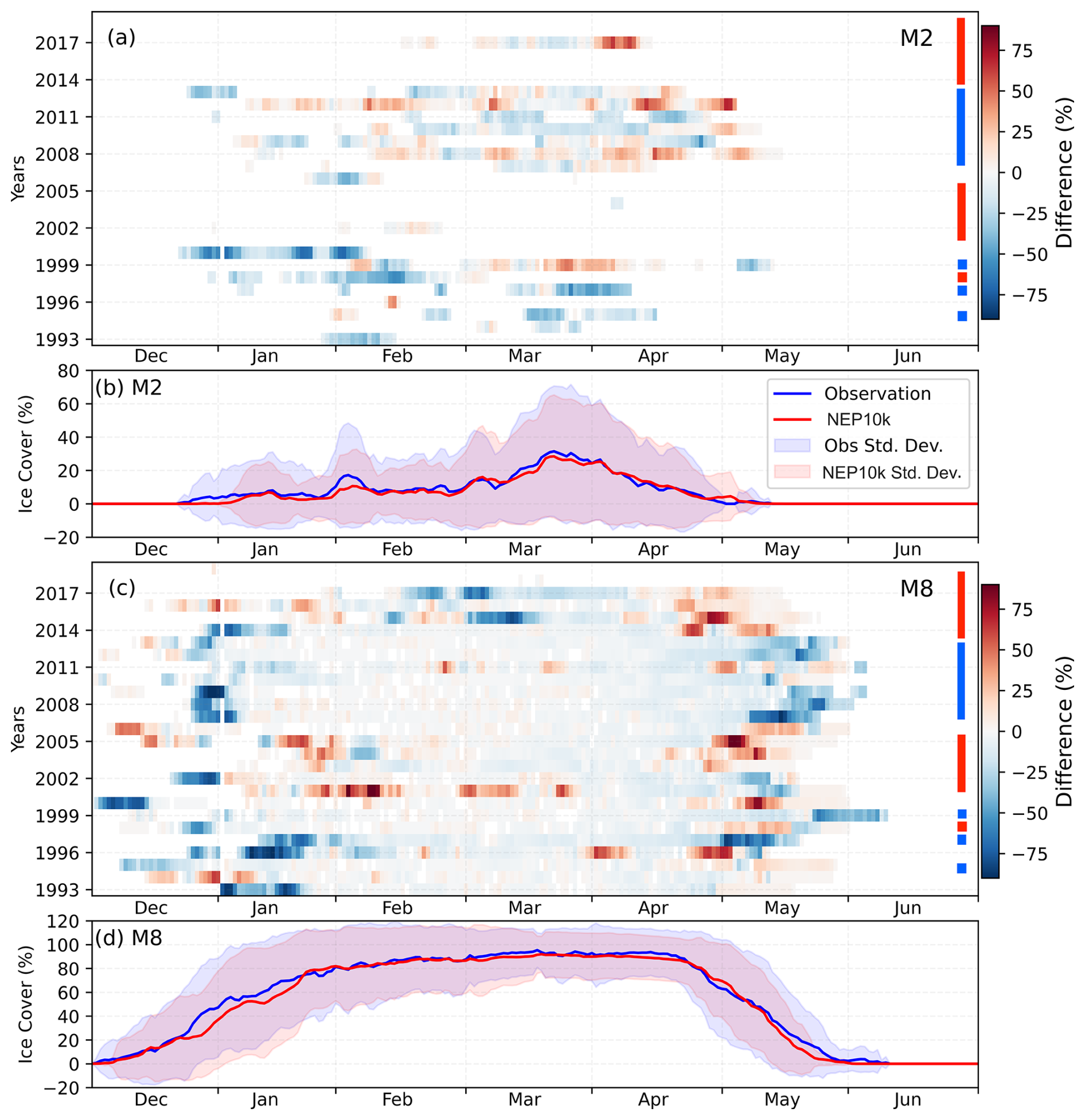
Figure 8 Difference between modeled and observed daily ice concentration (modeled minus observation) at mooring locations (a) M2 and (c) M8. Climatology (averaged over 1993–2018) of observed (blue line) and modeled (red line) daily ice concentration at (b) M2 and (d) M8; shading represents one standard deviation of the interannual variability. Blue and red vertical bars (near the right y axis) on (a) and (c) correspond to anomalously cold and warm periods, respectively (Stabeno et al., 2012b, 2023).

At both mooring sites, the greatest discrepancies are during ice formation (December-early January) and ice melt (typically April at M2 and May at M8) (Fig. 8a, c). The discrepancy (model minus observed daily sea ice concentration) at M2 is smaller than at M8. This is particularly true during 2001–2005, 2014–2016 and 2018. This is not surprising, since sea ice did not penetrate into the southern shelf during these years, and this lack of ice was replicated in the model output (Fig. 8a). At M8 discrepancies occurred throughout the study period, except 2018 when there was no ice at M8 (Stabeno and Bell, 2019). One pattern that persists is that in years with more ice (e.g., 1999, 2007–2013), the simulation tends to have earlier than observed ice retreat (represented by the negative discrepancies), whereas in years with less ice (e.g., 2001–2005, 2014–2018), modeled ice concentration at the M8 location tends to have later than observed ice retreat (represented by the positive discrepancies).

One possible explanation for this pattern is that the model melts all ice at more even rates than observations. It is well known that thicker ice melts more slowly than thinner ice (Thorndike et al., 1975). While SIS2 uses a multi-category ice thickness scheme and differentiates melt rates for different ice categories (Adcroft et al., 2019), some biases still arise due to unresolved processes such as melt pond formation, snow effects, or errors in atmospheric forcing. Thus, it underestimates more subtle differences in the complexity of ice melt, and appears to melt thin/less ice too slowly and thick/more ice too fast, resulting in the noted discrepancy. M2 does not show this systematic bias pattern because it is mostly young ice. In addition, ice on the southern shelf can be influenced by wind forced advection (retreat) in addition to just local melting (Stabeno et al., 2012a). Addressing these processes may improve model performance in future configurations.

3.4 Sea surface temperature and salinity, mixed layer depth, and sea surface height

Both the modeled and OISST mean SST (Fig. 9a, b) show strong gradients oriented roughly parallel to the shelf break. Overall, simulations were cooler on the shelf, but warmer in the deeper basin (Fig. 9c). The largest cold biases were in the Chukchi Sea, and were primarily caused by biases in the summer months (Fig. 10c). This may be partly due to the absence of sea-ice open boundary conditions, which can lead to excessive sea-ice retention and surface cooling by limiting ice exchange across the northern boundary.

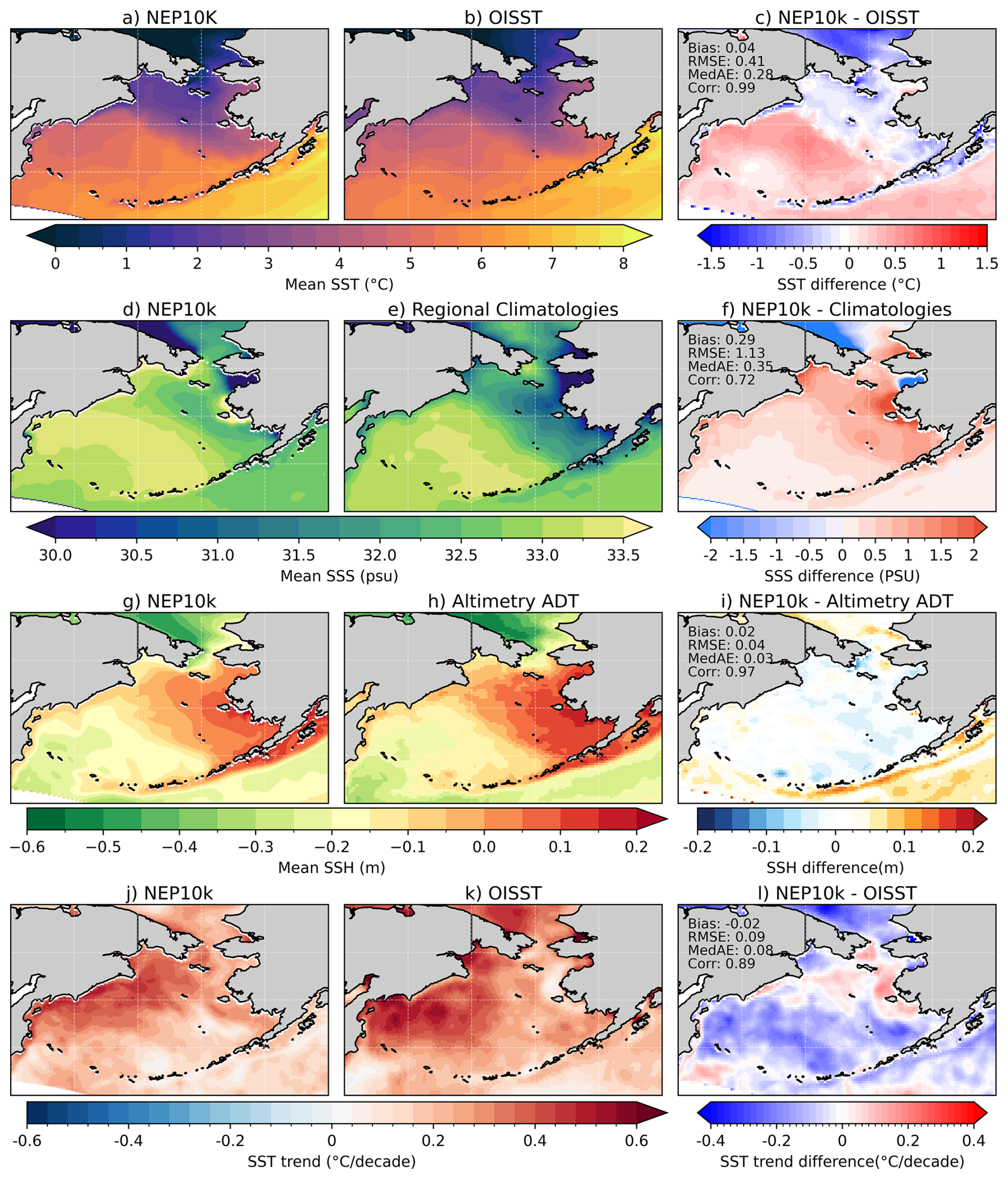
Figure 9 Mean SST (1993–2018) from (a) MOM6-NEP10K and (b) OISST, and (c) their differences. Mean SSS from (d) MOM6-NEP10K and (e) regional climatologies, and (f) their differences. Mean SSH from (g) MOM6-NEPK10K and (h) satellite altimetry, and (i) their differences. SST trends, defined by linear regression from (j) MOM6-NEP10K (k) OISST and (l) their differences. All correlation values are significant (p<0.001). Statistics of the biases (domain averaged mean bias, RMSE, Median Absolute Error (MedAE), and correlation coefficient) are indicated on panel (c), (f), (i), and (l).

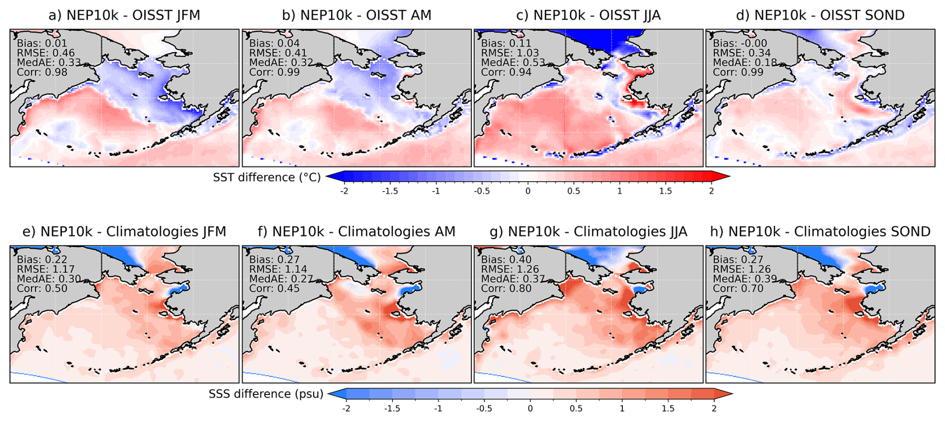
Figure 10 Difference between the 1993–2018 seasonal mean SST in the model and the OISST dataset for: (a) January–March; (b) April–May; (c) July–September; and (d) October–December. Similarly, the seasonal differences in SSS for: (e) JFM; (f) AM; (g) JAS; and (h) OND. Bias statistics are summarized in each panel.

Similar to SST, Fig. 9d–f compares mean SSS (1993–2018), simulated by model (Fig. 9d) against regional climatologies (Fig. 9e). Along the northern Siberian coast, the model is consistently fresher than the observations. This may be associated with sea-ice biases due to the closed ice boundary conditions and limited observational data. Modeled mean SSS patterns over the Bering Sea basin tend to be in good agreement with regional climatologies, with small (< 0.5 psu) discrepancies (Fig. 9f); SSS biases on the Bering Sea shelf, however, are larger than those in the basin (Fig. 9f). The saltier SSS bias on the eastern shelf coincides with colder SST biases, leading to positive sea surface density biases in the region. The positive SSS bias along the eastern Bering Sea coast tends to be stronger in JJA (Fig. 10g) than in other seasons: the model shows small positive biases during JFM and AM (Fig. 10e, f), and moderately positive bias in SOND (Fig. 10h), mainly in the central and southern inner shelf. These discrepancies may reflect underestimated freshwater input from major rivers such as the Yukon and Anadyr in the GloFAS forcing, which could affect coastal salinity and stratification patterns.

Model and observations show a similar spatial pattern in SSH (Fig. 9g–h): higher values in the central and southeastern Bering Sea shelf; decreasing SSH in the basin; and lower SSH along the north coast of Siberia in the Chukchi Sea. SSH bias over the entire Bering Sea is modest (Fig. 9i). Not unexpectedly, MOM6-NEP simulation and OISST reveal a warming trend (Fig. 9j, k). The spatial structure of SST warming is similar across the datasets, with stronger warming (> 0.3 °C/decade) along the Russian coast and in the Chukchi Sea, but weaker warming elsewhere. Nowhere is there cooling. Quantitatively, the model simulation tends to overestimate the SST warming on the northern Bering Sea shelf and in the North Pacific adjacent to the western Aleutian Islands, but underestimate it in the rest of the domain (Fig. 9l).

There is reasonable agreement between the model and observed MLD during the summer except in the southern basin (Fig. 11c). The model on average underestimates the summer MLD, although there were both positive and negative spatial patterns in the biases. MLD biases in winter increase significantly relative to summer values. The modeled winter MLDs are too deep nearly everywhere across the domain. Interestingly, the spatial correlation remains high (Fig. 11f). MLD biases can be linked to errors in surface forcing, model physics, inaccuracies in numerical algorithms, and/or uncertainties in observations, but which factor is the main contributor is unknown. MLD and its seasonal evolution affect nutrient distribution and primary production, and is crucial to the marine ecosystem dynamics of the region. Further quantifying the modeled MLD and its spatiotemporal variability, and understanding the mechanisms contributing to its biases will be a research priority in the future.

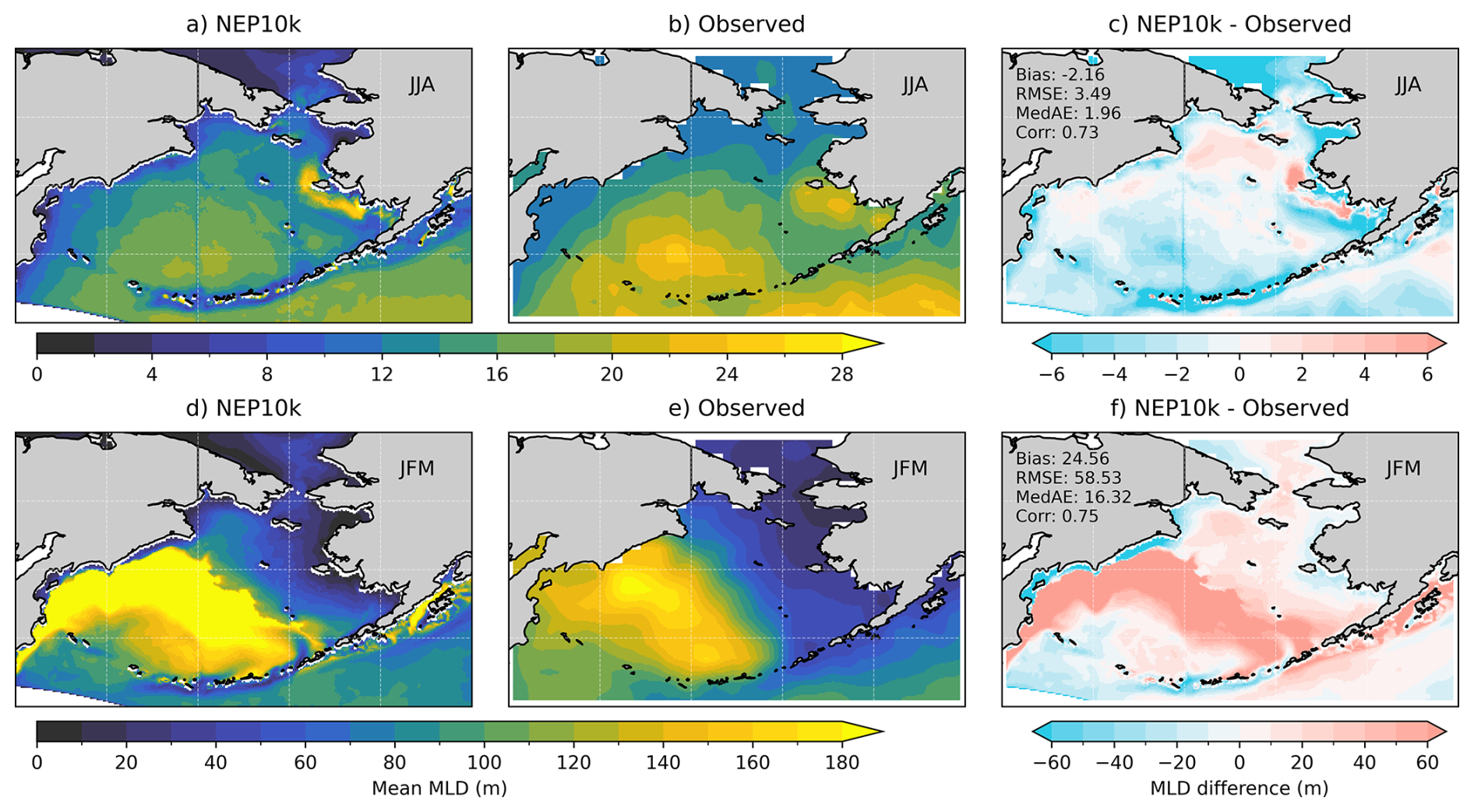
Figure 11 Mean (1993 MLD from the model for (a) summer (June–August) and (d) winter (January–February). MLD from the observation-based climatology of de Boyer Montégut (2004) for (b) summer and (e) winter. The difference between model and observations for (c) summer and (f) winter, including bias statistics.

3.5 Water column structure: temperature and salinity

3.5.1 Southeastern Bering Sea (M2)

Figure 12a illustrates the depth-time contours of temperature collected at M2. The seasonal pattern is clearly evident – warm (> 8 °C) temperatures near the surface in the summer, cooling and mixing in the fall, and cold (usually < 2 °C) temperatures throughout the water column in winter and into spring. The surface wind mixed layer in summer was ∼ 20 m deep and there is a tidally-mixed bottom layer. These seasonal patterns are accurately replicated by the model (Fig. 12b), as is the mean vertical structure during each season (Fig. S4a–d).

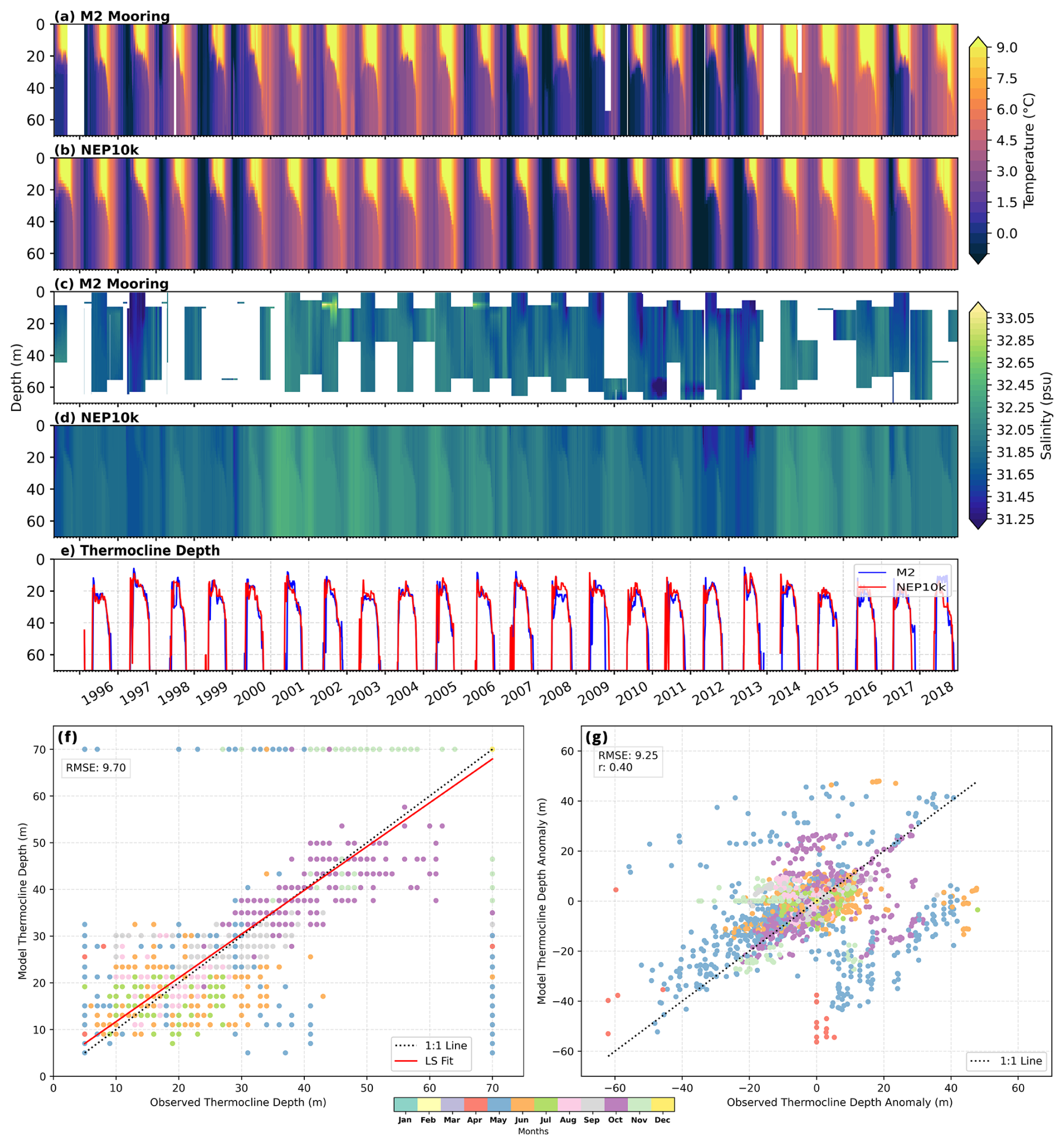
Figure 12 Depth versus time contours of temperature for (a) observations and (b) model, and salinity for (c) observations and (d) model. (e) The thermocline depth at M2 for model (red) and observations (blue). Scatter plots of: (f) observed versus modeled daily thermocline depth at M2; and (g) thermocline depth anomaly with the mean signal (1996–2018) removed.

Salinity data from the moorings are more limited, but interannual variability is evident (Fig. 12c). The water was relatively fresh in 1993–1999 and 2007–2013, and relatively salty in 2000–2005 and 2014–2018. The fresher (saltier) conditions tend to occur in colder (warmer) years, consistent with colder years having more sea ice at M2 that melts upon arrival, thus freshening the water column. This interannual variability is captured by the model (Fig. 12d), although the simulated salinity appears smoother, lacking some of the higher salinity peaks and short-term variability characteristic of the mooring data. This suggests that the model may underrepresent certain episodic salinity events, despite its ability to accurately simulate the mean salinity distribution.

The thermocline depth and strength are crucial for understanding marine ecosystems since they influence nutrient availability, primary productivity, and the distribution of marine species, thus influencing the bigger ecological and fisheries dynamics in the Bering Sea. Thus, we examine the thermocline in more detail. The observed and modeled thermocline depth (calculated using method described in Sect. 2.3) displays a clear seasonal cycle (Fig. 12e): it shoals in late spring and summer due to surface heating and reduced wind mixing, allowing the water column to stratify, and deepens in fall and winter due to surface cooling and mixing processes. The seasonal differences of mean and median are small (Fig. S3). The consistency between the observed and modeled thermocline depth suggests that the model captures the key physical process regulating seasonal stratification on the Bering Sea shelf. The relatively small discrepancies between the model and observations in certain years (e.g., 2008 in Fig. 12e) can be caused by inaccuracy in forcing functions (e.g., surface heating, winds) or subgrid scale parameterizations.

A more quantitative comparison between modeled and observed thermocline depth suggests that the water column is stratified mainly from May to October (Fig. 12f, colors of the dots) and is well mixed during the rest of the year (e.g., the points at (70, 70)). Wind-mixed deepening occurs during October (purple dots on Fig. 12f). There are generally no systematic biases between the model and observations as the data points are distributed above and below the 1:1 line.

More patterns are revealed once the annual signal is removed (Fig. 12g). Most of the data is centered around (0,0); ∼ 80 % (∼ 90 %) of the data points are within 5 m (10 m) of the origin suggesting small biases. If we just consider the summer months when the water is stratified, the percentages are less (∼ 68 % with 5 m, and ∼ 85 % within 10 m).

The greatest persistent deviations from the 1:1 line occur in May when the system usually becomes stratified (Fig. 12g, blue dots), and around October when the thermocline deepens (Fig. 12g, purple dots). These results suggest that the rapidly changing transition seasons (spring and fall) still pose challenges for modeling accuracy, which has implications for seasonal forecasting of the ocean environment and marine ecosystem across these seasons (e.g., the so-called spring predictability barrier, Duan and Wei, 2013). Overall, there are no systematic biases between the model and data.

3.5.2 Northern Bering Sea (M8)

The model simulations also reproduce the observed seasonal and interannual variability of temperature and salinity profiles at the northern mooring M8 (Fig. 13). Here temperature and salinity variability is related to sea ice, with 2018 being the warmest year throughout the water column and the year with the least ice extent (Fig. 7b). Prior to 2014, temperatures were colder both in the observations and in model simulations. The summer wind mixed layer at M8 is typically < 20 m (Stabeno et al., 2020), which is not observed since the top instrument was at ∼ 20 m to avoid ice keels. The thermocline gradient is not as sharp at M8 as at M2 (Stabeno et al., 2012a). The model replicates the penetration of heat below the mixed layer that is evident in the data. The seasonal mean vertical structure of temperature from the model are in excellent agreement with observations (Fig. S1e–h).

Figure 13 As in Fig. 12a–d for M8.

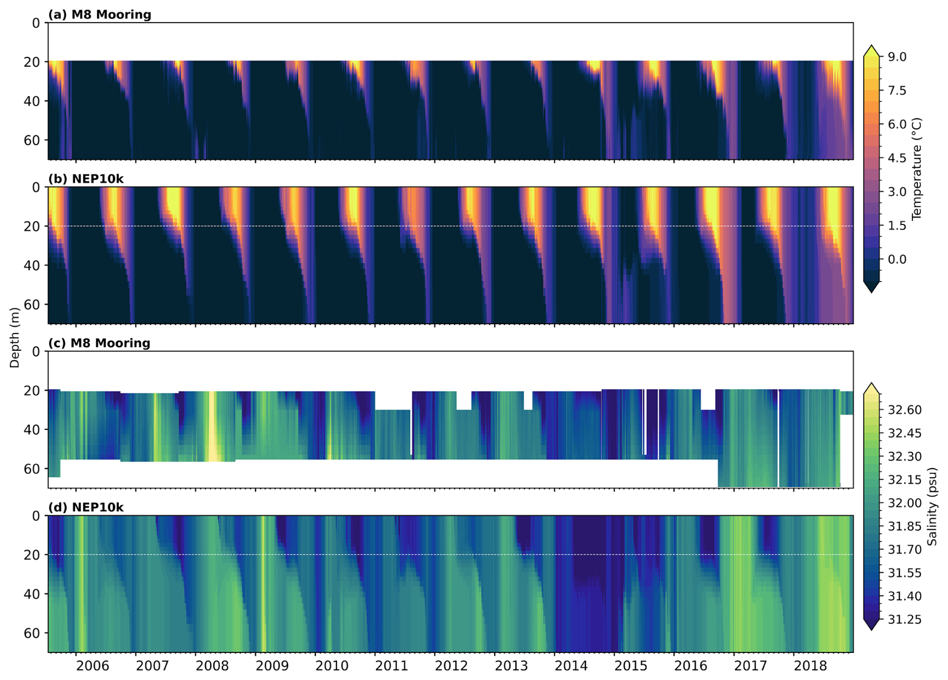
Salinity at M8 has a strong seasonal signal, with freshening occurring in the water column in fall, which is a result of mixing the fresh surface water downward; the fresh surface layer is a result of ice melt from the previous spring (note 2018 does not have this signal). Salinity is harder to measure and model than temperature. There is no natural feedback between SSS and surface freshwater fluxes, and biases of salinity in model simulations can accumulate although advection limits this bias. Despite this, the simulation captured the observed patterns of seasonal and interannual variability of water column salinity at M8, showing the penetration of fresh signal to deeper depth each autumn, and a relatively fresh period from late 2009 to 2015, and salty periods prior to 2009 and after 2016. 2014–2015 stands out as an anomalously fresh period in both OBS and model. These years had extensive ice cover at M8 in winter (Fig. 7c, d), though it is not significantly different from other years. Whether anomalies in ice thickness/volume contributed to the fresh signal in these years remains to be investigated.

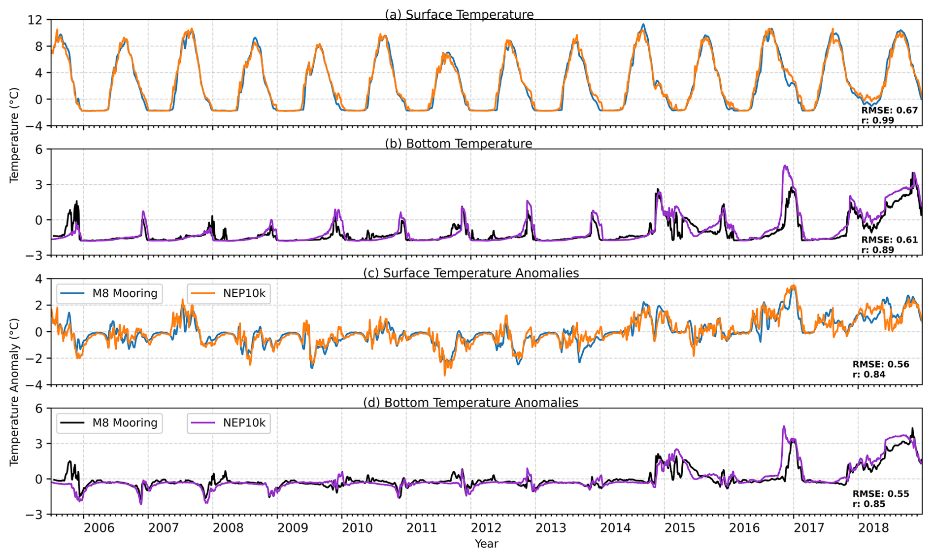
3.5.3 Surface and bottom temperatures

A more detailed statistical analysis was completed for the surface and bottom temperature at both moorings. The model replicates the annual signal both at the surface and at the bottom at M2 (Fig. 14 a, b) and at M8 (Fig. 15a, b). The interannual variability is also captured at both sites (Figs. 14c, d and 15c, d), including the warm periods (2001–2005, 2014-2018) and the cold period (2007–2013). Note that the near-surface temperature anomaly at M8 has less variability than at M2 because the top-most instrument was below the surface mixed layer during summer. At both locations, greater discrepancy between simulation and observation occurs at the near-bottom temperature after 2014, when the Bering Sea shelf shifted from cold to warmer conditions.

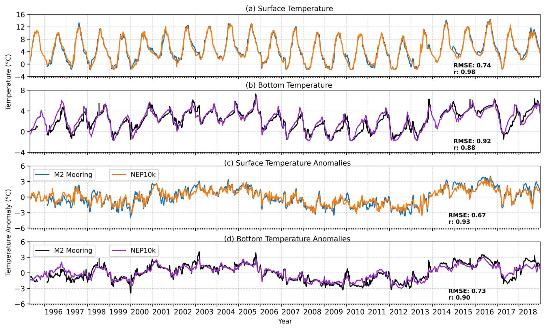
Figure 14 The time series at M2 of (a) near-surface and (b) near-bottom temperatures for model and observations (see panel c and d for line legends). Time series with the mean seasonal signal removed for: (c) near-surface temperature anomalies, and (d) near-bottom temperature anomalies. Correlation values are significant (p<0.001).

Figure 15 Same as in Fig. 14 for M8.

3.6 Bering Sea cold pool

Summer and fall ocean temperature in the eastern Bering Sea is significantly impacted by seasonal sea ice that typically forms in the fall/winter and melts in late-winter or spring (Stabeno et al., 2012b). Most of the shelf region experiences colder temperatures in years with extensive sea-ice cover that lasts late into the ice season, and warmer temperatures in years with limited sea ice cover and/or early retreat. Temperature plays a significant role in water column stratification, affecting the spatial distribution of pelagic and demersal communities (Ladd and Stabeno, 2012; Spencer et al., 2016; Grüss et al., 2021). The cold water mass that persists near the bottom as a result of sea ice melting and insulation from the surface heating during the summer is referred to as the “cold pool”. This feature limits the distribution of commercially important species such as Alaska pollock (Gadus chalcogrammus) and Pacific cod (Gadus macrocephalus). It also provides a corridor for arctic species to move southward. Historically, it was defined as waters colder than 2 °C, although other thresholds have been used. Both AFSC summer Bottom Trawl Survey and survey-replicated MOM6-NEP output show a southward extension of the cold pool along the middle shelf from the northwest to the southeast, while relatively warm temperatures occur on the inner and outer shelves during summer (Fig. 16a, b). While the long-term model and observation means of summer cold pool are similar, Fig. 16c highlights areas of discrepancy. In general, the simulation has a modest warm bias in the shallow region and a cold bias near the continental slope.

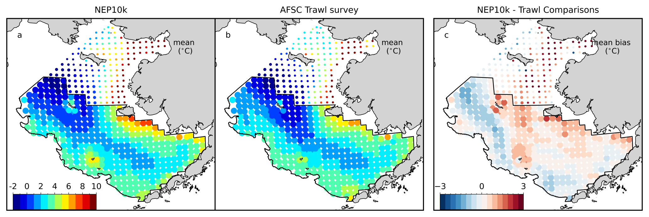
Figure 16 A comparison of Bering Sea mean (1993–2018) bottom temperatures from (a) MOM6-NEP10K (subsampled to trawl survey locations and times) and (b) AFSC trawl survey measurements. (c) The differences between the modeled (a) and AFSC trawl survey (b).

A range of cold-pool indices are defined by the proportion of the Bering Sea survey area with bottom temperatures colder than 2, 1, 0, and −1 °C. The modeled and observed interannual cold-pool indices show remarkable agreement (Fig. 17), especially for the higher (> −1 °C) temperature thresholds. Combined with the spatial patterns seen in Fig. 16, these results suggest that the model accurately represents the interannual variability and spatial extent of the cold pool. The ability of the model to replicate the cold pool dynamics is essential for understanding ecosystem dynamics and fisheries management applications.

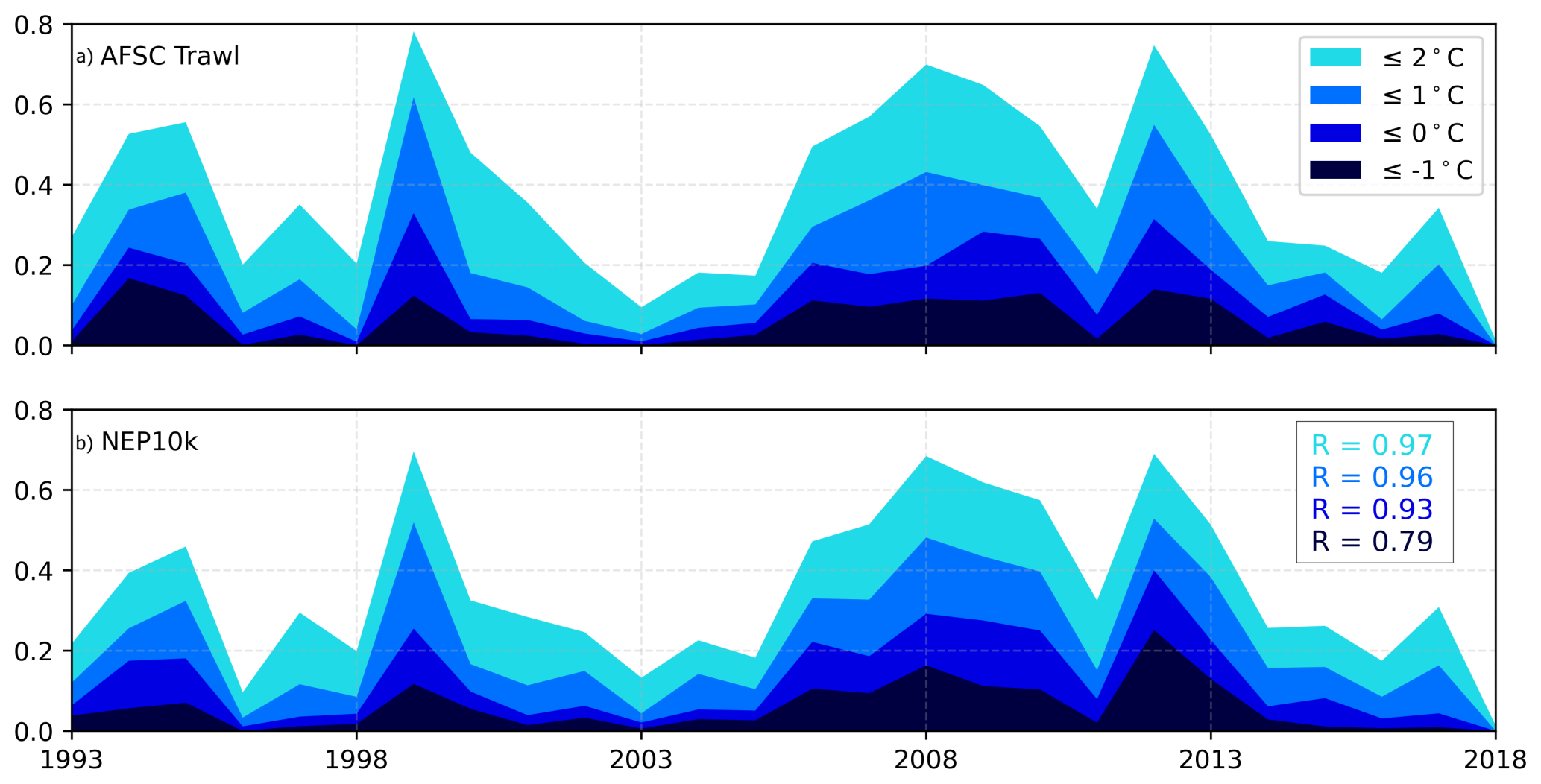
Figure 17 Cold pool indices defined as the proportion of the southeastern Bering Sea survey area (outlined by black line on Fig. 16) colder than four thresholds (2, 1, 0, and −1 °C). These summer indices are (a) AFSC trawl survey and (b) MOM6-NEP10K during 1993–2018. Correlation between the modeled and measured cold pool indices are indicated on the bottom panel.

4 Conclusions and Discussion

MOM6 has long been used in global Earth System Model simulations (Held et al., 2019). Recent improvements of MOM6 include its more advanced sub-grid scale parameterizations and the ALE vertical coordinate, which allows for larger time steps and faster integration of the model. These features make MOM6 a powerful tool for accurately and efficiently modeling ocean conditions in the past and predicting changes in the future. On the other hand, application of MOM6 in the regional modeling framework is relatively new, and only a few studies have addressed its performance in the context of high-resolution regional modeling. In this study, we evaluated a coupled ocean-sea ice model MOM6-NEP hindcast simulation (1993–2018) against satellite and in-situ observations. This study complements results in Drenkard et al. (2025), where coast-wide (from Baja to Chukchi) evaluation under a different atmospheric reanalysis forcing is presented.

We found that the model captured the main near-surface ocean circulation features on the Bering Sea basin and on the shelf. The model simulation appears to better capture weak shelf circulation features, such as flow along the 50 and 100 m isobaths, compared to previous ROMS-based efforts (Kearney et al., 2020 and references therein), where bathymetry was necessarily smoothed and flows followed the “f/H” contours too strongly, partly due to the pressure gradient errors inherent in terrain-following coordinate systems (Griffies and Treguier, 2013). Given that the shelf dynamics are sensitive to the bathymetric contours, it is critical to include realistic bathymetric features and properly render cross-isobath flows.

The original MOM6 shear-driven mixing scheme (Jackson et al., 2008) over-mixed the water column in the bottom boundary layer, especially over the energetic tidally driven southern Bering Sea shelf. This over-mixing was improved when we introduced a new scaling factor to further reduce the turbulence decay length scale near boundaries. This result points to the need for improving the interactions among surface, bottom boundary layer and interior mixing schemes. With the new scaling factor, water mass properties over the Bering Sea shelf as measured by EcoFOCI biophysical moorings are well captured by the model simulation, and in particular, the MLD and the sharp thermocline along the middle domain in summer is well preserved in the model. MLD along the Bering Sea slope still shows significant deep biases. Improvements to the model as well as observational data could bring the model and data closer together.

It is important to consider whether our rescaling of boundary effects is physically appropriate for other domains, or is unique to our region. First, note that this rescaling does not violate the ”law of the wall”, in that the vertical mixing length scale will still increase linearly with distance from the boundary, albeit at a different rate than the standard von Karman constant used in Jackson et al. (2008). Second, we note that the TKE dissipation term of Jackson et al (2008) (their Eq. 11 and its description in their text) uses buoyancy and shear length scales from local gradients, but includes no explicit influence of the nearest boundary (L_z), which could conceivably impact the TKE dissipation rate. It is possible that our rescaling of L_z indirectly compensates for unresolved boundary-related dissipation of TKE in our energetic tidal environment. Finally, we note that the Bering Sea shelf substrate includes “contemporary sediments, from 1.5 m to over 6 m thick in the southeastern region” (Smith and McConnaughey, 1999). Above this, a very thick (∼ 20 m) bottom nepheloid layer has been observed mid-shelf, and hypothesized to include tidally-resuspended sediments (Rohan et al., 2021). Such resuspension could alter the turbulent structure of the boundary layer (with consequences for the effective von Karman value), as has been observed in fluvial streams (Gaudio et al., 2010). If our rescaling primarily compensates for this local alteration, it would of course be less applicable to regions without such a nepheloid layer.

Responding to, and driving water mass properties, the modeled sea ice over the Bering Sea shelf closely matches observations in terms of shelf-wide ice extent and its mean seasonal cycle and interannual variability, as well as the long-term mean sea-ice arrival and retreat timing in both the southern and northern shelf. This is also an improvement over prior ROMS Bering Sea simulations, where modeled sea-ice concentration showed a systematic bias in its long-term mean, arriving and melting later than observations by ∼ 2 weeks (Kearney et al., 2020). Sea-ice seasonal timing is critical to the Bering Sea ecosystem dynamics. Over the northern shelf, however, ice concentration during the late-April to May melt season tends to have reduced interannual variability – the simulation has smaller (larger) ice concentration in relatively cold (warm) periods than in observations. Sea-ice over the northern shelf is highly dynamic during the melting season. The exact reasons contributing to this discrepancy remain to be understood. Another area in need of future improvement is the open boundary conditions for limited-domain sea-ice modeling. Currently, MOM6-NEP has closed ice lateral boundaries along its eastern and northern edges of the Chukchi Sea. These closed boundaries are found to degrade its performance on the Chukchi Sea shelf, where sea ice accumulated along the boundaries where in reality they are advected across the boundaries (Dukovskoy, personnel communications). The closed ice boundaries do not appear to degrade the sea-ice simulation on the Bering Sea, likely because most ice in the Bering Sea forms locally, and the missing sea-ice boundary is far to the north of the Chukchi Sea and does not affect our results.

We also investigated the Bering Sea cold pool in this study, as it plays an important role in ecosystem dynamics and is strongly influenced by seasonal sea ice. As evidenced by the agreement between AFSC trawl survey measurements and model simulations, the cold pool spatial and temporal variability is accurately replicated by the model, with a strong correlation for multiple temperature thresholds. While the model replicates the cold pool dynamics of the Bering Sea shelf where horizontal flow is weak, we also note the difference in cold pool indices between this study and Drenkard et al. (2025) (compare Fig. 17 with their Fig. 20). Note that Drenkard et al. (2025) used the same lz_rescale (β= 0.2) value as in this study. The difference in cold pool indices is likely a consequence of the difference in the two atmospheric forcing products (JRA55 in this study versus ERA5 in Drenkard et al. (2025). The uncertainties associated with different forcing data sets in regional ocean-sea ice modeling should be kept in mind when interpreting these modeling results.

In contrast to the middle shelf dynamics, there are some systematic biases between the model and trawl survey measurements near the continental slope and on the outer shelf (water depth 100–180 m) of the eastern Bering Sea. The outer shelf is a region where horizontal advection, including on-shelf flow, is often observed, especially in the deep canyons abutting the slope. The proper strength of simulated on-shelf flow in the canyons needs to be further examined.

Other near-term future work includes bringing the span of hindcast simulation closer to the present day and operationalizing its workflow. This is the first step towards building a reliable ocean modeling system capable of historical hindcasting, seasonal to interannual forecasting/prediction, and multi-decadal projections. Continued model improvements, data collection, and careful model evaluation will increase our understanding and confidence in using these modeling systems to support marine resource management decision making, which is the ultimate goal of the NOAA Changing Ecosystems and Fisheries Initiative (CEFI).