Towards the assimilation of atmospheric CO₂ concentration data in a land surface model using adjoint-free variational methods

A comprehensive understanding and accurate modelling of the terrestrial carbon cycle are of paramount importance to improve projections of the global carbon cycle and more accurately gauge its impact on global climate systems. Land surface models, which have become an important component of weather and climate applications, simulate key aspects of the terrestrial carbon cycle, such as photosynthesis and respiration. These models rely on parameterisations that require careful calibration. In this study we explore the assimilation of atmospheric CO₂ concentration data for parameter calibration of the ORganizing Carbon and Hydrology In Dynamic EcosystEms (ORCHIDEE) land surface model using an EnVarDA method, an adjoint-free ensemble-variational data assimilation method. By circumventing the challenges associated with developing and maintaining tangent linear and adjoint models, the EnVarDA method offers a very promising alternative. Using synthetic observations generated through a twin experiment, we demonstrate the ability of EnVarDA to assimilate atmospheric CO₂ concentrations for model parameter calibration. We then compare the results to a VarDA method that uses finite differences to estimate tangent linear and adjoint models, which reveals that EnVarDA is superior in terms of computational efficiency, fit to the observations, and parameter recovery.

1 Introduction

Since the link between the increase in atmospheric CO₂ concentrations and global warming was revealed, understanding the carbon cycle has become essential. This increase is mainly due to anthropogenic emissions (IPCC, 2023), half of which are absorbed by oceans and lands. To improve predictions of the carbon cycle and reduce its associated uncertainty in climate projections, it is essential to better understand the mechanisms of the carbon sink, particularly its land component, which remains the most uncertain aspect of the global carbon budget (Friedlingstein et al., 2023).

Atmospheric CO₂ concentration data have long been considered a rich source of information to understand the global carbon cycle and characterise the spatio-temporal variation in natural CO₂ fluxes (Kaminski et al., 1999a; Rayner et al., 1999; Bousquet et al., 2000; Gurney et al., 2002; Peylin et al., 2005, 2013; Chevallier et al., 2014). Given that the atmosphere is relatively well mixed, the observed concentration gradients (in space and time) can be used to identify the large-scale characteristics of the underlying surface fluxes. Indeed, surface fluxes are the primary drivers of these gradients. Studying these data gives us an overall view of all the components of the carbon cycle. For more than 25 years, atmospheric CO₂ inversions have been used to estimate natural CO₂ surface fluxes, using atmospheric transport models and Bayesian inversion frameworks (Kaminski et al., 1999b; Enting, 2002; Chevallier et al., 2005, 2007; Baker et al., 2006; Rayner et al., 2019; Berchet et al., 2021). Atmospheric transport models represent the transport of atmospheric tracers, making it possible to simulate the 3D fields of atmospheric CO₂ concentrations based on a CO₂ surface flux scenario, including all components of the carbon cycle: natural land and ocean fluxes and anthropogenic emissions from fossil fuels and cement. By inverting the atmospheric transport and using the CO₂ surface flux scenario as prior information, atmospheric inversions statistically adjust the surface CO₂ fluxes, minimising the differences between observed and modelled concentrations. This statistical optimisation generally assumes that the corrections to CO₂ surface fluxes are isotropic in time and space. This suggests that errors in surface fluxes are only correlated in space by the distance between points and not by direction. Furthermore, these errors are not strongly correlated in time. While this approach has been valuable for understanding the global carbon cycle, it only estimates net surface fluxes, with no direct information on the underlying components (i.e. photosynthesis uptake, ecosystem respiration release, fire release). Consequently, this approach is also not suitable for making future projections.

Over the same period, land surface models (LSMs) have become an important component of Earth system models, representing a wide range of interactions between the land surface and the atmosphere. As their role has expanded, these models have incorporated an increasing number of complex processes (Fisher and Koven, 2020) and have come to play a key role in weather and climate applications. LSMs now simulate key aspects of the terrestrial carbon cycle, including soil and vegetation dynamics, providing valuable insights into the main drivers of the land carbon budget and enabling future projections. Given the complexity and the small-scale nature of many of these processes, they are represented using mechanistic and empirical formulations. To accurately model these processes, LSMs rely on parameterisations that must be carefully calibrated to ensure their simulations are consistent with actual observations. One promising approach for calibrating these parameters is the use of atmospheric CO₂ concentration data, which offer a global constraint for large-scale calibration, serving as an alternative to traditional atmospheric inversions (Knorr and Heimann, 1995; Kaminski et al., 2002, 2012; Rayner et al., 2005; Scholze et al., 2007; Peylin et al., 2016; Schürmann et al., 2016; Castro-Morales et al., 2019; Bacour et al., 2023). This assimilation enables the calibration of LSM parameters by adjusting the underlying process representations rather than directly modifying the fluxes themselves. Such an approach also helps to identify structural errors within the models and enhances our understanding of the various processes involved. Once calibrated and refined, these models can be applied to generate more reliable future projections.

There is a long history of using data assimilation frameworks to calibrate LSM parameters (Rayner, 2010; MacBean et al., 2022; Raoult et al., 2024b). Most of the methods used for parameter calibration are derived from Bayesian formulations of inverse problems and are defined here as variational data assimilation (VarDA) methods. The VarDA method is inspired by the four-dimensional variational (4DVar) method, which was originally developed in the field of meteorology and Earth sciences (Talagrand and Courtier, 1987; Courtier et al., 1994; Asch et al., 2016) and has also been employed in atmospheric inversions to correct surface CO₂ fluxes (Chevallier et al., 2005; Basu et al., 2013; Liu et al., 2021). This approach is characterised by the definition of a cost function, which is typically based on a least-squares criterion. This cost function calculates two terms: (i) an observation term that computes the difference between observations and model outputs and (ii) a background term that incorporates prior knowledge of the state. The computation of both terms is performed in space and time. We define the VarDA method here, as our focus is not on directly optimising the prior state. Instead, we concentrate on time-invariant parameters used in the parameterisation that define the variable of interest, such as the net carbon flux. Therefore, while the observation term of the cost function incorporates time-distributed observations and model predictions – comparing them across multiple time points – the background term only compares prior parameter values once, as these values remain constant over time. Furthermore, with the VarDA method, a single assimilation cycle covering the entire observation period is used, which differs from the conventional 4DVar framework, which generally uses sequential cycles with shorter assimilation windows. In order to minimise this cost function, the VarDA method calculates its gradient with respect to the different parameters to be calibrated. A precise calculation of the gradient of this cost function requires the tangent linear and the adjoint models (Plessix, 2006). To obtain these models, the code must be differentiated. This task can be performed using automatic differentiation software (Giering and Kaminski, 2003), but the model code must be cleaned up, and small modifications must be made to ensure differentiation (e.g. the reformulation of minimum and maximum computations to enable a smooth transition at the edge, Schürmann et al., 2016). For some LSMs, it is possible to keep the model compliant using automatic differentiation software (Kaminski et al., 2012; Knorr et al., 2025); however, for complex community models such as ORganizing Carbon and Hydrology In Dynamic EcosystEms (ORCHIDEE) or JULES LSMs (Raoult et al., 2016), maintaining the tangent linear and adjoint models is very challenging due to their continuous evolution. In this case, one approach to calculating the gradient is to use finite differences to estimate the gradient of the cost function in order to use the VarDA method (Santaren et al., 2007; MacBean et al., 2015; Peylin et al., 2016; Bacour et al., 2019).

Several avenues of research have been explored for parameter calibration, including alternative methods to minimise the cost function and the application of new machine learning techniques (Raoult et al., 2024a, b). Ensemble methods have proven effective for the calibration of LSM parameters, such as the genetic algorithm (GA) (Santaren et al., 2014; Bastrikov et al., 2018) or Markov chain Monte Carlo (MCMC) (Ziehn et al., 2012). These methods require a large number of simulations and are primarily used with low-cost computational models and for on-site applications, as here they are relatively inexpensive. Parameter calibration in Earth system models has also been the subject of more intensive research (Hourdin et al., 2017). It has led to the development of new methods – for instance emulator-based methods (Williamson et al., 2013; Couvreux et al., 2021) – that have been used to calibrate components of Earth system models (Watson-Parris et al., 2021; Hourdin et al., 2023), such as ocean and atmospheric models (Williamson et al., 2017; Hourdin et al., 2021; King et al., 2024). In these methods, the model is replaced by an emulator – a computationally efficient statistical model designed to reproduce the behaviour of complex models – to enable numerous simulations and rule out sets of parameters that are not plausible. These methods are gaining in popularity for the calibration of LSM parameters (Dagon et al., 2020; Baker et al., 2022; McNeall et al., 2024; Raoult et al., 2024a), but they still require a large ensemble of simulations to build the emulator. More recently, an ensemble 4DVar method named 4DEnVar, implemented in Pinnington et al. (2020) for LSM parameter estimation, has proved very promising. This method uses a small ensemble to circumvent the necessity for a tangent linear and adjoint model. This 4DEnVar method has been used to estimate JULES LSM crop parameters at a single Nebraskan site (Pinnington et al., 2020) and to calibrate pedotransfer functions to improve JULES LSM soil moisture predictions over East Anglia (Pinnington et al., 2021) and the whole of the UK (Cooper et al., 2021). This method was also successfully used by Douglas et al. (2025) to calibrate the parameters of a simple carbon model in a twin experiment. Although the method was defined as a 4DEnVar in Pinnington et al. (2020) and Douglas et al. (2025), we choose to refer to it as EnVarDA to maintain consistency with the definitions previously presented.

The problem addressed in this article is the assimilation of atmospheric CO₂ data to calibrate the parameters of the ORCHIDEE LSM. For this application, we need to couple ORCHIDEE with an atmospheric transport model, which, in our case, is LMDZ, as they are historically linked and represent the land and atmospheric components of the Institut Pierre-Simon-Laplace (IPSL) Earth system model (Boucher et al., 2020). While tangent linear and adjoint models can be easily derived for the transport model (Hourdin et al., 2006; Hourdin and Talagrand, 2006), this is not the case for the ORCHIDEE LSM. Although tangent linear or adjoint models are not required for methods such as GA, MCMC, or emulator-based approaches, these methods necessitate defining a large ensemble, making them unfeasible for use in this study due to the time-consuming nature of model simulations. The purpose of this article is to present an adjoint-free data assimilation framework that facilitates the assimilation of atmospheric CO₂ concentrations. We demonstrate the potential of EnVarDA using synthetic observation data according to different criteria: (i) the differences between synthetic observations and simulations of atmospheric CO₂ concentrations, (ii) the spatial distribution of carbon fluxes and their subcomponents, and (iii) the recovery of the true parameters used to generate the synthetic observations. We also compare the performance of EnVarDA using these criteria with that of VarDA with finite differences. Section 2 presents the methods, the models, the data, and the experiments. Results are shown in Sect. 3, with discussions and conclusions in Sects. 4 and 5, respectively.

2 Method

2.1 Models and datasets

2.1.1 ORCHIDEE land surface model

ORganizing Carbon and Hydrology In Dynamic EcosystEms (ORCHIDEE; originally described in Krinner et al., 2005) is a process-based LSM that simulates the exchange of carbon, water, and energy between the surface, vegetation, and the atmosphere. It is composed of different sub-models: a fast one that calculates photosynthesis, hydrology, and energy balance every 30 min and a slow one that simulates carbon allocation in plant reservoirs, soil carbon dynamics, and litter decomposition every day. In this study, we used ORCHIDEE version 2 used in the Coupled Model Intercomparison Project Phase 6 (CMIP6) (Boucher et al., 2020; Lurton et al., 2020). This version contains significant improvements over the original version described by Krinner et al. (2005). The soil hydrology scheme is based on Richards' equation that describes vertical water fluxes for a soil depth of 2 m discretised into 11 layers (de Rosnay et al., 2002). The vertical discretisation for heat diffusion is identical to that used for water up to 2 m, extended to 90 m with a zero-flux condition at the bottom and with 18 calculation nodes in order to extrapolate the water content across the entire profile between 2 and 90 m (Wang et al., 2016). The hydrological and thermal properties of the soil are determined by soil moisture and texture. The dominant soil texture for each model grid cell is derived from the ZOBLER map (Zobler, 1999) using a classification system with three categories. The set of equations governing the soil organic matter (SOM) pools and their temporal evolution has analytical solutions driven by litter input and climate conditions, including soil temperature and humidity (Lardy et al., 2011).

The carbon fixation scheme follows the approach presented by Yin and Struik (2009) based on the FvCB model (Farquhar et al., 1980) for C₃ plants and Collatz et al. (1991) for C₄ plants. The ORCHIDEE LSM uses different types of vegetation grouped into plant functional types (PFTs) with similar structural characteristics. It distinguishes between 14 vegetation PFT classes, described in Table A1. Each grid point in the model is associated with PFT fractions prescribed using annually varying PFT maps derived from ESA's Climate Change Initiative land cover (LC) products and an LC‐to‐PFT cross‐walking approach (Poulter et al., 2015) (see https://orchidas.lsce.ipsl.fr/dev/lccci/, last access: 24 July 2025).

In this study, ORCHIDEE is run offline using 3 h ERA-Interim surface weather forcing fields (Dee et al., 2011) over 2000–2001 and aggregated to the spatial resolution of the LMDZ atmospheric transport model (2.5° latitude × 3.75° longitude). The carbon pools are brought to equilibrium following the TRENDY protocol (Sitch et al., 2024). This involves spinning up the model for 200 years, employing an analytical spin-up for soil carbon pools to bring them to equilibrium. This process uses a constant CO₂ concentration of 1700, no land-use change (LUC), and recycled ERA-Interim meteorological data from 1990 to 1999, as these are the only years where forcing data are available preceding the assimilation period. This spin-up run is followed by a transient simulation to account for the effects of disturbances, varying global atmospheric CO₂ concentration and LUC from 1800 to 1999, recycling the same meteorological data.

2.1.2 LMDZ atmospheric transport model

The atmospheric transport model used in this study is version 3 of the LMDZ general circulation model (GCM) (Hourdin and Armengaud, 1999). The LMDZ atmospheric model has been widely used to model the climate; it was implemented as the atmospheric component of the IPSL Earth system model (Dufresne et al., 2013). Its derived transport model has been used to simulate gas, particle chemistry, and greenhouse gas distributions in numerous studies (Peylin et al., 2005; Chevallier et al., 2005; Locatelli et al., 2015; Remaud et al., 2018). The advection is based on the Van Leer scheme (Van Leer, 1977), the deep convection is parameterised following the scheme of Tiedtke (1989), and turbulent mixing in the planetary boundary layer is based on a second-order local closure formalism (Hourdin and Armengaud, 1999). It uses a horizontal resolution of 2.5° (latitude) × 3.75° (longitude) and 19 sigma-pressure layers up to 3 hPa. The calculated winds (u and v) used to drive LMDZ are provided by ERA-Interim reanalysis meteorological data in order to realistically account for the temporal dependence of meteorological events. In this study, we use pre-calculated transport fields, as described in Peylin et al. (2005): they quantify the sensitivity of atmospheric concentrations at a given atmospheric station according to the space–time variability of the surface fluxes. The temporal resolution of the concentration is monthly, taking into account the daily surface fluxes of each grid cell in the model (as shown in Fig. 1). These pre-calculated transport fields have proven to be very useful – they considerably reduce computing time, given that the model only needs to be run once. They have been used to assimilate atmospheric CO₂ data in a few data assimilation studies (Peylin et al., 2016; Bacour et al., 2023). Although the version of LMDZ used in this study is outdated, the main objective of this work is to develop a framework for atmospheric data assimilation that will support future research using an updated version of LMDZ. Therefore, these pre-calculated transport fields provide a low-cost experiment to address the methodological and technical challenges that were previously presented. Nevertheless, it is important to note that the use of these pre-calculated transport fields does not allow for the evaluation of dynamic feedbacks between the surface and the atmosphere that may occur due to parameter changes. The pre-calculated transport fields were originally calculated to assimilate atmospheric CO₂ concentration data using the NOAA Earth System Laboratory's collaborative product (GLOBALVIEW-CO2, 2013). They model average monthly concentrations at 53 stations over the period of 1990–2009. The stations are located at different altitudes and in different locations on the continents and oceans around the world.

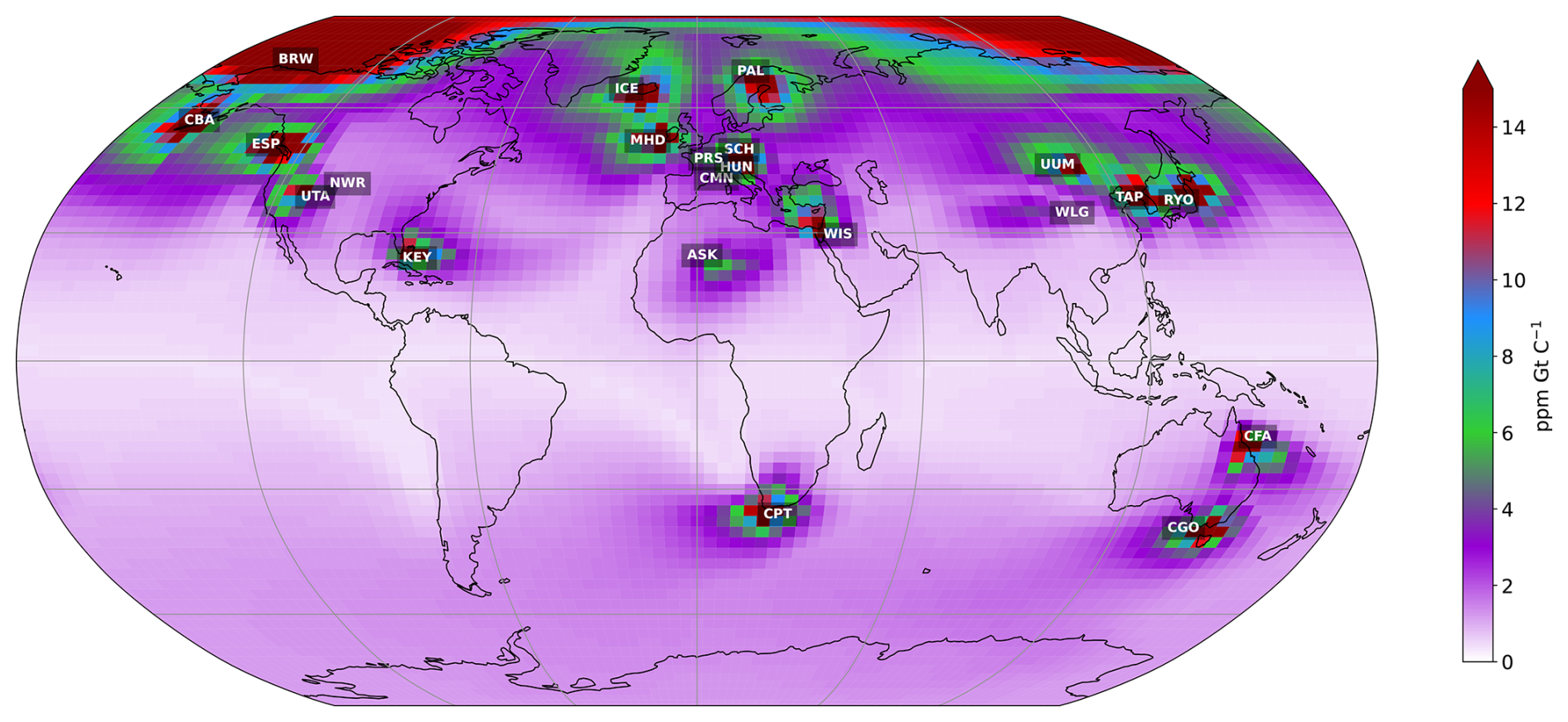
Figure 1 Monthly mean sensitivity map of atmospheric CO₂ concentrations to land carbon fluxes at the 21 stations considered over the 2000–2001 period. The average sensitivity map is obtained by deriving, for each atmospheric station and each of the 24 months, the map of the average daily sensitivity of the atmospheric concentration of CO₂ to surface carbon flux (in ppm GtC⁻¹) over the last 6 months and then calculating the average of the 24 maps. The colour of the pixel indicates the influence of the surface fluxes given by the pixel on the atmospheric concentration of CO₂, depending on the station. Red indicates a very strong influence of surface fluxes. The blue, green, and violet colours indicate different influences, from strong to weak. White indicates no influence from surface fluxes (see full details of the stations at https://gml.noaa.gov/dv/site/index.php, last access: 5 June 2025).

2.1.3 Atmospheric stations

Figure 1 shows the location of the 21 stations selected for this study. The stations were selected according to their sensitivity to continental fluxes (also shown in Fig. 1) in order to capture the temporal and spatial variations in fluxes over the continental surface. The selected stations are therefore mainly located above the land surface. The other stations, mainly located over the oceans, are less sensitive to continental fluxes, capturing mainly long-term variations. As we are only assimilating 2 years of concentrations, we choose not to take them into account. The selected stations also provide a good overview of most PFTs. However, as we can see in Fig. 1, two PFTs appear to be less sensitive to the selected stations: TrBE, which is mainly found in the tropical forests of Amazonia and Central Africa, and BoND, which is mainly found in Siberia.

2.1.4 Other components of surface CO₂ fluxes

Other components contributing to the global surface fluxes are not optimised in this study:

• The oceanic flux component was derived from a neural network model which estimated the spatial and temporal variations in CO₂ fluxes between the air and the sea (Peylin et al., 2016).

• The global maps of biomass burning emissions are taken from the Global Fire Emissions Database version 3 (Randerson et al., 2013).

• The fossil fuel CO₂ emission products used here were developed by the University of Stuttgart/IER on the basis of EDGAR v4.2.

All the fluxes used are described in greater detail in previous studies (Peylin et al., 2016; Bacour et al., 2023) and are shown in Fig. A1.

2.2 Data assimilation framework

2.2.1 A Bayesian setup

First, let us define a general Bayesian framework, mainly following Tarantola (1987, 2005), which accounts for both model/observation error and an a priori background error. Taking the approach of Kennedy and O'Hagan (2001) for an observational constraint y, let

$$\begin{array}{}\text{(1)}& \mathit{y}=\mathcal{Y}+\mathit{e},\end{array}$$

where 𝓨 represents the relevant aspect of the observed system, and e represents the error in that observation, often due to instrument error but including any error in the derivation of the data product. Let 𝓗 represent the model operator that takes the parameter vector x as input. We then assume that there exists an input x^* such that

$$\begin{array}{}\text{(2)}& \mathit{y}=\mathcal{Y}+\mathit{e}=\mathcal{H}\left({\mathit{x}}^{*}\right)+\mathit{\eta }+\mathit{e},\end{array}$$

where η represents the model error, given an imperfect model. Here, the model operator output 𝓗(x^*) and the observation y are defined in time and space. All observations are concatenated into a large vector of observations y in order to represent all observations available in a given time window. The same operation is performed for the output of operator 𝓗(x^*). Note that, given no additional information about the errors, we assume that (i) e and η are independent of 𝓨 and 𝓗(x), respectively, and (ii) both are random vector quantities following a multivariate normal distribution with a mean equal to 0 and a covariance matrix Σ_i such that $\mathit{e}\sim \mathcal{N}(\mathrm{0},{\mathbf{\Sigma }}_{\mathit{e}})$ and $\mathit{\eta }\sim \mathcal{N}(\mathrm{0},{\mathbf{\Sigma }}_{\mathit{\eta }})$. Furthermore, we assume that the parameter vector x and the model/observation likelihood y|x both follow Gaussian multivariate distributions:

$$\begin{array}{}\text{(3)}& \begin{array}{rl}& p\left(\mathit{y}\right|\mathit{x})\propto \exp \left[-{\displaystyle \frac{\mathrm{1}}{\mathrm{2}}}\left(\mathcal{H}\right(\mathit{x})-\mathit{y}{)}^T{\mathbf{R}}^{-\mathrm{1}}(\mathcal{H}\left(\mathit{x}\right)-\mathit{y})\right],\\ & p\left(\mathit{x}\right)\propto \exp \left[-{\displaystyle \frac{\mathrm{1}}{\mathrm{2}}}{\left(\mathit{x}-{\mathit{x}}_b\right)}^T{\mathbf{B}}^{-\mathrm{1}}\left(\mathit{x}-{\mathit{x}}_b\right)\right],\end{array}\end{array}$$

where x_b represents prior knowledge of the parameter vector, and B and R are the covariance error matrix for the parameter vector and for the model/observation, respectively, such that $\mathbf{R}={\mathbf{\Sigma }}_{\mathit{\eta }}+{\mathbf{\Sigma }}_{\mathit{e}}$. We seek to find the posterior distribution p(x|y) which quantifies the probability of parameters given the observations using Bayes' theorem:

$$\begin{array}{}\text{(4)}& \begin{array}{rl}p\left(\mathit{x}\right|\mathit{y})\propto & p\left(\mathit{y}\right|\mathit{x}\left)p\right(\mathit{x})\propto \exp \left[-{\displaystyle \frac{\mathrm{1}}{\mathrm{2}}}\left(\mathcal{H}\right(\mathit{x})-\mathit{y}{)}^T{\mathbf{R}}^{-\mathrm{1}}\right.\\ & \left.\left(\mathcal{H}\right(\mathit{x})-\mathit{y})-{\displaystyle \frac{\mathrm{1}}{\mathrm{2}}}(\mathit{x}-{\mathit{x}}_b{)}^T{\mathbf{B}}^{-\mathrm{1}}(\mathit{x}-{\mathit{x}}_b)\right].\end{array}\end{array}$$

2.2.2 The VarDA method

Standard VarDA

In this section, we present the VarDA method. Maximising the probability in Eq. (4) is equivalent to minimising the following function, usually referred to as the VarDA cost function:

$$\begin{array}{}\text{(5)}& \begin{array}{rl}J\left(\mathit{x}\right)& ={\displaystyle \frac{\mathrm{1}}{\mathrm{2}}}\sum _t^{N_t}\left({\mathcal{H}}_t\right(\mathit{x})-{\mathit{y}}_t{)}^T{\mathbf{R}}_t^{-\mathrm{1}}({\mathcal{H}}_t\left(\mathit{x})-{\mathit{y}}_t\right)\\ & +{\displaystyle \frac{\mathrm{1}}{\mathrm{2}}}{\left(\mathit{x}-{\mathit{x}}_b\right)}^T{\mathbf{B}}^{-\mathrm{1}}\left(\mathit{x}-{\mathit{x}}_b\right),\end{array}\end{array}$$

where t refers to time steps 0, …, N_t. Since the parameter must be constant over time, we consider only a single time window that includes all observation vectors y (in time and space). We therefore simplify the initial VarDA cost function to the compact form

$$\begin{array}{}\text{(6)}& \begin{array}{rl}J\left(\mathit{x}\right)=& {\displaystyle \frac{\mathrm{1}}{\mathrm{2}}}\left(\mathcal{H}\right(\mathit{x})-\mathit{y}{)}^T{\mathbf{R}}^{-\mathrm{1}}(\mathcal{H}\left(\mathit{x}\right)-\mathit{y})+{\displaystyle \frac{\mathrm{1}}{\mathrm{2}}}{\left(\mathit{x}-{\mathit{x}}_b\right)}^T\\ & {\mathbf{B}}^{-\mathrm{1}}\left(\mathit{x}-{\mathit{x}}_b\right),\end{array}\end{array}$$

where, for example, the concatenated vector y=(y₀, y₁, …, $y_{N_t}{)}^T$ represents all available observations at all times over the time window. The minimum of Eq. (6) can be reached iteratively using a descent algorithm that requires the computation of the gradient of J with respect to the parameter vector x. In addition, when the model is non-linear, it is common to use the quasi-Newton method to optimise the parameter vector:

$$\begin{array}{}\text{(7)}& {\mathit{x}}_{i+\mathrm{1}}={\mathit{x}}_i-{\left({\mathrm{\nabla }}^{\mathrm{2}}J\left({\mathit{x}}_i\right)\right)}^{-\mathrm{1}}\times \mathrm{\nabla }J\left({\mathit{x}}_i\right).\end{array}$$

The gradient of the cost function, ∇J(x_i), and the square matrix of partial second derivatives of the cost function (called the Hessian matrix), ∇²J(x_i), can be calculated as follows:

$$\begin{array}{}\text{(8)}& \begin{array}{rl}& \mathrm{\nabla }J\left({\mathit{x}}_i\right)={\mathbf{H}}^T{\mathbf{R}}^{-\mathrm{1}}\left(\mathbf{H}{\mathit{x}}_i-\mathit{y}\right)+{\mathbf{B}}^{-\mathrm{1}}\left({\mathit{x}}_i-{\mathit{x}}_b\right),\\ & {\mathrm{\nabla }}^{\mathrm{2}}J\left({\mathit{x}}_i\right)={\mathbf{H}}^T{\mathbf{R}}^{-\mathrm{1}}\mathbf{H}+{\mathbf{B}}^{-\mathrm{1}}.\end{array}\end{array}$$

We can update Eq. (7) using Eq. (8):

$$\begin{array}{}\text{(9)}& \begin{array}{rl}{\mathit{x}}_{i+\mathrm{1}}& ={\mathit{x}}_i-{\left[{\mathbf{H}}^T{\mathbf{R}}^{-\mathrm{1}}\mathbf{H}+{\mathbf{B}}^{-\mathrm{1}}\right]}^{-\mathrm{1}}\left[{\mathbf{H}}^T{\mathbf{R}}^{-\mathrm{1}}\left(\mathbf{H}{\mathit{x}}_i-\mathit{y}\right)\right.\\ & \left.+{\mathbf{B}}^{-\mathrm{1}}\left({\mathit{x}}_i-{\mathit{x}}_b\right)\right].\end{array}\end{array}$$

Here, the notation 𝓗 becomes H because it does not represent the use of the direct operator 𝓗. Instead, we use the tangent linear model H and the adjoint model H^T. Usually, these two terms are coded directly, but for complex models, it is usually very difficult to code and maintain these terms, especially when the model is subject to many developments (which means that they quickly become obsolete).

Epsilon-based VarDA variant: ϵ-VarDA

To approximate the tangent linear and adjoint models, we can use finite differences:

$$\begin{array}{}\text{(10)}& \mathbf{H}={\displaystyle \frac{\mathcal{H}(\mathit{x}+\mathrm{\Delta }\mathit{x})-\mathcal{H}\left(\mathit{x}\right)}{\mathrm{\Delta }\mathit{x}}},\end{array}$$

where Δx represents a small change in x. This estimate will not be as accurate as the exact tangent linear and adjoint models, but it can still help us in our minimisation objective. The accuracy of the tangent linear and adjoint models is then completely dependent on the choice of Δx. A selection of Δx that is too small may lead to H being insensitive to the parameter vector; i.e. $\mathcal{H}(\mathit{x}+\mathrm{\Delta }\mathit{x})-\mathcal{H}\left(\mathit{x}\right)=\mathbf{H}\mathrm{\Delta }\mathit{x}\approx \mathbf{0}$. This leads to the term corresponding to the difference between the observation and the output's operator (Hx_i−y) becoming negligible in Eq. (8) and hence resulting in an ineffective minimisation. By contrast, if the choice of Δx is too large, the result gives inaccurate tangent linear and adjoint models that lose their local vision around x. This results in a large loss of information and therefore a much less accurate minimisation. In our case, we define ϵ such that $\mathrm{\Delta }\mathit{x}={\mathit{x}}_{\mathrm{range}}\times \mathit{ϵ}$, where ${\mathit{x}}_{\mathrm{range}}={\mathit{x}}_{\max }-{\mathit{x}}_{\min }$, and we refer to this method as ϵ-VarDA. Due to this approximation, ϵ-VarDA is therefore not entirely equivalent to standard VarDA.

2.2.3 The EnVarDA method

From VarDA to EnVarDA

We present here an implementation of VarDA that we do not use in this study but that is important for understanding the EnVarDA method. This implementation is presented in several studies (Courtier et al., 1994; Gilbert and Lemaréchal, 1989; Liu et al., 2008; Bannister, 2016; Pinnington et al., 2020) and can be applied when the prior error covariance matrix B becomes large and difficult to invert. It is possible to introduce a matrix U and a vector w to ensure that the VarDA cost function converges as efficiently as possible and avoids the explicit calculation of the matrix B given by

$$\begin{array}{}\text{(11)}& \mathbf{B}={\mathbf{UU}}^T\end{array}$$

and

$$\begin{array}{}\text{(12)}& {\mathit{x}}_a={\mathit{x}}_b+\mathbf{U}\mathit{w},\end{array}$$

where x_a represents the posterior value of the parameter vector. Consequently, this changes the J cost function, which is presented in detail in Courtier et al. (1994):

$$\begin{array}{}\text{(13)}& \begin{array}{rl}J\left(\mathit{w}\right)& ={\displaystyle \frac{\mathrm{1}}{\mathrm{2}}}(\mathbf{HUw}+\mathcal{H}\left({\mathit{x}}_b\right)-\mathit{y}{)}^T{\mathbf{R}}^{-\mathrm{1}}\left(\mathbf{HUw}\right.\\ & \left.+\mathcal{H}\left({\mathit{x}}_b\right)-\mathit{y}\right)+{\displaystyle \frac{\mathrm{1}}{\mathrm{2}}}{\mathit{w}}^T\mathit{w},\end{array}\end{array}$$

and its gradient:

$$\begin{array}{}\text{(14)}& \mathrm{\nabla }J\left(\mathit{w}\right)={\mathbf{U}}^T{\mathbf{H}}^T{\mathbf{R}}^{-\mathrm{1}}\left(\mathbf{HUw}+\mathcal{H}\left({\mathit{x}}_b\right)-\mathit{y}\right)+\mathit{w}.\end{array}$$

EnVarDA

The EnVarDA method described in Liu et al. (2008) and Pinnington et al. (2020) incorporates an aspect of the ensemble Kalman filter (EnKF) in order to avoid the calculation of tangent linear or adjoint models necessary for VarDA. The EnKF is a Kalman filter but uses a set of N parameter vectors, also known as ensemble members, to estimate the prior error covariance matrix B (Evensen, 1994). The perturbation matrix is defined as:

$$\begin{array}{}\text{(15)}& {\mathbf{X}}_b^{\prime }={\displaystyle \frac{\mathrm{1}}{\sqrt{N-\mathrm{1}}}}\left({\mathit{x}}_{\mathrm{1}}-{\mathit{x}}_b;{\mathit{x}}_{\mathrm{2}}-{\mathit{x}}_b;\mathrm{\dots };{\mathit{x}}_N-{\mathit{x}}_b\right),\end{array}$$

where the ensemble members x_i for i=1, …, N are generated according to a multivariate normal distribution using x_b as the mean and B as the covariance matrix: 𝒩(x_b,B). It follows that

$$\begin{array}{}\text{(16)}& \mathbf{B}\approx {\mathbf{X}}_B^{\prime }\mathbf{X}{{}^{\prime }}_B^T.\end{array}$$

Using the same logic as Eq. (12), we can use the perturbation matrix as follows:

$$\begin{array}{}\text{(17)}& {\mathit{x}}_a={\mathit{x}}_b+{\mathbf{X}}_b^{\prime }\mathit{w},\end{array}$$

where w is a vector of length N. The cost function in Eq. (13) is updated accordingly:

$$\begin{array}{}\text{(18)}& \begin{array}{rl}J\left(\mathit{w}\right)& ={\displaystyle \frac{\mathrm{1}}{\mathrm{2}}}{\left({\mathbf{HX}}_b^{\prime }\mathit{w}+\mathcal{H}\left({\mathit{x}}_b\right)-\mathit{y}\right)}^T{\mathbf{R}}^{-\mathrm{1}}\left({\mathbf{HX}}_b^{\prime }\mathit{w}\right.\\ & \left.+\mathcal{H}\left({\mathit{x}}_b\right)-\mathit{y}\right)+{\displaystyle \frac{\mathrm{1}}{\mathrm{2}}}{\mathit{w}}^T\mathit{w},\end{array}\end{array}$$

and the gradient in Eq. (14) becomes

$$\begin{array}{}\text{(19)}& \mathrm{\nabla }J\left(\mathit{w}\right)=\mathbf{X}{{}^{\prime }}_b^T{\mathbf{H}}^T{\mathbf{R}}^{-\mathrm{1}}\left({\mathbf{HX}}_b^{\prime }\mathit{w}+\mathcal{H}\left({\mathit{x}}_b\right)-\mathit{y}\right)+\mathit{w}.\end{array}$$

Note that the minimisation problem changes. In both cases, we try to balance the cost function between the background term and the observation term, but we no longer aim to find x such that 𝓗(x)≈y; rather, we now look for w that determines the linear combination ${\mathbf{HX}}_b^{\prime }\mathit{w}$ which is equal to the distance δy such that $\mathit{\delta }\mathit{y}\approx \mathcal{H}\left({\mathit{x}}_{\mathrm{b}}\right)-\mathit{y}$. The ${\mathbf{HX}}_b^{\prime }$ term can be approximated by applying the 𝓗 operator to each parameter vector x present in ${\mathbf{X}}_b^{\prime }$:

$$\begin{array}{}\text{(20)}& \begin{array}{rl}{\mathbf{HX}}_b^{\prime }\approx & {\displaystyle \frac{\mathrm{1}}{\sqrt{N-\mathrm{1}}}}\left(\mathcal{H}\left({\mathit{x}}_{\mathrm{1}}\right)-\mathcal{H}\left({\mathit{x}}_b\right);\mathcal{H}\left({\mathit{x}}_{\mathrm{2}}\right)-\mathcal{H}\left({\mathit{x}}_b\right)\right.,\\ & \left.\mathrm{\dots },\mathcal{H}\left({\mathit{x}}_N\right)-\mathcal{H}\left({\mathit{x}}_b\right)\right).\end{array}\end{array}$$

where each 𝓗(x_i) is a concatenated vector of extracted simulations to correspond with all observations available at all times across the time window. Each coefficient w_i of w multiplies a vector 𝓗(x_i)−𝓗(x_b) present in the approximation of ${\mathbf{HX}}_b^{\prime }$, which represents the distance between a member of the ensemble and the prior information. The optimisation of w is performed so that the linear combination ${\mathbf{HX}}_b^{\prime }\mathit{w}$ converges around δy and taking into account the background terms. Once optimised, the vector w can be used for another linear combination ${\mathbf{X}}_{\mathbf{b}}^{\prime }\mathit{w}$, this time in the input space. This gives x_a, the posterior value of the parameter vector, which can be obtained using Eq. (17). The great advantage of this method lies in the way the gradient is computed, in particular, the term $\mathbf{X}{{}^{\prime }}_b^T{\mathbf{H}}^T$, which is equivalent to $(\mathbf{HX}{{}^{\prime }}_b{)}^T$. This equivalence makes it possible to rewrite the gradient by “simply” transposing the matrix ${\mathbf{HX}}_b^{\prime }$:

$$\begin{array}{}\text{(21)}& \mathrm{\nabla }J\left(\mathit{w}\right)={\left({\mathbf{HX}}_b^{\prime }\right)}^T{\mathbf{R}}^{-\mathrm{1}}\left({\mathbf{HX}}_b^{\prime }\mathit{w}+\mathcal{H}\left({\mathit{x}}_b\right)-\mathit{y}\right)+\mathit{w}.\end{array}$$

Subsequently, tangent linear and adjoint models are no longer required. The subjective choice here is no longer related to the choice of ϵ that estimates the tangent linear and adjoint models but to the number N of ensemble members used to generate ${\mathbf{X}}_b^{\prime }$ and ${\mathbf{HX}}_b^{\prime }$. A posterior ensemble can be obtained as described by Douglas et al. (2025) by calculating ${\mathbf{X}}_a^{\prime }$, where

$$\begin{array}{}\text{(22)}& {\mathbf{X}}_a^{\prime }={\mathbf{X}}_b^{\prime }{\left(\mathbf{I}+{\left({\mathbf{HX}}_b^{\prime }\right)}^T{\mathbf{R}}^{-\mathrm{1}}{\mathbf{HX}}_b^{\prime }\right)}^{-\frac{\mathrm{1}}{\mathrm{2}}}.\end{array}$$

2.2.4 Implementation into ORCHIDAS

The ORCHIDEE data assimilation system (ORCHIDAS) is a system designed to calibrate the parameters of ORCHIDEE and is developed in Python. It has been used for over 15 years (MacBean et al., 2022), mainly for studies focusing on the carbon cycle and other terrestrial cycles such as the water and energy budget, methane, and nitrogen (see the full list of studies published at https://orchidas.lsce.ipsl.fr/publications.php, last access: 24 July 2025).

This system has long used VarDA as described in Sect. 2.2.2, but it also allows for the use of several methods, such as genetic algorithms (Bastrikov et al., 2018) or history matching (Raoult et al., 2024a). ORCHIDAS facilitates the testing of various data assimilation methods while maintaining a consistent configuration for ORCHIDEE execution. In this study, we implemented the EnVarDA method as described in the EnVarDA section.

2.3 Experiment design

2.3.1 Twin experiment description

To test the data assimilation methods presented in Sect. 2.2, we conducted a so-called twin experiment to evaluate their efficiency in calibrating parameters involved in calculating net biome productivity (NBP) fluxes in the ORCHIDEE LSM. This experimental framework reduces the complexities associated with model–data errors, focusing on the performance of the assimilation methods. The known “true” parameters, which are the default parameter values of the ORCHIDEE model, are used to generate the synthetic observations. New values of a priori parameters are manually generated, ensuring physically meaningful values that differ from the true parameters, both of which are presented in Table A2. The assimilation methods are then applied to assess how closely they converge toward the known solution (standard parameter values). The synthetic observations of atmospheric CO₂ concentrations from the 21 continental stations are assimilated simultaneously over a 2-year window (2000–2001) to monitor spatial and temporal variations in carbon fluxes, as shown in Fig. A4. A limited period was chosen for practical reasons to avoid computationally expensive simulations.

2.3.2 Generation of synthetic observations

To generate synthetic observations for the twin experiment, we simulate net biome productivity (NBP) fluxes at the global scale using the ORCHIDEE LSM with default parameter values, referred to as the true parameters (see Table A2). These NBP fluxes represent the net carbon fluxes of the land component, calculated as the difference between emission fluxes (heterotrophic and autotrophic respiration and disturbance fluxes due to land-use change) and sink fluxes (primarily due to photosynthesis). The concentrations given by the surface fluxes (the simulated NBP fluxes, along with other fluxes described in Sect. 2.1.4) are transported using pre-calculated transport fields of the LMDZ model over the 2000–2001 period. We then extract atmospheric CO₂ concentrations at 21 continental atmospheric stations, shown in Fig. 1, which are highly sensitive to continental carbon fluxes, providing significant constraints on the parameters. This process enabled the generation of synthetic observations of monthly average atmospheric CO₂ concentrations at these 21 stations over the 2-year period. It is important to note that the steps taken here to generate the synthetic observations are exactly the same as those used to perform the simulation. This means that there is at least one solution where the model can perfectly match the synthetic observation.

2.3.3 Simplified case

First, we focus on a simplified case involving the calibration of only one PFT-dependent parameter: Vcmax, which controls the maximum rate of carboxylation limited by RuBisCO activity at 25 °C. This parameter was chosen because its impact on the atmospheric CO₂ concentration is well understood – when its value increases, the quantity of carbon absorbed by photosynthesis increases and atmospheric concentrations decrease and vice versa. The aim of the assimilation is to recover the true values of Vcmax for the 14 PFTs, resulting in the calibration of 14 parameters. This simplified case is very useful for performing several tests, allowing for a better understanding of the behaviour of the different data assimilation methods.

2.3.4 Complex case

To assess the performance of the different approaches in conditions resembling real cases, we perform another twin experiment in which we calibrate four PFT-dependent parameters and one global parameter involved in different bio-geophysical processes. The parameters selected have already been optimised in previous data assimilation studies using atmospheric CO₂ concentrations (Peylin et al., 2016; Bacour et al., 2023). In addition to Vcmax, we choose the following:

• the PFT-dependent parameter specific leaf area (SLA), which impacts leaf biomass and hence ecosystem photosynthetic capacity;

• the global parameter Q₁₀, which controls the thermal dependence of heterotrophic respiration;

• the PFT-dependent parameter m_maint.resp, which defines the slope of the maintenance respiration coefficient that controls autotrophic respiration;

• the PFT-dependent parameter LAI_max, which controls the maximum leaf area index for carbon allocation (once the LAI reaches LAI_max, no carbon is allocated to the leaf, which impacts the vegetation biomass and therefore acts on both photosynthesis and respiration).

A total of 57 ($\mathrm{14}\times \mathrm{4}+\mathrm{1}$) parameters are calibrated. As they interact within the same modelled processes, the degree of equifinality is significant.

2.3.5 Error covariance matrices

To implement the two data assimilation methods, ϵ-VarDA and EnVarDA, we define two error covariance matrices: R and B. These matrices are configured to be diagonal, as we assimilate synthetic observations, and are common to both methods to ensure comparable experiments. Their configurations are informed by previous data assimilation studies using ORCHIDEE and a simplified carbon model (Kuppel et al., 2012, 2013; Bastrikov et al., 2018; MacBean et al., 2016), with Peylin et al. (2016) specifically applying diagonal matrices for atmospheric CO₂ observations.

R matrix

The R matrix represents the model structural and observation errors. In our twin experiment setup, we choose to add only very small errors in the synthetic observations to compare both methods in an ideal case. In this context, structural errors in the ORCHIDEE LSM (i.e. missing processes) and in the transport model (i.e. coarse spatial resolution and wind biases) and measurement errors are discarded. Indeed, since the synthetic observations are generated by a simulation, as detailed in Sect. 2.3.2, there exists at least one solution where all observations can be matched perfectly. For this reason, we use a simplified R matrix with the same small diagonal terms of 0.01 ppm for all stations. The rationale behind this choice is that, as all stations can be matched perfectly, we do not want to introduce any spatial or temporal preferences.

B matrix

The B matrix represents the background errors associated with prior knowledge of the parameters. We set the error to 30 % of the parameter range for the simple case and 20 % for the complex case (as we use larger parameter ranges for this case). The background errors of each parameter can be seen in Fig. 3 for the simple case and in Fig. 6 and Table A2 for the complex case.

2.3.6 Tuning ϵ for gradient calculation

As explained in Sect. 2.2.2, the choice of ϵ is essential for effective ϵ-VarDA performance. One way to select an appropriate ϵ is to perform an ϵ test which calculates the partial derivative of 𝓗 for each of the parameters using different ϵ. We calculate the partial derivative as follows:

$$\begin{array}{}\text{(23)}& {\displaystyle \frac{\partial \mathcal{H}}{\partial \mathit{x}}}={\displaystyle \frac{\mathcal{H}(\mathit{x}+\mathrm{\Delta }\mathit{x})-\mathcal{H}\left(\mathit{x}\right)}{\mathrm{\Delta }\mathit{x}}},\end{array}$$

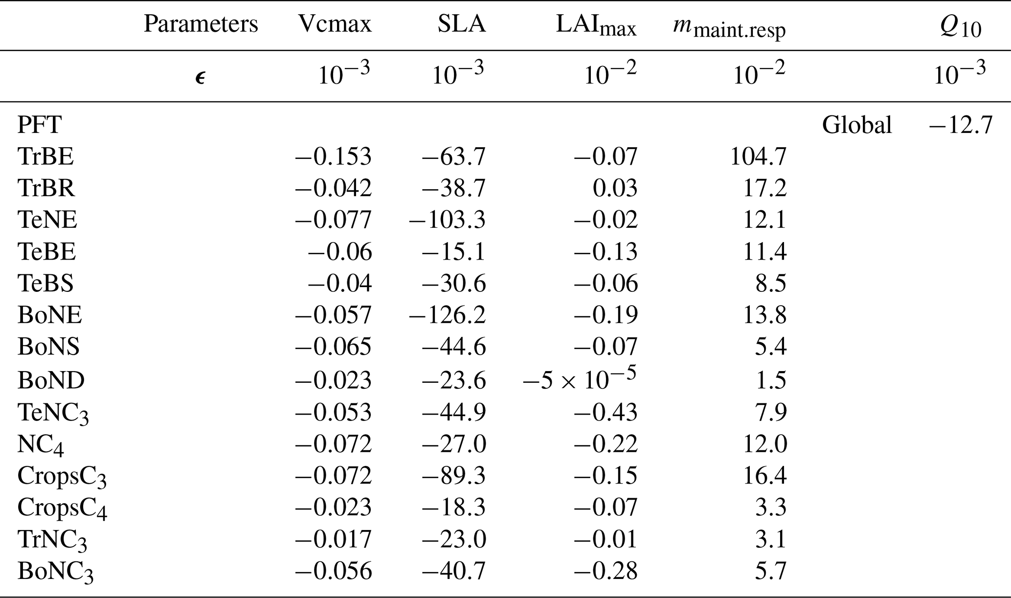
where ϵ defines Δx as explained in Sect. 2.2.2. By changing ϵ we change Δx, and we can attempt to find the value of ϵ for which the derivative becomes stable. Figure 2 shows the sensitivity of ϵ, ranging from 10⁻⁸ to 10⁻², on the calculated partial derivative of each Vcmax. We see that the partial derivative of Vcmax is unstable with an ϵ below 10⁻³ for all PFTs. Therefore, we need a value of ϵ greater than 10⁻³ to ensure correct gradient calculation with respect to the Vcmax parameter. Table A3 shows the values of the mean of the partial derivatives for all parameters and PFTs using an ϵ that allows for a stable derivative. This also allows us to check the consistency of the derivation calculation. For example, the increase in Vcmax leads to an increase in the photosynthetic capacity and subsequently in the carbon uptake by vegetation. This leads to a reduction in atmospheric CO₂ concentrations. We can see in Table A3 that the values obtained for Vcmax are negative, which is the expected response. The same ϵ test was carried out for the other four parameters used in the complex case, and the results are shown in Fig. A2 and Table A3:

• The partial derivative of SLA diverges with an ϵ below 10⁻³ for all PFTs. SLA has the same impact that Vcmax has on atmospheric CO₂ concentrations, so the negative mean values obtained are expected.

• The partial derivative of Q₁₀ does not diverge for any values of ϵ. As expected, the mean value of its derivation is negative. Increasing Q₁₀ increases the thermal dependence of heterotrophic respiration and consequently reduces it; with less heterotrophic respiration the atmospheric CO₂ concentration decreases.

• The partial derivative of m_maint.resp diverges with different ϵ values depending on the PFT, ranging from 10⁻⁵ for PFT TrBE to 10⁻² for PFT CropsC₄. This may be due to different distributions and proportions of PFTs (see Table A1). However, the mean values at 10⁻² are all positive. m_maint.resp has an impact on autotrophic respiration; increasing this parameter increases vegetation respiration and therefore the atmospheric CO₂ concentration.

• The partial derivative of LAI_max diverges with an ϵ below 10⁻² for all PFTs. Determining the sign of the mean values of the partial derivative of this parameter is not trivial here. LAI_max influences vegetation biomass and therefore photosynthesis and respiration. All PFTs give negative mean values for their partial derivative; only the PFT TrBR gives a positive mean value.

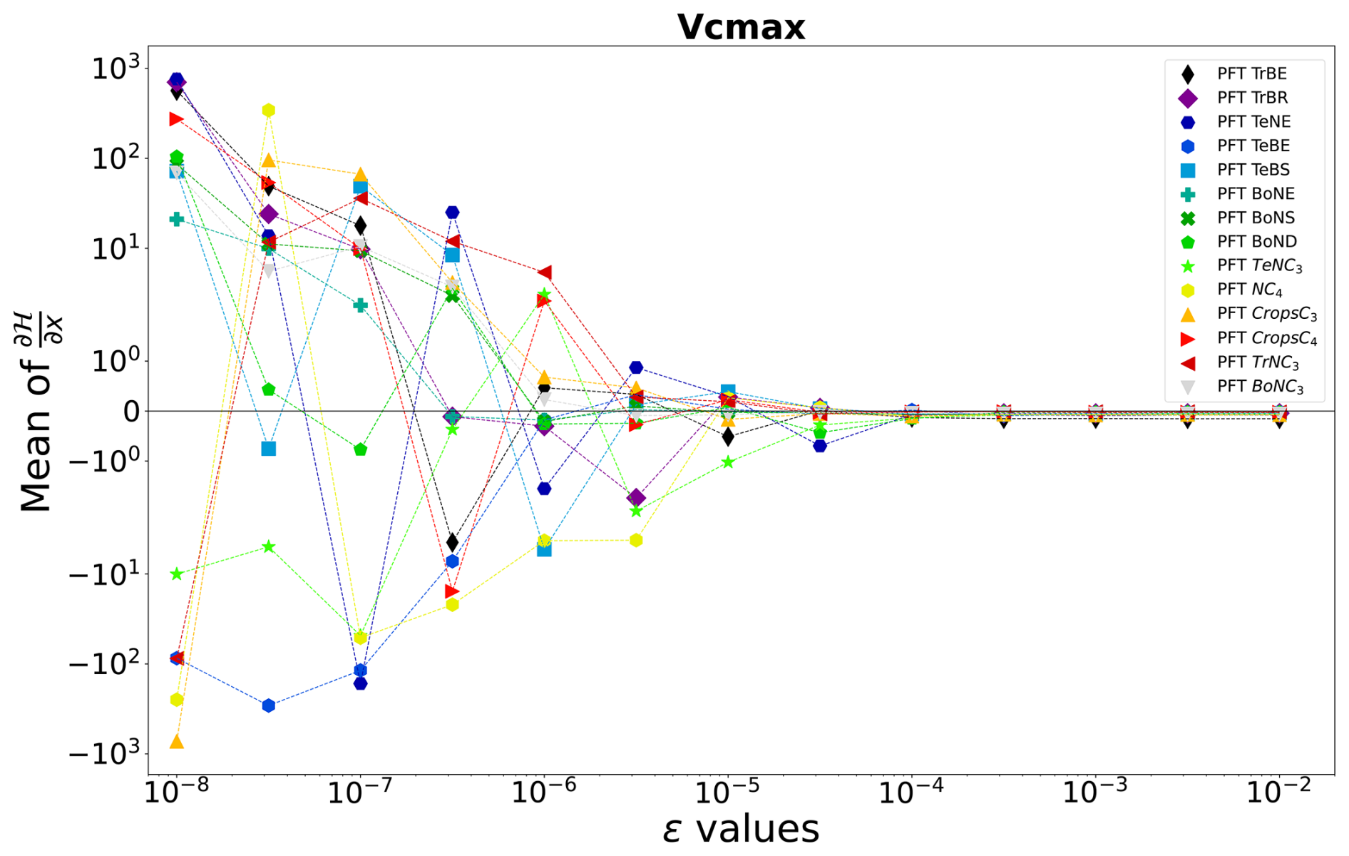
Figure 2 ϵ test: spatial and temporal average of the partial derivative of 𝓗 as a function of ϵ. The partial derivative of 𝓗 is calculated with respect to the parameter Vcmax for each PFT. It is calculated on the concentration space using every station over 2 years. The mean of the partial derivative is then calculated over space and time in order to visualise the local derivative. The derivative of 𝓗 is calculated for several ϵ.

2.3.7 Defining the impact of the configuration

For both methods, ϵ-VarDA and EnVarDA, the configuration used plays an important role in the quality of the minimisation of the associated cost function and thus the calibration of the parameter. Whether it is the choice of ϵ in ϵ-VarDA or the number of members used to generate the ensemble in EnVarDA, it is up to the user to make a choice, which can only be subjective. To assess the impact of these choices, we launch the twin experiment using different configurations:

• For the simple case, we use five different values of ϵ for ϵ-VarDA based on the sensitivity test presented in Sect. 2.3.6 and five different ensemble sizes in EnVarDA.

• For the complex case, we use five different ensemble sizes in EnVarDA and one different value of ϵ in ϵ-VarDA.

For the complex case using ϵ-VarDA, ϵ is selected relative to the results in the simple case and Fig. A2. Re-tuning ϵ for each parameter requires too many simulations and is therefore not feasible for the complex case.

For each minimisation, the limited memory Broyden–Fletcher–Goldfarb–Shanno algorithm with bound constraints (L-BFGS-B) is used (Byrd et al., 1995). For ϵ-VarDA, we set the maximum number of iterations at 40 due to computing costs. Indeed, each iteration requires N_param+1 model simulations. In each case, a solution is reached after 20 iterations (subsequent iterations are only minor corrections to the solution obtained). For EnVarDA, no maximum iteration limit is chosen, since an iteration does not require further simulation of the model (all required information is contained in the pre-calculated ensemble). We can therefore wait for the L-BFGS-B minimiser to converge, i.e. until the gradient becomes null.

3 Results

3.1 Comparing the different configurations

The results in terms of (1) the mean reduction in the root mean square difference (RMSD) calculated between the pseudo-observation and the simulation over the 2 years of the assimilation window for the 21 atmospheric stations, (2) the mean absolute differences (MAD) in parameter space, and (3) the computational demand of each experiment using the simple case are summarised in Table 1. We see that for the ϵ-VarDA method, the best results are obtained with an ϵ equal to $\mathrm{5}\times {\mathrm{10}}^{-\mathrm{2}}$, where the mean RMSD reduction is 82.3 % and the MAD score is 1.7. The best results for the EnVarDA method are obtained using an ensemble of 100 members, where the mean RMSD reduction is 97 % and the MAD score is 0.3. These two configurations are therefore considered for the simple case of the twin experiment in Sect. 3.2.1.

Table 1 Mean RMSD reduction score between the synthetic observations and posterior simulations of the atmospheric CO₂ concentration at 21 atmospheric stations, the mean absolute difference (MAD) score computed between the true parameter values used to generate the synthetic observations and the posterior parameters, and the number of simulations used for each configuration of ϵ-VarDA and EnVarDA for the simple case.

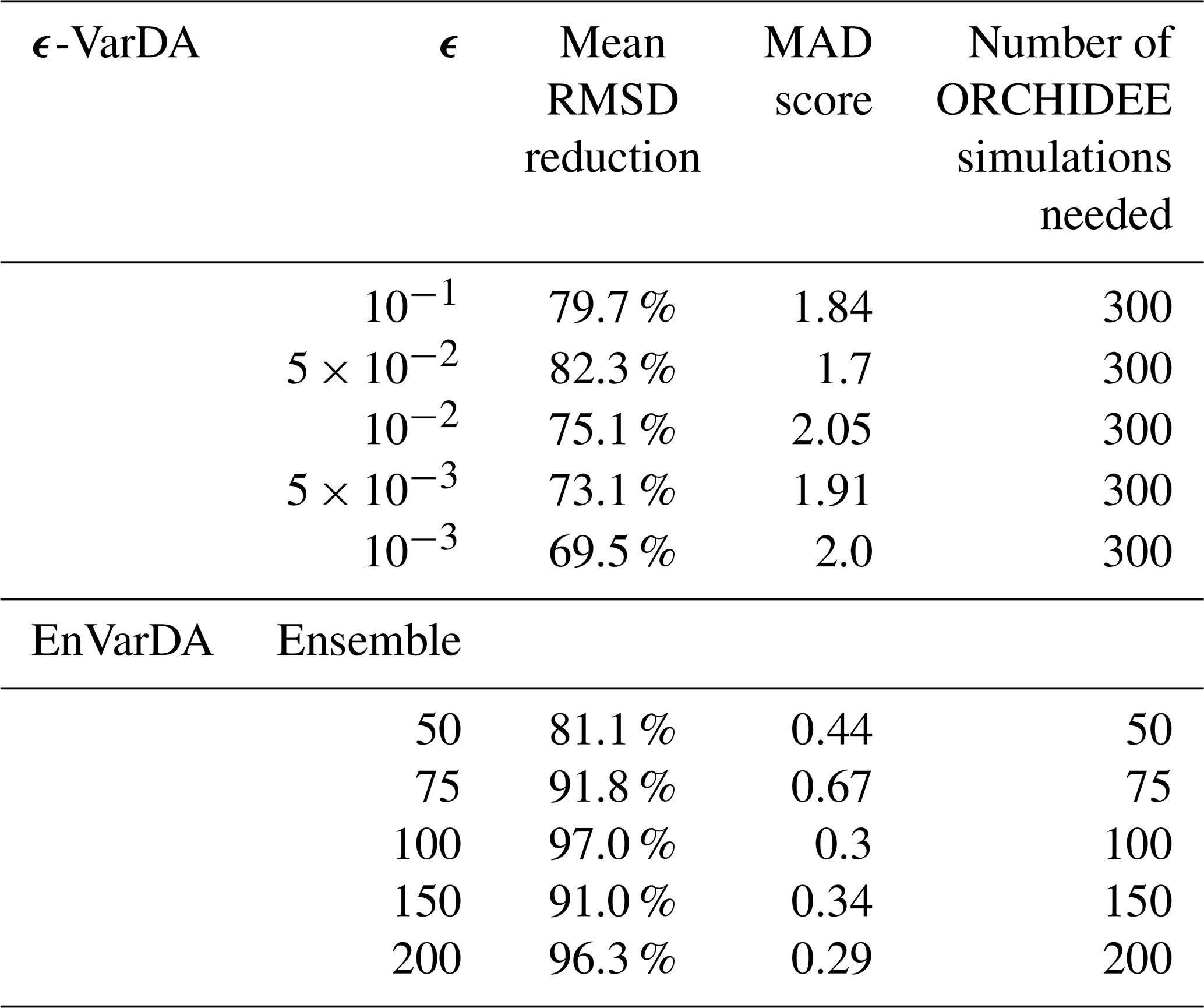
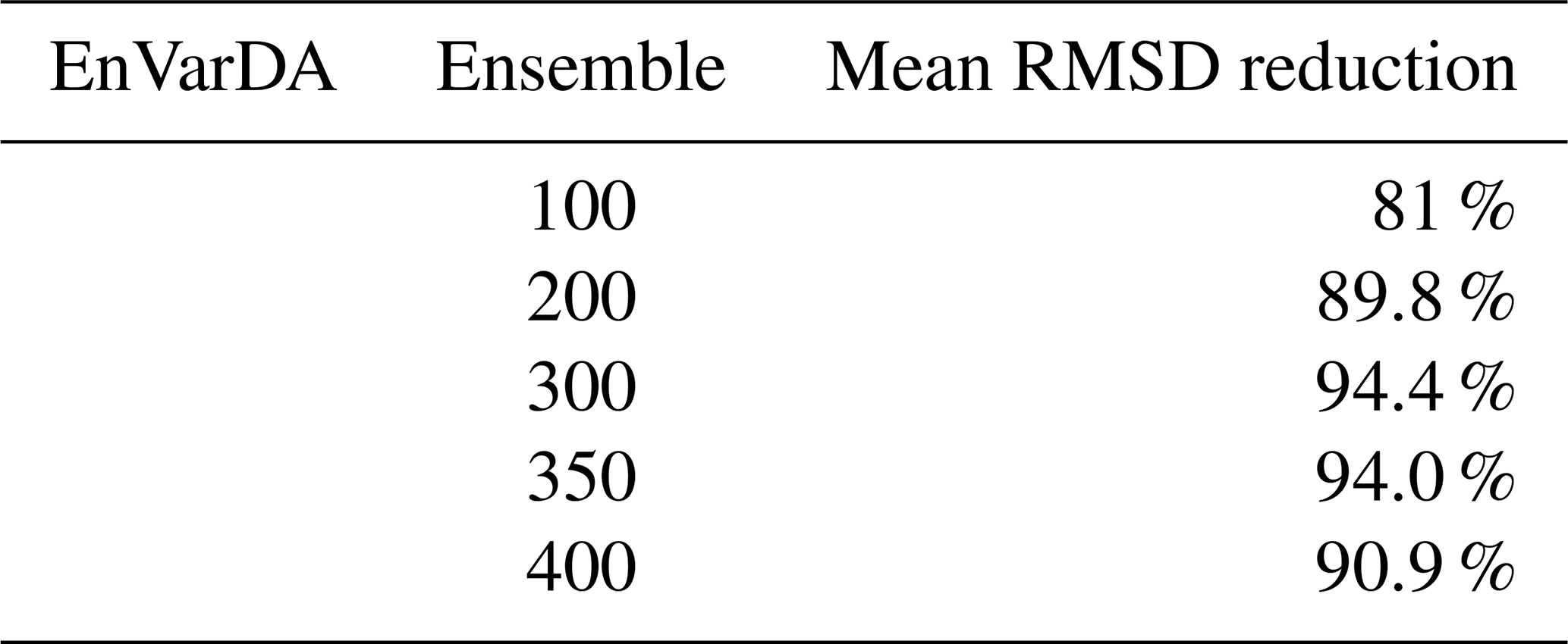
For the complex case, results are presented in Table 2. We see that the best results for the EnVarDA method are obtained with an ensemble of 300 members, giving a mean RMSD reduction of 94.4 %. This configuration is considered for the complex case in Sect. 3.2.2 using the EnVarDA method.

Table 2 Mean RMSD reduction score between synthetic observations and posterior simulations of the atmospheric CO₂ concentration at 21 atmospheric stations for each configuration of the EnVarDA method for the complex case.

3.2 Comparing ϵ-VarDA and EnVarDA

3.2.1 Simple case

Figures 3 and 4 compare the results obtained for the ϵ-VarDA and EnVarDA methods using the configurations chosen in Sect. 3.1. Figure 3 shows that the parameter values obtained by the EnVarDA method are almost equal to the true parameters used to generate the synthetic observations, with a mean absolute difference (MAD) score of 0.3. This shows that the EnVarDA method is able to almost recover the true parameters. The parameter values obtained by the ϵ-VarDA method have a MAD score of 2.05, which reduces the prior MAD by 30 % but remains far from the true parameter values. Only the Vcmax values of PFTs TeNC₃, TeNE, and TrBE are close to the true value of the parameters, whereas PFTs BoNC₃, BoNE, TeBS, TeBE, and TrBR give values that are between the prior and the true value; the Vcmax values of other PFTs have either maintained or increased the distance between the prior and the true values. This shows that the ϵ-VarDA method falls into a local minimum and is therefore unable to recover the true parameters. Figure 4 shows the different RMSD scores between the synthetic observations and prior/posterior simulations for each of the 21 atmospheric stations. The average reduction in RMSD for the ϵ-VarDA method is 82 %, with a mean RMSD of 0.1 ppm. The largest reduction in RMSD is for the German station, Schauinsland (SCH) (87 %), and the lowest is for the Australian station Cape Grim (CGO) (49.8 %). Comparatively, the average reduction in RMSD for the EnVarDA method reaches 97 %, with a mean RMSD of 0.01 ppm across all stations. The highest reduction in RMSD is for the Chinese station, Waliguan (WLG) (99 %), and the lowest is for the Australian station Cape Cleveland (CFA) (92.7 %). We see that the EnVarDA method outperforms the ϵ-VarDA method: the EnVarDA method has the best fit to the assimilated synthetic observations and can find the value of the true parameters used to generate the synthetic observations.

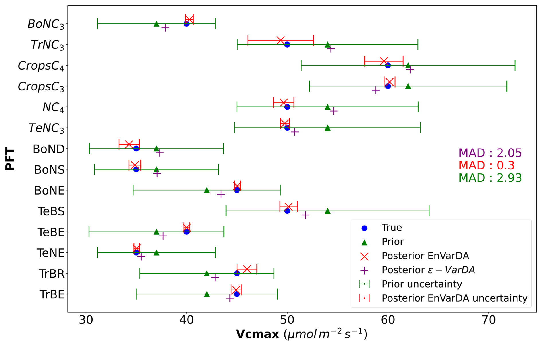
Figure 3 Results in parameter space for the simple case: the prior parameter values are represented by the green triangles, and the posterior parameter values after optimisation are represented by the purple + symbol for the ϵ-VarDA method and the red × symbol for the EnVarDA method. The blue circles represent the true values used to produce the assimilated synthetic observations. The green error bar represents the prior uncertainty, which is also equal to the standard deviation of the prior ensemble used for EnVarDA. The red error bar represents the standard deviation of the posterior ensemble obtained by EnVarDA, which can be interpreted as the posterior uncertainty. The mean absolute difference (MAD) score shown is calculated between the true parameter values used to generate the synthetic observations and the different parameter values following the same colour code (green score using the prior parameter, purple score using the posterior parameter of ϵ-VarDA, and red score using the posterior parameter of EnVarDA).

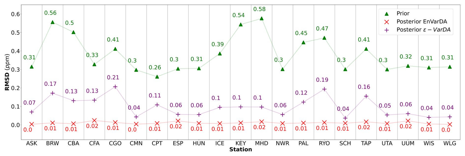
Figure 4 The root mean squared difference (RMSD) scores between synthetic observations and prior simulations for the simple case for each of the 21 atmospheric stations are represented by green triangles. The RMSD scores between synthetic observations and posterior simulations given by the ϵ-VarDA (EnVarDA) method are represented by the purple + symbol (red × symbol).

3.2.2 Complex case

For the complex case, Fig. 5 shows the prior/posterior RMSD at each atmospheric station for the EnVarDA method using an ensemble of 300 members and the ϵ-VarDA method using an ϵ of $\mathrm{5}\times {\mathrm{10}}^{-\mathrm{2}}$ for all parameters. We stop the ϵ-VarDA method after 25 iterations, which already represents 1450 model simulations, as it shows no significant improvement in the minimisation of its cost function. We find that EnVarDA gives a mean reduction in RMSD of 94.3 % across all stations, with a maximum reduction in RMSD at the South African station, Cape Point (CPT) (98.8 %), and a minimum RMSD reduction at the Finland station, Pallas (PAL) (85 %). The ϵ-VarDA method gives a mean reduction in RMSD of 92.5 % across all stations, with a maximum reduction in RMSD at the Chinese station, Walinguan (WLG) (96.9 %), and a minimum RMSD reduction at the Australian station Cape Grim (CGO) (81.3 %). The average RMSD drops from 3.35 to 0.17 ppm after assimilation for EnVarDA and to 0.24 ppm for ϵ-VarDA. Since the posterior RMSDs obtained were close, we performed a paired t test (Student, 1908) between the two posterior RMSDs to determine whether they were significantly different. We obtained a t value of −2.125 between the posterior RMSDs obtained by EnVarDA and ϵ-VarDA, with a p value of 0.046. This confirms that the average posterior RMSD obtained by EnVarDA is significantly lower than the posterior RMSD obtained by ϵ-VarDA, with a confidence level of 95 %. We computed the mean squared difference (MSD) between the synthetic observations concatenated across all stations, the prior simulation, and the two posterior simulations. Following Hodson et al. (2021) and Geman et al. (1992), we decomposed the MSD into bias and variance terms, as presented in Appendix A. The prior MSD is 11.49 ppm² and is reduced to 0.04 ppm² using the EnVarDA method and to 0.08 ppm² using the ϵ-VarDA method. The decomposition of the prior MSD indicates a squared bias of 4.96 ppm² and an error variance equal to 6.53 ppm². The same decomposition for the posterior simulations yields a squared bias of 0.006 ppm² and an error variance equal to 0.03 ppm² for the EnVarDA method and a squared bias of 0.002 ppm² and an error variance equal to 0.07 ppm² for the VarDA method. We calculate the MAD score between the true parameter and the prior/posterior parameters after normalising between 0 and 1 (because the parameters do not have the same units). This normalisation allows us to bound the MAD score between 0 and 1. The normalised MAD score between the true parameters and the prior parameters is 0.17. After assimilation using EnVarDA, a 53 % reduction in this score is obtained, giving a normalised MAD score of 0.08. The ϵ-VarDA method gives a reduction in the normalised MAD of 15 %, giving a normalised MAD score of 0.14. Figure 6 shows the prior, true, and posterior parameter values obtained using both methods. For each parameter, we calculate the MAD score independently. The EnVarDA method gives a MAD reduction of 44.7 % for Vcmax, 78.2 % for SLA, 36.3 % for LAI_max, and 54.2 % for m_maint.resp and a reduction in the absolute difference (AD) of 98.8 % for Q₁₀. The ϵ-VarDA method gives a MAD reduction of 11.3 % for Vcmax, 32.7 % for SLA, 9.6 % for LAI_max, and 4.2 % for m_maint.resp and a reduction in the AD of 97.5 % for Q₁₀.

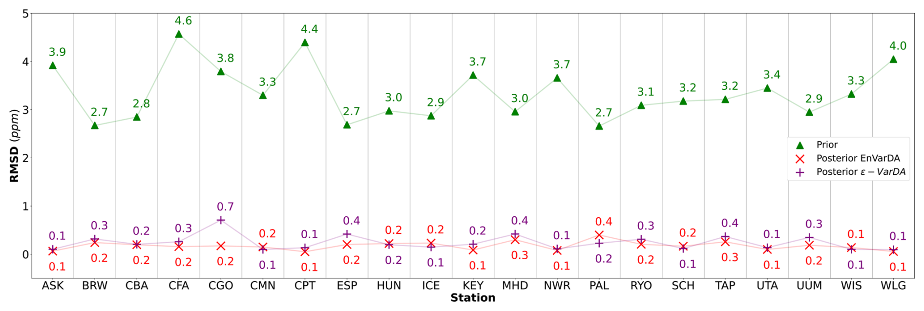
Figure 5 The root mean squared difference (RMSD) scores between synthetic observations and prior simulations for each of the 21 atmospheric stations for the complex case are represented by green triangles. The RMSD scores between synthetic observations and posterior simulations given by the ϵ-VarDA (EnVarDA) method are represented by the purple + symbol (red × symbol).

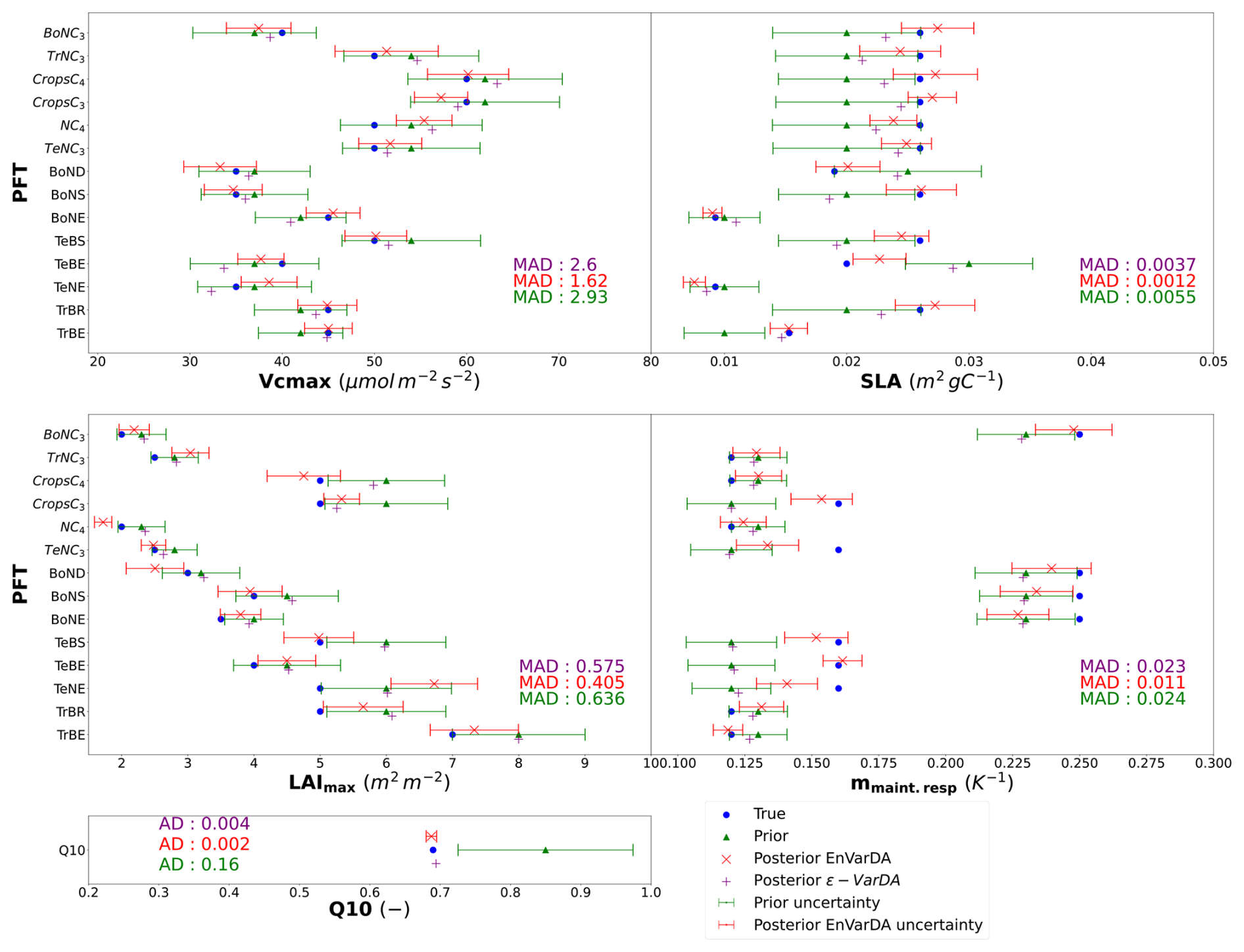
Figure 6 Results in parameter space for the complex case: the prior parameter values are represented by the green triangles, and the posterior parameter values after optimisation are represented by the purple + symbol for the ϵ-VarDA method and the red × symbol for the EnVarDA method. The blue circles represent the values used to produce the assimilated synthetic observations. The green error bar represents the prior uncertainty, which is also equal to the standard deviation of the prior ensemble used for EnVarDA. The red error bar represents the standard deviation of the posterior ensemble obtained by EnVarDA, which can be interpreted as the posterior uncertainty. The MAD (or the absolute differences for Q₁₀) scores shown are calculated for each parameter independently.

Figure 7 illustrates the spatial disparities in net land carbon fluxes between the synthetic fluxes and the prior/posterior estimation of the two methodologies, in addition to their mean annual global net carbon flux. The EnVarDA method achieved a mean annual global net flux of −2.62 Gt C yr⁻¹, with a difference of 0.05 Gt C yr⁻¹ compared to the synthetic fluxes. Spatial differences were limited to an absolute maximum of 0.28 g C m⁻² d⁻¹, with an absolute mean of 0.009 g C m⁻² d⁻¹. In contrast, the ϵ-VarDA method produced a mean annual global net flux of −2.43 Gt C yr⁻¹, with a difference of 0.24 Gt C yr⁻¹ relative to the synthetic fluxes. Spatial differences for this method reached an absolute maximum of 0.6 g C m⁻² d⁻¹, with an absolute mean of 0.031 g C m⁻² d⁻¹. The Pearson correlation coefficient between the synthetic NBP and the prior NBP is 0.87 in time and 0.17 in space. The posterior NBP obtained by the EnVarDA method shows a Pearson correlation coefficient against the synthetic NBP of 0.99 in time and 0.98 in space. In comparison, the posterior NBP obtained by the ϵ-VarDA method has correlation coefficients of 0.98 in time and 0.84 in space.

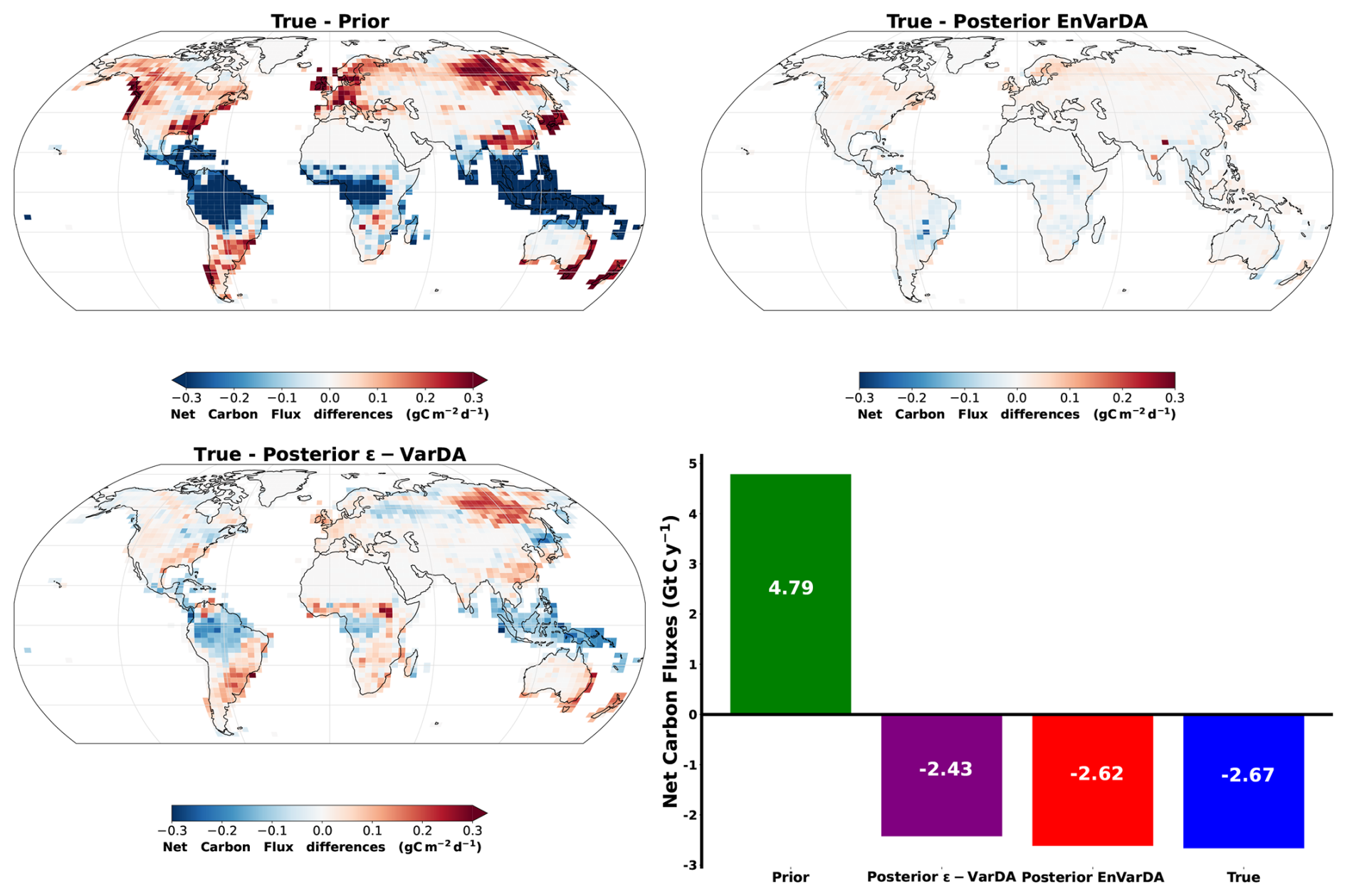
Figure 7 Spatial differences in net land carbon fluxes between synthetic fluxes and the prior/posterior estimate of the two methods alongside their mean annual global net carbon flux for the complex case. (Negative values are carbon uptakes, and positive values are carbon emissions.)

4 Discussion

4.1 Experiments

In Sect. 3.2.1, we found that the EnVarDA method outperforms the ϵ-VarDA method in terms of both RMSD reduction and MAD score, while requiring a smaller number of model simulations for the simple case. The EnVarDA method reduces the RMSD by 97 % and almost recovers the true parameters, whereas the ϵ-VarDA method reduces the RMSD by 82 % and seems to converge into a local minimum. In addition, EnVarDA requires 3 times fewer simulations. The other configurations presented in Sect. 3.1 show that EnVarDA using 50 members leads to similar RMSD reduction to ϵ-VarDA (see Table 1). However, this EnVarDA configuration still gives a better MAD score of 0.44, giving a reduction in the prior MAD by 85 % – this shows that the EnVarDA method is less influenced by local minima than the ϵ-VarDA method. We can also note that using the ϵ-VarDA method results in a posterior parameter values that either (i) remain close to the a priori values or (ii) increase the distance from the value of the true parameters. The first case can be explained by the lower sensitivity of the parameters concerned. The sensitivity of the Vcmax parameter depends on the associated PFT. Not all PFTs have the same impact on NBP fluxes, as they do not have the same spatial distribution or the same proportion (see Table A1). This is the case for the parameters of PFTs TeBE, BoNS, BoND, CropsC₄, and TrNC₃, which have a proportion equal to or less than 3% and are therefore less influential in global NBP fluxes. The second case can be explained by self-compensation due to the equifinality of the problem. Indeed, as some parameters are not properly calibrated, others compensate and may not converge towards the true minimum. It may concern the parameter of PFT NC₄. The EnVarDA method seems to be less affected by these problems and is therefore a promising solution. Furthermore, Fig. 3 shows a significant decrease in the standard deviation of the posterior ensemble. This allows us to identify which parameters and therefore which PFTs appear more sensitive. In this case, it seems that the results for the TrNC₃ and CropsC₄ PFTs are the most uncertain.

In Sect. 3.2.2, we saw that the EnVarDA method is able to calibrate 57 parameters and reduces the mean RMSD by 94.3 %, which is slightly better than the ϵ-VarDA method, with a mean RMSD reduction of 92.5 %. It is worth noting that the mean RMSD reduction may be better in the complex case than in the simple case. This is mainly due to the fact that the a priori error is much larger in the complex case. Nevertheless, the mean RMSD score remains bigger than in the simple case (0.17 and 0.24 ppm for the complex case and 0.01 and 0.1 ppm for the simple case for EnVarDA and ϵ-VarDA, respectively). Furthermore, the MSD score is better for the EnVarDA method (0.04 ppm² using the EnVarDA method and 0.08 ppm² using the VarDA method), and the MSD decomposition (Geman et al., 1992; Hodson et al., 2021) highlights that EnVarDA better reduces the error variance, whereas the squared bias reduction is slightly better for the ϵ-VarDA method. However, squared bias values below 0.01 ppm² are negligible. While the mean RSMD reduction and MSD scores are similar for the complex case, the MAD scores in parameter space are different. In fact, the EnVarDA method is closer to the true parameters by reducing the normalised MAD by 53 %, whereas the ϵ-VarDA method remains very close to the a priori position. The posterior ensemble generated for EnVarDA also shows a reduction in uncertainty for all parameters. This uncertainty reduction is not equal for all parameters – a maximum reduction can be seen for the Q₁₀ parameter (reducing the standard deviation by 94 %) and the lowest for the less sensitive m_maint.resp parameter (with a 14 % reduction for the NC₄ PFT). Both methods are capable of recovering the true Q₁₀ parameter since it is the most sensitive parameter. The ϵ-VarDA method seems to have difficulties in calibrating the parameters m_maint.resp and LAI_max, showing reductions in MAD scores that are less than 10 %. Considering Fig. A2, we can see that some PFTs give partial derivatives that do not completely converge, with an ϵ of 10⁻² (for example, the PFT CropsC₄), so it is likely that ϵ for these parameters is underestimated. Other PFTs seem to give partial derivatives that do completely converge, with an ϵ of 10⁻² (for example, the PFT TrBE), but remain close to their a priori value, so it is likely that the sensitivity of these parameters is low. The other parameters are therefore self-compensating, and this may partly explain the poorer performance of this method in terms of the MAD score, which is always better for the EnVarDA method. The self-compensating effect is illustrated in Fig. 7. The posterior spatial distributions of net carbon flux obtained from the two methods exhibit notable differences. It appears that the ϵ-VarDA method obtains a different spatial structure of the net carbon fluxes. Indeed, the carbon fluxes absent from one region can be reallocated to another, resulting in only minor variations in atmospheric CO₂ concentrations. We believe that the different spatial structure obtained by ϵ-VarDA against the synthetic net carbon flux is likely to be explained by the fact that the two PFTs TrBE and BoND are not well monitored, creating a dipole in the Amazonian and Siberian regions to compensate for the erroneous carbon flux in other regions. It is therefore notable that the EnVarDA method demonstrates superior performance, as it is more aligned with the synthetic net carbon fluxes both spatially and globally compared to the ϵ-VarDA method. Figure A3 shows the differences in the spatial distribution of gross primary production (GPP) between the synthetic fluxes and the prior/posterior estimate of the two methods, as well as their global yearly budget. We can see that GPP obtained with the EnVarDA method is slightly better than that of the ϵ-VarDA method for the global budget and better matches the spatial distribution of the synthetic flux. The ϵ-VarDA method appears to compensate for the lack of change between the prior and posterior GPP across most of the Northern Hemisphere. However, the EnVarDA method also outperforms the ϵ-VarDA method in terms of computational cost: the EnVarDA method only needs 300 simulations, whereas the ϵ-VarDA method needs 1450, which means a reduction in computing time of almost 5 times. This experiment of calibrating a large number of parameters represents a more realistic case, even if we consider a very low model/observation error. The results demonstrate the good performance of EnVarDA, which, even in a “perfect” model situation, i.e. a model that can perfectly simulate observations, can assimilate observations while being less impacted by local minima. However, this may not be the case when using actual observations and introducing more complex modelling/observation errors. The use of EnVarDA here therefore demonstrates its ability to calibrate many parameters with fewer model simulations. In this experiment, one simulation took 11 min on average (wall time), using 20 CPUs of a computer server (with an Intel Xeon Gold 5115 processor). Neglecting the other computational times, using ϵ-VarDA for the complex case represents more than 265 h of computation compared with only 55 h for EnVarDA. Such a reduction cannot be ignored, especially since a simulation in this experiment represents a short (only 2 years), low-cost model configuration – low ORCHIDEE spatial resolution and the use of pre-calculated LMDZ transport fields.

In this twin experiment, both methods have to deal with the inherent equifinality of atmospheric concentration assimilation. This equifinality occurs when parameters compensate for each other, resulting in either an incorrect spatial distribution of NBP or inaccurate estimates of subcomponents, such as GPP and total ecosystem respiration (TER), but still allowing for a match with observations. Although both methods considered in this study successfully recovered the global budgets for NBP and GPP, the ϵ-VarDA method did not obtain the correct spatial distributions of NBP and GPP (see Figs. 7 and A3). This is not the case for the EnVarDA method, which better recovered the true spatial distributions of NBP and GPP. We believe that this equifinality could increase the number of local minima, further disrupting the performance of the ϵ-VarDA method. We also believe that the ensemble nature of the EnVarDA method provides a more comprehensive view of the parameter space, making it less sensitive to local minima and therefore to equifinality issues.

The poorer performance of the ϵ-VarDA method is likely related to inaccurate determination of ϵ, which results in inaccurate estimates of the tangent linear and adjoint models. The EnVarDA method avoids the development and maintenance of tangent linear and adjoint models and ensures a fully functional assimilation method that does not require the use of finite differences. However, the performance of the EnVarDA method seems dependent on the generated ensemble. As shown in Table 2, slightly lower performance is observed with larger ensembles, indicating that a bigger ensemble does not necessarily yield better results. This could be due to the increased dimensionality of the problem, making the iterative minimisation more challenging. Additionally, we generated a new ensemble for each experiment, which provides different information about the parameter space and can lead to different optimal values. This shows the importance of the prior ensemble generated. Nevertheless, the reduction in RMSD remains satisfactory, with a reduction of more than 90 %. It seems that the subjective choice of the EnVarDA setup, i.e. the size and distribution of the ensemble, is less critical than the subjective choice of ϵ used in ϵ-VarDA, which must be determined independently for each of the parameters and given assimilated data streams (with the associated number of model simulations). Moreover, like the tangent linear and adjoint models, this ϵ must be re-tuned for a different model as the sensitivity of the parameter can be different. Indeed, other studies using different versions of the ORCHIDEE LSM used different ϵ values (Santaren et al., 2007; Kuppel et al., 2012; Peylin et al., 2016; Bacour et al., 2023).

The results obtained here for ϵ-VarDA are not equivalent to a standard VarDA method using tangent linear and adjoint models. Therefore, we can draw no conclusions on the comparison between the EnVarDA method and a standard VarDA method, as highlighted in Liu et al. (2008). A potential – but hard to implement – way to improve ϵ-VarDA may be to have a dynamic ϵ that becomes more refined as the methods converge. Nevertheless, even with the “perfect” ϵ, we cannot guarantee that the ϵ-VarDA method would be less computationally expensive. The assimilation of atmospheric CO₂ concentration data using VarDA has been implemented with a tangent linear model, as in Castro-Morales et al. (2019), and an adjoint model, as in Scholze et al. (2007). In these cases, the tangent linear and adjoint models were developed alongside the forward model. However, the ϵ-VarDA method was used in experiments where obtaining the tangent linear or adjoint model proved too difficult, such as in Peylin et al. (2016) and Bacour et al. (2023). Although ϵ-VarDA is not equivalent to standard VarDA, a comparison of EnVarDA with ϵ-VarDA demonstrates the strong performance of EnVarDA, making it a promising candidate for this application.

4.2 Challenges and perspectives

This study relies on twin experiments, which eliminate the complexities associated with model/observation errors and allow us to focus on the performance of two assimilation methods. This experiment highlights the superiority of the EnVarDA method in assimilating atmospheric CO₂ concentration data. However, the assimilation of real observations is not straightforward. The use of real data must be followed by characterisation of the model/observation errors. Indeed, the matrix R must reflect modelling/observation errors at each site, which would introduce spatial heterogeneity, as each station may have different modelling errors, mainly structural errors from both the transport model and the fluxes given by the ORCHIDEE LSM, or measurement problems. A good characterisation of the matrix R is of paramount importance, as it can have a considerable impact on the results obtained. If the model/observation errors are incorrect, the EnVarDA method can give infeasible posterior parameter values, i.e. outside the imposed parameter boundaries, and therefore give non-physical parameter values. Furthermore, even with feasible posterior parameter values, the parameters obtained may be beyond the assumption of linearity made by the use of linear combinations in Eq. (18) and therefore do not improve the associated simulation. Nevertheless, several techniques seem promising for managing these limitations. The inclusion of a weight factor in the background term, as is done in Raoult et al. (2016), and a better definition of the error covariance matrix B may provide a solution. Some of these challenges are not specific to the EnVarDA method and are common to the VarDA method (Raoult et al., 2024b). These challenges are therefore the subject of active research to improve the assimilation of real observational data.

The assimilation of real observations of atmospheric concentrations may also increase the equifinality mentioned in Sect. 4.1 for several reasons, such as (i) incorrect initial conditions of the carbon pools, which can impact respiration; (ii) wrong estimates of other flux components, such as ocean or fossil fuel components; and (iii) structural errors in either the land surface model or the transport model. The issue of incorrect initial conditions can be addressed by starting the simulation a couple of years before the assimilation window. This allows for the correction of the initial carbon pool and better accounts for the effects of the new parameter values on the carbon pool. To handle other components, such as ocean components, the same assimilation can be repeated using different estimates of the ocean flux. Ideally, an ocean model could be included in the optimisation to calibrate both land and ocean components, as is done in atmospheric inversion. The advantage of the EnVarDA method is that it only requires forward simulations. Therefore, no code adaptations are needed, making it easier to use different transport models. This should help detect and address structural errors. The equifinality can also be reduced by assimilating multiple data streams simultaneously, as is done in Peylin et al. (2016) and Bacour et al. (2023), to calibrate both GPP and NBP at the same time.

This study acts as a proof of concept for the assimilation of atmospheric CO₂ concentration data using adjoint-free methods. The next steps for the future would be to use real observations, which come with other technical and scientific problems (e.g. quantifying the model/observation error). Future studies should focus on the assimilation of more recent and more spatially distributed atmospheric CO₂ concentration data – e.g. satellite XCO₂ products – using EnVarDA. To do so, a more recent version of LMDZ and/or ORCHIDEE should be used. Those studies will focus on the processes involved in the carbon cycle to improve their parameterisation and/or to detect any missing processes in the model. As the EnVarDA method only requires forward simulations of the models, it is easy to change the model (either the LSM or the atmospheric transport model). Furthermore, the method is easy to parallelise as each element of the ensemble is independent. Once built, no further call of the model is necessary (except in the analysis step), which allows us to explore different configurations – e.g. in the construction of the error matrix R or the weighting of background terms, both of which play a key role in the assimilation of real observations – without additional computational cost.

Despite extensive research on the automatic generation of tangent linear and adjoint models – either using new languages or differential software – it remains an enormous challenge to acquire and maintain tangent linear and adjoint models for complex and continuously evolving models. However, it is still a key priority to understand structural errors, to quantify uncertainties, and to refine future predictions via parameter calibration. The use of adjoint-free data assimilation methods such as EnVarDA is therefore an excellent opportunity, as it can be implemented quickly and requires no model modification.

Moreover, the EnVarDA method has been used to assimilate several types of data using either a simple carbon model (Douglas et al., 2025) or more complex LSMs such as the JULES LSM (Pinnington et al., 2020, 2021; Cooper et al., 2021). This new application in the ORCHIDEE LSM shows that this method is model independent. By adding different observation terms (one term per data flux) to the cost function, the method should be able to perform multi-flux data assimilation, which would help to reduce the equifinality problem.

5 Conclusions

We have shown that the EnVarDA method has good potential for calibrating ORCHIDEE parameters by assimilating atmospheric CO₂ concentration data and using the LMDZ atmospheric transport model. The method was tested on a so-called twin experiment using two different cases: (1) a simple case where EnVarDA effectively recovered the true parameter values, whereas the ϵ-VarDA method, despite reducing the RMSD, failed to recover the true parameters, and (2) a complex case where both methods achieved up to a 90 % reduction in RMSD, with EnVarDA showing slightly better performance, including a lower MAD score in parameter space, indicating greater efficiency in parameter recovery and an improved alignment with synthetic net carbon fluxes, both spatially and globally. Additionally, EnVarDA is computationally less demanding and does not require the development or maintenance of tangent linear and adjoint models, facilitating the use of updated model versions without modification. By successfully applying this method to the ORCHIDEE model with a pre-calculated LMDZ transport model, we illustrated its adaptability, making it well suited for other land surface models, whether coupled with atmospheric transport models or not.

Appendix A: Metric calculations

The RMSD and MAD used in these studies are calculated as follows:

$$\begin{array}{}\text{(A1)}& {\displaystyle }& {\displaystyle }\mathrm{RMSD}=\sqrt{{\displaystyle \frac{\mathrm{1}}{N_t}}\sum _{t=\mathrm{0}}^{N_t}{\left(\mathcal{H}{\left({\mathit{x}}_{\mathbf{*}}\right)}_t-{\mathit{y}}_t\right)}^{\mathrm{2}}},\text{(A2)}& {\displaystyle }& {\displaystyle }\mathrm{MAD}={\displaystyle \frac{\mathrm{1}}{n_{\mathrm{param}}}}\sum _{i=\mathrm{0}}^{n_{\mathrm{param}}}|{{\mathit{x}}_{\mathbf{*}}}_i-{{\mathit{x}}_{\mathbf{true}}}_i|,\end{array}$$

where x_* can be either x_b or x_a. The Pearson correlation coefficients were computed using the NumPy Python library with the corrcoef function. The paired t tests were computed using the stats.ttest_rel function from the SciPy library. We use the decomposition of MSD into bias and variance that was proposed by Geman et al. (1992) and presented by Hodson et al. (2021):

$$\begin{array}{}\text{(A3)}& {\displaystyle }& {\displaystyle }\mathit{e}=\mathcal{H}\left(\mathit{x}\right)-\mathit{y},\text{(A4)}& {\displaystyle }& {\displaystyle }\mathrm{MSD}\left(\mathit{e}\right)=\mathbb{E}\left[\mathit{e}\right],\text{(A5)}& {\displaystyle }& {\displaystyle }\mathrm{MSD}\left(\mathit{e}\right)=\left(\mathbb{E}\left[{\mathit{e}}^{\mathrm{2}}\right]-\mathbb{E}[\mathit{e}{]}^{\mathrm{2}}\right)+\mathbb{E}[\mathit{e}{]}^{\mathrm{2}},\text{(A6)}& {\displaystyle }& {\displaystyle }\mathrm{MSD}\left(\mathit{e}\right)=\mathrm{Var}\left(\mathit{e}\right)+\mathbb{E}[\mathit{e}{]}^{\mathrm{2}},\text{(A7)}& {\displaystyle }& {\displaystyle }\mathrm{MSD}\left(\mathit{e}\right)=\mathrm{Var}\left(\mathit{e}\right)+\mathrm{Bias}(\mathit{e}{)}^{\mathrm{2}}.\end{array}$$

Figure A1 Ocean fluxes, biomass burning carbon fluxes, and fossil emissions (2000–2009).

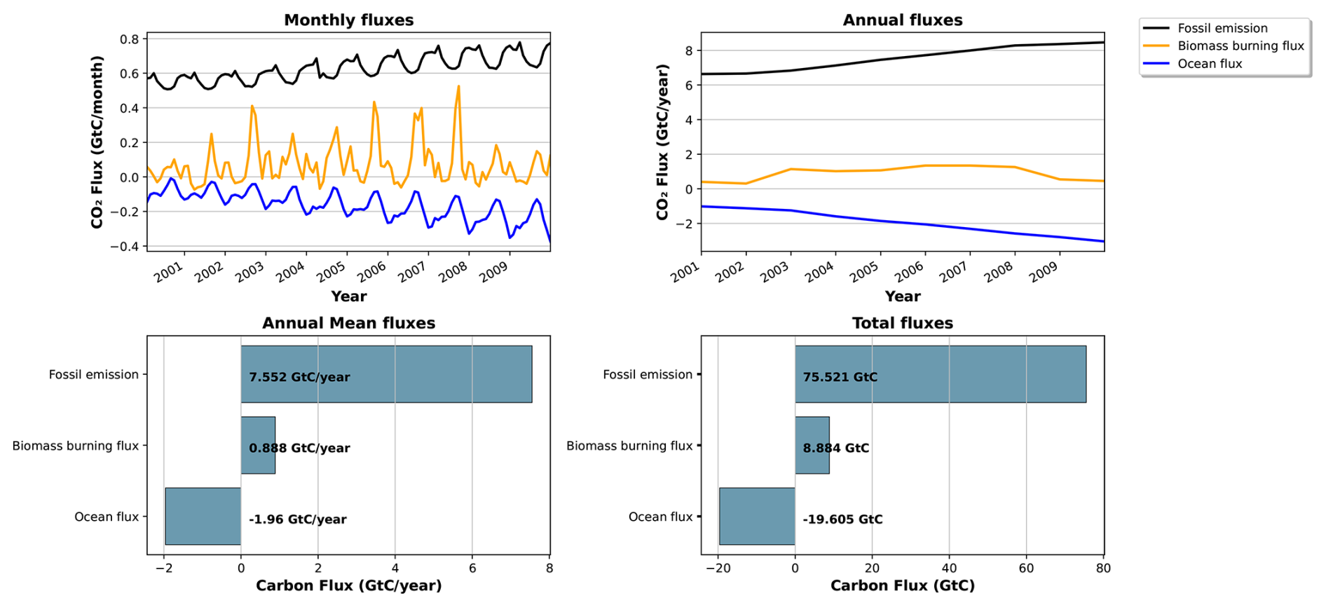
Table A1 Plant functional types (PFTs) in ORCHIDEE with their abbreviations used in this study and their respective global cover fraction (with the remaining portion being bar soil).

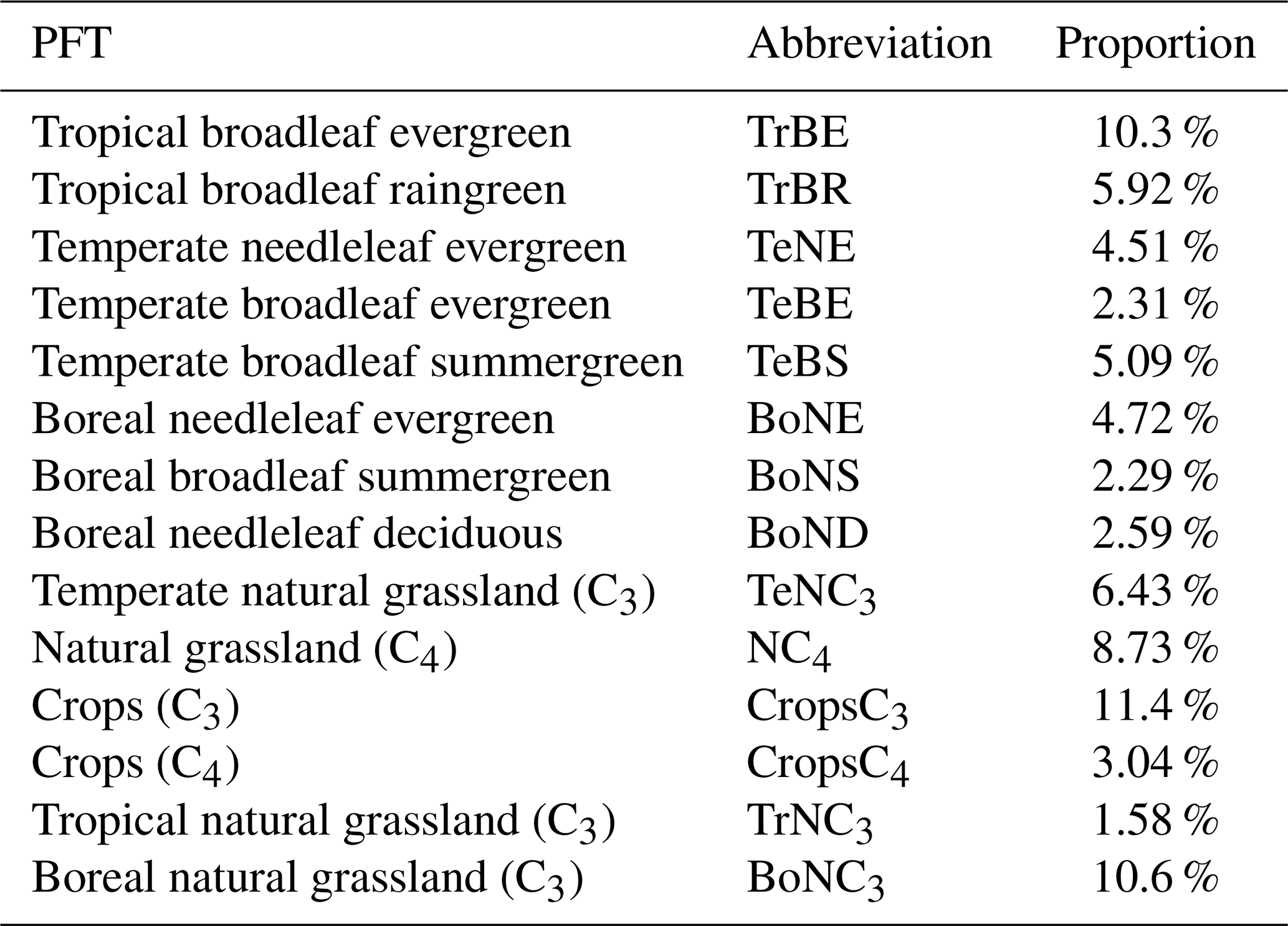
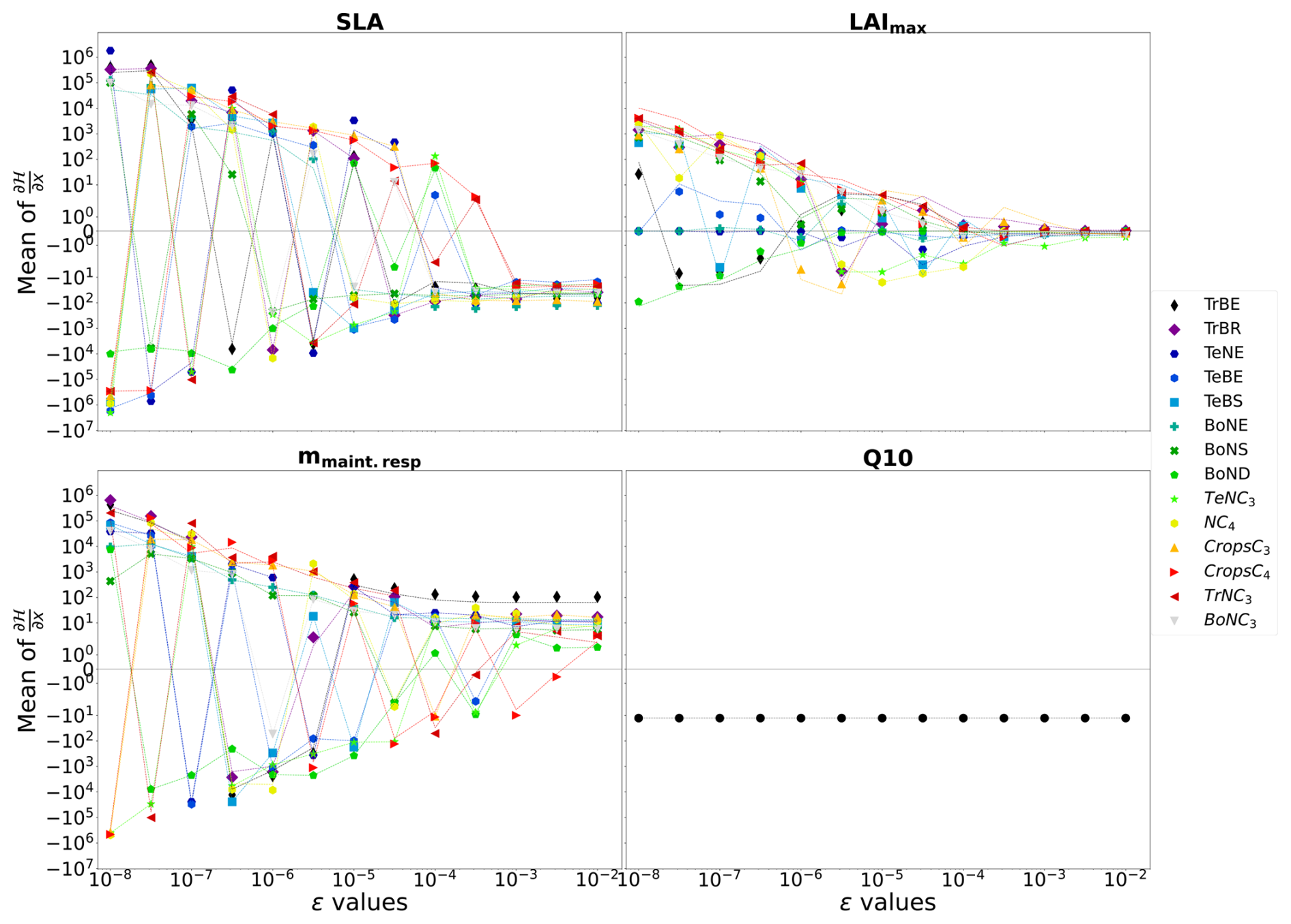
Figure A2 ϵ test: spatial and temporal average of the partial derivative as a function of ϵ. The partial derivative of the 𝓗 model is calculated with respect to the parameters used in the complex case for each PFT. It is calculated on the concentration space using every station over 2 years. The mean of the partial derivative is then calculated over space and time in order to visualise the local derivative. The derivative of 𝓗 is calculated for several ϵ.

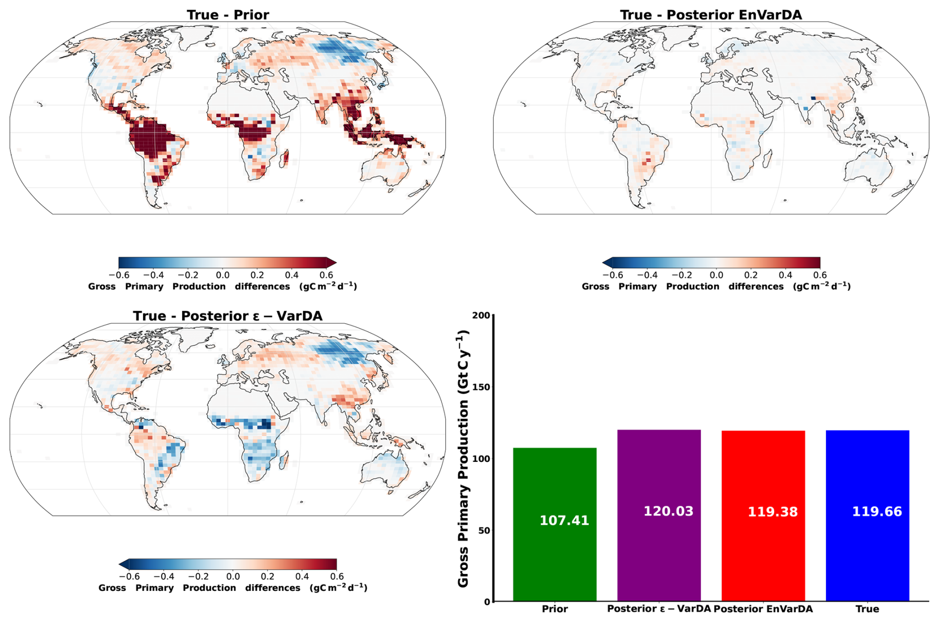
Figure A3 Spatial differences in gross primary production (GPP) fluxes between synthetic fluxes and the prior/posterior estimate of the two methods alongside their mean annual global GPP for the complex case.

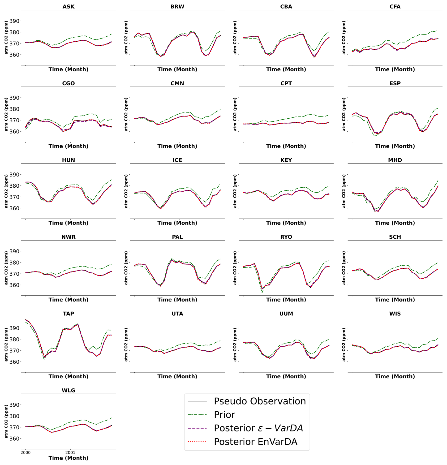
Figure A4 Time series of pseudo-observations (in black) of atmospheric CO₂ concentrations at 21 stations over the assimilated period, as well as the a priori (in green) and a posteriori time series from ϵ-VarDA (in purple) and EnVarDA (in red) for the complex case.

Table A2 Prior value of each parameter and their true values (default values in the ORCHIDEE LSM).

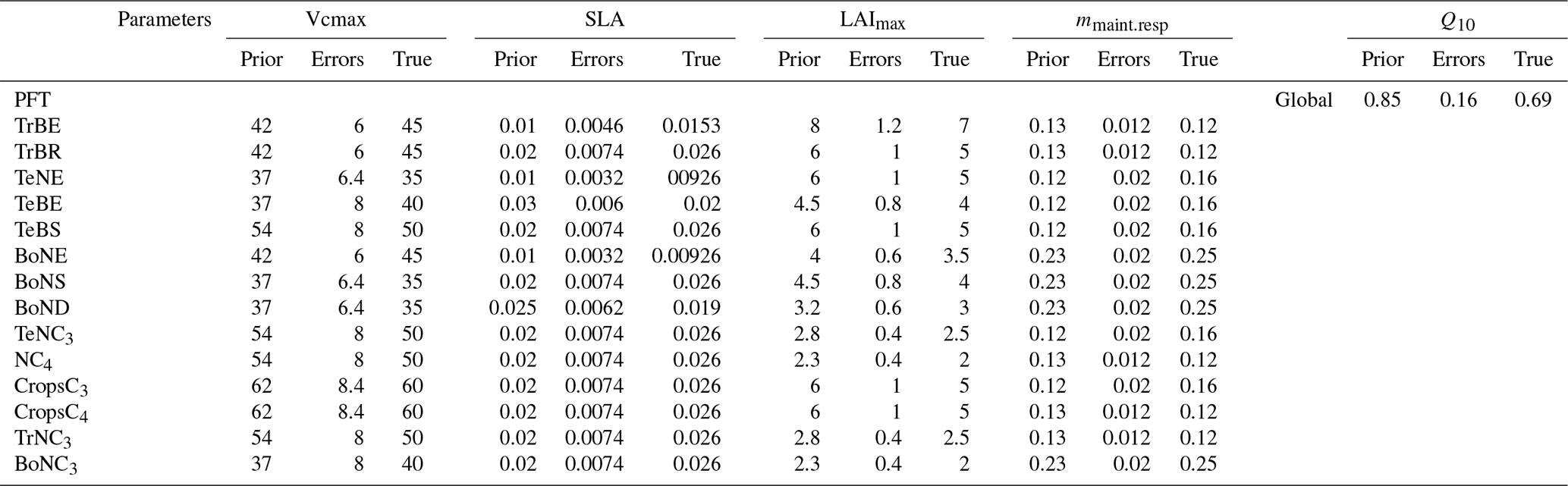
Table A3 Spatial and temporal average of the partial derivative for all parameters for each PFT computed using ϵ, allowing for a stable derivation. The partial derivative is calculated on the concentration space using every station over 2 years. The mean of the partial derivative is then calculated over space and time.