Simple Eulerian–Lagrangian approach to solving equations for sinking particulate organic matter in the ocean

Gravitational sinking of particulate organic matter (POM) is a key mechanism of the vertical transport of carbon in the deep ocean and its subsequent sequestration. The size spectrum of these particles is formed in the euphotic layer by primary production and various mechanisms, including food web consumption. The masses of the particles, as they descend, change under aggregation, fragmentation, and bacterial decomposition. These processes depend on the water temperature and oxygen concentration, particle sinking velocity, ages of the organic particles, ballasting and other factors. In this work, we developed a simple Eulerian–Lagrangian approach to solving equations for sinking particulate matter when the effects of the sizes and ages of the particles, temperature and oxygen concentration on their dynamics and degradation processes are considered. The model considers feedback between the degradation rate and the particle sinking velocity. We rely on known parameterizations, but our Eulerian–Lagrangian approach for solving the problem differs, which enables the algorithm to be incorporated into biogeochemical global ocean models with relative ease. Two novel analytical solutions of a system of one-dimensional Euler equations for the POM concentration and Lagrange equations for the particle mass and position were obtained for constant and age-dependent degradation rates. The feedback between the degradation rate and sinking velocity leads to significant differences in the vertical profiles of the POM concentration and sinking flux, in contrast to the solutions obtained at a constant sinking velocity, where the concentration and flux profiles of the POM are similar. The calculation results are compared with the available measurement data for the POM and POM flux for the latitude bands of 20–30° N in the Atlantic and Pacific Oceans and 50–60° S in the Southern Ocean. The dependence of the degradation rate on temperature significantly affected the profiles of the POM concentration and sinking flux by enhancing the degradation of sinking particles in the ocean's upper layer and suppressing it in the deep layer of the ocean. In all cases considered, the influence of the oxygen concentration was insignificant compared to that of the distribution of temperature with depth.

1 Introduction

Gravitational sinking of particulate organic matter (POM) is a key mechanism of the vertical transport of carbon in the deep ocean (gravitational biological pump) and its subsequent sequestration (Siegel et al., 2023). The biological pump mechanism provides not only the transfer and burial of carbon but also nutrients, trace metals, and natural and artificial radionuclides through a scavenging mechanism (Roca-Martí and Puigcorbé, 2024; De Soto et al., 2018; Maderich et al., 2022). In addition to the processes of sorption and desorption, the mechanism of scavenging is controlled by the sizes of the sinking particles, their densities, the sinking velocity, and the processes of organic particle degradation (Maderich et al., 2021).

The size spectrum of the sinking particles is formed in the euphotic layer by primary production and various mechanisms, including aggregation and fragmentation under the influence of mechanical factors (Burd, 2024) and through food web consumption. The masses of the particles, as they descend in deep layers of the ocean, decrease under the influence of grazing by filter feeders and bacterial decomposition, which depends on the water temperature and oxygen concentration (Cram et al., 2018), particle falling velocity (Alcolombri et al., 2021), ages of the organic particles (Jokulsdottir and Archer, 2016; Aumont et al., 2017) and other factors, such as ballasting (Armstrong et al., 2002; Cram et al., 2018; Maerz et al., 2020). The POM degradation rate can be proportional to the particle mass (volume) (DeVries et al., 2014; Cram et al., 2018) or surface area (Omand et al., 2020; Alcolombri et al., 2021).

Many biogeochemical models assume that the settling velocity of particles is constant or increases linearly with depth (e.g., Aumont et al., 2015). Then, depending on the degradation rate, the vertical profiles of the POM concentration and sinking flux can be determined. At a constant degradation rate, the corresponding vertical profiles of the particle mass concentration and mass flux are exponential (Banse, 1990; Lutz et al., 2002). Assuming that the degradation rate is inversely proportional to the age of the particles (Middelburg, 1989), the vertical profiles of the particle mass concentration and mass flux can be described by a power law (Cael et al., 2021). This power law corresponds to the well-known empirical “Martin curve” (Martin et al., 1987). However, as the particle mass decreases due to degradation, the sinking velocity also decreases. This feedback, along with other factors, is taken into account in several mechanistic models (e.g., DeVries et al., 2014; Cram et al., 2018; Omand et al., 2020; Alcolombri et al., 2021); however, these models do not consider the ages of the particles.

An analytical solution to the equation for the distribution of POM by particle size was obtained by DeVries et al. (2014) for a constant degradation rate. However, as noted by DeVries et al. (2014), the values of the vertical flux of the POM mass at great depths were 1–2 orders of magnitude less than those observed. This discrepancy can be assumed to be due to the constancy of the degradation rate with depth in the model. A decrease in the rate of degradation can also be caused by a decrease in water temperature (e.g., Cram et al., 2018) or an increase in the ages of the sinking particles with depth.

In this work, we developed a simple Eulerian–Lagrangian approach for solving equations for sinking particulate matter when the effects of the sizes and ages of the particles, temperature and oxygen concentration on their dynamics and degradation processes are considered. We relied on known parameterizations (Kriest and Oshlies, 2008; DeVries et al., 2014; Cram et al., 2018), but our Eulerian–Lagrangian approach for solving the problem is different. Our approach involves solving the Euler equation for the concentration of particles of a given size and the Lagrange equations for a sinking organic particle under the influence of microbiological degradation. This enables the incorporation of the proposed algorithm into biogeochemical global ocean models with relative ease. The remainder of the paper is organized as follows: The equations of the model for sinking particulate organic matter are presented in Sect. 2. Analytical solutions for constant and age-dependent degradation rates are obtained and compared with available data on the vertical concentration and mass flux of the POM in Sect. 3. A numerical Eulerian–Lagrangian method for the generalized model is presented in Sect. 4. The results of the simulations are discussed in Sect. 5. Our findings are summarized in Sect. 6. The equivalence of the obtained solution and the solution in (DeVries et al., 2014) for a constant rate of degradation is shown in Appendix A.

2 Model equations

We consider the vertical flux of organic particles caused by gravitational forces. Focusing on the development of a numerical Eulerian–Lagrangian method and finding analytical solutions, we limit ourselves to a fairly simple one-dimensional formulation of the problem away from areas of intense currents. The vertical distribution of these particles below the euphotic layer z_eu is governed by the flux of settling particles equilibrated by particle degradation due to bacterial decomposition. The processes of aggregation, fragmentation and ballasting are not included in the model. We limit ourselves to large-scale climatological processes that cover the water column below the euphotic layer to the bottom. We assume that the effects of time variability on the POM flux are relatively small far from this layer, and we consider the steady states of these fluxes.

The Euler particle concentration transport equation and the Lagrange equations for the individual particles are solved. The Euler equation for the POM spectral concentration C_p,d (unit: mass per volume per particle size increment, kg m⁻⁴) for particles of equivalent spherical diameter d (m) is written as

$$\begin{array}{}\text{(1)}& {\displaystyle \frac{\partial W_{\mathrm{p},d}{C}_{\mathrm{p},d}}{\partial z^{\prime }}}+\mathit{\gamma }{C}_{\mathrm{p},d}=\mathrm{0},\end{array}$$

where W_p,d [m d⁻¹] is the settling velocity of a particle of diameter d, z^′ [m] is the vertical coordinate directed downwards from the depth of the euphotic zone ($z^{\prime }=z-z_{\mathrm{eu}}$), and γ [d⁻¹] is the degradation rate. The boundary condition for Eq. (1) is

$$\begin{array}{}\text{(2)}& z^{\prime }=\mathrm{0}:C_{\mathrm{p},d}=C_{\mathrm{p},d}\left(\mathrm{0}\right),\end{array}$$

where C_p,d(0) is the prescribed POM concentration at the lower boundary of the euphotic layer z_eu.

We consider the particle dynamics in the Lagrangian coordinate system. The porosity of organic particle aggregates increases with increasing particle size (Mullin, 1966). The relationship between the organic matter mass m_d and diameter d of porous particles can be parameterized according to the particle fractal dimension

$$\begin{array}{}\text{(3)}& m_d=c_m{d}^{\mathit{\zeta }}.\end{array}$$

Here, ζ (ζ≤3) is a dimensionless scaling argument, and c_m is a prefactor coefficient (Alldredge and Gotschalk, 1988).

The Stokes-type settling velocity W_p,d depends on the difference between the density of water and the density of the particle, the particle size and shape, and the kinematic viscosity. To consider the entire ensemble of aforementioned factors that impact sinking, we approximate the sinking law by power dependence, which is widely used in particle flux models (e.g., DeVries et al., 2014):

$$\begin{array}{}\text{(4)}& W_{\mathrm{p},d}=c_w{d}^{\mathit{\eta }},\end{array}$$

where η (η≤2) is a dimensionless scaling argument and c_w [m^1−η d⁻¹] is a prefactor coefficient. The measurements of (McDonnell and Buesseler, 2010) show that formulations of sinking velocity as a function of only equivalent particle size can be insufficient because the shapes of the particles (e.g., faecal pellets) can significantly affect the sinking velocity. Figure 1 from (Cael et al., 2021) also demonstrates the difficulties of describing the sinking velocities of particles of various sizes, shapes and structures with a single universal dependence. Therefore, Eq. (4) should be considered only a first approximation when describing the complex dynamics of particles.

We consider the case in which the mass of a particle that is sinking with velocity W_p,d decreases over time t as a result of microbial degradation. This process can be described by a first-order reaction with a reaction rate of γ [d⁻¹]. The corresponding equation for m_d [kg] is written as

$$\begin{array}{}\text{(5)}& {\displaystyle \frac{\partial m_d}{\partial t}}=-\mathit{\gamma }\left(\mathit{\theta }\right)m_d^{\mathit{\theta }},\end{array}$$

Parameter θ=1 when the degradation rate is proportional to the particle mass, and $\mathit{\theta }=\mathrm{2}/\mathrm{3}$ when the degradation rate is proportional to the surface area of the particle (Omand et al., 2020).

In general, the degradation rate depends on many factors. Here, we consider only several of them: the age of the organic particle t [d], the temperature of the sea water T [°C], and the concentration of oxygen [O₂] [μM];

$$\begin{array}{}\text{(6)}& \mathit{\gamma }=\mathit{\gamma }(t,T(z^{\prime }),\left[{\mathrm{O}}_{\mathrm{2}}\right](z^{\prime }\left)\right).\end{array}$$

The parameterization used in Eq. (6) is presented in detail in Sect. 4.

3 Analytical solutions

3.1 Age-independent degradation rate

First, we consider the case in which the degradation rate of the particle is age independent (age-independent degradation rate (AID) model). Furthermore, we suppose that the mass loss is proportional to the mass of the particle (γ=γ₀, θ=1) and does not depend on temperature or oxygen concentration (γ₀=const). Then, the solution of Eq. (5) is

$$\begin{array}{}\text{(7)}& m_d=m_{\mathrm{0}d}\exp (-{\mathit{\gamma }}_{\mathrm{0}}t),\end{array}$$

where $m_{\mathrm{0}d}=c_m{d}_{\mathrm{0}}^{\mathit{\zeta }}$ is the initial value of the particle mass for diameter d₀. Initially, the particle is placed at depth $z^{\prime }=\mathrm{0}$. Combining Eqs. (7) and (3) yields the change in the particle diameter over time as

$$\begin{array}{}\text{(8)}& d\left(t\right)=d_{\mathrm{0}}\exp \left(-{\displaystyle \frac{{\mathit{\gamma }}_{\mathrm{0}}t}{\mathit{\zeta }}}\right).\end{array}$$

Assuming the quasiequilibrium sinking of the particle in the Stokes regime, as described by Eq. (4), and taking into account that particle trajectory in Lagrangian system of coordinates is described as $\partial z^{\prime }/\partial t=W_{\mathrm{p},d}$, we estimate the dependence of the particle depth z^′ on t using Eqs. (4) and (8):

$$\begin{array}{}\text{(9)}& {\displaystyle \frac{\partial z^{\prime }}{\partial t}}=c_w{d}_{\mathrm{0}}^{\mathit{\eta }}\exp \left(-{\displaystyle \frac{\mathit{\eta }{\mathit{\gamma }}_{\mathrm{0}}t}{\mathit{\zeta }}}\right).\end{array}$$

By integrating Eq. (9) from the initial particle depth $z^{\prime }=\mathrm{0}$ at t=0, we find the vertical path travelled by the particle:

$$\begin{array}{}\text{(10)}& z^{\prime }={\displaystyle \frac{\mathit{\zeta }{c}_w{d}_{\mathrm{0}}^{\mathit{\eta }}}{\mathit{\eta }{\mathit{\gamma }}_{\mathrm{0}}}}\left[\mathrm{1}-\exp \left(-{\displaystyle \frac{\mathit{\eta }{\mathit{\gamma }}_{\mathrm{0}}t}{\mathit{\zeta }}}\right)\right].\end{array}$$

By eliminating time from Eq. (8) by using Eq. (10) and then substituting Eq. (8) to Eq. (4), we obtain W_p,d and d as functions of z^′:

$$\begin{array}{}\text{(11)}& {\displaystyle }{W}_{\mathrm{p},d}=H\left(z^{\prime }\right)c_w{d}_{\mathrm{0}}^{\mathit{\eta }}\left(\mathrm{1}-\mathit{\psi }{z}^{\prime }\right),\text{(12)}& {\displaystyle }d=H\left(z^{\prime }\right)d_{\mathrm{0}}{\left(\mathrm{1}-\mathit{\psi }{z}^{\prime }\right)}^{\frac{\mathrm{1}}{\mathit{\eta }}},\end{array}$$

where

$$\begin{array}{}\text{(13)}& \mathit{\psi }={\displaystyle \frac{\mathit{\eta }{\mathit{\gamma }}_{\mathrm{0}}}{\mathit{\zeta }{c}_w{d}_{\mathrm{0}}^{\mathit{\eta }}}}>\mathrm{0}.\end{array}$$

Solutions (11) and (12) describe the vertical distribution of W_p,d and d in the layer of finite thickness $h_{\mathrm{0}}={\mathit{\psi }}^{-\mathrm{1}}$ below which there are only trivial solutions $W_{\mathrm{p},d}=\mathrm{0}$ and d=0. To consider this finding, the Heaviside function is used. The Heaviside function is $H\left(z^{\prime }\right)=\mathrm{1}$ if $z^{\prime }\le {\mathit{\psi }}^{-\mathrm{1}}$ and $H\left(z^{\prime }\right)=\mathrm{0}$ if $z^{\prime }>{\mathit{\psi }}^{-\mathrm{1}}$. Taking into account Eq. (11), we solve Eq. (1) with the boundary condition in Eq. (2) to obtain

$$\begin{array}{}\text{(14)}& C_{\mathrm{p},d}=H\left(z^{\prime }\right)C_{\mathrm{p},d}\left(\mathrm{0}\right){\left(\mathrm{1}-\mathit{\psi }z\right)}^{\frac{\mathit{\zeta }-\mathit{\eta }}{\mathit{\eta }}}.\end{array}$$

The solution (14) describes the vertical profile of the POM concentration for particles of diameter d under the prescribed particle size distribution N(d₀) [m⁻⁴] at $z^{\prime }=\mathrm{0}$. The distribution N(d₀) was approximated in such a way that the number of particles decreased with increasing particle size according to power law scaling

$$\begin{array}{}\text{(15)}& N\left(d_{\mathrm{0}}\right)=M_{\mathrm{0}}{d}_{\mathrm{0}}^{-\mathit{ϵ}},\end{array}$$

where ϵ is a power-law exponent and M₀ is a constant that can be estimated from the total concentration of sinking POM at $z^{\prime }=\mathrm{0}$. The power law distribution is typically observed in the mixed layer (e.g., Kostadinov et al., 2009). Then, the distribution C_p,d(0) can be represented as a product of particle size distribution N(d₀) and mass of particle m_0,d :

$$\begin{array}{}\text{(16)}& C_{\mathrm{p},d}\left(\mathrm{0}\right)=M_{\mathrm{0}}{d}_{\mathrm{0}}^{-\mathit{ϵ}}{m}_{\mathrm{0},d}=M_{\mathrm{0}}{c}_m{d}_{\mathrm{0}}^{\mathit{\zeta }-\mathit{ϵ}}.\end{array}$$

Considering a small increment of particle size Δd₀ we assume that the concentration C_p,d(0) is uniform within the interval Δd₀. The total concentration C_p [kg m⁻³] is calculated as the sum of concentrations C_p,k multipled by increment of particle size Δd₀ in the kth interval over the total number of n_d intervals:

$$\begin{array}{}\text{(17)}& \begin{array}{rl}{C}_{\mathrm{p}}\left(z^{\prime }\right)& =\sum _{k=\mathrm{0}}^{n_d}{C}_{\mathrm{p},k}\mathrm{\Delta }{d}_{\mathrm{0}}=M_{\mathrm{0}}{c}_m\sum _{k=\mathrm{0}}^{n_d}{d}_{\mathrm{0},k}^{\mathit{\zeta }-\mathit{ϵ}}H\left(z^{\prime }\right)\\ & {\left(\mathrm{1}-\mathit{\psi }{z}^{\prime }\right)}^{\frac{\mathit{\zeta }-\mathit{\eta }}{\mathit{\eta }}}\mathrm{\Delta }{d}_{\mathrm{0}},\end{array}\end{array}$$

where $d_{\mathrm{0},k}=k\mathrm{\Delta }{d}_{\mathrm{0}}+d_{\mathrm{0}}^{\min }$, $\mathrm{\Delta }{d}_{\mathrm{0}}=(d_{\mathrm{0}}^{\max }-d_{\mathrm{0}}^{\min })/n_d$, and $d_{\mathrm{0}}^{\min }$ and $d_{\mathrm{0}}^{\max }$ are the minimal and maximal values, respectively, of d₀. At Δd₀→0, the total concentration of sinking POM C_p in the range from $d_{\mathrm{0}}^{\min }$ to $d_{\mathrm{0}}^{\max }$ can be calculated as

$$\begin{array}{}\text{(18)}& C_{\mathrm{p}}\left(z^{\prime }\right)=M_{\mathrm{0}}{c}_m\underset{d_{\mathrm{0}}^{\min }}{\overset{d_{\mathrm{0}}^{\max }}{\int }}{\stackrel{\mathrm{̃}}{d}}_{\mathrm{0}}^{\mathit{\zeta }-\mathit{ϵ}}H\left(z^{\prime }\right){\left(\mathrm{1}-\mathit{\psi }{z}^{\prime }\right)}^{\frac{\mathit{\zeta }-\mathit{\eta }}{\mathit{\eta }}}d{\stackrel{\mathrm{̃}}{d}}_{\mathrm{0}}.\end{array}$$

The total mass flux F_p [kg m⁻² d⁻¹] can be calculated in a similar way:

$$\begin{array}{}\text{(19)}& \begin{array}{rl}{F}_{\mathrm{p}}\left(z^{\prime }\right)& =\sum _{k=\mathrm{0}}^{n_d}{C}_{\mathrm{p},k}{W}_{\mathrm{p},k}\mathrm{\Delta }{d}_{\mathrm{0}}\\ & =M_{\mathrm{0}}{c}_m{c}_w\sum _{k=\mathrm{0}}^{n_d}{d}_{\mathrm{0},k}^{\mathit{\eta }+\mathit{\zeta }-\mathit{ϵ}}H\left(z^{\prime }\right){\left(\mathrm{1}-\mathit{\psi }{z}^{\prime }\right)}^{\frac{\mathit{\zeta }}{\mathit{\eta }}}\mathrm{\Delta }{d}_{\mathrm{0}}.\end{array}\end{array}$$

Here, W_p,k is the sinking velocity in the kth interval of size d over a total of n_d intervals. At Δd₀→0,

$$\begin{array}{}\text{(20)}& F_{\mathrm{p}}\left(z^{\prime }\right)=M_{\mathrm{0}}{c}_m{c}_w\underset{d_{\mathrm{0}}^{\min }}{\overset{d_{\mathrm{0}}^{\max }}{\int }}{\stackrel{\mathrm{̃}}{d}}_{\mathrm{0}}^{\mathit{\eta }+\mathit{\zeta }-\mathit{ϵ}}H\left(z^{\prime }\right){\left(\mathrm{1}-\mathit{\psi }{z}^{\prime }\right)}^{\frac{\mathit{\zeta }}{\mathit{\eta }}}d{\stackrel{\mathrm{̃}}{d}}_{\mathrm{0}}.\end{array}$$

The problem for which we obtained the solution (14) for the POM concentration C_p,d is similar to that solved by DeVries et al. (2014) for the particle size spectrum equation. In Appendix A, we show the equivalence of these solutions.

3.2 Age-dependent degradation rate

The degradation rate as a function of POM age t [d] can be described by following Middelburg (1989) as

$$\begin{array}{}\text{(21)}& \mathit{\gamma }\left(t\right)={\displaystyle \frac{\mathit{\beta }}{\mathit{\alpha }+t}},\end{array}$$

where α [d] and β are empirical constants. We define such a model as an age-dependent degradation rate (ADD) model. The time dependencies of d and $W_{\mathrm{p},d}=\partial z^{\prime }/\partial t$ with parameterization of the degradation rate Eq. (21) are obtained similarly to those in Sect. 3.1. They are expressed as

$$\begin{array}{}\text{(22)}& {\displaystyle }d=d_{\mathrm{0}}{\left({\displaystyle \frac{\mathit{\alpha }}{\mathit{\alpha }+t}}\right)}^{\mathit{\beta }/\mathit{\zeta }},\text{(23)}& {\displaystyle \frac{\partial z^{\prime }}{\partial t}}=c_w{d}_{\mathrm{0}}^{\mathit{\eta }}{\left({\displaystyle \frac{\mathit{\alpha }}{\mathit{\alpha }+t}}\right)}^{\mathit{\eta }\mathit{\beta }/\mathit{\zeta }}.\end{array}$$

Integrating Eq. (23) from the initial particle depth $z^{\prime }=\mathrm{0}$ at t=0, we find the path travelled by a sinking particle as

$$\begin{array}{}\text{(24)}& z^{\prime }=c_w{d}_{\mathrm{0}}^{\mathit{\eta }}{\displaystyle \frac{\mathit{\alpha }\mathit{\zeta }}{\mathit{\zeta }-\mathit{\eta }\mathit{\beta }}}\left[{\left(\mathrm{1}+{\displaystyle \frac{t}{\mathit{\alpha }}}\right)}^{(\mathit{\zeta }-\mathit{\eta }\mathit{\beta })/\mathit{\zeta }}-\mathrm{1}\right].\end{array}$$

By eliminating time from Eqs. (21), (22) and (23), we obtain depth-dependent solutions in the same way as in Eqs. (11)–(12):

$$\begin{array}{}\text{(25)}& {\displaystyle }{W}_{\mathrm{p},d}\left(z^{\prime }\right)=c_w{d}_{\mathrm{0}}^{\mathit{\eta }}{\left(\mathrm{1}+\mathit{\varphi }{z}^{\prime }\right)}^{-\frac{\mathit{\eta }\mathit{\beta }}{\mathit{\zeta }-\mathit{\eta }\mathit{\beta }}},\text{(26)}& {\displaystyle }\mathit{\gamma }\left(z^{\prime }\right)={\displaystyle \frac{\mathit{\beta }}{\mathit{\alpha }}}{\left(\mathrm{1}+\mathit{\varphi }{z}^{\prime }\right)}^{-\frac{\mathit{\zeta }}{\mathit{\zeta }-\mathit{\eta }\mathit{\beta }}},\text{(27)}& {\displaystyle }d\left(z^{\prime }\right)=d_{\mathrm{0}}{\left(\mathrm{1}+\mathit{\varphi }{z}^{\prime }\right)}^{-\frac{\mathit{\beta }}{\mathit{\zeta }-\mathit{\eta }\mathit{\beta }}},\end{array}$$

where

$$\begin{array}{}\text{(28)}& \mathit{\varphi }={\displaystyle \frac{\mathit{\zeta }-\mathit{\eta }\mathit{\beta }}{\mathit{\alpha }\mathit{\zeta }{c}_w{d}_{\mathrm{0}}^{\mathit{\eta }}}}.\end{array}$$

The parameter ϕ [m⁻¹] characterizes the vertical scale of attenuation $W_{\mathrm{p},d}\left(z^{\prime }\right)$, γ(z^′) and d(z^′) with depth.

By integrating Eq. (1) with the boundary condition in Eq. (2) and considering Eqs. (25) and (26), we obtain the following solution for C_p,d:

$$\begin{array}{}\text{(29)}& C_{\mathrm{p},d}\left(z^{\prime }\right)=C_{\mathrm{p},d_{\mathrm{0}}}{\left(\mathrm{1}+\mathit{\varphi }{z}^{\prime }\right)}^{\frac{(\mathit{\eta }-\mathit{\zeta })\mathit{\beta }}{\mathit{\zeta }-\mathit{\eta }\mathit{\beta }}}.\end{array}$$

The density of the distribution of the particle mass concentration at $z^{\prime }=\mathrm{0}$ is assumed to be approximated by a power law (Eq. 15). We can obtain the total concentration of sinking POM C_p in the range of d₀ from $d_{\mathrm{0}}^{\min }$ to $d_{\mathrm{0}}^{\max }$ as

$$\begin{array}{}\text{(30)}& C_{\mathrm{p}}\left(z^{\prime }\right)=M_{\mathrm{0}}{c}_m\underset{d_{\mathrm{0}}^{\min }}{\overset{d_{\mathrm{0}}^{\max }}{\int }}{\stackrel{\mathrm{̃}}{d}}_{\mathrm{0}}^{\mathit{\zeta }-\mathit{ϵ}}{\left(\mathrm{1}+\mathit{\varphi }{z}^{\prime }\right)}^{\frac{(\mathit{\eta }-\mathit{\zeta })\mathit{\beta }}{\mathit{\zeta }-\mathit{\eta }\mathit{\beta }}}d{\stackrel{\mathrm{̃}}{d}}_{\mathrm{0}}.\end{array}$$

The corresponding total mass flux F_p(z) is written as

$$\begin{array}{}\text{(31)}& \begin{array}{rl}{F}_{\mathrm{p}}\left(z^{\prime }\right)& =\underset{d_{\mathrm{0}}^{\min }}{\overset{d_{\mathrm{0}}^{\max }}{\int }}{W}_{\mathrm{p},d}{C}_{\mathrm{p},d}d{\stackrel{\mathrm{̃}}{d}}_{\mathrm{0}}\\ & =M_{\mathrm{0}}{c}_m{c}_w\underset{d_{\mathrm{0}}^{\min }}{\overset{d_{\mathrm{0}}^{\max }}{\int }}{\stackrel{\mathrm{̃}}{d}}_{\mathrm{0}}^{\mathit{\eta }+\mathit{\zeta }-\mathit{ϵ}}{\left(\mathrm{1}+\mathit{\varphi }{z}^{\prime }\right)}^{-\frac{\mathit{\zeta }\mathit{\beta }}{\mathit{\zeta }-\mathit{\eta }\mathit{\beta }}}d{\stackrel{\mathrm{̃}}{d}}_{\mathrm{0}}.\end{array}\end{array}$$

3.3 Comparison of analytical solutions

The obtained analytical solutions have several important properties. First, we compare these solutions with the solutions obtained under the assumption of a constant sinking velocity when

$$W_{\mathrm{p},d}=c_w{d}_{\mathrm{0}}^{\mathit{\eta }}.$$

The solution of Eq. (1) for a constant degradation rate γ corresponds to the exponential profile of the particle concentration

$$\begin{array}{}\text{(32)}& C_{\mathrm{p}}(z^{\prime },d_{\mathrm{0}})=C_{\mathrm{p}}(\mathrm{0},d_{\mathrm{0}})\exp \left(-{\displaystyle \frac{{\mathit{\gamma }}_{\mathrm{0}}{z}^{\prime }}{c_w{d}_{\mathrm{0}}^{\mathit{\eta }}}}\right),\end{array}$$

whereas the time-dependent degradation rate (Eq. 21) corresponds to the power-law distribution of the POM concentration

$$\begin{array}{}\text{(33)}& C_{\mathrm{p}}(z^{\prime },d_{\mathrm{0}})=C_{\mathrm{p}}(\mathrm{0},d_{\mathrm{0}}){\left({\displaystyle \frac{\mathit{\alpha }{c}_w{d}_{\mathrm{0}}^{\mathit{\eta }}}{\mathit{\alpha }{c}_w{d}_{\mathrm{0}}^{\mathit{\eta }}+z^{\prime }}}\right)}^{\mathit{\beta }}.\end{array}$$

Both of these solutions are frequently used to approximate observed particle flux profiles, e.g., (Martin et al., 1987; Lutz et al., 2002). Notably, a solution of the form (Eq. 33) can alternatively be obtained under the assumption of a constant degradation rate and a linear increase in the sinking velocity (Kriest and Oshlies, 2008; Cael and Bisson , 2018).

The corresponding profiles of $C_{\mathrm{p}}(z^{\prime },d_{\mathrm{0}})$ and $F_{\mathrm{p}}(z^{\prime },d_{\mathrm{0}})$ were obtained by summing the n_d profiles in Eqs. (32) and (33) similarly Eqs. (17) and (19). The values of C_p(0,d₀) were calculated using Eq. (16). The model parameters (η, ζ, γ₀, c_w, ϵ, α, β, $d_{\mathrm{0}}^{\max }$, $d_{\mathrm{0}}^{\min }$, and n_d) in Table 1 were the same as in (DeVries et al., 2014) and (Aumont et al., 2017). As shown in Fig. 1, with these parameters, C_p and F_p decay much faster for the AID model than for the ADD model. Notably, C_p and F_p tend to exhibit exponential or power-law profiles only at great depths. Moreover, at a constant particle velocity, the mass-weighted sinking velocity of particles

$${\stackrel{\mathrm{‾}}{W}}_{\mathrm{p}}\left(z^{\prime }\right)={\displaystyle \frac{F_{\mathrm{p}}\left(z^{\prime }\right)}{C_{\mathrm{p}}\left(z^{\prime }\right)}}$$

increases with depth.

Smayda (1970)Mullin (1966)Kriest and Oshlies (2008)Kriest and Oshlies (2008)Kostadinov et al. (2009)Cram et al. (2018)Cram et al. (2018)Cram et al. (2018)Aumont et al. (2017)Aumont et al. (2017)DeVries et al. (2014)DeVries et al. (2014)DeVries et al. (2014)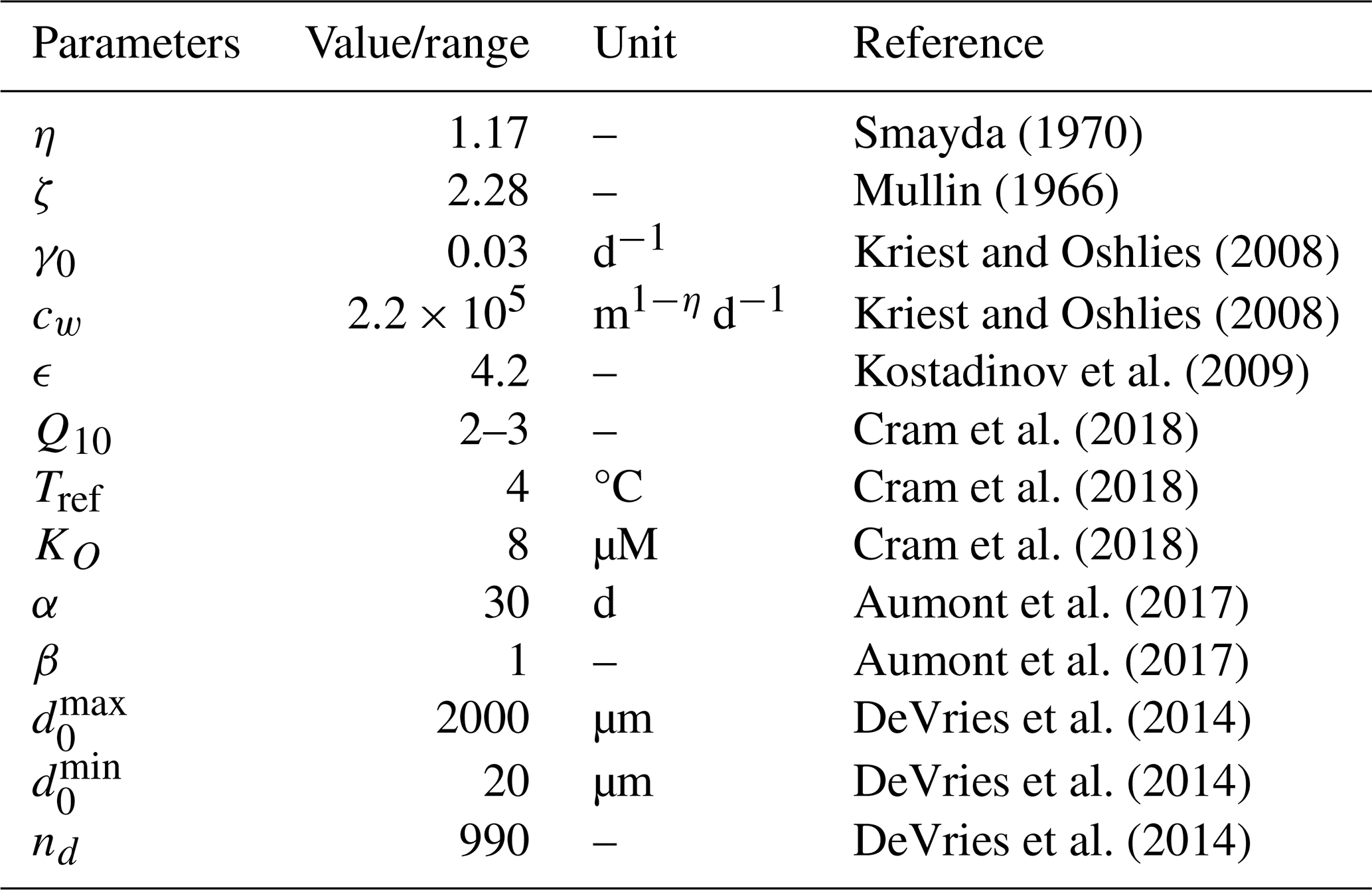

Table 1 Baseline model parameters.

The presence of feedback between γ and W_p,d leads to significant changes in the C_p and F_p profiles. In the case of a constant γ₀, the vertical distribution of the concentration C_p,d for one surface fraction of POM size d₀ is limited by a finite layer of thickness $h_{\mathrm{0}}=\left(\mathit{\zeta }{c}_w{d}_{\mathrm{0}}^{\mathit{\eta }}\right)(\mathit{\eta }{\mathit{\gamma }}_{\mathrm{0}}{)}^{-\mathrm{1}}$. The particles in this layer sink at a linearly decreasing velocity. The masses of the particles also decrease with depth until a depth at which they are completely remineralized is reached. The size distribution for a single class of particles at depth z^′ is $N(d,z^{\prime })=C_{\mathrm{p},d}{m}_d^{-\mathrm{1}}\sim (\mathrm{1}-\mathit{\psi }{z}^{\prime }{)}^{-\mathrm{1}}$. At $z^{\prime }\to h_{\mathrm{0}}$, $N(d,z^{\prime })\to \mathrm{\infty }$ as m_d→0. The finite thickness of the layer of sinking particles with the parameters given in Table 1 varies from 45.4 m at d₀=20 µm to 9937 m at d₀=2000 µm. Notably, the solution to the problem in a different formulation (Omand et al., 2020) has the same qualitative character. However, the total POM concentration and total POM flux decay asymptotically approaching exponential profiles, in contrast to the profiles (14) and (11) for one class of particle sizes d₀ on $z^{\prime }=\mathrm{0}$. The total concentration and flux profiles, normalized to values at the base of the euphotic layer, are shown in Fig. 1, where the C_p and F_p profiles were obtained via the summation of the n_d profiles in Eqs. (17) and (19). The baseline parameters for the calculation are presented in Table 1. These parameter values match those used by DeVries et al. (2014). Therefore, the curves in Fig. 1 also coincide with the corresponding curves in Fig. 1c from (DeVries et al., 2014), which were calculated using an equivalent formulation of the same problem, as shown in the Appendix.

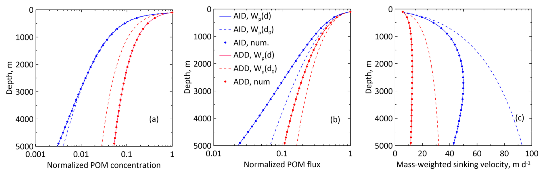
Figure 1 Normalized total POM concentration C_p (a), total POM flux F_p (b), and weighted vertical velocities of the particles (c) for the AID (blue lines) and ADD (red lines) models calculated from the analytical and numerical solutions. The dashed lines correspond to the solutions of Eq. (1) at constant W_p(d₀), whereas the solid line corresponds to the solution of the problem at variable W_p,d. The small circles correspond to the numerical solutions obtained via the AID and ADD models.

In contrast to the AID model solution (17), the POM concentration profile (29) decays asymptotically with depth at ζ>η and ζ>ηβ for the ADD model (21). These conditions are met for the parameters listed in Table 1. The rate of degradation γ also decays with depth. Unlike the models (Kriest and Oshlies, 2008; Cael and Bisson, 2018) that use the same “Martin curve” power-law dependence (Eq. 33) for the concentration and mass flux of POM with the exponent β, the exponent in the obtained solution (29) depends not only on β but also on the parameters that characterize the sinking velocity (η) and the particle mass fractal dimension (ζ).

The sensitivity of the AID model parameters was considered by DeVries et al. (2014). They reported that four parameters (η, ζ, γ₀, and ϵ) control the flux profile and that the most significant factor is the slope of the particle distribution ϵ on $z^{\prime }=\mathrm{0}$, which has the greatest influence on the depth distribution of the particles. In Fig. 2, the variables are presented in logarithmic coordinates. Only the vertical distribution of C_p is close to the power distribution with an exponent of approximately 1, whereas the distribution with depth of F_p significantly deviates from power law (Martin's law). The sensitivity of the concentration and flux profiles to the values of parameters α and β is examined in Fig. 2. An increase in α leads to a deepening of the concentration and particle flux profiles, whereas an increase in β leads to a shallowing of these profiles.

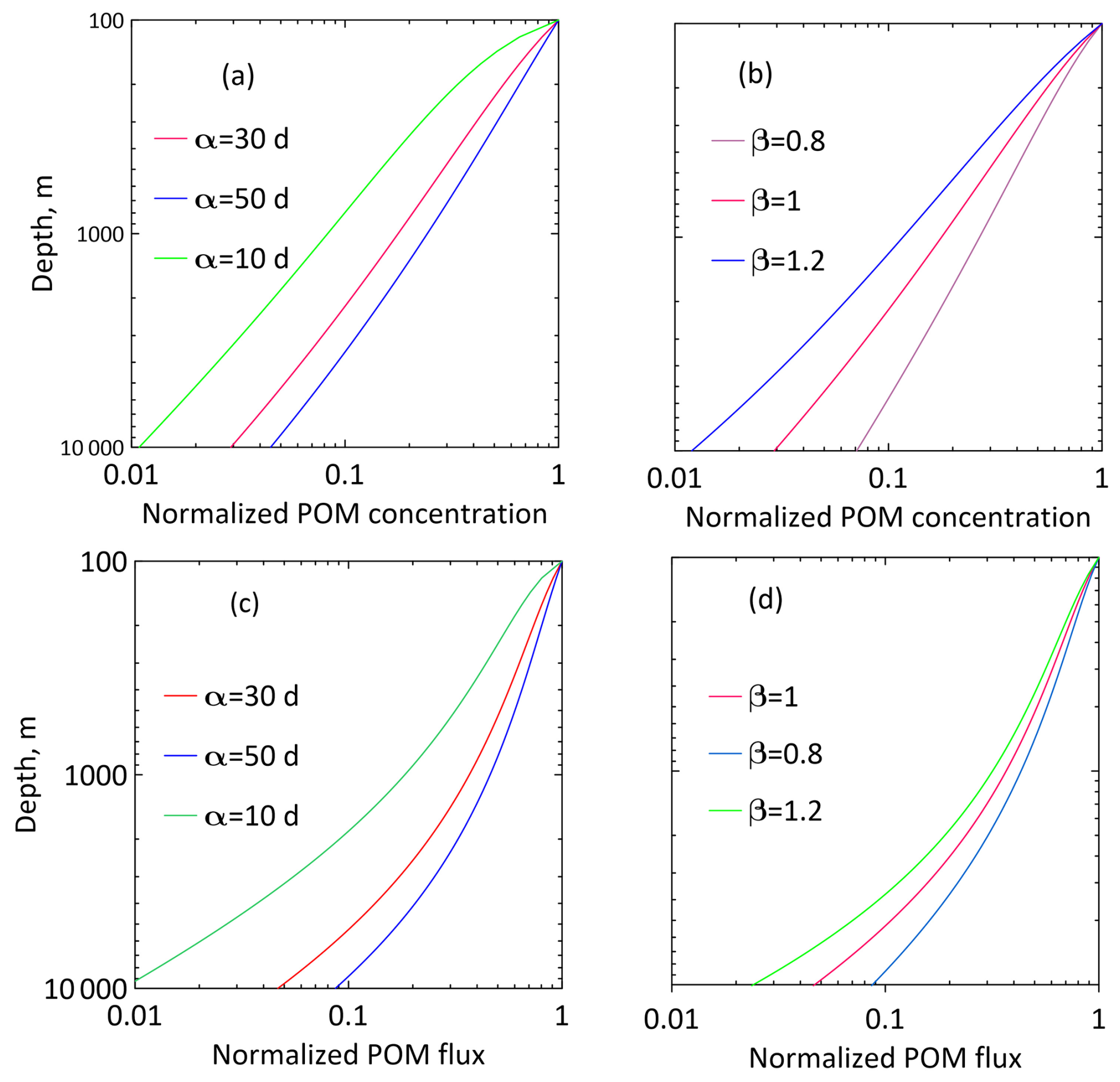
Figure 2 Sensitivity of the normalised total particle concentration C_p (a) and total particle flux F_p (b) to parameters α and β.

The relative maximal absolute errors (%) of the calculated AID and ADD solutions for C_p and F_p are presented in Table S1 in the Supplement. We compare the solutions at spectral resolutions n_d=100 and n_d=10 with the baseline calculation at n_d=990. These estimates demonstrate the necessity of fine resolution of the spectre of particles at the lower boundary of the euphotic zone for obtaining accurate profiles of the POM concentration and sinking flux. In this case, the particle concentration profile is more sensitive to the spectral resolution than the sinking flux profile is.

4 Numerical model

4.1 Numerical algorithm

The model discussed in the previous section is based on several simplifying assumptions that make obtaining analytical solutions to the system of equations possible. However, when we expand the model to include new important factors in the processes of sinking and remineralization of POM, analytical solutions to the problem can no longer be obtained. Therefore, a new numerical Eulerian–Lagrangian approach for solving this problem was developed.

Here, we consider the case in which the degradation rate depends on the age of the organic particle (ADD model), the temperature of the sea water T and the concentration of oxygen [O₂]:

$$\begin{array}{}\text{(34)}& \begin{array}{rl}\mathit{\gamma }& =\mathit{\gamma }(t,T(z^{\prime }),\left[{\mathrm{O}}_{\mathrm{2}}\right](z^{\prime }\left)\right)\\ & =\left({\displaystyle \frac{\mathit{\beta }}{\mathit{\alpha }+t}}\right)\left(Q_{\mathrm{10}}^{\frac{T-T_{\mathrm{ref}}}{\mathrm{10}}}\right)\left({\displaystyle \frac{\left[{\mathrm{O}}_{\mathrm{2}}\right]}{K_{\mathrm{O}}+\left[{\mathrm{O}}_{\mathrm{2}}\right]}}\right),\end{array}\end{array}$$

where Q₁₀ is the temperature coefficient, T_ref is a reference temperature, and K_O [µM] is an oxygen dependence parameter (Cram et al., 2018). When γ does not depend on age (AID model), then

$$\begin{array}{}\text{(35)}& \mathit{\gamma }={\mathit{\gamma }}_{\mathrm{0}}\left(Q_{\mathrm{10}}^{\frac{T-T_{\mathrm{ref}}}{\mathrm{10}}}\right)\left({\displaystyle \frac{\left[{\mathrm{O}}_{\mathrm{2}}\right]}{K_{\mathrm{O}}+\left[{\mathrm{O}}_{\mathrm{2}}\right]}}\right).\end{array}$$

The system of Lagrange equations for particle depth and size derived from Eqs. (4)–(5) is as follows:

$$\begin{array}{}\text{(36)}& {\displaystyle \frac{\partial d}{\partial t}}=-{\displaystyle \frac{\mathit{\gamma }\left(t,T\left(z^{\prime }\right),\left[{\mathrm{O}}_{\mathrm{2}}\right]\left(z^{\prime }\right)\right)}{\mathit{\zeta }}}d,\text{(37)}& {\displaystyle \frac{\partial z^{\prime }}{\partial t}}=c_w{d}^{\mathit{\eta }}.\end{array}$$

The initial conditions are that at $t=\mathrm{0}:z^{\prime }=\mathrm{0}\mathrm{and}d=d_{\mathrm{0},i}$.

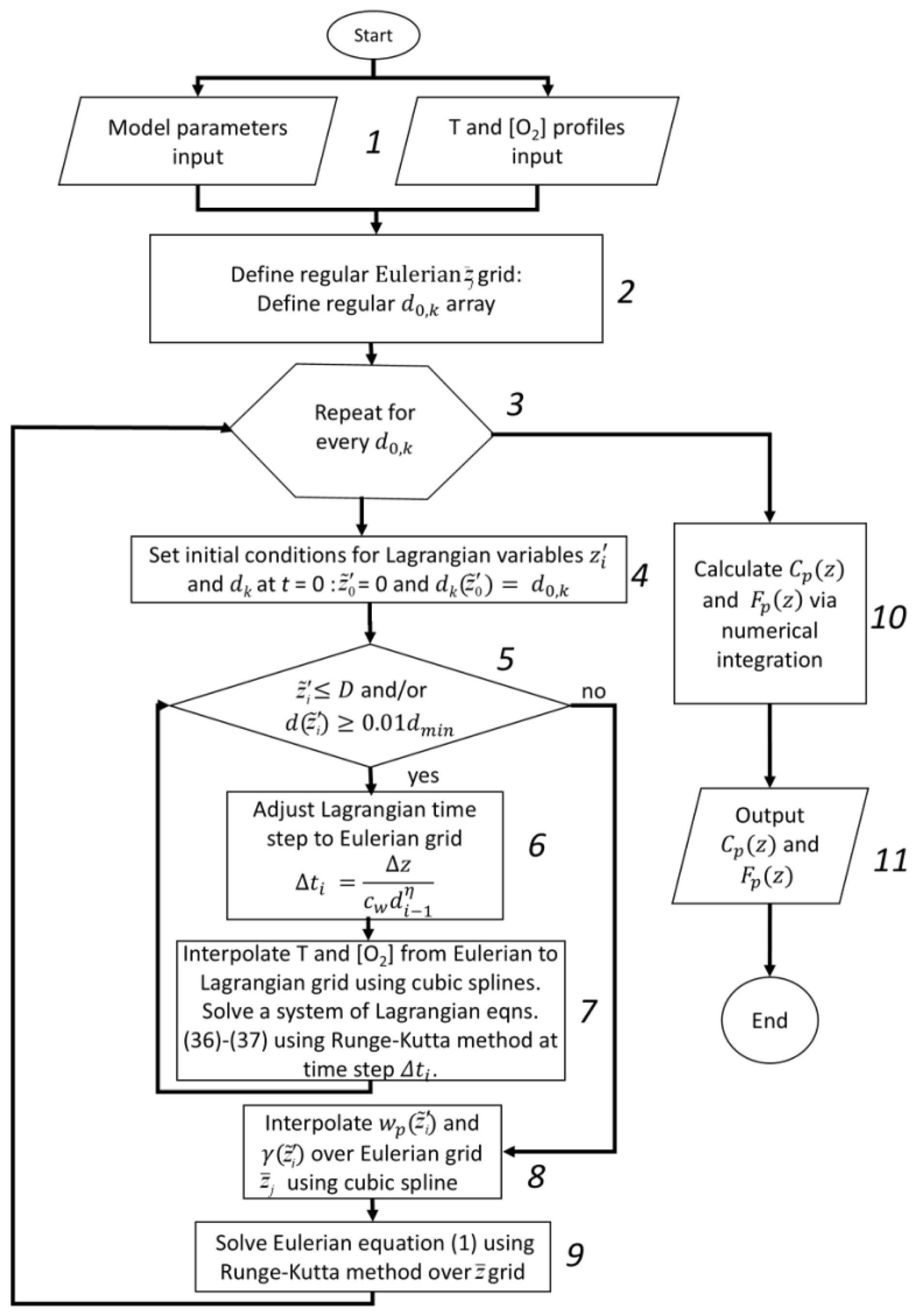
Figure 3 Eulerian–Lagrangian method flow chart for equations of sinking particulate organic matter.

The procedure for determining the profiles of C_p(z^′) and F_p(z^′) is presented in Fig. 3. It includes 11 steps.

• Step 1. The model parameters and temperature and oxygen concentration profiles are read from the input files.

• Step 2. A regular Eulerian grid ${\stackrel{\mathrm{‾}}{z}}^{\prime }$ is established from 0 to the ocean depth D with n_z equal intervals Δz with levels ${\stackrel{\mathrm{‾}}{z}}^{\prime }=j\cdot \mathrm{\Delta }z$, where $j=(\mathrm{0},n_z)$. The particle size spectrum at the lower boundary of the euphotic layer is divided into n_d equal intervals of size Δd in the range from d_min to d_max. For every particle size d_0,k, $k=(\mathrm{0},n_d)$.

• Step 3. Steps 4–9 are performed for every d_0,k, where $k=(\mathrm{0},n_d)$. Then, Step 10 is performed.

• Step 4. The initial conditions are set for the Lagrangian particle depth ${\stackrel{\mathrm{̃}}{z_k}}^{\prime }\left(t_i\right)$ and size $d=d_{\mathrm{0},k}$ equations at t_i=0.

• Step 5. If the Lagrangian particle depth ${\stackrel{\mathrm{̃}}{z_k}}^{\prime }\left(t_i\right)$ is equal to or greater than the ocean depth D or the particle diameter at this depth level $d=d_{\mathrm{0},k}$ is equal to or less than 1 % of the minimum diameter d_min, Step 8 is performed; otherwise, Step 6 is performed.

• Step 6. The timescale is divided into intervals Δt_i, $i=(\mathrm{0},n_t)$ over which Eqs. (36)–(37) are integrated. To align the resulting ${\stackrel{\mathrm{̃}}{z_k}}^{\prime }\left(t_i\right)$ and regular depth grid ${\stackrel{\mathrm{‾}}{z}}^{\prime }$, the ith timestep duration is calculated as $\mathrm{\Delta }{t}_{i,k}=\mathrm{\Delta }z/\left(c_w{d}_{i,k}^{\mathit{\eta }}\right)$.

• Step 7. The Lagrangian formulation with respect to time t is used to solve the system of Eqs. (36)–(37) via the Runge–Kutta method of the 4th order. Cubic spline interpolation is used to calculate the temperature and oxygen concentration at ${\stackrel{\mathrm{̃}}{z_k}}^{\prime }\left(t_i\right)$.

• Step 8. The $w_{\mathrm{p}}\left({\stackrel{\mathrm{̃}}{z_k}}^{\prime }\right(t_{i+\mathrm{1}}\left)\right)$ and $\mathit{\gamma }\left({\stackrel{\mathrm{̃}}{z_k}}^{\prime }\right(t_{i+\mathrm{1}}\left)\right)$ profiles on the Lagrangian grid are interpolated via a cubic spline over the Eulerian grid ${\stackrel{\mathrm{‾}}{z}}^{\prime }$.

• Step 9. $C_{\mathrm{p},d}\left({\stackrel{\mathrm{‾}}{z}}^{\prime }\right)$ is calculated by solving the Euler Eq. (1) via the Runge–Kutta method over the regular grid ${\stackrel{\mathrm{‾}}{z}}^{\prime }$. Then, Step 3 is performed.

• Step 10. The total POM concentration $C_{\mathrm{p}}\left({\stackrel{\mathrm{‾}}{z}}^{\prime }\right)$ and POM flux $F_{\mathrm{p}}\left({\stackrel{\mathrm{‾}}{z}}^{\prime }\right)$ are obtained via numerical integration of $C_{\mathrm{p},d}\left({\stackrel{\mathrm{‾}}{z}}^{\prime }\right)$ and $w_{\mathrm{p}}\left({\stackrel{\mathrm{‾}}{z}}^{\prime }\right))$ by using the composite Simpson's $\mathrm{1}/\mathrm{3}$ rule.

• Step 11. The model outputs the total POM concentration $C_{\mathrm{p}}\left({\stackrel{\mathrm{‾}}{z}}^{\prime }\right)$ and POM flux $F_{\mathrm{p}}\left({\stackrel{\mathrm{‾}}{z}}^{\prime }\right)$.

The code for the proposed algorithm, along with the data used in this study, is archived on Zenodo (Kovalets et al., 2025a, b).

4.2 Numerical model setup

Simulations were carried out for a water column with a depth of D=5000 m and Δz=1 m. We calculated the vertical profiles of the POM concentration C_p and flux F_p using AID and ADD models for the degradation rate. The remaining model parameters, with the exception of η, were adopted from Table 1. The profiles of C_p and F_p were calculated via the above algorithm with η=1.17 for comparison with the analytical solutions with the AID and ADD parameters from Table 1. As shown in Fig. 1, the numerical and analytical profiles coincide.

The calculation results were compared with the available measurement data for C_p and F_p for the latitude bands of 20–30° N in the Atlantic and Pacific Oceans and 50–60° S in the Southern Ocean. These calculations aimed to assess the relative effects of the vertical distributions of temperature and oxygen in the Atlantic, Pacific and Southern Oceans on the profiles of C_p and F_p. For the Atlantic Ocean, the C_p and F_p data are compiled in (Aumont et al., 2017) and (Lutz et al., 2002). For the Pacific Ocean, these values are presented in (Martin et al., 1987) and (Druffel et al., 1992). The Southern Ocean data for the Pacific and Atlantic sectors are presented in (Aumont et al., 2017) and (Lutz et al., 2002). The calculations required for averaging over the region and time profiles of T and [O₂] were performed with the measurement data from (Boyer et al. , 2018). These averaged profiles are shown in Fig. S1. Notably, there is great uncertainty not only in the choice of model parameter values but also in the parameterization of the processes. This is explained by both an insufficient understanding of the physical and biogeochemical processes and the lack of a sufficient number of measurements in the deep layers of the ocean. In particular, the observation results (Cael et al., 2021) show large deviations in the parameters of the sinking velocity–particle size relationship (Eq. 4). In recent models, the parameter η has varied from 0.26 (Alcolombri et al., 2021) to 2 (Omand et al., 2020). Therefore, in the simulations, we compared the effects of η on the C_p and F_p profiles for two values: η=1.17 (Smayda, 1970) and η=0.63 (Cael et al., 2021).

5 Modelling results

5.1 Comparison of simulations with measurements

Figures 4–6 show the profiles of C_p and F_p normalized to C_p(z_eu) and F_p(z_eu). They were calculated using the numerical algorithm described in Sect. 4.1. These profiles are compared with normalized measurements in the subtropical zones of the Atlantic (Fig. 4) and Pacific (Fig. 5) Oceans and in the Atlantic and Pacific sectors of the Southern Ocean (Fig. 6) to consider the effects of temperature and oxygen concentration on POM. When the modelling results are compared with the measurement data, the significant scatter of the measurement data presented in Figs. 4–6 must be noted. This scatter is due both to the difficulties of measuring the concentration and flux of particles and to regional differences in the influx of particles and in the surrounding ocean.

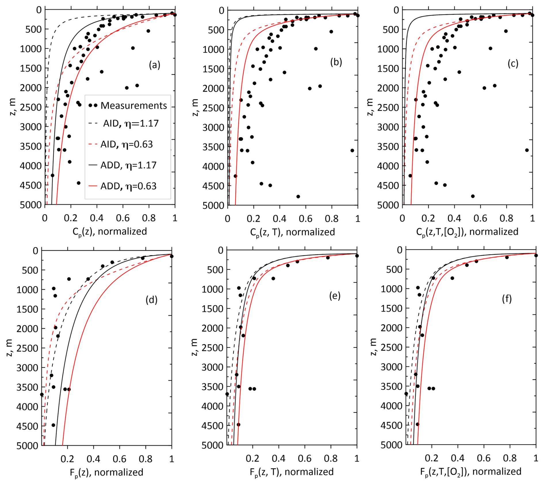
Figure 4 Normalized total POM concentration C_p (a–c) and total POM flux F_p (d–f) versus measurement data in the Atlantic Ocean at 20–30° N (Aumont et al., 2017; Lutz et al., 2002). Three columns of panels correspond to the model without dependency of temperature and oxygen (panels a and d), additional temperature dependence (panels b and e), and both additional dependencies (panels c and f).

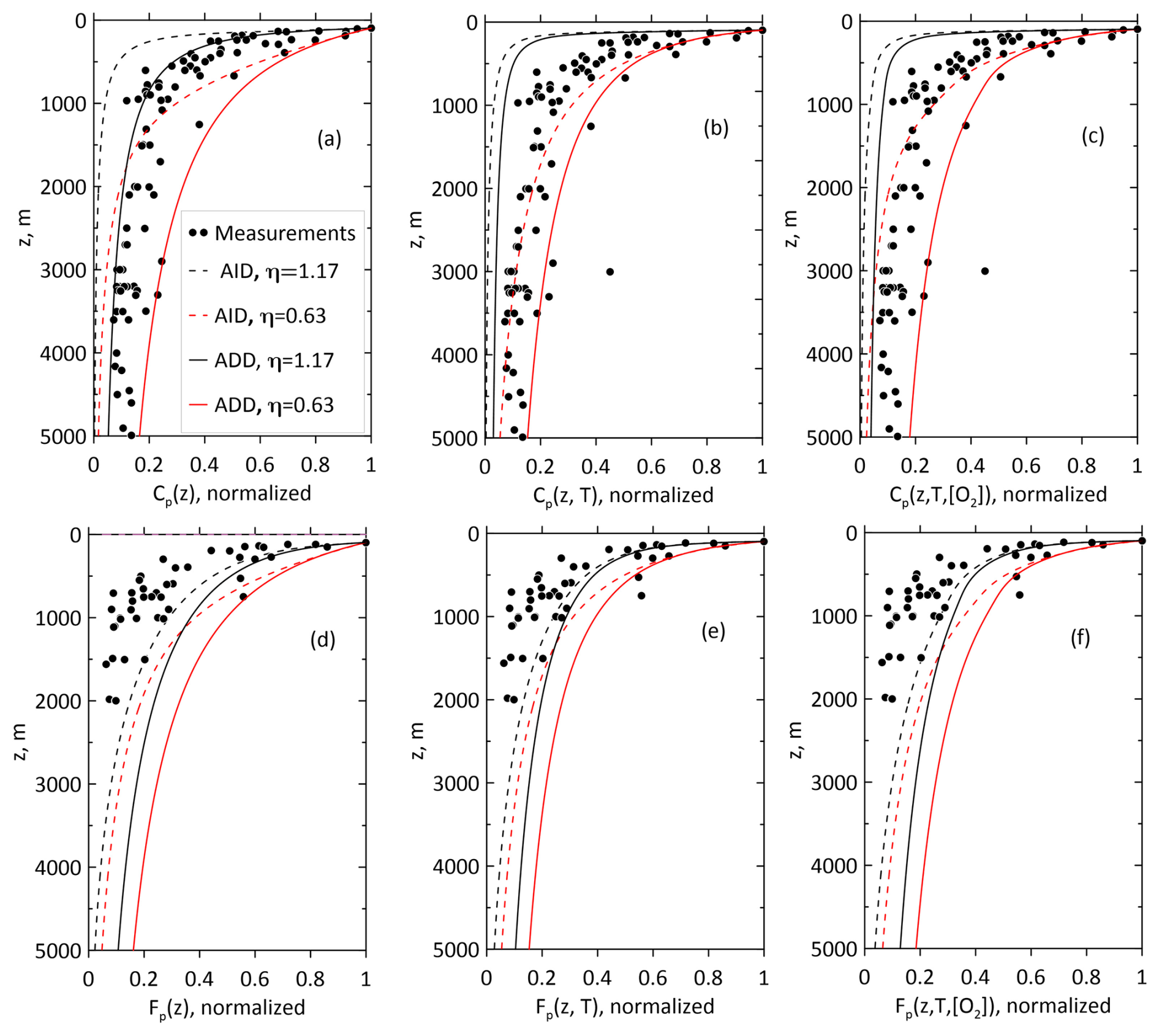
Figure 5 Normalized total POM concentration C_p (a–c) and total POM flux F_p (d–f) versus measurement data in the Pacific Ocean at 20–30° N (Martin et al., 1987; Druffel et al., 1992). Three columns of panels correspond to the model without dependency of temperature and oxygen (panels a and d), additional temperature dependence (panels b and e), and both additional dependencies (panels c and f).

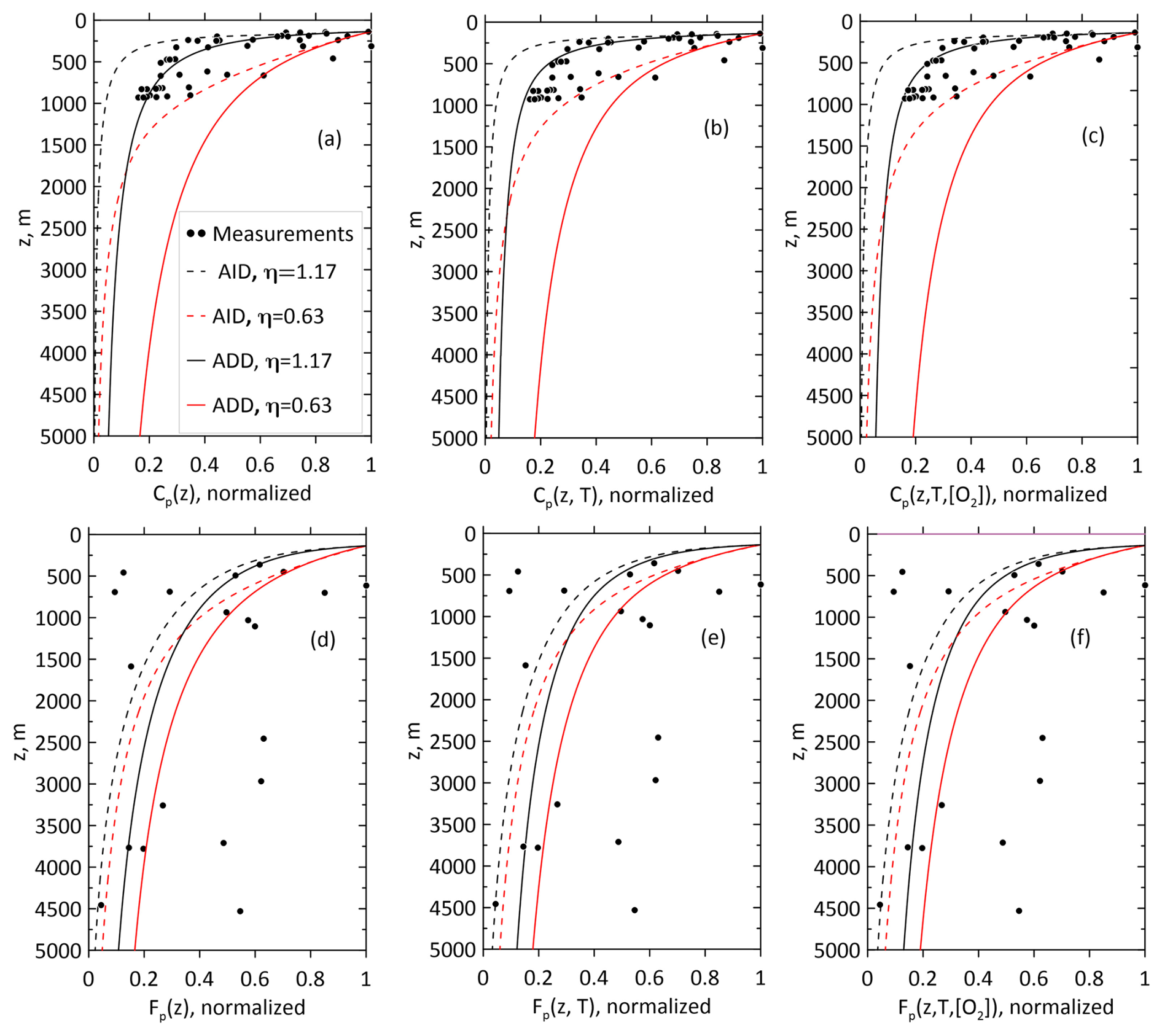
Figure 6 Normalized total POM concentration C_p (a–c) and total POM flux F_p (d–f) versus measurement data in the Southern Ocean at 50–60° N (Aumont et al., 2017; Lutz et al., 2002). Three columns of panels correspond to the model without dependency of temperature and oxygen (panels a and d), additional temperature dependence (panels b and e), and both additional dependencies (panels c and f).

The C_p and F_p profiles in Figs. 4–6 were obtained for three variants of the degradation model. In the first variant (plots a and d), C_p and F_p do not depend on the temperature or oxygen concentration. In the second variant (plots b and e), they do not depend on the oxygen concentration, and in the third variant (c and f), they depend on the temperature and oxygen concentration. The first variant is described by analytical solutions for the AID and ADD models. The features of these solutions are discussed in Sect. 3.3. The profiles of C_p and F_p are sensitive to the value of η. The solutions with η=0.63 decay more slowly than those with η=1.17 do, as shown by the analytic solutions in Figs. 4a, 4d, 5a, 5d, 6a, and 6d.

The use of the AID model led to a more rapid decay of C_p with depth than was observed in all the ocean profiles. Moreover, the application of the ADD model resulted in smoother profiles in all oceans; however, the AID and ADD profiles are qualitatively close. As shown in Figs. 4b, 4e, 5b, 5e, 6b, and 6e, the dependence of the degradation rate on temperature significantly affected the C_p and F_p profiles; namely, it enhanced the degradation of sinking particles in the upper layers of the ocean and suppressed it in the deep layers of the ocean. The influence of the oxygen concentration in all the cases considered (Figs. 4c, 4f, 5c, 5f, 6c, and 6f) was less significant than that of the distribution of temperature with depth. Overall, including temperature and concentration dependence in the degradation rate relationship improved the agreement with ocean measurements. The normalized mean bias errors (MBEs) when considering the dependence of the degradation rate on temperature and oxygen concentration (third variant) decreased from 9 % to −3 % compared to those of the first variant, when this dependence was not considered. For the third variant, the root mean square deviation (RMSD) decreased by half compared with that of the first variant.

Notably, both the AID and ADD models somewhat underestimated F_p when the dependence on temperature was considered. As shown in Figs. 4–6, the use of the AID model led to a more rapid decay of C_p with depth than was observed in all ocean profiles. Moreover, the decay of F_p with depth occurred more slowly in most of the measured profiles. The use of the ADD model (Figs. 4–6) resulted in smoother profiles; however, qualitatively, the AID and ADD profiles are similar. Notably, profiles C_p and F_p in Fig. 3c, 3f and 4c, 4f are quite close despite the differences between the temperature and oxygen concentration profiles in the 20–30° N band of the Atlantic and Pacific Oceans (Fig. S1a–b). These profiles in the colder, oxygen-saturated waters of the Southern Ocean (Fig. S1c) attenuate more slowly with depth.

5.2 Sensitivity study

As shown in Figs. 4–6, the model output was sensitive to parameters with high uncertainty, such as η. Therefore, a sensitivity study was carried out for the model parameters in Table S1. We used the one-at-a-time method to quantify the effect of variation in a given parameter on the model output while all other parameters were kept at their initial values (Hamby, 1994; Lenhart et al., 2002; Soares and Calijuri , 2021). The effects of variations in these parameters were estimated for the particle transfer efficiency (TE). TE₁₀₀₀ is defined as the ratio of the POM flux at the lower level of the euphotic layer z_eu to the flux at the lower boundary of the mesopelagic layer z=1000, and TE₅₀₀₀ is defined as the ratio of the POM flux at the lower level of the euphotic layer to the flux in the bottom layer at z=5000 m. The ranges for the parameters were defined for a constant ratio r>1. The minimum parameter value p_min was set to be proportional to the reference value p_ref with a ratio value of $\mathrm{1}/r$, whereas the maximum value p_max was set to be proportional to the reference value p_ref with a ratio value of r. For the parameters in Table S1, the value of r was chosen to be the same (r=1.25), which satisfies the ranges of all the parameters.

The model output sensitivity was estimated using a sensitivity index (SI) defined as

$$\begin{array}{}\text{(38)}& \mathrm{SI}={\displaystyle \frac{\mathrm{TE}\left(p_{\max }\right)-\mathrm{TE}(p_{\min )}}{\mathrm{TE}\left(p_{\mathrm{ref}}\right)}},\end{array}$$

where TE(p_max), TE(p_min) and TE(p_ref) are the simulation results for the maximal p_max, minimal p_min, and reference p_ref parameter values, respectively. Calculations of SI were carried out for the Pacific Ocean for the AID and ADD models with the reference, maximal and minimal values of the parameters from Table S2.

The sensitivity index SI(TE₁₀₀₀) is shown in Fig. 7a for the parameters of the AID model. As shown in the figure, SI(TE₁₀₀₀) was most sensitive to the exponent ζ in the power law dependence of the particle mass on the particle size (Eq. 3) and to the exponent ϵ in the power law dependence of the particle size distribution at the lower boundary of the euphotic layer (Eq. 16). The sign of the index indicates whether the model reacted codirectionally to the input parameter change, i.e., whether the parameter increase/decrease corresponded to an increase/decrease in the model output parameter. The nature of the dependence of SI(TE₁₀₀₀) on ζ and ϵ was different. An increase in ζ resulted in an increase in TE₁₀₀₀, i.e., an increase in the mass of a particle increased the transfer efficiency. Moreover, an increase in ϵ resulted in a decrease in TE₁₀₀₀, i.e., an increase in the slope of the spectral particle size distribution led to a decrease in the transfer efficiency. The dependence of SI(TE₁₀₀₀) on T_ref and K_O was weak (SI ≪1), whereas the dependence on γ₀, η and Q₁₀ was moderate. The sensitivity index SI(TE₅₀₀₀) for the parameters of the AID model is shown in Fig. 7b. As shown in the figure, it is qualitatively similar to that in Fig. 7a. Four parameters (${\mathit{\gamma }}_{\mathrm{0}},\mathit{\zeta },\mathit{\eta },$ and ϵ) showed strong sensitivity.

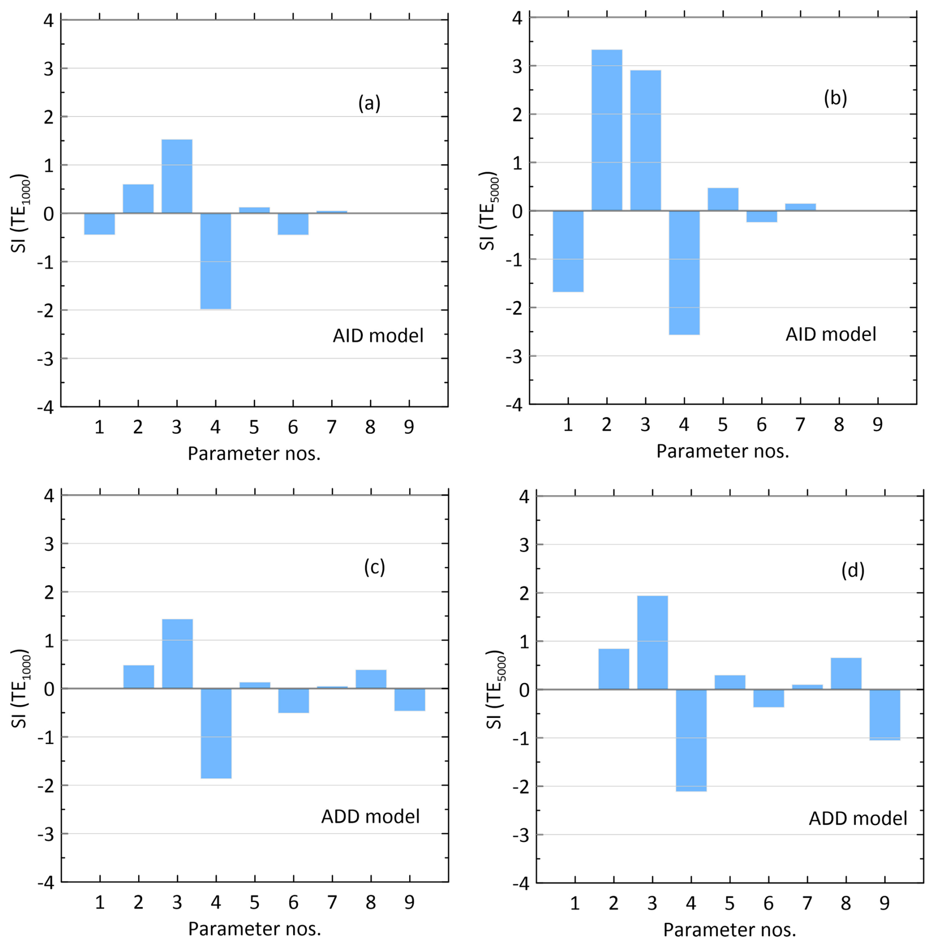
Figure 7 Sensitivity indexes SI(TE₁₀₀₀) and SI(TE₅₀₀₀) for parameters given in Table S2. Panels (a) and (b) correspond to the AID model, whereas panels (c) and (d) correspond to the ADD model.

The sensitivity index SI(TE₁₀₀₀) values for the parameters of the ADD model are shown in Fig. 7c. Similar to the results in Fig. 7a, TE₁₀₀₀ was most sensitive to ζ and ϵ; however, the amplitudes of SI(TE₁₀₀₀) were less than those for AID model. The sensitivity of the ADD model parameters (α and β) was moderate. The sensitivity index SI(TE₅₀₀₀) values for the parameters of the ADD model are shown in Fig. 7d. Similar to SI(TE₁₀₀₀) for this model, the magnitudes of the SI(TE₅₀₀₀) values were greater than the magnitudes of the SI(TE₅₀₀₀) values. Additional details on the sensitivity study are presented in the Supplement.

6 Discussion and conclusions

In this work, we considered a simple Eulerian–Lagrangian approach for solving equations that describe the gravitational sinking of organic particles under the effects of the sizes and ages of the particles, temperature and oxygen concentration on their dynamics and degradation processes. In contrast to other approaches, our approach does not solve particle size spectrum equations (e.g., DeVries et al., 2014) explicitly or introduce power-law particle size distribution assumptions below the euphotic layer (e.g., Kriest and Evans , 1999; Maerz et al., 2020). Note that the particular form of size spectrum dependence N(d₀) may differ from the power law (Eq. 15). Unlike (Omand et al., 2020), we do not assume a priori the constancy of the particle flux in depth in steady state. Instead, solutions are found for the Euler equation for the concentration of particles of a given size and the Lagrange equations for a sinking organic particle under the influence of microbiological degradation. In the stationary case, the problem is reduced to solving a system of ordinary differential equations of the first order, in contrast to (DeVries et al., 2014), where the solution of the hyperbolic equation of the first order for the particle distribution is found. In addition, the total concentration and flux of the POM are found by summation over the particle distribution at $z^{\prime }=\mathrm{0}$, whereas in (DeVries et al., 2014) the summation is carried out over all depths. As shown in Table 3 from the review (Burd, 2024), in CMIP6 Eulerian biogeochemical models, the sinking velocity is either assumed to be constant or it increases linearly with depth. Our hybrid approach considers the interaction between the sinking and degradation processes of POM particles in Lagrangian variables and POM concentration in the Eulerian coordinate system, making particle transport models compatible with large-scale Eulerian biogeochemical models. It also provides an opportunity to solve the non-stationary problem in the future using Eq. (1) complemented by the time derivative of C_p,d and necessary parameterizations of the POM sinking processes.

Novel analytical solutions of the system of the one-dimensional Eulerian equation for the POM concentration and Lagrangian equations for the particle mass and depth were obtained for constant and age-dependent degradation rates. The feedback between the degradation rate and sinking velocity results in significant changes in the POM concentration and flux profiles. In the case of a constant γ₀ (AID model), the vertical distribution of the concentration C_p,d for a single fraction of the POM size d₀ at z_eu is limited by a finite layer, unlike the exponential profile of the particle concentration that corresponds to a constant sinking velocity. Particles in such a finite layer sink at a linearly decreasing velocity. Moreover, the distributions of the total particle concentration C_p and flux F_p approach exponential trends with depth for increasing d₀ fractions.

In contrast to those for the AID model, the vertical distributions of the concentration and vertical velocity decay asymptotically with depth for the ADD model. The rates of degradation of the Eulerian variables decay with depth; however, the corresponding exponent depends not only on the parameter β, as in the models with constant sinking velocity (Cael et al., 2021), but also on the parameters that characterize the vertical velocity η and porosity ζ of the particles. With the baseline parameters, the vertical distribution of C_p is close to the power distribution with an exponent of approximately 1, whereas the distribution with the depth of the total particle flow F_p deviates significantly from the power law dependence (“Martin's law”). Direct comparison with other models is difficult owing to differences in the parameterizations of processes, with the exception of the model (DeVries et al., 2014) for which the solutions of the equations for the particle spectrum and concentration are established (Appendix A).

A new Eulerian–Lagrangian numerical approach for solving the problem in general cases was presented. The algorithm includes time steps for Lagrangian variables (sinking velocity and particle mass) and Eulerian depth steps for the concentration of particles of size d. This enables the inclusion of different parameterizations of interacting degradation and sinking processes (e.g., DeVries et al., 2014; Cram et al., 2018; Omand et al., 2020; Alcolombri et al., 2021). However, in this study, we limited ourselves to the case where the degradation rate depends on the age of the organic particle, the temperature of the sea water and the concentration of oxygen. Notably, the developed numerical algorithm is suitable for arbitrary dependencies of mass and sinking velocity on the particle diameter. The proposed numerical method was tested on the obtained analytical solutions.

The calculation results were compared with the available measurement data for the POM concentrations and POM fluxes for the latitude bands of 20–30° N in the Atlantic and Pacific Oceans and 50–60° S in the Southern Ocean. The dependence of the degradation rate on temperature affects the profiles of the total particle concentration and flux significantly; it enhances the degradation of sinking particles in the upper layers of the ocean and suppresses it in the deep layers of the ocean. Overall, including temperature and concentration dependence in the degradation rate relationship improves the agreement with ocean measurements. In particular, the normalized MBEs when considering the dependence of the degradation rate on temperature and oxygen concentration were reduced from 9 % to −3 % compared with cases in which this dependence was not taken into account. Similarly, on average, the RMSD decreased by half when temperature stratification was considered.

The discrepancies between the model predictions and observations were caused by incomplete descriptions of processes and uncertainties in model parameters, as well as variability in the measured POM concentration and flux profiles owing to vertical and horizontal variability in the ocean fields. We used the one-at-a-time method to quantify the effect of the variation of one parameter from the set (${\mathit{\gamma }}_{\mathrm{0}},\mathit{\eta },\mathit{\zeta },\mathit{ϵ},T_{\mathrm{ref}},Q_{\mathrm{10}},K_{\mathrm{0}},\mathit{\alpha },\mathit{\beta }$) on the model output, with all other parameters kept at their initial values. The effects of variations in these parameters on the particle transfer efficiency TE were estimated as the ratio of the POM flux at z_eu to the value at a depth of 1000 or 5000 m. The model output sensitivity was estimated via the sensitivity index SI (Eq. 38). Calculations for the Pacific Ocean revealed that TE₁₀₀₀ and TE₅₀₀₀ are most sensitive to the parameters ζ and ϵ, respectively, for both models. Therefore, these parameters should be primarily calibrated and optimized. Therefore, it was important to assess the sensitivity of the calculations to the values of the model parameters.

Notably, to obtain analytical solutions and demonstrate the numerical Eulerian–Lagrangian approach, significant simplifications were made in the description of the particle dynamics. In particular, the particle sinking velocity was described in the Stokes approximation. The aggregation and fragmentation of particles, mineral ballasting, ocean density stratification, and temporal changes in particle fluxes were not considered. While some simplifications can be eliminated by using a numerical approach, others require significant generalization. This applies particularly to the description of particle ballasting mechanisms. On the one hand, ballast affects the sinking of particles, but on the other hand, ballast minerals can protect organic matter from degradation (Cram et al., 2018). The processes of fragmentation and consumption of sinking particles, which are important in the upper mesopelagic layer, are poorly understood (Burd, 2024). Comparison of calculation results for different parameter values (e.g. η) did not reveal the advantage of one parameter value for both C_p and F_p, which may be due to the incompleteness of the description of the processes of the simplified model used. Therefore, for the effective application of the proposed approach in biogeochemical models, a parameterization of the main process controls of the biological carbon pump mechanism based on data from natural and laboratory measurements is necessary.

Appendix A: Derivation of the spectral solution for the size distribution (DeVries et al., 2014)

Here, we show that the analytical solution (14) for C_p,d is equivalent to the solution (8) from (DeVries et al., 2014) of the spectral equation for the particle size distribution. To find the particle size distribution at z^′, we first rearrange Eq. (12) to obtain the relationship between d₀ and d at depth z^′:

$$\begin{array}{}\text{(A1)}& d_{\mathrm{0}}=d{\left(\mathrm{1}+{\displaystyle \frac{\mathit{\eta }{\mathit{\gamma }}_{\mathrm{0}}}{\mathit{\zeta }{c}_w{d}^{\mathit{\eta }}}}{z}^{\prime }\right)}^{\mathrm{1}/\mathit{\eta }}.\end{array}$$

The size distribution N(d,z) [m⁻⁴] is related to C_p,d and m_d as

$$\begin{array}{}\text{(A2)}& C_{\mathrm{p},d}\mathrm{\Delta }{d}_{\mathrm{0}}=N{m}_d\mathrm{\Delta }d,\end{array}$$

where Δd is a small increment. Combining Eqs. (14), (3), (12), and (A2) yields

$$\begin{array}{}\text{(A3)}& \begin{array}{rl}N(d,z^{\prime })& ={\displaystyle \frac{C_{\mathrm{p},d}\mathrm{\Delta }{d}_{\mathrm{0}}}{m_d\mathrm{\Delta }d}}\\ & ={\displaystyle \frac{\mathrm{\Delta }{d}_{\mathrm{0}}}{\mathrm{\Delta }d}}{M}_{\mathrm{0}}{d}_{\mathrm{0}}^{-\mathit{ϵ}}{\left(\mathrm{1}+{\displaystyle \frac{\mathit{\eta }{\mathit{\gamma }}_{\mathrm{0}}}{\mathit{\zeta }{c}_w{d}^{\mathit{\eta }}}}{z}^{\prime }\right)}^{\frac{\mathit{\eta }-\mathit{ϵ}}{\mathit{\eta }}}.\end{array}\end{array}$$

At the limit of Δd→0, we obtain

$$\begin{array}{}\text{(A4)}& \underset{\mathrm{\Delta }d\to \mathrm{0}}{lim}{\displaystyle \frac{\mathrm{\Delta }{d}_{\mathrm{0}}}{\mathrm{\Delta }d}}={\displaystyle \frac{d}{dd}}{d}_{\mathrm{0}}={\left(\mathrm{1}+{\displaystyle \frac{\mathit{\eta }{\mathit{\gamma }}_{\mathrm{0}}}{\mathit{\zeta }{c}_w{d}^{\mathit{\eta }}}}{z}^{\prime }\right)}^{\frac{\mathrm{1}-\mathit{\eta }}{\mathit{\eta }}}.\end{array}$$

Then, Eq. (A3) can be written as

$$\begin{array}{}\text{(A5)}& N(d,z^{\prime })=M_{\mathrm{0}}{d}^{-\mathit{ϵ}}{\left(\mathrm{1}+{\displaystyle \frac{\mathit{\eta }{\mathit{\gamma }}_{\mathrm{0}}}{\mathit{\zeta }{c}_w{d}^{\mathit{\eta }}}}{z}^{\prime }\right)}^{\frac{\mathrm{1}-\mathit{ϵ}}{\mathit{\eta }}}.\end{array}$$

This solution for N coincides with that obtained by DeVries et al. (2014).