Copernicus Atmosphere Monitoring Service – Regional Air Quality Production System v1.0

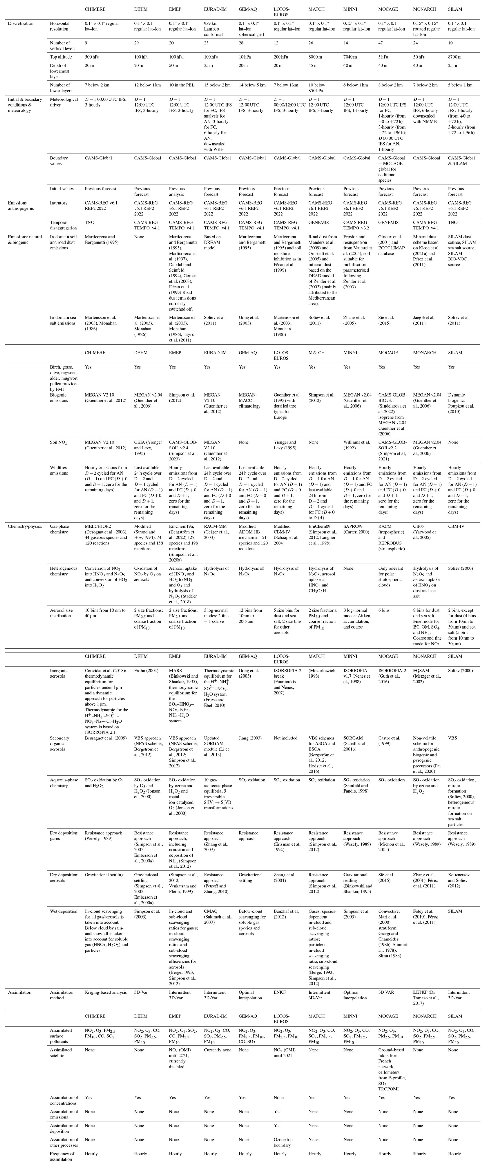
The Copernicus Atmosphere Monitoring Service (CAMS) delivers a wide range of free and open products in relation to atmospheric composition at global and regional scales. The CAMS Regional Service produces daily forecasts, analyses, and reanalyses of air quality in Europe. This service relies on a distributed modelling production by 11 teams in 10 European countries: CHIMERE (France), DEHM (Denmark), EMEP (Norway), EURAD-IM (Germany), GEM-AQ (Poland), LOTOS-EUROS (the Netherlands), MATCH (Sweden), MINNI (Italy), MOCAGE (France), MONARCH (Spain), and SILAM (Finland). The project management and coordination of the service is conducted by a Centralised Regional Production Unit. Every day, each model produces 24 h analyses for the previous day and 97 h forecasts for 19 chemical species over a spatial domain at 0.1 × 0.1° resolution (approximately 10 km × 10 km), with 420 points in latitude and 700 in longitude and 10 vertical levels. Six pollen species are also delivered for the surface forecasts. The 11 individual models are then combined into an ENSEMBLE median. In total, more than 82 billion data points are made available for public use on a daily basis.

The design of the system follows clear technical requirements in terms of consistency in the model setup and forcing fields (meteorology, surface anthropogenic emission fluxes, and chemical boundary conditions). But it also benefits from a diversity in the description of atmospheric processes through the design of the 11 European chemistry-transport models (CTMs) involved.

The present article aims to provide a comprehensive technical documentation, both for the setup and for the diversity of CTMs involved in the service. We also include an overview of the main output products, their public dissemination, and the related evaluation and quality control strategy.

1 Introduction

The Copernicus Atmosphere Monitoring Service (CAMS, https://atmosphere.copernicus.eu/, last access: 8 September 2025) is the core global and regional atmospheric environmental service operated by the European Centre for Medium-Range Weather Forecast (ECMWF) within the European Union Copernicus Earth Observation Programme. It provides a wide range of free, open, and quality-assured products in relation to global and regional air quality, inventory-based emissions, observation-based surface fluxes of greenhouse gases and from biomass burning, solar energy, ozone and UV radiation, and climate forcings (Peuch et al., 2022).

We focus here on the Regional Production Service (https://atmosphere.copernicus.eu/european-air-quality-forecast-plots/, last access: 8 September 2025), which provides daily 4 d forecasts of the main air quality species and analyses of the day before, as well as posterior reanalyses using the latest observation datasets available for assimilation. Today it constitutes the reference air quality forecasting system at a European scale by building upon a distributed production of 11 chemistry-transport models operated in 10 European countries, with a Centralised Regional Production Unit to ensure a consistent implementation. Such a comprehensive air quality forecasting system operated at a continental scale has no equivalent in the world.

Air quality monitoring and forecasting constitute an essential activity to improve the knowledge of atmospheric composition and air pollution patterns and identify short and long-term mitigation strategies. In European legislation, the directive (EC, 2008) on ambient air quality and cleaner air for Europe of the European Parliament and of the European Council defines limit and target values for regulatory ambient air concentrations and improvement of ambient air quality to avoid, prevent, or reduce harmful effects on human health and the environment. To this end, it sets out the methodological requirements for the assessment of ambient air quality in Member States, which are based on the implementation of adequate monitoring systems, typically relying on reference and standardised instruments operated at air quality monitoring stations, whose data are reported to the Air Quality e-reporting database maintained by the European Environment Agency (which subsequently makes the data publicly available). A revision of the Ambient Air Quality Directive was adopted by the European Council in October 2024; the revision includes, amongst other features, a stronger emphasis on the use of air quality models as well as an explicit reference to the Copernicus Atmosphere Monitoring Service as a trusted source of information products and supplementary tools to support reporting activities in relation to forecasting and management of air pollution episodes.

Modelling provides complementary information on ambient air quality. Fitness for forecasting purposes of air quality modelling has been widely documented (Zhang et al., 2012b, a), but air quality models are also essential to produce exposure maps through data assimilation or data fusion. In such processes, the prior modelled estimates of surface air concentrations of the main air pollutants are combined with in situ or remote sensing observations to produce improved mapping of air pollution, typically for use in health impact assessment or epidemiological studies (Shaddick et al., 2020). Air quality modelling and reanalyses are also typically used to anticipate the effectiveness of policy mitigation strategies ex ante and assess them ex post. The projections and hindcasts performed in the framework of the Convention on Long Range Transboundary Air Pollution (CLRTAP) of the United Nations Economic Commission for Europe Geneva Air Convention and its Gothenburg Protocol constitute a good example of atmospheric modelling activities in support of policy decisions at a European scale (Maas and Grennfelt, 2016).

Whereas several European countries or selected metropolitan areas operate their own air quality modelling system, there is also a need to produce air quality forecasts and analyses over the whole European continent: to provide background data for those local systems (chemical boundary conditions), for the areas not covered by any national system or just as complementary information. The Copernicus Atmosphere Monitoring Service has played that role since 2015. It builds upon the earlier research and development phases initiated since 2005 through European collaborative research and innovation projects: GEMS (Hollingsworth, 2008) and MACC, MACC-II, and MACC-III (Marécal et al., 2015; Peuch et al., 2014).

The unique setup of the system allows it to reach an unprecedented level of quality and robustness by relying on a set of stringent common requirements combined with a large variety of chemistry-transport models (CTMs). Since 2022, an ensemble of 11 CTMs have been used: CHIMERE (INERIS, France), DEHM (Aarhus Univ., Denmark), EMEP (Met Norway), EURAD-IM (Forschungszentrum Jülich, Germany), GEM-AQ (IEP-NRI, Poland), LOTOS-EUROS (TNO and KNMI, the Netherlands), MATCH (SMHI, Sweden), MINNI (ENEA, Italy), MOCAGE (Météo-France, France), MONARCH (BSC, Spain), and SILAM (FMI, Finland). Using an ensemble of CTMs allows the risk of failure in the daily operational production to be minimised and the skill of the forecast to be increased at the same time (Galmarini et al., 2013). But consistency in the implementation is key to ensure the continuous improvement of the system, hence the crucial role of the CAMS Regional Central Production Unit led by Météo-France and INERIS.

Every day, each model delivers 24 h analyses and 97 h forecast for 19 chemical species over a spatial domain at 0.1 × 0.1° resolution (approximately 10 km × 10 km), with 420 points in latitude and 700 in longitude and 10 vertical levels. Additionally, surface forecasts of six pollen species are delivered. With the 11 individual models and one ENSEMBLE median, there is a total of almost 82 billion data points made available for public use every day.

The results of the CAMS Regional Service are made publicly available as quicklooks on the website (https://atmosphere.copernicus.eu/european-air-quality-forecast-plots, last access: 8 September 2025), and the numerical outputs are disseminated on the Copernicus Atmosphere Data Store (ADS) (https://ads.atmosphere.copernicus.eu, last access: 8 September 2025). The typical use of the forecasts is as background information used by national and local air quality agencies, in addition to their knowledge about specific local air pollution sources. This can be done either qualitatively by the consultation of available online viewers or using the numerical data to feed downstream chemistry-transport, Gaussian, or machine-learning models. The use of reanalyses is rather for policy applications (for regulatory reporting obligations or to assess the impact policy interventions through trends analyses) or exposure assessment in health impact studies.

The aim of the present article is to provide a transparent and detailed documentation to serve as a reference for the user of CAMS Regional Air quality Products. It constitutes an update of the previous similar article devoted to the MACC regional forecast system (Marécal et al., 2015), whereas the system was still in research mode at the time and not fully operational. A focus on regional activities within the overall CAMS portfolio was also described in Peuch et al. (2022). The CAMS Regional Production System has evolved continuously over the past. In the present article, we provide a detailed description of the system as it stood in 2024. But since the near-real-time production of forecast and analysis remains available for public use with a 3-year retention time, and reanalysis data remain available for the period since the beginning of the production, we also provide some information about the major evolutions in the recent past.

The main characteristics of the centralised production system are introduced in Sect. 2. This section covers the overall production workflow but also the common features and requirements which apply to the distributed production of individual modelling teams such as the common external forcing data. Since the use of an ensemble of 11 different chemistry-transport models is an important specificity of the service, we devote a large part of the paper in Sect. 3 to summarise the formulation of each model and how they adapt specifically to the requirement of the CAMS Regional Production System. The post-processing and some elements regarding the evaluation and quality control or the main uses of the production are presented in Sect. 4. In the conclusion (Sect. 5), we refer to the short- and long-term development priorities to ensure the performance and sustainability of the system over the long term.

2 Centralised Regional Production Unit

2.1 Organisation of the production system

The CAMS Regional Production System relies on quite a unique ensemble of 11 individual models whose daily operation is distributed amongst 11 modelling centres in 10 European countries. The coordination is handled by the Central Regional Production Unit (CRPU), which is led by Météo-France, with the support of INERIS for model development matters and reanalysis production (Fig. 1).

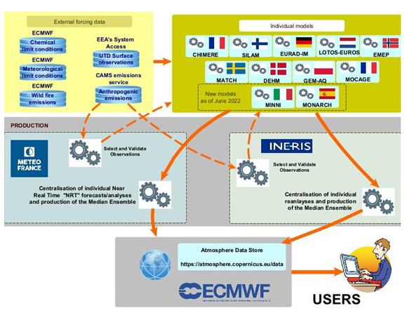
Figure 1 Schematic of the CAMS Regional Production workflow. Top left: external forcings (anthropogenic emissions, meteorology, boundary conditions) and in situ observations for assimilation and evaluation. Top right: 11 regional chemistry-transport models operated in 10 European countries. Middle: Meteo-France (for the near-real time) and INERIS (for the reanalysis) centralise the individual productions. Bottom: the results are disseminated to the Atmosphere Data Store.

The CRPU defines the design of the Regional Production System under the auspices of ECMWF. This includes setting the guidance and requirements for the implementation of individual models as well as continuous evolution in order to maintain the system within the state of the art. The CRPU is also in charge of contractual matters and relations with the providers of input data as well as the delivery of model results to the Atmosphere Data Store for public use (Sect. 4.3).

In earlier MACC phases and the first CAMS Regional project, only seven models were contributing to the distributed operational production: CHIMERE, EMEP, EURAD-IM, LOTOS-EUROS, MATCH, MOCAGE, and SILAM. As of October 2019, DEHM and GEM-AQ joined the operational system. As of June 2022, MINNI and MONARCH joined the production.

2.2 Modelling products

The CAMS Regional system includes both daily 4 d forecasts and several analysis products. All of them are provided from both 11 individual CTMs results and an ENSEMBLE product, which is constituted by the median of individual models at each grid point (see also Sect. 4 on post-processing).

Hourly near-real-time forecasts (NRT/FC) are released every day with a 4 d horizon (from 0 to 96 h forecasts). They rely on chemistry-transport outputs, some of which are initialised on the basis of the previous analysis (see details in Sect. 3). The ENSEMBLE NRT/FC fields are made available publicly each day at 08:00 UTC for forecast horizon 0 to 48 h (day 1 and day 2) and at 10:00 UTC for forecast horizon 49 to 96 h (day 3 and day 4). All the forecasts are initiated at 00:00 UTC; the differentiated timing for the 48 or 96 h lead time is only to account for longer production times.

The list of output species has been expanding gradually over the years. The choice of selected species accounts for user requests, especially with regards to downstream modelling needs (in the case where the CAMS Regional system is used as forcing boundary conditions for smaller-scale nested models), understanding air pollution episodes, and availability of observation data for evaluation and quality control (which is essentially focusing on PM₁₀, PM_2.5, NO₂, O₃, and pollens at present, but research-grade measurement of the EMEP Monitoring Programme or the ACTRIS European Research Infrastructure is considered to strengthen the quality control procedures).

As of April 2025, the list of species in the NRT/FC includes the following gases: ozone (O₃), nitrogen oxide (NO), nitrogen dioxide (NO₂), carbon monoxide (CO), sulfur dioxide (SO₂), glyoxal (CHOCHO), formaldehyde (HCHO), ammonia (NH₃), total non-methane volatile organic compounds (NMVOCs, defined as the sum of the mass of the carbon atoms of all the VOC species of the chemical scheme of the model, excluding the methane and PAN species, and expressed in unit µg m⁻³ of carbon atoms), and total peroxy acetyl nitrates (PANs). Particulate matter (PM) is included as PM_2.5 (smaller than 2.5 µm) and PM₁₀ (smaller than 10 µm). The following tracers in the PM_2.5 fraction are also provided: sulfate (SO${}_{\mathrm{4}}^{\mathrm{2}-}$), nitrate (NO${}_{\mathrm{3}}^{-}$), ammonium (NH${}_{\mathrm{4}}^{+}$), total secondary inorganic aerosols (SIAs), total elemental carbon (EC), EC fraction related to residential emissions, and total organic matter. In the PM₁₀ fraction, the tracers include desert dust, sea salt, and wildfires. In addition, six pollen species are included: birch, olive, grass, alder, mugwort, and ragweed.

Hourly near-real-time analysis (NRT/AN) is released each day by 12:00 UTC for the previous day. Here, each individual model is corrected to minimise error with observed air pollutant concentrations over Europe. For the latest reanalysis available on the ADS as of January 2024 (covering the year 2021), the list of species is for O₃, NO, NO₂, CO, NH₃, NMVOCs, PM₁₀, PM_2.5, PM₁₀ wildfires, PM₁₀ dust, EC total, EC residential, PAN, SIA, and SO₂. For earlier years, not all of these species are available, and in the future the list will continue expanding to catch up with the full species set in the daily forecast production. Note that observations are available for assimilation only for NO₂, O₃, PM₁₀, and PM_2.5. Individual components contributing to the total PM₁₀ or PM_2.5 mass are scaled according to the assimilation of total PM₁₀ or PM_2.5 measurements, and pollen species are not assimilated.

The daily analyses products are supplemented by an interim reanalysis (IRA) and a validated reanalysis (VRA). Both rely on the same modelling tools as the NRT production, including assimilation strategy. But the observations taken into account differ. Acknowledging that for the NRT/AN production some observations can be missing or not validated, daily analyses are reproduced with a 20 d delay in the IRA. This time gap is considered sufficient to fix most failures in NRT data flows and maximise the number of available measurement data. The interim reanalysis is subsequently consolidated and delivered in the first months of Y+ 1. Since all observations are only definitively validated by European member states by the end of the following year (Y+ 1), the full year Y is reprocessed in Y+ 2 to produce the VRA of the corresponding year. As for NRT, the production of IRA/VRA is also distributed across individual modelling teams which operate their own modelling system. The CRPU (INERIS in the case of reanalyses) defines the common requirements in terms of model setup and input data (meteorology, emissions, and assimilated observations) and centralised the verification and production of the ENSEMBLE product.

2.3 Air quality observations

The gathering, filtering, and selection of observations is centralised by the CRPU and subsequently disseminated to individual modelling teams, which apply different assimilation algorithms, even though exactly the same stations are assimilated by each model (see details in Sect. 3). All observation data are obtained from the Air Quality e-reporting database (https://www.eea.europa.eu/data-and-maps/data/aqereporting-9, last access: 30 October 2024) maintained by the European Environment Agency where near-real-time “up-to-date” (UTD) and validated observations are reported, in particular for countries of the European Union, which are expected to do so with respect to the European Directives.

An important step lies in the filtering and selection of data. For the NRT production (both FC and AN), the stations are clustered using an objective classification, which consists in building classes of stations which exhibit similar patterns of temporal variability to differentiate background and proximity stations (Joly and Peuch, 2012). Originally (when the model had a resolution of approximately 20 × 20 km²), only the stations corresponding broadly to suburban and rural typologies were included. But since November 2020, all stations falling in classes 1–7 of the Joly and Peuch classification are included, which means broadly that urban background sites are taken into account, while traffic and industrial sites are excluded. This way, even if the spatial resolution of the CAMS Regional Production is 10 × 10 km, we ensure the relevance of the modelling setup to capture urban background air quality.

The design and use of this objective classification is particularly useful in NRT applications, which includes more outlying data than the reanalyses. Such NRT applications are also used less often for regulatory applications for which reanalyses are preferred. This is why the station classification in IRA and VRA follows the standard typology declared by the Member States in their reporting (even if it is admitted that it is not exempt from misclassification). In VRA and IRA, stations labelled traffic and industrial are strictly excluded, and only background (urban, suburban, and rural) stations are included.

Approximately two-thirds of the stations' data are distributed by the CRPU for assimilation (both for NRT/AN and IRA&VRA), while the rest of the data are kept for evaluation (see Sect. 4.2).

This splitting is first performed using the station list used for VRA and IRA, therefore using only the sites for which member states declared the typology as “background” that are available for the previous years (year-1 for IRA (Y−1) and year-2 for VRA (Y−2)). Stations with less than 1 month of data are removed. The first prerequisite is to treat collocated stations together for the pollutant pairs NO₂–O₃ and PM₁₀–PM_2.5. This prevents, for example, having the same station for NO₂ assimilation and O₃ evaluation. The second prerequisite is to use a random selection process to ensure a good spatial coverage of stations in the two listings. However, the construction of the assimilation and validation station sets is not entirely random: evaluation stations are always selected near assimilation stations, while spatially isolated stations (typically in remote areas of Europe) are used for assimilation. This classification is revised on an annual basis for each new production cycle of IRA and VRA to take into account the evolution of the network.

The splitting obtained for the VRA and IRA production is subsequently translated for the NRT production. All the stations from classes 1 to 7 belonging to the set of evaluation of VRA/IRA are tagged for NRT evaluation, and all the stations that do not belong to the evaluation of VRA/IRA are tagged for NRT assimilation (AN).

At present there is no centralisation of the dissemination of any satellite observation of atmospheric composition even if many individual modelling teams already assimilate satellite data, and this is expected to further develop in the coming years (see details in the presentation of individual models in Sect. 3).

2.4 Modelling domain

The modelling domain covers Europe within 25° W to 45° E longitude and 30 to 72° N latitude at a 0.1° × 0.1° resolution. Whereas in earlier phases of the project some individual models were operating at slightly lower resolution (about 0.2°), today all models operate on a native resolution of about 0.1°. Covering the whole region is a strong requirement, and all models deliver data over the entire domain, which means that some of them perform the forecast on a slightly larger domain in order to include a buffer area or cope with differing geographic projection (see details in Sect. 3). The spatial extent has evolved marginally in recent years; it only reached up to 70° N until June 2019.

The strategy for the vertical discretisation is left open for individual contributing models, but there is a common requirement in the delivery of model results on common vertical levels. As of January 2024, the complete list of vertical levels is surface, 50, 100, 250, 500, 750, 1000, 2000, 3000, and 5000 m above ground. This has evolved substantially in recent years; only surface concentrations were provided in the earlier phases of CAMS, and different lists of vertical levels have been archived in the past for near-real-time forecast, analyses, and reanalysis products.

2.5 Meteorology and chemical boundary conditions

The meteorological fields used to force the individual operational CTMs are from the operational meteorological forecasts of the European Centre for Medium-Range Weather Forecasts (ECMWF), at high resolution based on the IFS model (Integrated Forecasting System). The spatial resolution of the IFS forecast has increased in time; it was about 9 km as of 2024. The exact list of meteorological parameters used to drive the individual CTMs differs depending on the models (see details in Sect. 3). Most of them use the forecast starting at 12:00 UTC on D − 1, but there might also be some deviations to account for operational constraints.

The chemical boundary conditions are also obtained from ECMWF but using the configuration including chemistry of the IFS: IFS-COMPO referred to as CAMS-Global in this article (Flemming et al., 2015; Rémy et al., 2019) operating at approximately 40 km spatial resolution. CAMS-Global runs forecasts twice daily from 00:00 and 12:00 UTC, and the data are available every hour (for surface fields) and every 3 h (for above surface model- and pressure-level fields). The model results are made available for further use as boundary conditions of regional models through different dissemination routes including the MARS archive server of ECMWF, a dedicated ftp access for the regional CAMS operational models, and the Atmosphere Data Store (ADS) of Copernicus.

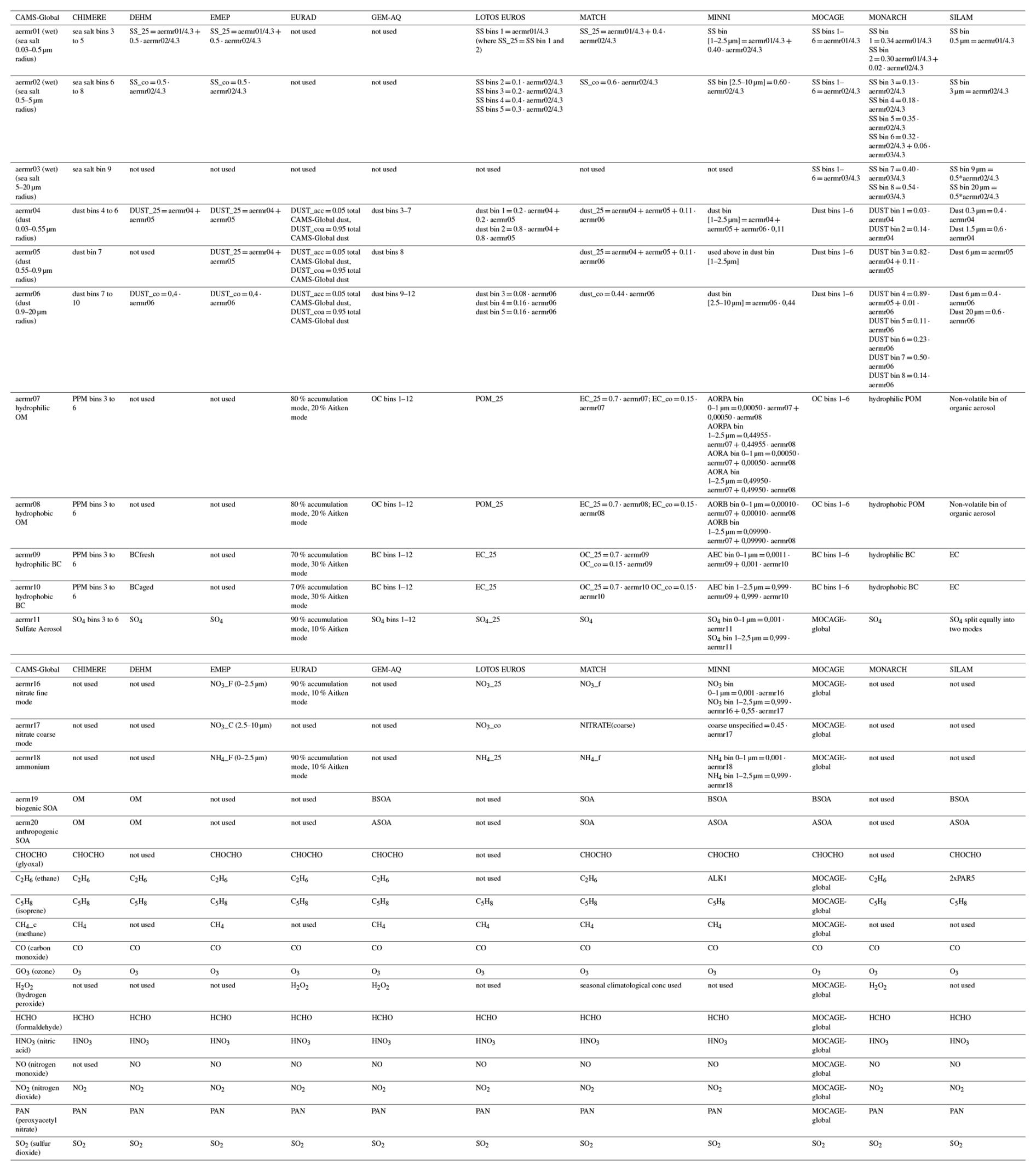
The list of species used as boundary conditions for the regional CAMS models is given in Table 2. Further details are available through the CAMS User Support website (https://confluence.ecmwf.int/display/CKB/CAMS%3A+Global+atmospheric+composition+forecast+data+documentation, last access: 8 September 2025) and Morcrette et al. (2009). All aerosol species are provided as dry PM, except for sea salt, whose mass and size and provided at a relative humidity of 80 %. The mass of the corresponding dry sea salt is $\mathrm{1}/\mathrm{4.3}$ smaller, and the radius is half of the sea salt at relative humidity of 80 %.

2.6 Surface emissions

2.6.1 Anthropogenic emissions

Using identical anthropogenic emissions in all the 11 individual models is essential for the consistency of the CAMS Regional products. The so-called TNO-MACC-III (Kuenen et al., 2014) emission inventory was used for several years in the past. Since June 2019, it has been replaced by the CAMS-REG emissions inventory, which is regularly updated (Kuenen et al., 2022). The CAMS-REG inventory is based on official national totals of air pollutant emissions reported in compliance with the European Directive on National Emission Reduction Commitments (2016/2284/EU, https://eur-lex.europa.eu/legal-content/EN/TXT/?uri=uriserv:OJ.L_.2016.344.01.0001.01.ENG&toc=OJ:L:2016:344:TOC, last access: 8 September 2025) and the Gothenburg Protocol of the LRTAP Convention. Additional processing is applied to ensure consistency in the dataset by making corrections and performing some gap filling where information is missing. A consistent spatial distribution for gridded emission datasets is applied at 0.05° × 0.1° resolution. Since June 2021, the CAMS Regional Production has used an improved version of the CAMS-REG inventory which substituted national estimates of wood burning emission in order to cope with a well-established inconsistency in the reporting of condensable emissions (Denier Van Der Gon et al., 2015).

The use of officially reported emissions induces a subsequent delay in the successive updates of the emission datasets. The emissions for year Y are reported in March Y+ 2. Then they undergo verification, gap filling and spatialisation before being considered for implementation in the CAMS Regional Production. The emissions being used for the day-to-day forecasts are thus generally based on national emissions reported about 3 years earlier. In order to cope with this limitation, the CAMS-REG emission inventory developed a methodology to extrapolate the officially reported emissions to the most recent historical year. The methodology basically consists in two steps. First, early available relevant activity data for different sectors are used to extrapolate the trend in the activity, which are used to adjust future emissions. Second, for the historical years for which emission data are available from CAMS-REG the trend in these is compared to the trend in the activities. If a significant trend is found (here defined as > 3 % per year), the trend in the implied emission factor is determined by taking the ratio of the trend in emissions and in activities, which is then projected into the future. The methodology has been validated for historical years and works well overall, but such a method also has limitations; for instance it is not possible to predict sudden events such as closure of power plants or industrial facilities or implementation of emission reduction techniques in large facilities. This way, the emission implemented in late 2024 in the Regional Production could be based on an estimate for the year 2023 (CAMS-REG v7.1).

The common requirement to use CAMS-REG emissions in all CTMs is strictly enforced for the forecast. For the analysis, in one of the models (Table 1) analysed concentrations are pulled away from the state that is physically related to the emissions and therefore will not be strictly relatable anymore to specified required emissions. But none of the models use inverse modelled emissions based on observation in the forecast.

Table 1 Overview of the main characteristics and configurations of the 11 chemistry-transport models as used in the CAMS Regional Production.

Only the spatialised annual fluxes of NO_x, SO_x, NMVOCs, NH₃, CO, PM₁₀, and PM_2.5 emissions are prescribed for all models. The subsequent disaggregation required in CTMs in terms of (i) hourly/daily/weekly/monthly profiles, (ii) vertical injection height, and (iii) mapping towards model chemical species is left open for individual modelling teams. Default information is nevertheless provided regarding the temporal disaggregation (Guevara et al., 2021) as well as the speciation of total VOC or total PM on individual VOC species or aerosol species, respectively. NMVOC emissions in CAMS-REG are provided with year-, sector-, and country-dependent speciation profiles to breakdown total NMVOCs to the 25 Global Emission InitiAtive (GEIA) species, originally defined under the REanalysis of the TROpospheric chemical composition (RETRO) project (Schultz et al., 2007). Each CAMS individual modelling team performs a remapping of the 25 GEIA NMVOC species to the species of their corresponding gas-phase chemical mechanism. Concerning PM, the default profiles provided in CAMS-REG allow splitting coarse and fine PM emissions to primary organic carbon, elemental carbon, sulfates, sodium, and others.

2.6.2 Biogenic, natural, and wildfire emissions

Biogenic emissions are left to the choice of individual operational models, most of which include their own online calculation of emissions from vegetation and other natural sources. They include soil emissions for (i) mineral dust resuspension, (ii) soil NO_x, or even (iii) sea salt within the European domain, but the agriculture-related NH₃ emissions are issued from the anthropogenic emission inventory.

The only coordination regarding ecosystem emissions concerns wildfires where all models are expected to use the Global Fire Assimilation System (GFAS) product (Kaiser et al., 2012) provided by CAMS. GFAS is based on fire radiative power retrievals from data of the Moderate Resolution Imaging Spectroradiometer (MODIS) instruments aboard the Terra and Aqua satellites. GFAS provides hourly emission data with a 8 h delay compared to real time. Each individual modelling team retrieves GFAS emission when initiating their forecast. As the individual forecasts are initiated between 12:00 D − 1 and 03:00 D + 0 depending on the regional systems, the only full day where GFAS wildfire emissions are available is D − 2, and some systems also include part of D − 1 emissions. Each system therefore reconstructs a 24 h cycle of emission based either on D − 2 only or also including part of D − 1 emissions. This cycle is used by all models for their analysis of D − 1. For the forecast, persistence of this daily cycle of emission is only maintained for D + 0 and D + 1 considering that the vast majority of wildfires in Europe are not persisting for longer time periods.

2.6.3 Pollen emission and dispersion

The following pollen species are included in the CAMS Regional Production: birch, grass, olive, ragweed, alder, and mugwort. Their implementation in the individual operational CAMS models differs in terms of advection and deposition strategies, but as for the anthropogenic air pollutants, the emission terms are coordinated following the original documentation of Sofiev et al. (2013) and subsequent updates for additional species. The pollen species differ in terms of their geographic distribution (source masks), total amount of available pollen grains, start and end date of the season (heat sum thresholds), and the shape of the season (source strength as function of time). The alder pollen emission model is similar to that of birch and olive, while the mugwort source is a variation of the grass source. However, mugwort is implemented as five different sub-species, each with its own spatially gridded start and end dates of the flowering season. Ragweed pollen follows the method described in Prank et al. (2013).

Once emitted, pollen species are advected in the model in the same way as other chemically inert species and are subject to gravitational settling and wet scavenging over time.

3 Individual model description

3.1 CHIMERE

3.1.1 Model overview

CHIMERE is a multi-scale CTM developed jointly by LMD, INERIS, and LISA (Menut et al., 2021). Its development was initiated in the early 2000s (Menut et al., 2000; Honoré et al., 2000), and it has since then pioneered operational national air quality forecasting in France (Rouïl et al., 2009). It is also extensively used for long-term simulations for emission control scenarios (Colette et al., 2013; Meleux et al., 2007; Colette et al., 2015). It runs over a range of spatial scale from the hemispheric to the urban scale, with resolutions from 100 to 1 km (Colette et al., 2014; Bessagnet et al., 2017). The exact model version used since June 2021 in the CAMS Regional Production is CHIMERE v2020r1.

3.1.2 Model geometry

For the CAMS Regional forecasts, CHIMERE uses a regular latitude–longitude grid with a 0.1° × 0.1° resolution, which covers 25° W to 45° E and 30 to 72° N and 9 vertical levels, extending from the surface up to 500 hPa, a lowermost layer about 20 m deep, and about seven layers below 2 km. No vertical downscaling is applied, and concentrations in the lowermost model layer are considered representative of the surface.

3.1.3 Forcing meteorology

The forcing meteorology is retrieved from the IFS model vertical layers covering the CHIMERE vertical extent on a 0.1° × 0.1° horizontal grid resolution with a temporal resolution of 3 h. The forecast released at 00:00 UTC of the previous days is used. The three-dimensional meteorological parameters included to force the CHIMERE forecast are horizontal wind components, temperature, specific humidity, orography, rainwater/snow mixing ratios, cloud liquid and ice water contents. The 2D variables included are surface temperature, surface pressure, large-scale and convective precipitations, boundary layer height, sensible and latent heat fluxes at surface, surface solar radiation downwards, and soil parameters (water and temperature) for four layers (0–7, 7–28, 28–100, 100–255 cm), sea ice cover, and snow depth.

3.1.4 Chemical initial and boundary conditions

Lateral and top boundary conditions are taken from chemical species available in CAMS-Global forecast model of the previous day at 3 h temporal resolution. The full list of species used from CAMS-Global is given in Table 2. The forecasts are initialised by the CHIMERE forecasts of the previous day.

3.1.5 Emissions

The common annual anthropogenic emissions CAMS-REG are implemented as explained in Sect. 2.5.1. Temporal disaggregation is based on TNO time profiles provided with CAMS-REG. Chemical disaggregation for VOCs is based on Passant (2002). PM components are speciated using the splits provided with the CAMS-REG database.

Biogenic VOC (BVOC) emissions are computed online with the MEGAN 2.10 algorithm (Guenther et al., 2012) implemented in CHIMERE and use high spatiotemporal data LAI (30 arcsec every 8 d) generated from MODIS (Yuan et al., 2011). Biogenic emission factors are estimated based on the 30 arcsec USGS (US Geophysical Survey) land-use database and the emission factors provided for each functional type by Guenther et al. (2012).

The hourly GFAS wildfire emission for D − 2 (i.e. the last full day available when launching the forecast system) are used for the analysis (D − 1) and the first 2 d of the forecast (D + 0 and D + 1). Fire emissions are set to zero for the remainder of the forecast horizon.

Dust production within the European domain is included. It is based on the dust production model optimised by Menut et al. (2005) using saltation (Marticorena and Bergametti, 1995) and cohesion kinetic energies scheme (Alfaro and Gomes, 2001).

3.1.6 Solver, advection, and mixing

The numerical time solver is based on a splitting operator which solves separately transport (including deposition and emissions), chemistry and aerosol formation.

Advection is based on the Piecewise Parabolic Method 3D order scheme (Colella and Woodward, 1984). Vertical turbulent mixing takes place only in the boundary layer. The formulation uses K-diffusion parameterisation (Troen and Mahrt, 1986), without counter-gradient term.

3.1.7 Deposition

Dry deposition of gaseous and particle species is parameterised as a downward flux out of the lowest model layer, where the deposition velocity is described through a resistance analogy (Wesely, 1989). Wet deposition of particles and gases is computed using a polydisperse distribution of rain droplets based on Willis and Tattelman (1989) and by computing the efficiency of the collision. Below-cloud scavenging of gases is assumed irreversible and is therefore only accounted for the most soluble compounds (HNO₃, H₂O₂, HCl, SO₂, and NH₃). In-cloud scavenging is accounted for all gases by computing the gaseous- and aqueous-phase partitioning based on Henry's law constants and the pH of the clouds. Scavenging by snow is also accounted for and is based on Chang (1984) for gases and on Wang et al. (2014) for particles.

3.1.8 Chemistry and aerosols

In order to optimise computing time, the reduced MELCHIOR2 mechanism with 44 species and about 120 reactions is derived from the full mechanism MELCHIOR (Derognat et al., 2003). The sectional aerosol module accounts for 7 species and 10 bins from 10 nm to 40 µm (primary particle material, nitrate, sulfate, ammonium, biogenic secondary organic aerosol SOA, anthropogenic SOA, and water). Photolytic rates are computed according to Mailler et al. (2016). The aerosol module is described in great detail in Couvidat et al. (2018) and accounts for condensation, nucleation, and condensation/evaporation. Aerosol thermodynamic equilibrium is achieved using the ISORROPIA model version 2.1. The secondary organic aerosol formation mechanism used in the operational forecasting version of CHIMERE is described in Bessagnet et al. (2008).

3.1.9 Assimilation system

The CHIMERE assimilation for operational purposes relies on a kriging-based approach to assimilate hourly concentration values for correcting the raw model results. For the analysis period, linear regression between a selected set of observations (excluding mountain and proximity sites) and the raw CHIMERE model is performed (in moving neighbourhood). The experimental variogram of the regression residuals is then computed, and a variogram model is fitted; the model adequacy is checked by cross-validation. Ultimately, observations are kriged with the CHIMERE model as external drift (in moving neighbourhood). This method is applied for O₃ and NO₂. For PM₁₀ and PM_2.5, an ordinary co-kriging of the observations (main variable) and CHIMERE (secondary variable) is applied to ensure consistency between both pollutants. Only in situ surface observations are used.

Further evolution of the CHIMERE assimilation system using an ensemble Kalman filter approach is under development, in particular to pave the way for assimilation of satellite data. It is has however not yet demonstrated that it provides a better skill score than the geostatistical method.

3.2 DEHM

3.2.1 Model overview

The Danish Eulerian Hemispheric Model (DEHM) is a 3-dimensional, offline, large-scale, Eulerian, atmospheric chemistry-transport model developed to study long-range transport of air pollution in the Northern Hemisphere. DEHM was originally developed in the early 1990s in order to study the atmospheric transport of sulfur dioxide and sulfate into the Arctic (Christensen, 1997; Heidam et al., 2004). The model has been modified, extended, and updated continuously since then and now includes a flexible setup with the possibility for nested domains with higher resolutions over targeted areas (Brandt et al., 2012; Geels et al., 2021). Apart from standard air pollution components and pollen, DEHM also includes mercury (Christensen et al., 2004), CO₂ (Lansø et al., 2019), and POPs (Hansen et al., 2008).

3.2.2 Model geometry

The horizontal domain is defined on a regular latitude–longitude grid of 0.1° resolution, with grid centre points covering longitudes 24.95° W to 44.95° E and latitudes 30.05 to 71.95° N. The vertical discretisation is defined on 29 terrain-following sigma levels up to about 100 hPa. The 12 lowest layers are within the lowest 1 km of the atmosphere, and the thickness of the lowest layer is about 20 m. The model includes an option for downscaling to the surface, but this is not applied in the operational setup.

3.2.3 Forcing meteorology

The forcing meteorology is retrieved from the IFS model vertical layers covering the DEHM vertical extent on a 0.2° × 0.2° horizontal grid resolution with a temporal resolution of 3 h. The forecast released at 12:00 UTC of the previous days is used. The meteorological parameters included to force the DEHM forecast are 3D fields of the horizontal wind components (U,V), temperature, specific humidity, cloud liquid water contents, cloud ice water contents, rain water contents, snow water contents, and fraction of cloud cover. The 2D fields are land–sea mask, surface pressure, geopotential height, skin temperature, U^*, large-scale and convective rain, snow depth, sensible heat flux, latent heat flux, net solar radiation, boundary layer height, 2 m temperature, 2 m dew point temperature, 10 m wind (U,V), albedo, sea ice area fraction, and surface roughness.

3.2.4 Chemical initial and boundary conditions

Lateral and top boundary conditions are taken from chemical species available in CAMS-Global forecast model of the previous day at 3 h temporal resolution. The full list of species used from CAMS-Global is given in Table 2. The DEHM forecasts are initialised by the DEHM forecasts of the previous day.

3.2.5 Emissions

The common annual anthropogenic emissions CAMS-REG are implemented as explained in Sect. 2.5.1. Originally the temporal disaggregation was based on the GENEMIS tables, using a GNFR-to-SNAP matrix. From 2021 the new CAMS-TEMPO (Guevara et al., 2021) profiles for annual, monthly, weekly, and daily distribution of emissions have been included in the operational version of DEHM. PM components are speciated using the splits provided with the CAMS-REG emissions. The speciation of VOCs from the emission input of total non-methane VOCs is based on the global speciated NMVOC emission database EDGAR 4.3.2 (Huang et al., 2017).

Natural emissions of the biogenic volatile organic compounds (BVOCs) isoprene and monoterpenes are estimated in DEHM based on the MEGAN model (Zare et al., 2012). The production of sea salt aerosols at the ocean surface is based on two parameterisation schemes describing the bubble-mediated sea spray production of smaller and larger aerosols. In each time step, the production is calculated for 10 size bins and thereafter summed up to give an aggregated production of fine (with dry diameters < 1.3 µm) and coarse (with dry diameters ranging 1.3–6 µm) aerosols (Soares et al., 2016). NO_x emissions from soil are based on data from the Global Emissions Inventory Activity (Yienger and Levy, 1995), and from lightning they are from Price et al. (1997).

The hourly GFAS wildfire emissions are retrieved as soon as they are available (i.e. with a 8 h delay from real time) in order to obtain a recent 24 h cycle spanning over D − 2 and D − 1. This cycle is used for the analysis (D − 1) and the first 2 d of the forecast (D + 0 and D + 1). Fire emissions are set to zero for the remainder of the forecast horizon. Hourly injection heights are calculated based on the hourly data of “mean altitude of maximum injection” and “altitude of plume top”.

3.2.6 Solver, advection, and mixing

The horizontal advection is solved numerically using the higher-order Accurate Space Derivatives scheme, documented to be very accurate (Dabdub and Seinfeld, 1994), especially when implemented in combination with a Forester filter (Forester, 1977). The vertical advection, as well as the dispersion sub-models, is solved using a finite-element scheme (Pepper et al., 1979) for the spatial discretisation. For the temporal integration of the dispersion, the Q method (Lambert, 1991) is applied, and the temporal integration of the 3-dimensional advection is carried out using a Taylor series expansion to third order. Time integration of the advection is controlled by the Courant–Friedrich–Lewy (CFL) stability criterion. A wind adjustment is included in order to ensure mass conservation.

The vertical diffusion is configured by K_z profiles (Hertel et al., 1995), based on Monin–Obukhov similarity theory for the surface layer. This K_z profile is extended to the whole boundary layer using a simple extrapolation, which ensures that K_z is decreasing in the upper part of the boundary layer. The planetary boundary layer (PBL) height is obtained directly from the IFS meteorology.

3.2.7 Deposition

Gaseous and aerosol dry deposition velocities are calculated based on the resistance method for 16 different land-use types and are configured similar to the EMEP model (Emberson et al., 2000b; Simpson et al., 2003), except for the dry deposition of species on water surfaces, where the deposition depends on the solubility of the chemical species and the wind speed (Hertel et al., 1995).

Wet deposition includes in-cloud and below-cloud scavenging and is calculated as the product of scavenging coefficients and the concentration of gases and particles in air (Simpson et al., 2003). The in-cloud scavenging coefficients are dependent on Henry's law constants and the rate at which precipitation is formed.

3.2.8 Chemistry and aerosols

The basic chemical scheme in DEHM now includes 74 different species and 158 reactions. It is based on the original scheme by Strand and Hov (1994). The original Strand and Hov scheme has been modified in order to improve the description of, amongst other things, the transformations of nitrogen containing compounds. The chemical scheme has been extended with a detailed description of the ammonia chemistry through the inclusion of ammonia (NH₃) and related species: ammonium-nitrate (NH₄NO₃), ammonium bisulfate (NH₄HSO₄), ammonium sulfate ((NH₄)₂SO₄) and particulate nitrate (NO₃) formed from nitric acid (HNO₃) using an aerosol equilibrium approach with reaction rates dependent on the equilibrium (Frohn, 2004). Furthermore, reactions concerning the wet-phase production of particulate sulfate have been included. The photolysis rates are calculated using a two-stream version of the Phodis model (Kylling et al., 1995). The original rates for inorganic and organic chemistry have been updated with rates from the chemical scheme applied in the EMEP model (Simpson et al., 2003). SOA formation is included via a volatility basis set (VBS)-based approach (Bergström et al., 2012; Zare et al., 2014). In total, DEHM includes nine classes of particulate matter (PM_2.5, PM₁₀, TSP, sea salt < 2.5 mm, sea salt > 2.5 mm, smoke from wood stoves, fresh black carbon, aged black carbon, and organic carbon).

3.2.9 Assimilation system

Since the system upgrade in November 2020, the assimilation in DEHM has been based on an updated version of the comprehensive 3D-Var data assimilation scheme previously described in Silver et al. (2016). The NMC method (Kahnert, 2008; Parrish and Derber, 1992) is used to estimate the background error covariance matrix. Two 1-year runs of DEHM using analysed and forecasted ECMWF weather data are performed, and their differences are used to estimate the background errors in spectral space for O₃, NO₂, SO₂, CO, PM_2.5, and PM₁₀. For the analysis and reanalysis runs, surface in situ observations of the six species are assimilated at an hourly basis in DEHM.

3.3 EMEP

3.3.1 Model overview

The EMEP MSC-W (European Monitoring and Evaluation Programme Meteorological Synthesizing Centre-West) model is a chemical transport model developed at the Norwegian Meteorological Institute under the EMEP programme of the United Nations Geneva Convention on Long-range Transboundary Air Pollution. The EMEP MSC-W model system allows several options with regard to the chemical schemes used and the possibility of including aerosol dynamics. Simpson et al. (2012) described an early version of the EMEP MSC-W model in detail, while updates to the model since 2012 have been documented and evaluated in the annual status reports of EMEP (see EMEP, 2023, and references therein). The forecast version of the EMEP MSC-W model (EMEP-CWF) has been in operation since June 2006. The scheduled model updates in CAMS ensure that the model version stays as close as possible to the official EMEP Open Source version (https://github.com/metno/emep-ctm, last access: 30 October 2024). Nevertheless, the EMEP-CWF results and performances in CAMS might differ from those presented in the annual EMEP Status Reports because of different input data (emissions and meteorological driver) and model configurations (Forecast in EMEP-CWF versus Hindcast in EMEP Status Reports).

3.3.2 Model geometry

The EMEP-CWF covers the European domain [30–76° N] × [30° W–45° E] on a geographic projection with a horizontal resolution of 0.1° × 0.1° (longitude–latitude). Vertically the model uses 20 levels defined as hybrid coordinates. The 10 lowest model levels are within the PBL, and the top of the model domain is at 100 hPa. The lowermost layer has a thickness of approximately 50 m. Vertical downscaling is used to derive surface concentrations at 3 m altitude, as described in Simpson et al. (2012).

3.3.3 Forcing meteorology

The forcing meteorology is retrieved from the IFS model vertical layers covering the EMEP vertical extent on a 0.1° × 0.1° horizontal grid resolution with a temporal resolution of 3 h. The forecast released at 12:00 UTC of the previous days is used. The meteorological parameters included to force the EMEP forecast are 3D fields of the horizontal wind components (U,V), potential temperature, specific humidity, and cloud fraction. The 2D fields are land–sea mask, surface pressure, friction velocity (u^*), large-scale and convective precipitation, soil water, snow depth, fraction of snow cover, fraction of ice cover, sensible heat flux, latent heat flux, sea surface temperature, 2 m temperature, and 2 m relative humidity. The IFS forecasts do not include 3D precipitation, which is needed by the EMEP-CWF model. Therefore, a 3D precipitation estimate is derived from large-scale precipitation and convective precipitation (surface variables).

3.3.4 Chemical initial and boundary conditions

Boundary conditions are taken from chemical species available in the CAMS-Global forecast model of the previous day at 3 h temporal resolution (Table 2). In cases where CAMS-Global chemical boundary conditions are not available, default boundary conditions are specified for O₃, CO, NO, NO₂, CH₄, HNO₃, PAN, SO₂, isoprene, C₂H₆, some VOCs, sea salt, Saharan dust, and SO₄, as annual mean concentrations along with a set of parameters for each species describing seasonal, latitudinal, and vertical distributions. It should be noted however that unavailability of CAMS-Global is very exceptional (less than once a year) and in general due to data transfer issues. The EMEP forecasts are initialised by the EMEP 3D VAR analysis of the previous day.

3.3.5 Emissions

The common annual anthropogenic emissions CAMS-REG are implemented as explained in Sect. 2.5.1. Temporal disaggregation is based on CAMS-REG-TEMPO v4.1. Chemical disaggregation for PM species follows the tables that come with CAMS-REG, while VOC emissions are speciated for each source sector based on a lumped-species approach as described in Simpson et al. (2012) and Bergström et al. (2022).

The hourly GFAS wildfire emissions for D − 2 (i.e. the last full day available when launching the forecast system) are used for the analysis (D − 1) and the first 2 d of the forecast (D + 0 and D + 1). Fire emissions are set to zero for the remainder of the forecast horizon.

The mineral dust source in the EMEP model is based on Alfaro and Gomes (2001), Fécan et al. (1999), Gomes et al. (2003), Marticorena and Bergametti (1995), and Marticorena et al. (1997).

Natural emissions of biogenic volatile organic compounds (BVOCs) are based on Table 3 of Simpson et al. (2012).

3.3.6 Solver, advection, and mixing

The numerical solution of the advection terms of the continuity equation is based on the scheme of Bott (1989). The fourth-order scheme is utilised in the horizontal directions. In the vertical direction, a second-order version applicable to variable grid distances is employed.

The turbulent diffusion coefficients (K_z) are first calculated for the whole 3D model domain on the basis of local Richardson numbers. The planetary boundary layer (PBL) height is then calculated using methods described in Simpson et al. (2012). For stable conditions, K_z values are retained. For unstable situations, new K_z values are calculated for layers below the mixing height using the O'Brien interpolation.

3.3.7 Deposition

Parameterisation of dry deposition is based on a resistance formulation. The deposition module makes use of a stomatal conductance algorithm, which was originally developed for ozone fluxes but which is now applied to all gaseous pollutants when stomatal control is important (Emberson et al., 2000a; Simpson et al., 2003; Tuovinen et al., 2004). Non-stomatal deposition for NH₃ is parameterised as a function of temperature, humidity, and the molar ratio SO${}_{\mathrm{2}}/{\mathrm{NH}}_{\mathrm{3}}$.

Both gaseous and particulate nitrogen species are scavenged in the EMEP model according to their wet scavenging ratios and collection efficiencies listed in Table S20 of Simpson et al. (2012). In-cloud and sub-cloud scavenging ratios are considered for gases and in-cloud scavenging ratios and sub-cloud scavenging efficiencies for particles.

3.3.8 Chemistry and aerosols

The EmChem19 chemical scheme couples the sulfur and nitrogen chemistry to the photochemistry and organic aerosol formation using about 200 reactions between ca. 130 species (Bergström et al., 2022; Simpson et al., 2020b; Andersson-Sköld and Simpson, 1999). The standard model version distinguishes two size fractions for aerosols, fine aerosol (PM_2.5) and coarse aerosol (PM_2.5–10). The aerosol components presently accounted for are SO₄, NO₃, NH₄, anthropogenic primary PM, organic aerosols, and sea salt. Also, aerosol water is calculated. Dry deposition parameterisation for aerosols follows standard resistance formulations, accounting for diffusion, impaction, interception, and sedimentation. Wet scavenging is treated with simple scavenging ratios, taking into account in-cloud and sub-cloud processes. For secondary organic aerosol (SOA) a volatility-basis set approach (Simpson et al., 2012) is used, which is a somewhat simplified version of the mechanisms discussed in detail by Bergström et al. (2012). The EmChem19a scheme also has explicit toluene and benzene with different SOA yields to the o-xylene surrogate that was used previously.

3.3.9 Assimilation system

The EMEP data assimilation system (EMEP-DAS) is based on the 3D-Var implementation for the MATCH model (Kahnert, 2008). The background error covariance matrix is estimated following the NMC method (Parrish and Derber, 1992). Recent changes involved increased computational efficiency, tuning of model and observation representation uncertainties, and improved impact of the assimilation in the vertical.

The EMEP-DAS delivers analyses of D − 1 (driven by the operational IFS forecast of 00:00 UTC of yesterday) assimilating O₃, NO₂, CO, PM_2.5, and PM₁₀ surface observations.

3.4 EURAD-IM

3.4.1 Model overview

The EURAD-IM (European Air pollution Dispersion – Inverse Model) system consists of five major parts: the meteorological driver WRF (Weather Research and Forecasting (https://www.mmm.ucar.edu/models/wrf, last access: 30 October 2024), the pre-processors EEP and PREP for preparation of anthropogenic emission data and observations, the EURAD-IM Emission Model (EEM), and the chemistry-transport model EURAD (Hass et al., 1995; Memmesheimer et al., 2004). EURAD-IM is a Eulerian mesoscale chemistry-transport model involving advection, diffusion, chemical transformation, wet and dry deposition and sedimentation of tropospheric trace gases and aerosols. It includes 3D-Var and 4D-Var chemical data assimilation (Elbern et al., 2007) and is able to run in nesting mode.

3.4.2 Model geometry

To cover the CAMS domain from 25° E to 45° W and 30 to 72° N, two Lambert conformal projections subdomains with respectively 45 km (199 × 166 grid boxes) and 9 km horizontal resolution (581 × 481 grid boxes) are used. The model domain with the finer resolution covering the entire European part of the CAMS domain is nested within the halo domain with the coarser resolution.

Variables are horizontally staggered using an Arakawa C-grid. Vertically, the atmosphere is divided by 23 terrain-following sigma coordinate layers between the surface and the 100 hPa pressure level. About 15 layers are within the first 2 km of the atmosphere The thickness of the lowest layer is about 35 m. No vertical downscaling is used to derive surface concentrations from the first model level.

3.4.3 Forcing meteorology

The meteorological forcing is obtained from 3-hourly IFS forecasts, but unlike the other models, the Weather Research and Forecast (WRF) model is used to compute meteorological fields on the grid needed to drive the EURAD-IM CTM. This intermediate processing is essentially for historical reasons as in the past the IFS temporal and spatial resolution required interpolation for use in the CTM. A direct use of the IFS data to dynamically drive EURAD-IM has been developed and is currently in testing to enter operational production in the near future.

3.4.4 Chemical initial and boundary conditions

The CAMS-Global 00:00 UTC forecast for the previous day is extracted from the MARS archive at ECMWF using 36 model levels with a temporal resolution of 3 h. The full list of species used from the CAMS-Global model is given in Table 2. Sea salt concentrations from CAMS-Global are divided by the constant 4.3 for the conversion from wet to dry mass.

3.4.5 Emissions

The common annual anthropogenic emissions CAMS-REG are implemented as explained in Sect. 2.5.1. The VOC and PM split, the vertical distribution of area sources, and the emission strength per hour are calculated within the EURAD-IM CTM with the distribution profiles provided with the CAMS-REG-AP_v6.1/2019 inventory (Kuenen et al., 2022). The VOC and PM split depends on source category and country; the vertical distribution only depends on the source category. The CAMS-TEMPO v4.1 (Guevara et al., 2021) profiles are used for the annual, monthly, weekly, and daily distribution of emissions.

Biogenic emissions and NO_x emissions from soil are calculated within the EURAD-IM CTM with MEGAN (Guenther et al., 2012). Fire emissions are taken into account using hourly data from the GFASv1.2 product (Kaiser et al., 2012). Zero fire emissions are assumed for D + 2 and D + 3 forecasts.

Table 2 Overview of the matching between chemical species used as boundary conditions from the CAMS-Global model and the 11 regional models of the CAMS Regional Production.

3.4.6 Solver, advection, and mixing

The positive definite advection scheme of Bott (1989), implemented in a one-dimensional realisation, is used to solve the advective transport. An operator splitting technique is employed (McRae et al., 1982) to handle the varying numerical specificities of processes to be solved.

An eddy diffusion approach is used to parameterise the vertical sub-grid-scale turbulent transport. The calculation of vertical eddy diffusion coefficients is based on the specific turbulent structure in the individual regimes of the planetary boundary layer (PBL) according to the PBL height and the Monin–Obukhov length (Holtslag and Nieuwstadt, 1986). A semi-implicit (Crank–Nicolson) scheme is used to solve the diffusion equation.

The sub-grid cloud scheme in EURAD-IM was derived from the cloud model in the EPA Models-3 Community Multiscale Air Quality (CMAQ) modelling system (Roselle and Binkowski, 1999). Convective cloud effects on both gas-phase species and aerosols are considered.

3.4.7 Deposition

The gas-phase dry deposition modelling follows the method proposed by Zhang et al. (2003). Dry deposition of aerosol species is treated depending on size, using the resistance model of Petroff and Zhang (2010) with consideration of the canopy. Dry deposition is applied as lower boundary condition of the diffusion equation.

Wet deposition of gases and aerosols is derived from the cloud model in the CMAQ modelling system (Roselle and Binkowski, 1999). The wet deposition of pollen is treated according to Baklanov and Sørensen (2001).

Size-dependent sedimentation velocities are calculated for aerosol and pollen species. The sedimentation process is parameterised with the vertical advective transport equation and solved using the fourth-order positive definite advection scheme of Bott (1989).

3.4.8 Chemistry and aerosols

In the EURAD-IM CTM, the gas-phase chemistry is represented by an extension of the Regional Atmospheric Chemistry Mechanism (RACM) (Stockwell et al., 1997) based on the Mainz Isoprene Mechanism (MIM) (Geiger et al., 2003). A two-step Rosenbrock method is used to solve the set of stiff ordinary differentials equations (Sandu and Sander, 2006). Photolysis frequencies are derived using the FTUV model (fast TUV) according to Tie et al. (2003). The radiative transfer model therein is based on the Tropospheric Ultraviolet-Visible Model (TUV) developed by Madronich and Weller (1990).

The modal aerosol dynamics model MADE (Ackermann et al., 1998) is used to provide information on the aerosol size distribution and chemical composition. To solve for the concentrations of the secondary inorganic aerosol components, a FEOM (fully equivalent operational model) version, using the HDMR (high-dimensional model representation) technique (Nieradzik, 2005; Rabitz and Aliş, 1999), of an accurate mole-fraction-based thermodynamic model (Friese and Ebel, 2010) is used. The updated SORGAM module (Li et al., 2013) simulates secondary organic aerosol formation.

3.4.9 Assimilation system

The EURAD-IM assimilation system (Elbern et al., 2007) includes (i) the EURAD-IM CTM and its adjoint, (ii) the formulation of both background error covariance matrices for the initial states and the emission and their treatment to precondition the minimisation problem, (iii) the observational basis and its related error covariance matrix, and (iv) the minimisation including the transformation for preconditioning. The quasi-Newton limited-memory L-BFGS algorithm described in Liu and Nocedal (1989) and Nocedal (1980) is applied for the minimisation.

Currently assimilated in the EURAD-IM analysis and interim reanalysis are surface in situ observations of O₃, NO₂, SO₂, CO, PM_2.5, and PM₁₀.

3.5 GEM-AQ

3.5.1 Model overview

GEM-AQ is a numerical weather prediction model where air quality processes (gas phase and aerosols) are implemented online in the host meteorological model, the Global Environmental Multiscale (GEM) model, developed at Environment and Climate Change Canada (Côté et al., 1998a). The model is used for operational air quality forecasting in Poland. Also, it is used in a research project to investigate air quality in different environmental conditions (Struzewska and Kaminski, 2008, 2012; Struzewska et al., 2015, 2016).

3.5.2 Model geometry

The GEM-AQ model can be configured to simulate atmospheric processes over a broad range of scales, from the global scale down to the meso-gamma scale. An arbitrarily rotated latitude–longitude mesh focuses resolution on any part of the globe. In the CAMS Regional Production, the model is run in the limited-area mode with a resolution of 0.1° × 0.1° on a spherical coordinate system. The coordinates are the following: lower-left (17.4° N/22.1° W), upper-right (58.6° N/86.6° E). In the vertical, GEM-AQ uses the generalised sigma vertical coordinate system. It has terrain-following sigma surfaces near the ground that transform to pressure surfaces higher in the atmosphere. The model top is set at 10 hPa.

3.5.3 Forcing meteorology

The operational IFS model provides meteorological fields for the initial and boundary conditions used by the meteorological part of the GEM-AQ model. The GEM-AQ model is started using the 12 h forecast (valid at 00:00 UT of the following day) as the initial conditions. The IFS data are used as boundary conditions with a nesting interval of 3 h. The IFS meteorological fields are computed from spectral coefficients for the target GEM-AQ grid. Meteorological fields, in the GEM-AQ model domain, are constrained within the nesting zone (absorber), which is defined over 10 grid points on each lateral boundary of the limited area domain.

3.5.4 Chemical initial and boundary conditions

Chemical species of the CAMS-Global forecast for the previous day are used with a temporal resolution of 3 h (Table 2). For dust aerosols, the three available size bins from the CAMS-Global model are distributed uniformly over the 10 corresponding bins in GEM-AQ. For organic matter aerosol, black carbon, and sulfates, the same log-normal-based profile was applied. For organic aerosol and black carbon, hydrophobic and hydrophilic components were summed as “total organic aerosol” and “total black carbon aerosol” before applying size-bin distribution profiles.

3.5.5 Emissions

The common annual anthropogenic emissions CAMS-REG are implemented as explained in Sect. 2.5.1. Based on this information, emission fluxes for 15 gaseous species (9 hydrocarbons and 6 inorganics) and 4 aerosol components (primary organic aerosol, black carbon, sulfates, nitrates) are derived using factors provided by TNO. Total emission fluxes for each aerosol component are distributed into 12 bins in the GEM-AQ aerosol module.

Anthropogenic emissions are distributed within the seven lowest model layers (up to 1350 m) with injection height profiles for each of the GNFR sectors re-mapped for the GEM-AQ levels (Bieser et al., 2011). Temporal profiles modulating annual and diurnal variation of emission fluxes for each GNFR are used.

For biogenic emissions, a temperature-dependent, monthly averaged MEGAN-MACC (Sindelarova et al., 2014) dataset for the year 2010 was used specifically to avoid the short-term variability of reactive biogenic VOCs that would otherwise be generated in an online approach. In contrast to the online method, this approach provides an anticipated variability range, particularly by reducing the influence of online factors such as meteorological errors and extreme values.

3.5.6 Solver, advection, and mixing

The set of non-hydrostatic Eulerian equations (with a switch to revert to the hydrostatic primitive equations) maintains the model's dynamical validity right down to the meso-gamma scales. The time discretisation of the model dynamics is a fully implicit, two-time-level scheme (Côté et al., 1998b, a). The spatial discretisation for the adjustment step employs a staggered Arakawa C-grid that is spatially offset by half a mesh length in the meridional direction. It is of second-order accuracy, whereas the interpolations for the semi-Lagrangian advection are of fourth-order accuracy.

Deep convective processes are handled by Kain–Fritsch convection parameterisation (Kain and Fritsch, 1990). The vertical diffusion of momentum, heat, and tracers is a fully implicit scheme based on turbulent kinetic energy (TKE) theory.

3.5.7 Deposition

The effects of dry deposition are included as a flux boundary condition in the vertical diffusion equation. Dry deposition velocities are calculated from a “big leaf” multiple resistance model (Wesely, 1989; Aamaas et al., 2013) with an aerodynamic, quasi-laminar layer and surface resistances acting in series. The process assumes 15 land-use types and takes snow cover into account. Wet deposition takes into account cloud scavenging for soluble gas species and aerosols.

3.5.8 Chemistry and aerosols

The gas-phase chemistry mechanism currently used in the GEM-AQ model is based on a modification of version 2 of the Acid Deposition and Oxidants Model (ADOM) (Venkatram et al., 1988), derived from the condensed mechanism of Lurmann et al. (1986). The ADOM-II mechanism comprises 47 species, 98 chemical reactions, and 16 photolysis reactions. In order to account for background tropospheric chemistry, 4 species (CH₃OOH, CH₃OH, CH₃O₂, and CH₃CO₃H) and 22 reactions were added. All species are solved using a mass-conserving implicit time stepping discretisation, with the solution obtained using Newton's method. Heterogeneous hydrolysis of N₂O₅ is calculated using the online distribution of aerosol. Although the model meteorology is calculated up to 10 hPa, the focus of the chemistry is in the troposphere where all species are transported throughout the domain. To avoid the overhead of stratospheric chemistry, the ozone and NO_y fields are replaced above 100 hPa with those from the CAMS-Global model. Additionally, stratospheric columns for absorbing species used in photolysis calculations (cf., ozone) are taken from the CAMS-Global model. Photolysis rates (J values) are calculated online every chemical time step using the method described in Landgraf and Crutzen (1998). In this method, radiative transfer calculations are done using a two-stream approximation for eight spectral intervals in the UV and visible applying pre-calculated effective absorption cross sections. This method also allows for scattering by cloud droplets and for clouds to be presented over a fraction of a grid cell. The host meteorological model provides both cloud cover and water content. The J value package used was developed for MESSy (Jöckel et al., 2006) and is implemented in GEM-AQ.

The current version of GEM-AQ has five size-resolved aerosol types, viz. sea salt, sulfate, black carbon, organic carbon, and dust as well as nitrates. The microphysical processes that describe the formation and transformation of aerosols are calculated by a sectional aerosol module (Gong et al., 2003). The particle mass is distributed into 12 logarithmically spaced bins from 0.005 to 10.24 µm radius. This size distribution leads to an additional 60 advected tracers. The following aerosol processes are accounted for in the aerosol module: nucleation, condensation, coagulation, sedimentation and dry deposition, in-cloud oxidation of SO₂, in-cloud scavenging, and below-cloud scavenging by rain and snow.

3.5.9 Assimilation system

Data assimilation in the GEM-AQ modelling system is done with the optimal interpolation method (Robichaud and Ménard, 2014) and is applied to the forecast. Error statistics are computed with the Hollingsworth–Lönnberg (HL) method (Hollingsworth and Lönnberg, 1986). It estimates the correlation length and the ratio of observation to model error variances by a least-squares fit of a correlation model against the sample of the spatial autocorrelation of observation-minus-model residuals.

Currently, data assimilation is done at each forecast hour for O₃, NO₂, SO₂, CO, PM₁₀, and PM_2.5, using surface observations.

3.6 LOTOS-EUROS

3.6.1 Model overview

The LOTOS-EUROS model is a 3D chemistry-transport model aimed to simulate air pollution in the lower troposphere. The model has been used in a large number of studies for the assessment of particulate air pollution and trace gases (e.g. O₃, NO₂) (Hendriks et al., 2016; Schaap et al., 2013; Thürkow et al., 2021; Timmermans et al., 2022). A detailed description of the model is given in Manders et al. (2017). At present the version used in the production is v2.2.009.

3.6.2 Model geometry

The domain of LOTOS-EUROS is the CAMS Regional domain from 25° W to 45° E and 30 to 72° N. The projection is regular longitude–latitude, at 0.1° × 0.1° grid spacing. In the vertical and for the forecasts there are currently 12 model layers and two more reservoir layers at the top, defined by coarsening in a mass conservative way the first 77 model levels of the IFS. For output purposes, the concentrations at measuring height (usually 2.5 m) are diagnosed by assuming that the flux is constant with height and equal to the deposition velocity times the concentration at height z (taken as average over the grid cell). This applies for several of the gaseous species, namely O₃, NO, NO₂, HNO₃, N₂O₅, H₂O₂, CO, SO₂, and NH₃. For aerosols, the same approach is utilised, except sedimentation velocity is used instead of deposition velocity.

3.6.3 Forcing meteorology

The forcing meteorology is retrieved from the 00:00 and 12:00 UTC runs of the IFS model at hourly (surface fields) or 3-hourly temporal resolution (model layer fields). The meteorological data are retrieved on a regular horizontal resolution of about 9 km and for all layers covered by the model's vertical extent. The meteorological variables included are 3-hourly 3D fields for wind direction, wind speed, temperature, humidity, and density, augmented by hourly 2D gridded fields of mixing layer height, surface wind and temperature, precipitation rates, heat fluxes, cloud cover and surface variables' snow depth, sea ice cover, and volumetric soil water.

3.6.4 Chemical initial and boundary conditions

The lateral and top boundary conditions for trace gases and aerosols are obtained from the CAMS-Global daily forecasts (see Table 2). LOTOS-EUROS uses a bulk approach for the aerosol size distribution differentiating between a fine and a coarse fraction, but for dust and sea salt there are five distinct size classes: ff: 0.1–1 µm, f: 1–2.5 µm, ccc: 2.5–4 µm, cc: 4–7 µm, c: 7–10 µm. When the chemical boundary conditions from CAMS-Global are missing (which is very rare, typically less than once a year, and can, for example, be due to delays in the file transfer or other serious technical issues at ECMWF), the model uses climatological boundary concentrations derived from CAMS-Global data. The forecasts are initialised with the LOTOS-EUROS forecast of the previous day.

3.6.5 Emissions

The common annual anthropogenic emissions CAMS-REG are implemented as explained in Sect. 2.5.1. Injection height distribution from the EuroDelta study is implemented, which is per SNAP (or more recently, GNFR) category. Time profiles used are defined per country and GNFR emission category type.

Biogenic NMVOC emissions are calculated online using actual meteorological data and a detailed land-use and tree species database including emission factors from Köble and Seufert (2001). The isoprene emissions follow the mathematical description of the temperature and light dependence of the isoprene emissions, proposed by Guenther et al. (1993). Sea salt emissions are parameterised following Martensson et al. (2003) and Monahan (1986) from the wind speed at 10 m height.

The fire emissions are taken from the near-real-time GFAS fire emissions database. For the forecast, we assume persistence, so the latest downloaded emission for the specific hour is used. When the hourly emission is more than 3 d old, it is set to zero.

Mineral dust emissions within the modelling domain are calculated online based on the sand blasting approach by Marticorena and Bergametti (1995), with soil moisture inhibition as described by Fécan et al. (1999). Finally, a parameterisation using land cover and temperature is used for handling soil NO_x emissions, based on Yienger and Levy (1995).

3.6.6 Solver, advection, and mixing

The transport consists of advection in three dimensions, horizontal and vertical diffusion, and entrainment/detrainment. The advection is driven by meteorological fields (u,v), which are input every 3 h. The vertical wind speed w is calculated by the model as a result of the divergence of the horizontal wind fields. A linear advection scheme is used to ensure tracer mass conservation, which also allows more efficient parallelisation and reduced model complexity. This scheme uses piece-wise linear functions to define sub-grid concentrations, which is sometimes referred to as MUSCL (“Monotonic Upwind-centred Scheme for Conservation Laws”) following van Leer (1984).

Vertical diffusion is described using the standard K_z theory. Vertical exchange is calculated employing the new integral scheme by Yamartino et al. (2007). For the forecasting set-up with 12 layers, atmospheric stability values and functions, including K_z values, are derived based on the surface heat fluxes from ECMWF meteorology and similarity profiles following the IFS approach (ECMWF, 2021) to adapt for land-use-specific conditions. For the 5-layer version in the assimilation, a correction is made for the vertical diffusion to correct for the height difference between the surface and mixing layer.

3.6.7 Deposition

The dry deposition in LOTOS-EUROS is parameterised following the resistance approach. The laminar layer resistance and the surface resistances for acidifying components are described following the EDACS system (Van Zanten et al., 2010), and the deposition velocities for particles are based on Zhang et al. (2001). Wet deposition is divided between in-cloud and below-cloud scavenging. The in-cloud scavenging module is based on the approach described in Seinfeld and Pandis (1998) and Banzhaf et al. (2012).

3.6.8 Chemistry and aerosols

LOTOS-EUROS uses the TNO CBM-IV scheme, which is a modified version of the original CBM-IV (Gery et al., 1989). N₂O₅ hydrolysis is described explicitly based on the available (wet) aerosol surface area (using γ= 0.05) (Schaap et al., 2004). Aqueous-phase and heterogeneous formation of sulfate is described by a simple first-order reaction constant (Barbu et al., 2009; Schaap et al., 2004). Inorganic aerosol chemistry is represented using ISORROPIA II (Fountoukis and Nenes, 2007), and secondary organic aerosol formation based on a VBS scheme (Bergström et al., 2012; Zare et al., 2014) will be included in the operational forecast version in the future.

3.6.9 Assimilation system

The LOTOS-EUROS model is equipped with a data assimilation package with the ensemble Kalman filter technique (Curier et al., 2012). The ensemble is created by specification of uncertainties for emissions (NO_x, VOC, NH₃, and aerosol), ozone deposition velocity, and ozone top boundary conditions. Currently, data assimilation is performed for O₃, NO₂, PM₁₀, and PM_2.5 surface observations, and OMI NO₂ is also assimilated.

3.7 MATCH

3.7.1 Model overview

The Multi-scale Atmospheric Transport and Chemistry model (MATCH) (Robertson et al., 1999) is an offline chemical transport model (CTM) with a flexible design, accommodating different weather data forcing on different resolutions and projections and a range of alternative schemes for deposition and chemistry.

3.7.2 Model geometry

The model's geometry is taken from the input weather data. To reduce computational costs, the vertical resolution is reduced compared to the ECMWF operational model by merging pairs of IFS vertical layers, while retaining the use of hybrid vertical coordinates. The horizontal resolution in the MATCH simulation matches that of the meteorological forcing, which is currently provided on a 0.1° latitude–longitude grid. The lowest 78 layers of the ECMWF model are lumped in 39 levels, which then are used for the air quality simulations. The model top is at about 8000 m height. The model domain covers the area between 28.8° W to 45.8° E and 29.2 to 72.0° N. The grid is an Arakawa C-grid with staggered wind components.

3.7.3 Forcing meteorology

The forcing meteorology for MATCH forecasts is retrieved from the 12:00 UTC run of the IFS modelling system on a 0.1° × 0.1° spatial grid and with a temporal resolution of 3 h. For the analyses, the 00:00 UTC analysis of the IFS is used at 0.2° × 0.2° resolution. The reason for applying a coarser resolution in the analysis is twofold: (1) the delivery time is rather short from when the in situ observations are available, and (2) the analysis increments are on a larger scale. The meteorological variables included are 3D fields of the horizontal wind components (U,V), temperature, specific humidity, cloud cover, cloud water content, cloud ice water content, and surface fields of surface pressure, logarithm of surface pressure, surface temperature, sea surface temperature, snow depth, albedo, roughness height, total cloud cover, precipitation, and volumetric soil water at the surface.

3.7.4 Chemical initial and boundary conditions

The lateral boundary conditions for trace gases and aerosols are obtained from the CAMS-Global forecasts at 3-hourly resolution for the following species: O₃, CO, HCHO, NO, NO₂, SO₂, HNO₃, PAN, CH₄, C₅H₈, o-xylene, sulfate, and C₂H₆ (see Table 2). In the event that the chemical boundary conditions from CAMS-Global would be missing (which has never happened in practice but could in theory happen due to due to corruption or other technical issues), the model uses seasonal climatological boundary concentrations instead.

3.7.5 Emissions

The common annual anthropogenic emissions CAMS-REG are implemented as explained in Sect. 2.5.1. Temporal disaggregation is based on the GENEMIS tables (Ebel et al., 1997), using a GNFR-to-SNAP matrix. The vertical distribution of the emissions depends on the sector. Near-surface emission sources (SNAP 2, 6, 7, 8, 10) are distributed in the lowest 90 m; for other sectors the emissions are allocated over varying model levels up to a maximum of about 1100 m height. According to the sector, the anthropogenic VOC emissions are split into the MATCH chemical mechanism surrogate species: C₂H₆, NC₄H₁₀, C₂H₄, C₃H₆, o-xylene, benzene, toluene, CH₃OH, C₂H₅OH, HCHO, CH₃CHO, and CH₃COC₂H₅; the particulate matter components elemental carbon, organic matter, and anthropogenic dust (other than soil and road dust) are allocated to two bins (PM_2.5 and PM coarse); the road dust estimated according to Manders et al. (2009) and Omstedt et al. (2005); and the telluric dust calculated according to Zender et al. (2003).

Biogenic emissions of isoprene, monoterpenes, and sesquiterpenes are calculated following Simpson et al. (2012, 1995) and Bergström et al. (2012), taking into account temperature at 2 m, radiation fluxes, and the vegetation cover.

The dimethyl sulfide – DMS – emissions from the ocean and Baltic Sea are also considered, whereas the particulate matter from sea salt is calculated according to the parameterisation proposed by Sofiev et al. (2011).

The GFAS biomass burning emissions are taken into the model mapping the following species into the MATCH chemical mechanism: NO_x, SO₂, CO, CH₄, C₂H₄, C₂H₆, C₃H₆, C₄H₁₀, C₈H₁₀, benzene, toluene, CH₃OH, C₂H₅OH, formaldehyde, acetaldehyde, OC, BC, PM_2.5, and PM₁₀. The vertical injection is made by a parabolic curve, with central height taken from the GFAS INJH parameter. In case the injection height is missing for a GFAS emission cell, this is assigned from some neighbour height present. The diurnal emission profile is based on the D − 1 GFAS hourly data filled up with GFAS data for D − 2 for the not-yet-available hours in D − 1. This diurnal hourly profile is repeated throughout the forecast.

3.7.6 Solver, advection, and mixing

Mass conservative transport schemes are used for advection and turbulent transport. The advection is formulated as a Bott-like scheme (Robertson et al., 1999). A second-order transport scheme is used in the horizontal as well as the vertical. The vertical diffusion is described by an implicit mass conservative first-order scheme, where the exchange coefficients for neutral and stable conditions are parameterised following Holtslag and Nieuwstadt (1986). In the convective case, the turbulent Courant number is directly determined from the turnover time in the boundary layer.

Part of the dynamical core is the initialisation and adjustment of the horizontal wind components. This is a very important step to ensure mass conservative transport. The initialisation is based on a procedure proposed by Heimann and Keeling (1989), where the horizontal winds are adjusted by means of the difference between the input surface pressure tendency, and the calculated pressure tendency is assumed to be an error in the divergent part of the wind field.

Boundary layer parameterisation is based on surface heat and water vapour fluxes as described by Van Ulden and Holtslag (1985) for land surfaces and Burridge (1977) for sea surfaces. The boundary layer height is calculated from formulations proposed by Zilitinkevich and Mironov (1996) for the neutral and stable case and from Holtslag et al. (1995) for the convective case. These parameterisations drive the formulations for dry deposition and vertical diffusion.

3.7.7 Deposition

Dry deposition of gases and aerosols is modelled using a resistance approach (based on the scheme in Simpson et al., 2012), which includes stomatal and non-stomatal pathways for vegetated surfaces. In the current operational system, the model applies this scheme across various physiographic tiles derived from the CLC/SEI inventory (https://www.sei.org/projects/sei-european-land-cover-map, last access: 30 October 2024, Simpson et al., 2012). MATCH uses 3D precipitation (estimated in the model, based on the surface precipitation and 3D cloud water information from the IFS forecast) and separates wet scavenging into in-cloud and sub-cloud scavenging. For most gaseous components the scavenging is assumed to be proportional to the precipitation intensity (with higher scavenging ratios in-cloud than sub-cloud). For the particulate components in-cloud scavenging is also treated using simple scavenging ratios, while the sub-cloud scavenging is treated using a scheme based on Berge (1993) with size-dependent collection efficiencies (as in Simpson et al., 2012).

3.7.8 Chemistry and aerosols

The photochemistry scheme is based on the EMEP MSC-W chemistry scheme (Simpson et al., 2012), with a modified scheme for isoprene, based on the so-called Carter-1 mechanism (Carter, 1996; Langner et al., 1998). The standard MATCH setup used in CAMS treats particles as bulk aerosol in two size classes, fine (PM_2.5) and coarse (PM_2.5–10) particles. Particle formation from gases includes secondary inorganic aerosol (ammonium sulfate and nitrate) and secondary organic aerosol. Ammonium nitrate equilibrium is calculated according to Mozurkewich (1993). Coarse nitrate formation from gas-phase HNO₃ is also included (Strand and Hov, 1994). Secondary organic aerosol formation from oxidation of volatile organic compounds is treated using a volatility basis set scheme based on Hodzic et al. (2016). Exception is made for the isoprene oxidation for which the chain of reactions is following the Carter-1 chemical mechanism, which has proven to give comparable results with fewer reactions (Carter, 1996; Langner et al., 1998).

3.7.9 Assimilation system

The model for data assimilation is an integrated part of the MATCH modelling system. The data assimilation scheme as such is a variational spectral scheme (Kahnert, 2008), implying that the background covariance matrices are modelled in spectral space. The limitation is that covariance structures are described as isotropic and homogeneous. The advantage is that the background error matrix becomes block diagonal, and there are no scale separations as the covariance between spectral components is explicitly handled. The block diagonal elements are the covariance between wave components at model layers and chemical compounds.

Modelling the background error covariance matrices is the central part in data assimilation. This is conducted by means of the so-called NMC approach (Parrish and Derber, 1992). The CTM (MATCH) is run for a 3-month period for photochemistry and aerosols with analysed and forecasted ECMWF weather data. The differences are assumed to mimic the background errors, and the statistics in spectral space are generated for different combinations of the model compounds: O₃, NO₂, NO, SO₂, CO, PM_2.5, and PM₁₀.

The scheme is fully intermittent in hour-by-hour steps and the above-listed components are assimilated from in situ measurements. The analysed components are propagated by chemistry and transport into unobserved components as NMVOCs, PAN, and NH₃.

3.8 MINNI

3.8.1 Model overview

MINNI (Italian Integrated Assessment Modelling System for supporting the International Negotiation Process on Air Pollution and assessing Air Quality Policies at national/local level; D'Elia et al., 2021; Mircea et al., 2014) has been developed to support the Italian Ministry for Environment and Territory and Sea. The core of the modelling system is the 3-dimensional offline Eulerian CTM FARM (Flexible Air quality Regional Model (Silibello et al., 2008), which accounts for the transport, chemistry, and removal of atmospheric pollutants.

3.8.2 Model geometry

For the CAMS Regional forecast, the model is configured with a regular latitude–longitude grid of 0.15° × 0.10° resolution. The domain spans −25 to 45.05° E and 30 to 72° N. The model uses z-level terrain-following mesh with the first central grid point at 20 m a.g.l. (above ground level) and the last one at 6290 m a.g.l. No vertical downscaling is applied to extrapolate concentrations from 20 m above the ground to the surface.

3.8.3 Forcing meteorology

The forcing meteorology is retrieved from the 12:00 UTC run of the IFS modelling system on a 0.1° × 0.1° spatial grid and with a temporal resolution of 1 h. The meteorological variables included are 3D fields such as temperature, relative humidity, pressure, and wind velocity and 2D fields such as boundary layer height, roughness length, albedo, sea surface temperature, total cloud cover, and precipitation.

3.8.4 Chemical initial and boundary conditions

The lateral and top boundary conditions for trace gases and aerosols are obtained from the CAMS-Global daily forecasts with a 3 h temporal resolution (see Table 2). The initial condition is taken from the previous forecast of the MINNI model.

3.8.5 Emissions

The common annual anthropogenic emissions CAMS-REG are implemented as explained in Sect. 2.5.1. Point emissions are summed up to gridded emissions for each GNFR sector, since no information was available about the characterisation of the point sources in terms of injection height. Conservative mass horizontal interpolation has been applied to map the emissions on the actual model domain. Vertical splitting has been applied for each GNFR sector, adapting the vertical injection profiles provided by TNO to the actual model levels. Temporal emission profiles for each GNFR sector, as they were provided by TNO, have been applied considering local time (i.e. the time zone shift has been taken into account).

PM_2.5 has been speciated following the TNO table as a function of country and sector and AERO3 (Binkowski and Shankar, 1995; Binkowski, 1999) species size fractions below 2.5 µm. The coarse component (PM₁₀–PM_2.5) was associated with the non-speciated coarse mode since MINNI dispersion model considers all the secondary aerosol fraction to be PM_2.5. This method leaves the detailed chemical speciation out but ensures mass conservation.

The NMVOC speciation originated from the TNO table as a function of country and sector obtaining the v01–v25 species. The mapping among the v01–v25 species to SAPRC99 species has been done in agreement with the choices made and tested in the frame of EURODELTA III intercomparison exercise (Colette et al., 2017).

Biogenic emissions are computed with the MEGAN model v.2.04 (Guenther et al., 2006) and NO_x emissions from soil following Williams et al. (1992) approach.

Erosion and resuspension of the dust are calculated by means of method proposed by Vautard et al. (2005). Road dust emissions are parameterised following Zender et al. (2003).

Fire emissions are taken into account using hourly data from the GFAS database considering emissions from D − 1 for AN (D − 1) and FC (D + 0 and D + 1, zero for the remaining days).

3.8.6 Solver, advection, and mixing

FARM is a 3-dimensional Eulerian model with first-order turbulence closure. Physical and chemical processes influencing the concentration fields within the modelling domain are described by a system of partial differential equations (PDEs). The numerical integration of the above system of PDEs is performed by a method that splits the multi-dimensional problem into time-dependent one-dimensional problems, which are then solved sequentially over the time step.

Partial differential equations involved in horizontal and vertical advection–diffusion operators are solved in FARM using the schemes employed in CALGRID model (Yamartino et al., 1992). In particular, horizontal advection–diffusion operators are solved using a finite-element method based on Blackman cubic polynomials. The coefficients of a cell-centred cubic polynomial are constrained to maintain high-accuracy and low-diffusion characteristics and to avoid undesirable negative concentrations. In addition, a filter is used for filling undesired short wavelength minima. The numerical integration of the vertical diffusion equation is performed in a hybrid way employing a hybrid semi-implicit Crank–Nicolson/fully implicit scheme (Yamartino et al., 1992).

The calculation of horizontal diffusion coefficients is based on stress tensor formulation of Smagorinsky (1963) also including a dependence on the local stability class and wind speed. For the calculation of vertical diffusion coefficients, the Lange (1989) approach to boundary layer scaling regimes is used. Mixing due to deep convection is not explicitly taken into account.

Two different schemes to compute the PBL scaling parameters are used. In the daytime, the Maul et al. (1980) version of Carson (1973) encroachment method is used. During nighttime, the minimum value between Nieuwstadt (1981) and Venkatram (1980) is used.

3.8.7 Deposition

The dry deposition velocities are modelled following a resistance analogy approach, as an inverse sum of a series of three resistances: the aerodynamic resistance, the quasi-laminar layer resistance, and the surface resistance. Aerodynamic resistance is dependent on surface characteristics and atmospheric stability conditions (described through friction velocity and Monin–Obukhov length). Quasi-laminar layer resistance is parameterised using Hicks et al. (1987). Surface resistance is approximated as a set of parallel resistance associated with leaf stomata, leaf cuticles, lower canopy and surface soil, litter, and water (Wesely, 1989). Deposition to water surfaces is based on Slinn et al. (1978).

The deposition velocity of particulate species also depends on particle size distribution and density because of gravitational settling. Sedimentation velocity acts in parallel to the other resistances. Hygroscopic growth is considered over water for particles less than 2 µm. For particles ranging from 0.1 to 1 µm, deposition velocity is computed as the inverse of the resistance computed from canopy height, friction velocity, and Monin–Obukhov length.

The parameterisation of wet deposition follows the Simpson et al. (2012) approach, including in-cloud and below-cloud scavenging of gas and particles.

3.8.8 Chemistry and aerosols

The gas-phase chemical mechanism used for CAMS forecast is SAPRC-99, with the inclusion of polycyclic aromatic hydrocarbons (PAHs) and mercury chemistry; moreover, a simplified aqueous-phase mechanism is included for SO₂ oxidation and chemical processes involving mercury in both gas and aqueous phases.

A simple approach is used to estimate photolysis rates based on look-up tables to calculate the rate constants for photolysis reactions (Nenes et al., 1998). Photolysis rates are computed and adjusted according to local solar zenith angle using an empirical formula based on Peterson (1976) data.

The aerosol module is AERO3 (Binkowski and Shankar, 1995; Binkowski, 1999). In AERO3 the representation of the particle size is three-modal (Aitken, accumulation, and coarse), following lognormal distributions. The aerosol species included are sulfate, nitrate, ammonium, anthropogenic primary and secondary organic aerosol, biogenic secondary organic aerosol, elemental carbon, sea salt, and dust. The aerosol dynamics takes into account nucleation, condensation, and coagulation processes. The gas–particle mass transfer is implemented by means of ISORROPIA v1.7 (Nenes et al., 1998) and SORGAM (Schell et al., 2001a) for secondary inorganic and organic aerosol, respectively.

3.8.9 Assimilation system

The assimilation scheme used is optimal interpolation: the correlation function is factorised in vertical and horizontal components. The horizontal component has pollutant-dependent fixed correlation length with a terrain-following exponential decay. The vertical component is modelled with a Cressman function dependent on the boundary layer height. The system assimilates NO₂, O₃, SO₂, CO, PM₁₀, and PM_2.5. In the case of aerosol components, the correction applied to each of them is proportional to their content in PM. At present, only data from surface stations are assimilated. More details are available in Adani and Uboldi (2023).

3.9 MOCAGE

3.9.1 Model overview

The MOCAGE 3D multi-scale chemistry and transport model has been designed for both research and operational applications in the field of environmental modelling. Since 2000, MOCAGE has been allowed to cover a wide range of topical issues, ranging from chemical weather forecasting, tracking and backtracking of accidental point source releases, trans-boundary pollution assessment, and assimilation of remote sensing measurements of atmospheric composition to studies of the impact of anthropogenic emissions of pollutants on climate change (Guth et al., 2018; Cussac et al., 2020).

3.9.2 Model geometry

For the CAMS Regional Service, MOCAGE operates on a regular latitude–longitude grid at 0.1 resolution covering the 28 to 72° N and 26° W to 46° E domain, for both forecast and assimilation. The products delivered for the CAMS service are issued from the regional domain only. In the vertical, 47 hybrid levels go from the surface up to 5 hPa, with approximately 8 levels in the planetary boundary layer (i.e. below 2 km), 16 in the free troposphere, and 24 in the stratosphere. The thickness of the lowest layer is about 40 m. There is no downscaling applied to surface concentration.

3.9.3 Forcing meteorology

The forcing meteorology is retrieved from the IFS model vertical layers covering the MOCAGE vertical extent on a 0.1° × 0.1° horizontal grid resolution with a temporal resolution of 1 h for the first 3 forecast days and 3 h for the last forecast day. The forecast released at 12:00 UTC of the previous days is used. The meteorological parameters used for the dynamics calculation in MOCAGE are horizontal and vertical winds, temperature, humidity, cloud fraction, surface pressure, albedo, precipitation, and incoming radiative flux. The variables relevant for the deposition module are soil humidity and temperature, wind speed and direction, specific humidity, pressure at ground level, and sensible heat flux.

3.9.4 Chemical initial and boundary conditions

Chemical initial values in the regional domain are provided by the MOCAGE 24 h forecast from the day before. The boundary conditions are taken from global CAMS operational suite for the species (chemical and aerosols) that are distributed (see Table 2). For aerosols, the 2 or 3 bins from CAMS-Global are summed to get total concentration and then distributed onto the 6 MOCAGE bins considering Mean CAMS-Global bin size as emission modes. A factor of 4.3 is applied to convert sea salt from wet to dry fractions. Aerm03 (of diameter larger than 10 µm) is only marginally distributed within MOCAGE PM₁₀ sea salt because of the matching between bins and log-normal modes. For the species not included in Table 2, the concentrations from the MOCAGE global domain are used, which helps to introduce these chemical boundary conditions smoothly into the CAMS Regional domain, on the horizontal as well as on the vertical.

3.9.5 Emissions

The common annual anthropogenic emissions CAMS-REG are implemented as explained in Sect. 3.2. Temporal disaggregation is based on the GENEMIS tables (Ebel et al., 1997), using a GNFR to SNAP matrix. Chemical disaggregation for PM species and VOCs is based on sector- and country-dependent split factors proposed by TNO.

Isoprene biogenic emissions are computed online using the MEGAN model (Guenther et al., 2012), while other biogenic emissions are computed from the CAMS global biogenic emission inventory (version 3.1). NO_x soil emissions are taken from the CAMS-GLOB-SOILv2.2 emission inventory.

Concerning biomass burning sources, GFAS emissions are emitted according to an “umbrella” profile, with a maximum injecting height climatologically determined. GFAS “near-real-time” observation-based fire emissions are made available with a 8 h delay. Therefore, when the forecast system is initiated, most GFAS emission cover D −2 of the forecast to be produced. As a consequence, the 2 d persistence is interpreted in a way that fire emissions are only applied for D + 0.

3.9.6 Solver, advection, and mixing

The chemical solver used is a semi-implicit solver as presented in Cariolle and Teyssèdre (2007).

Concerning physical and chemical parameterisations, an operator splitting approach is used. Parameterisations are called alternatively in forward and reverse order, with the objective to reduce systematic errors.

Meteorological forcings are read every 3 h from IFS input data and are linearly interpolated to yield hourly values, which is the time step for advection; smaller time steps are used for physical processes and chemistry, but the meteorological variables are kept constant over each hour. MOCAGE is based upon a semi-Lagrangian advection scheme (Williamson and Rasch, 1989), using a cubic polynomial interpolation in all three directions.

For sub-grid-scale transport processes, vertical diffusion is treated following Louis (1979), and transport by convection is from Bechtold et al. (2001). Scavenging within convective clouds is following Mari et al. (2000), allowing wet removal processes to be computed directly within the convective transport parameterisation.

3.9.7 Deposition

Wet deposition in stratiform clouds and below clouds follows Giorgi and Chameides (1986). A description of MOCAGE surface exchanges module is presented in Michou et al. (2005). The dry deposition parameterisation relies on a fairly classical surface resistance approach (Wesely, 1989) but with a refined treatment of the stomatal resistance, similar to the one used in Meteo-France numerical weather prediction models (Noilhan and Planton, 1989). Sedimentation of aerosol follows Nho-Kim et al. (2004).

3.9.8 Chemistry and aerosols

The MOCAGE configuration for CAMS comprises 118 species and over 300 reactions and photolysis. It is a merge of reactions of the RACM scheme (Stockwell et al., 1997), with the reactions relevant to the stratospheric chemistry of REPROBUS (Lefevre et al., 1994). Aqueous chemistry for the formation of sulfate is represented, following Ménégoz et al. (2009). Detailed heterogeneous chemistry on polar stratospheric clouds (types I, II) is accounted for, as described in Lefevre et al. (1994). Other heterogeneous chemistry processes are currently not included.

Photolysis is taken into account using a multi-entry lookup table computed offline with the TUV software version 4.6 (Madronich, 1987). Photolysis depends on month (including monthly aerosol climatologies), solar zenith angle, ozone column above each cell (as the model extends to the mid-stratosphere, it is actually the ozone profile computed by MOCAGE which is used at every time step), altitude, and surface albedo in the UV. They are computed for clear-sky conditions, and the impact of cloudiness on photolysis rates is applied afterwards.

The aerosol module of MOCAGE includes the primary species dusts, black carbon, sea salt, and organic carbon and the secondary inorganic species sulfate, nitrate, and ammonium. The formation and the multi-phasic equilibrium of inorganic secondary aerosols are modelled by the ISORROPIA-II module. Details on MOCAGE aerosol simulation evaluation can be found in Martet et al. (2009) for dusts, in Nho-Kim et al. (2005) for black carbon, and in Siè et al. (2015) for the latest version of MOCAGE primary aerosol module. The implementation and the evaluation of secondary inorganic aerosols in MOCAGE are described by Guth et al. (2016). Further improvements of the representation of aerosols in MOCAGE are expected in the future with ongoing work regarding organic secondary aerosols.

3.9.9 Assimilation system

MOCAGE operations for CAMS use the assimilation system based upon MOCAGE and PALM (Lahoz et al., 2007). As a first approximation, background error standard deviations are prescribed as proportional to background amounts. In order to spread assimilation increments spatially, background error correlations are modelled using a generalised diffusion operator (Weaver and Courtier, 2001). Several assimilation strategies are available in PALM, but for CAMS MOCAGE uses a 3D-VAR technique, with an assimilation window that is 1 h every hour.

For surface analyses (NRT, IRA, and VRA), MOCAGE assimilates O₃, NO_2, CO, PM₁₀, and PM_2.5 in situ surface observations. The species are assimilated independently every hour without any cross-species covariances, and then the increments per species are added to the analysis that serves at initial condition for computing the background of the next hour of the assimilation process, in this reanalysis mode.

An hourly assimilation cycle is also used to update the atmospheric state of aerosols, with the assimilation of French lidars (mini-MPL) and some ceilometers from the European network E-profile in the regional domain of MOCAGE. The quantity modified during the assimilation process is the 3D field of total mass of all aerosol types and all sizes all together. The split per aerosol type and particle size is not modified during the assimilation. This hourly assimilation cycle is the backbone, and every day at 00:00  UTC, the +96 h forecast is initialised from this assimilation cycle.

3.10 MONARCH

3.10.1 Model overview

The MONARCH model is a fully online multiscale chemical weather prediction system for regional and global-scale applications (Badia and Jorba, 2015; Badia et al., 2017; Jorba et al., 2012; Klose et al., 2021a; Pérez et al., 2011). The system is based on the meteorological Nonhydrostatic Multiscale Model on the B-grid (NMMB; Janjic and Gall, 2012), developed and widely verified at the National Center for Environmental Prediction (NCEP). The model couples the NMMB online with the gas-phase and aerosol continuity equations to solve the atmospheric chemistry processes in detail. The model is designed to account for the feedbacks among gases, aerosol particles and meteorology. Currently, it can consider the direct radiative effect of aerosols while ignoring cloud–aerosol interactions.

3.10.2 Model geometry

The hybrid pressure–sigma coordinate is used in the vertical direction, and the Arakawa B-grid is applied in the horizontal direction. The regional model is formulated on a rotated longitude–latitude grid, with the Equator of the rotated system running through the middle of the integration domain, resulting in more uniform grid distances. In the operational regional CAMS forecasts, the model is configured for a regional domain covering Europe and part of northern Africa with a regular horizontal grid spacing on the rotated projection of 0.15° (lower-left corner at 16.37° N 22.14° W, upper-right corner at 58.56° N 88.18° E), and the top of the domain is set at 50 hPa using 24 vertical layers. Surface concentrations of gases and aerosols are derived directly from the first model level; no particular vertical downscaling is implemented. The depth of the first vertical layer of the model is around 45 m, and about seven layers are set below 2 km.

3.10.3 Forcing meteorology

The forcing meteorology is retrieved from the IFS model on a 0.125° × 0.125° horizontal grid resolution (the native resolution is remapped as close as possible to the MONARCH grid to optimise transfer time), with a temporal resolution of 6 h and dynamically interpolated to the final chemistry grid and time steps using the meteorological component of MONARCH. The IFS forecast released at 12:00 UTC of the previous days is used. The meteorological variables obtained from IFS are skin temperature, soil temperature, soil moisture, snow depth, sea ice mask, sea-level pressure, U component of the wind, V component of the wind, temperature, geopotential height, relative humidity or specific humidity, and cloud water content.

3.10.4 Chemical initial and boundary conditions

The variables used from chemical species available in the CAMS-Global forecast model are detailed in Table 2. Note that CH₄ is not used from CAMS-Global because the MONARCH chemical mechanism considers a constant CH₄ concentration of 1.85 ppmv. A remapping has been applied to couple the modal distribution of the CAMS-Global aerosols with the aerosol distribution of the MONARCH model (see Table 2). The forecasts are initialised by the model results of the previous day.

3.10.5 Emissions

The common annual anthropogenic emissions CAMS-REG are implemented as explained in Sect. 2.5.1. The High-Elective Resolution Modelling Emission System version 3 (HERMESv3; Guevara et al., 2019) is used to pre-process the anthropogenic, ocean, and biomass burning emissions for the MONARCH model. HERMESv3 is an open-source, parallel and stand-alone multiscale atmospheric emission modelling framework that processes gaseous and aerosol emissions for use in atmospheric chemistry models.

CAMS_REG-AP NMVOC and PM_2.5 emissions are speciated using the sector- and country-dependent split factors proposed by TNO. In terms of NO_x, a fraction of 90 % NO and 10 % NO₂ is considered for all sectors except for road transport, in which the following fractions are applied: (i) 95 % NO, 4.2 % NO₂, and 0.8 HONO for petrol road transport and (ii) 70 % NO, 28.3 % NO₂, and 1.7 % HONO for diesel road transport (Rappenglück et al., 2013). The vertical distribution of anthropogenic emissions is performed following the sector-dependent profiles proposed by TNO. The temporal distribution follows the gridded CAMS-REG-TEMPO v4.1 profiles (Guevara et al., 2021).

The biogenic emissions for NMVOCs and NO are computed online within the MONARCH model using the Model of Emissions of Gases and Aerosols from Nature version 2.04 (MEGANv2.04; Guenther et al., 2006), while monthly oceanic emissions of DMS are obtained from the CAMS-GLOB-OCEA v3.1 dataset (Granier et al., 2019; Lana et al., 2011).

Mineral dust emissions can be calculated online using one of the schemes described in Klose et al. (2021a). For sea salt aerosol emissions, multiple source functions are available (Spada et al., 2013).

Finally, biomass burning emissions (forest, grassland and agricultural waste fires) of organic carbon, black carbon, SO₂, and DMS are taken from the GFASv1.4 dataset. This product reports hourly emissions at a horizontal gridded resolution of 0.1° × 0.1°. The vertical allocation of GFAS emissions is done using the maximum fire plume injection height and distributing all the emissions uniformly across the layers below this height. The persistence of the fires in forecast mode is set to 2 d; afterwards biomass burning emissions are set to zero.

3.10.6 Solver, advection, and mixing

Different chemical processes were implemented following a modular operator splitting approach to solve the advection, diffusion, emission, dry and wet deposition, and chemistry processes. In order to maintain consistency with the meteorological solver, the chemical species are advected and mixed at the corresponding time step of the meteorological tracers following the principles described in Janjic and Gall (2012) and references therein. The advection scheme is Eulerian, positive definite and monotone, maintaining a consistent mass conservation of the chemical species within the domain of study. Lateral diffusion is formulated following the Smagorinsky non-linear approach, while vertical diffusion is based on the Mellor–Yamada–Janjic level 2.5 turbulence closure scheme.

The convective mixing, however, is treated differently for aerosols and gases. The scheme implemented for aerosols is described in detail in Pérez et al. (2011) and follows a relaxation approach similar to the Betts–Miller–Janjic convective parameterisation of the NMMB. On the other hand, the convective mixing of gases is solved following the sub-grid cloud scheme of Foley et al. (2010) as described in Badia et al. (2017).

3.10.7 Deposition

The deposition processes implemented in the MONARCH model are dry deposition, in-cloud grid-scale, and in-cloud subgrid-scale scavenging for gases and aerosols and below-cloud scavenging for aerosols only.

For gases, the dry deposition scheme follows the classical deposition velocity analogy, enabling the calculation of deposition fluxes from airborne concentrations. The canopy resistance is simulated following Wesely (1989). The cloud-chemistry processes are included in the system considering both the sub-grid and grid-scale scheme described in Foley et al. (2010). The processes included are the scavenging, vertical mixing, and wet deposition. Only in-cloud scavenging is considered in the current implementation (Badia et al., 2017).

Regarding aerosols, the parameterisation of the aerosol dry deposition is based on Zhang et al. (2001), which includes simplified empirical parameterisations for the deposition processes of Brownian diffusion, impaction, interception, and gravitational settling. Wet scavenging of aerosols by precipitation is computed separately for convective and grid-scale (stratiform) precipitation. The model includes parameterisations for in-cloud scavenging and for below-cloud scavenging. A detailed description of the schemes can be found in Pérez et al. (2011).

3.10.8 Chemistry and aerosols

A gas-phase module combined with a hybrid sectional-bulk mass-based aerosol module is implemented in the MONARCH model. The gas-phase chemical mechanism used is the Carbon Bond 2005 chemical mechanism (CB05; Yarwood et al., 2005) extended with chlorine chemistry (Sarwar et al., 2012). The rate constants were updated based on evaluations from Atkinson et al. (2004) and Sander et al. (2006). The photolysis scheme used is the Fast-J scheme (Wild et al., 2000). It is coupled with physics of each model layer (e.g. aerosols, clouds, absorbers as ozone), and it considers grid-scale clouds from the atmospheric driver.

The aerosol module in the MONARCH model solves the life cycle of sea salt, dust, organic matter (both primary and secondary), black carbon, sulfate, and nitrate aerosols. While a sectional approach is used for dust and sea salt, a bulk description of the other aerosol species is adopted. A simplified gas–aqueous–aerosol mechanism accounts for sulfur chemistry (Spada, 2015). The production of secondary nitrate–ammonium aerosol is solved using the thermodynamic equilibrium model EQSAM (Metzger et al., 2002). The coarse nitrate production is computed with an uptake reaction of HNO₃ on dust and sea salt coarse particles. The formation of SOA is considered using a simple non-volatile scheme accounting for the contribution of anthropogenic, biomass burning, and biogenic formation (Pai et al., 2020). Hygroscopic growth is considered for all aerosol components except mineral dust.

3.10.9 Assimilation system

The MONARCH assimilation system (MONARCH-DA) is based on a local ensemble transform Kalman filter (LETKF) scheme (Di Tomaso et al., 2022; Di Tomaso et al., 2017; Escribano et al., 2022; Hunt et al., 2007; Miyoshi and Yamane, 2007; Schutgens et al., 2010) coupled to the model through I/O routines. The MONARCH ensemble is created by perturbing anthropogenic, biomass burning, soil, and ocean emissions that are pre-processed by HERMESv3 or that are modelled by MONARCH via a physically based scheme for dust aerosol. For analysis production in CAMS, the MONARCH ensemble is run at a horizontal resolution of 0.2° latitude × 0.2° longitude in a rotated grid and initialised by the ensemble forecast of the previous day.

Hourly surface observations from in situ measurements are currently assimilated operationally for O₃, NO₂, SO₂, CO, PM₁₀, and PM_2.5. For near-real-time operational analysis production, previous-day observations are combined with a MONARCH 24 h ensemble forecast initialised at 12:00 UTC of the previous day.

3.11 SILAM

3.11.1 Model overview

The System for Integrated modeLling of Atmospheric coMposition SILAM (https://silam.fmi.fi, last access: 8 September 2025) is a global-to-sub-kilometre chemistry-transport model developed for a wide range of atmospheric composition and air quality assessment tasks (Sofiev et al., 2015b), emergency decision support applications (Sofiev et al., 2008), and data assimilation and source inversion problems (Vira and Sofiev, 2015; Sofiev et al., 2013). The model incorporates Eulerian and Lagrangian dispersion frameworks (the Eulerian transport routine is used for CAMS) and a set of chemical and physical transformation modules for the troposphere and the stratosphere (Carslaw et al., 1995; Damski et al., 2007; Yarwood. G. et al., 2005; Sofiev, 2000; Sofiev et al., 2010). Apart from the transport and physico-chemical cores described below, SILAM includes a set of supplementary tools including a meteorological pre-processor, input-output converters, reprojection, and interpolation routines. In the operational forecasts, these enabled direct forcing of the model by the ECMWF IFS meteorological fields.

SILAM has been extensively evaluated in a variety of regional and global air quality projects (Brasseur et al., 2019; Huijnen et al., 2010; Kouznetsov et al., 2020; Petersen et al., 2019; Sofiev et al., 2015b; Xian et al., 2019) and health impact assessment studies (Korhonen et al., 2008; Kukkonen et al., 2020; Lehtomäki et al., 2018).

3.11.2 Model geometry

The centre points of the model grid cover 25.05° W to 44.95° E and 30.05 to 71.95° N on a regular latitude–longitude grid of 0.1° resolution. Following Sofiev (2002), SILAM uses a multi-vertical approach with the meteorology-resolving grid corresponding to the tropospheric part of the IFS vertical: hybrid levels from 69 to 137. The chemical transformations and vertical fluxes are computed based on 10 thick staggered layers, with the thickness increasing from 25 m for the lowest layer to 1000–2000 m in the free troposphere. The layer tops are located at 25, 75, 175, 375, 775, 1500, 2700, 4700, 6700, and 8700 m above the surface. Within the thick layers, the sub-grid information is used to evaluate the weighted averages of the high-resolution meteorological parameters and effective diffusion coefficients after Sofiev (2002).

3.11.3 Forcing meteorology

Meteorological forcing is the ECMWF IFS operational forecasts taken from the 12:00 UTC forecast of the previous day extracted at a resolution of 0.1° and temporal frequency of 1 h for the first 72 h and 3 h for the last day of the forecast. The list of meteorological parameters extracted is U and V components of 10 m wind [m s⁻¹], 2m temperature [K], dew point temperature 2 m [K] accumulated large-scale rain [kg m⁻²], accumulated convective rain [kg m⁻²], surface roughness [m], total cloud cover [fract], convective available potential energy [J kg⁻¹], U and V wind components at model levels [m s⁻¹], temperature at model levels [K], cloud water at model levels [kg kg⁻¹], cloud ice at model levels [kg kg⁻¹], specific humidity at model levels [kg kg⁻¹], cloud cover at model levels [fract], and logarithm of surface pressure.

3.11.4 Chemical initial and boundary conditions

Boundary conditions are taken from the CAMS-Global (see Table 2). The full fields are imported every 3 h; in between, the linear interpolation is applied. The forecasts are initialised with the SILAM forecast of the previous day.

3.11.5 Emissions

The common annual anthropogenic emissions CAMS-REG are implemented as explained in Sect. 3.2. The PM_2.5 emissions are split into EC, OC, and mineral components, and OC is mapped to the volatility bins according to Shrivastava et al. (2008). Emissions of biogenic VOCs, wind-blown dust, and sea salt are computed online in dedicated SILAM modules (Poupkou et al., 2010; Sofiev et al., 2011; Soares et al., 2016; Sofieva et al., 2022). GFAS hourly emissions from wild-land fires are replicated from D − 2 to D + 1 for forecast and shut down after; in the analysis mode it is used as is.

Emissions of six pollen species are computed online following the heat-sum approach for trees (Sofiev et al., 2015b), climatological season for grasses and mugwort species, and multi-criteria hybrid model for ragweed (Prank et al., 2013).

3.11.6 Solver, advection, and mixing

The SILAM Eulerian transport core (Sofiev et al., 2015a) is based on the coupled developments: refined advection scheme of Galperin and Sofiev (Sofiev, 2000) and vertical diffusion and dry deposition algorithm of Sofiev (2002) and Kouznetsov and Sofiev (2012). The methods are compatible, in a sense that both use the same set of variables to determine the sub-grid distribution of tracer mass. The approach, in particular, allows correct vertical exchange to be computed using high-resolution input data but low-resolution chemistry and diffusion grids. The latter feature is used in the vertical setup with thick layers.

Diffusion is parameterised following the first-order K-theory-based closure. Horizontal diffusion is embedded into the advection routine, which itself has zero numerical viscosity, thus allowing full control over the diffusion fluxes. The vertical diffusivity parameterisation follows the approach suggested by Groisman and Genikhovich (1997) and Sofiev et al. (2010). The procedure diagnoses all the similarity theory parameters using the profiles of the basic meteorological quantities: wind, temperature, and humidity. Output includes the value of eddy diffusivity for scalars at some reference height (taken to be 1 m).

The model uses process-wise splitting and 1D advection implementation, flipping the order of processes every other time step.

3.11.7 Deposition

Dry deposition parameterisation for gases generally follows the resistive analogy of Wesely (1989). Deposition velocities for aerosols are evaluated using the original Kouznetsov and Sofiev (2012) algorithm. Wet deposition parameterisation is based on the scavenging coefficient after Sofiev (2000) for gas species and follows the generalised formulations of Kouznetsov and Sofiev (2012) for aerosols.

3.11.8 Chemistry and aerosols

The main gas-phase chemical mechanism is CB05 with additions for SO_x from Sofiev (2000) and organics from a VBS approach (Shrivastava et al., 2008). The heterogeneous scheme is an updated version of the DMAT model scheme (Sofiev, 2000). The formation pathways of secondary inorganic aerosols follow the VBS approach extended with the feedback to the main gas-phase chemical module. The aerosol size distribution is represented via a sectional approach, with species-specific bin selections. Each bin is characterised with its lower and upper borders, as well as the mass-mean diameter, which is precomputed/predefined for each bin and species from its size spectrum. Primary anthropogenic aerosols are emitted into bins with mass-mean diameter of 0.5 µm (fine aerosol, dry size) and 6 µm (coarse aerosols, dry size). Secondary inorganic aerosols were put into 0.2 and 0.7 µm bins and a separate 3 µm bin for coarse nitrates formed on the sea salt surface. The dust size spectrum is described with 4 bins from 0.3 up to 20 µm. Finally, the sea salt spectrum is represented with 5 bins, from 0.05 up to 20 µm of mass-mean nominal diameter. Throughout computations, the particles are transported in accordance with their mass-mean diameter corrected with regard to actual humidity and the particle solubility. External mixing is assumed.

3.11.9 Assimilation system

The embedded data assimilation is based on the 3D- and 4D-dimensional variational approach, as well as the EnKF (Vira and Sofiev, 2012, 2015). Tangent-linear (if needed) and adjoint formulations exist for the transport module, the transformation schemes, and the deposition modules. The assimilation procedure has been tested for both initialising the concentration fields and for refining the emission (Sofiev, 2019). The observation operators exist for in situ observations and for the vertically integrated columns observed by the nadir-looking satellites. For the near-real-time operational analyses in CAMS, the previous-day observations are used in a 3D-VAR data assimilation suite. That routine assimilates in situ observations of NO₂, O₃, PM_2.5, PM₁₀, SO₂, and CO.

4 Post-processing

4.1 ENSEMBLE model

All 11 individual operational models deliver their results to the CRPU (Météo-France for NRT/FC and NRT/AN and INERIS for IRA and VRA, using the product definition introduced in Sect. 2.2). An ENSEMBLE model is subsequently computed as a median of all available operational models. As explicated in Sect. 3, there are slight differences in the individual model geometry, even if they are as close as possible to the common grid. Five models operate their forecasts directly on the target grid (CHIMERE, DEHM, EMEP, LOTOS-EUROS, and SILAM); one uses area-weighted interpolation of overlapping polygon (EURAD-IM), and the other models use a bilinear interpolation to deliver model output on the common grid. The ENSEMBLE is computed across all models at each horizontal and vertical grid point of the common grid. Each of the models delivers the full list of required species.

Relying on 11 different models offers a very comprehensive view of the various possible representations of key atmospheric processes relevant to air quality (see the wide range of modelling design detailed in Sect. 3) and thus a characterisation of the intrinsic modelling uncertainty. The flipside of this diversity is a relatively higher risk of one model not being able to deliver in a timely basis. A median ENSEMBLE is computed everyday, no matter how many models are successfully delivered for that given day. A Key Performance Indicator (KPI) is documented to track the number of models which have delivered on time to be included in the ENSEMBLE for either the analyses or the forecasts (Fig. 2). The fact that the timeliness of forecast delivery is higher than for analyses might seem counterintuitive as forecasts are expected earlier, but this is due to the fact that most analyses are produced later due to the late availability of assimilated observations and not necessarily used at present as initial conditions of the forecast.

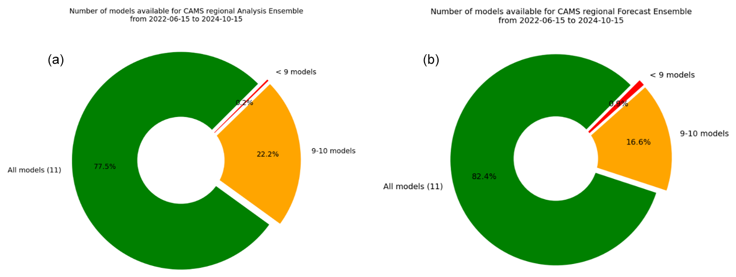
Figure 2 Distribution of the number of operational models having delivered on time to be included in the ENSEMBLE computation for the period 15 June 2022–15 October 2024: (a) NRT/AN (analysis) and (b) NRT/FC (forecasts).

Using the median to compute such an ensemble is a very robust approach to cope with potential missing members, and it has been shown to outperform individual models for average performances (Galmarini et al., 2004). It is however a very conservative approach, and developments are ongoing, in particular to improve the skills of the system to capture air quality exceedance detections by making use of machine-earning algorithms coupled to the raw CAMS Regional forecasts. Firstly, optimised forecasts at observation sites are produced operationally for four pollutants (PM₁₀, PM_2.5, NO₂ and O₃) at thousands of AQ e-reporting stations throughout Europe on a daily basis and for the 96 h forecast period. This product is referred to as CAMS-MOS (Model Output Statistics) (https://confluence.ecmwf.int/display/CKB/CAMS+Regional:+European+Air+Quality+Forecast+Optimised+at+Observation+Sites+data+documentation, last access: 22 September 2025). The underlying algorithm is a random forest using air pollutant concentration in the ENSEMBLE CTM as predictor as well as meteorological variables (temperature at 2 m, relative humidity, wind speed, and boundary layer height) (Bertrand et al., 2023). It is trained on a daily basis using the past 3 d of observations. As such, CAMS-MOS is a statistical model of the meteorological-dependent ENSEMBLE error, which proved very effective in improving the forecast skills in detecting exceedances of air quality information thresholds. Second, a weighted ensemble forecast at the same resolution as the CTMs (10 × 10 km²) has been developed. It consists of an optimum weighting of the 11 models calibrated on the past 7 d, but in this case the weights are constant and uniform and not dependent on meteorological predictors. CAMS-MOS is already available in the ADS as an operational product. But the weighted ensemble is still experimental. With the rapid development of machine learning and artificial intelligence, such experimental products will be further developed in the future.

4.2 Evaluation and Quality Control (EQC)

Evaluation and Quality Control is an essential part of CAMS in order to ensure the reliability and transparency of the products. For all the chemical species where a dense enough monitoring network allows a recurrent and statistically significant evaluation, synthetic performance reports are produced and made available on the CAMS website (https://atmosphere.copernicus.eu/regional-services, last access: 30 October 2024). These evaluations focus primarily on the surface in situ air quality regulatory monitoring networks for O₃, NO₂, PM₁₀, and PM_2.5. For the assimilated products, the evaluation is performed on about one-third of the stations, deliberately left out of the assimilation workflow (Sect. 2.3). The forecasts are evaluated using all available surface stations, whose spatial representativity ranges from rural to urban background air quality. The skill scores are updated at a daily frequency and available publicly through an interactive interface on the CAMS EQC pages for the ENSEMBLE and individual models. Quarterly summaries are produced in publicly available reports. They also include an evaluation of the models in the troposphere against above-surface measurements (aircraft and space-borne remote sensing and profiling). For the interim reanalysis and validated reanalysis, the evaluation reports are produced on an annual basis.

The present article is essentially a description of the system rather than a detailed analysis of its performance. Nevertheless, here we present several evaluation diagnostics for illustration purposes. Therefore, the performances of individual models contributing to the ENSEMBLE are anonymised as it would be too complex to provide the details of the performances of each model here that relate to intrinsic parameterisations. Such analysis is left for a dedicated future publication, but the interested user can also consult the interactive viewers and reference public reports on the Evaluation and Quality Control website to analyse the performances of individual models.

In Fig. 3 we show the root mean square error for surface ozone and PM₁₀ taken as the median over each quarter since the beginning of the CAMS production at the end of 2014 and over hundreds of European air quality monitoring stations. The figure is divided into two parts as urban background stations were only included in the evaluation as of autumn 2018 (note also that the vertical scales differ). It appears clearly that while the spread of the models was still substantial in the first part of the period, the system has reached a level of maturity since 2017, with more homogeneous performances between the various models and very few outliers. The ENSEMBLE model appears to give better scores overall. It can be surpassed in terms of RMSE in some occasions but not always by the same model, therefore still illustrating the added value of the multi-model ensemble approach. The range of performances today is about 12–18 µg m⁻³ for the RMSE (root mean square error) of daily maxima ozone, so the Key Performance Indicator of 18 µg m⁻³ is not always met depending on the models and the season. For PM₁₀, the RMSE is between 5 and 8 µg m⁻³, so the same KPI of 18 µg m⁻³ is usually met. Without entering into a more detailed analysis, it is visible that the scores are still gradually improving over the 2018–2023 period. In recent years, the median ENSEMBLE seems to have produced more systematically better performances and has become more difficult to beat.

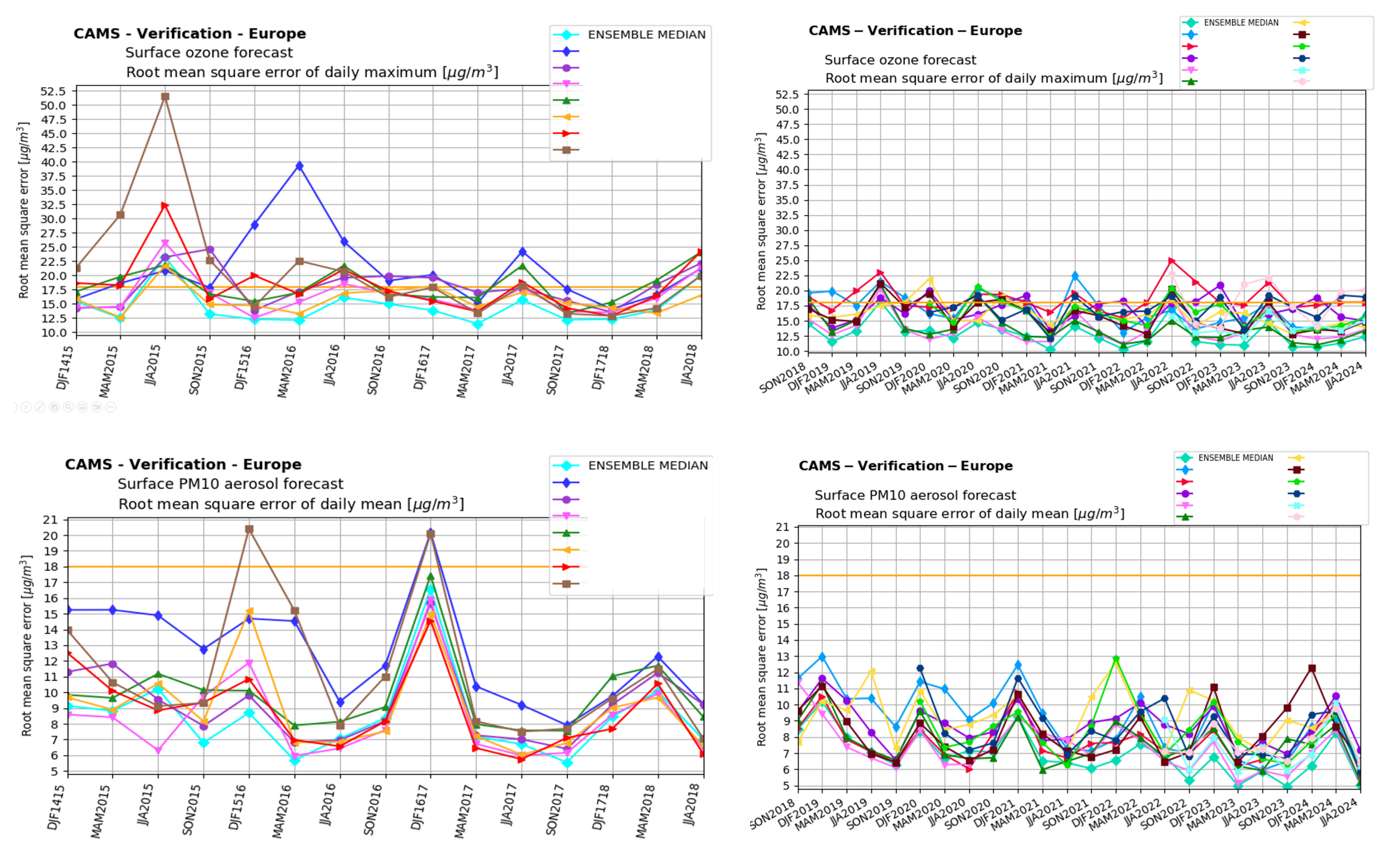
Figure 3 Evolution of the skill scores of the CAMS Regional Air Quality Forecasts (individual models and ENSEMBLE median) between 2014 and 2024 (divided into two parts: before and after 2018 as urban background stations were not included in the evaluation over the first period, and fewer models were available). Each point is the quarterly median of the RMSE (µg m⁻³) computed at regulatory air quality monitoring stations for the top, daily maximum ozone, and bottom, daily mean PM₁₀. The straight yellow line corresponds to the Key Performance Indicator for RMSE of 18 µg m⁻³.

In the European Air Quality regulation, detrimental air quality situations are identified in terms of various exceedance levels depending on the air pollutants. For PM₁₀, the daily mean concentrations should not exceed 50 µg m⁻³ more than 35 d (EC, 2008). The performance of the CAMS Regional reanalyses in capturing that threshold can be assessed through the performance diagram presented in Fig. 4. On the x axis the success ratio is the number of hits divided by the number of hits and false alarms. On the y axis, the probability of detection is the number of hits divided by the number of hits and misses. The dashed lines provide the frequency bias defined as the ratio of the total number of predicted exceedances to the total number of observed exceedances. For this example, for the year 2021, the ENSEMBLE median has the best success ratio, but some individual models outperform in terms of probability of detection. It is not possible to point out one single model which would outperform the ENSEMBLE systematically (the best-performing model will vary depending on the targeted pollutant, threshold, geographic area, etc.). Therefore, the reference product remains the median ENSEMBLE, which provides the best scores for conservative annual average metrics, but interested users can refer to the annual evaluation report to select alternative depending on their specific needs.

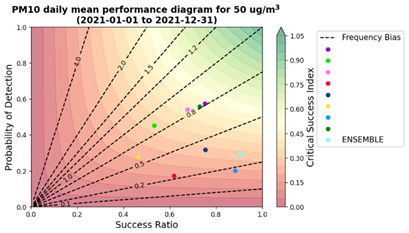
Figure 4 Performance of the CAMS Regional ENSEMBLE and individual models' reanalyses in capturing air quality threshold detection for daily mean PM₁₀ above 50 µg m⁻³ in 2021.

An illustration of the evaluation above the surface is provided in Fig. 5. The tropospheric column of NO₂ in the CAMS Regional ENSEMBLE forecast is compared to the observations from the TROPOMI instrument on board the Sentinel 5p satellite. The higher spatial resolution (approximately 5 km) available since the launch of the instrument allows urban-level NO₂ concentrations to be reached, therefore providing an excellent opportunity for the evaluation of spatial patterns of air pollution. Beyond surface and total columns, it is also essential to assess the performances of the vertical structure, as illustrated for the comparison with ozone soundings in Belgium (Uccle). Here both the regional forecast and analyses are compared to assess the impact of surface assimilation of air quality measurement on the vertical profiles. The CAMS global model forecast is also included along with the CAMS Regional ENSEMBLE range for the forecast and the analysis. A more detailed analysis of the comparison with satellite data can be found in Douros et al. (2023).

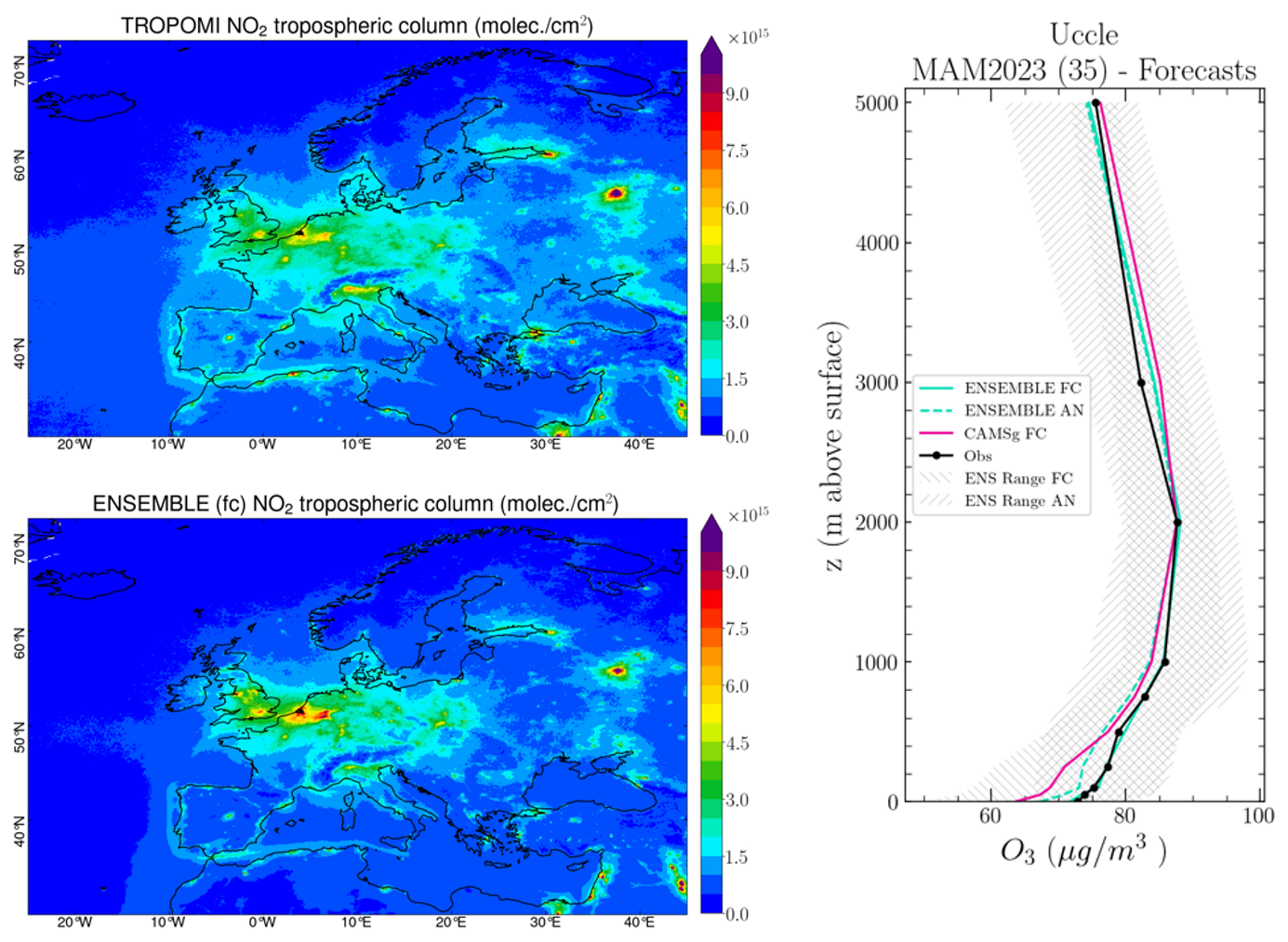
Figure 5 Left: evaluation over MAM-2023 of the CAMS Regional ensemble forecasts against TROPOMI satellite NO₂ tropospheric columns (10¹⁵ molec. cm⁻²). The CAMS NO₂ profiles have been multiplied with the TROPOMI kernels to remove the dependency on the retrieval a priori profile shape. Right: regional and global CAMS forecast and regional analyses of ozone compared to vertical profiles measured with ozone sondes over Uccle, Brussels, Belgium, for MAM 2023 (µg m⁻³). Source: CAMS2_83 Evaluation and Quality Control Service, https://atmosphere.copernicus.eu/regional-services (last access: 8 September 2025) (Gauss et al., 2023).

4.3 Dissemination and further use of the CAMS Regional Products

The results of the CAMS Regional Production System are made available publicly on the website at https://atmosphere.copernicus.eu/european-air-quality-forecast-plots (last access: 8 September 2025), where maps and time series of the various air pollutant and pollen species are displayed. The results of the median ENSEMBLE as well as each individual model are available for both forecast and analysis products with a 3-year retention time. Daily means, daily maxima, and hourly fields are available. The list of vertical levels available for interactive plotting on the website is surface, 100, 1000, 3000, and 5000 m (note that more vertical levels are available on the ADS). The model spread can also be assessed by selecting any grid point in the map to display the time series of the 4 d forecast including modelled dispersion, which provides information on the uncertainty in the ensemble forecast (Fig. 6).

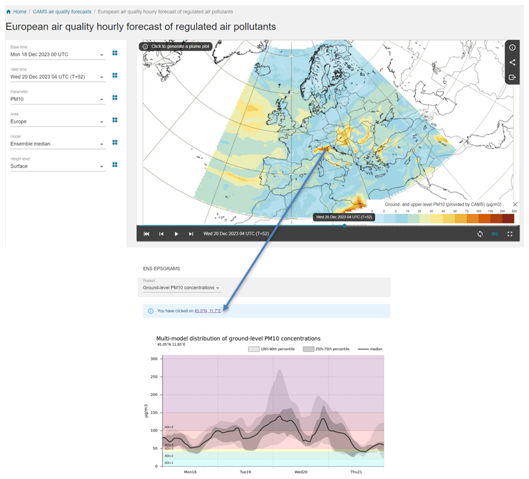
Figure 6 Screenshot of the CAMS Regional Production website displaying air quality forecasts over Europe (https://atmosphere.copernicus.eu, last access: 8 July 2025).

The Copernicus Atmosphere Data Store (ADS) constitutes an important dissemination pathway for the CAMS Regional Production System. All the numerical data can be freely retrieved through the website https://ads.atmosphere.copernicus.eu (last access: 8 September 2025), where automated requests can be built to download entire fields or custom extractions in either grib or netCDF formats.

The typical use of the CAMS Regional forecast product is for national and local air quality management agencies to understand the day-to-day air quality situation and anticipate major air pollution events. This can be done either by a qualitative analysis of quicklooks available on the CAMS website or through external companies that have developed alternative visualisation tools.

The numerical data obtained on the ADS can also be used as background information for national or local-scale air quality modelling applications. Such uses range from the nesting of a chemistry-transport model as three-dimensional and hourly concentrations of several chemical species are available in the CAMS Regional Forecast. They can also be used to feed Gaussian city-scale surface air quality models. There are also reported uses of the CAMS Regional Forecast to inform machine-learning air quality statistical prediction tools (Bertrand et al., 2023; Petetin et al., 2022).

The use of CAMS Regional reanalyses is rather to inform longer-term air quality applications. They can be used as background information for land-use regression models used in air quality policy products or exposure assessment for health impact studies (Horálek et al., 2022). They are also the primary source of information for the Interim Assessment Report produced annually by the CAMS Policy Service and serve as background information for European Member States in the Regulatory Air Quality reporting obligations (Hamer et al., 2023).

5 Conclusion and perspectives

The Regional Production System of the Copernicus Atmosphere Monitoring Service is today a well-established reference for air quality forecast and analysis in Europe and beyond. It is constituted of a unique ensemble of 11 European chemistry-transport models operated in 10 countries under the management of a Centralised Regional Production Unit. The system follows strict requirements in order to produce consistent air quality products through the ensemble of individual CTM. Those requirements include in particular forcing fields such as meteorology, chemical hemispheric boundary conditions, and surface fluxes of anthropogenic and wildfire emissions. But the added value of the use of an ensemble of models also lies in the diversity of the modelling strategy. As of today, the ensemble offers a very wide array of choices in terms of model design and structure, as well as regarding the formulation of underlying physical and chemical processes or forcing and coupling at the interfaces (land, sea, biosphere, etc.).

In the present paper, we provide comprehensive scientific documentation of the technical characteristics for the common forcing requirements as well as the diversity in modelling design brought about by the individual contributing modelling groups. We also explained how the billions of data produced on a daily basis are aggregated centrally, evaluated, and disseminated for a wide range of air quality applications. CAMS has been operational since the end of 2014 and has reached a high level of performance and stability today. Since 2017 the spread of model performances has converged, and it continues to improve gradually over the years.

As an operational service, the Regional Production of CAMS follows the research developments in the field of air quality modelling closely. A substantial part of the model development is undertaken independently by the modelling teams through various research projects and PhD work at a national level. International benchmarking activities (such as the AQMEII or Eurodelta initiatives, Galmarini et al., 2017; Colette et al., 2017) are also an important source of information to identify model development priorities. More recently, the European Union has launched a series of research projects devoted to the Evolution of Copernicus in the Horizon Europe Programme (https://atmosphere.copernicus.eu/copernicus-research-whats-horizon, last access: 8 September 2025).

In order to ensure a continuous improvement, the system follows a regular development cycle. The individual models are improved in time so that they remain in the state of the art of chemistry-transport modelling. When the progress becomes mature enough, system upgrades are scheduled on a bi-annual basis to allow individual modelling groups to bring their development into the operational model version. These bi-annual upgrades are also the opportunity to carry coordinated changes, such as the regular update of anthropogenic emission fluxes. Through these upgrades, the portfolio of products is also continuously expanding. For instance, in addition to the 19 chemical species already being delivered, the current plan at the time of submission of the present article (i.e. for the year 2024) is to include new PM species such as ammonium nitrate and a tracer of shipping emissions.

A large part of the research effort in relation to the Regional Production is related to chemistry-transport deterministic modelling. But there are also interesting prospects in the coupling between machine learning and physical and chemical modelling. The Regional Service already produces operationally optimised forecasts at station level on the basis of model output statistics which relies on machine learning to offer unprecedented performance in particular for air quality threshold detection (Bertrand et al., 2023). Novel methodologies to compute the ENSEMBLE model from the 11 individual production and move away from the conservative median approach are also under consideration.

Besides the modelling developments, the uptake of innovative observations is also instrumental in the long-term perspective of CAMS. The production of deposition fluxes is a good illustration of the need to make the best of available observations. While CTMs produce deposition fluxes by nature, they are not systematically quality-checked, and therefore the output products are limited at present to ambient air concentrations. A mid-term development is therefore ongoing to benchmark wet and dry deposition fluxes to ensure their robustness. To achieve this, CAMS relies on the network of deposition data collected in the EMEP network of rural supersites in Europe. But there are also promising prospects in the uptake of near-real-time advanced observations of atmospheric composition at the supersites of the ACTRIS European Research Infrastructure, in particular with regards to particulate matter chemical composition and source apportionment. Lastly, in the outlook of the future perspectives there are also high expectations regarding the uptake of geostationary satellite retrievals with the perspective of the launch of the Sentinel 4 satellite, which will bring unprecedented high-frequency atmospheric composition information over Europe.