NutGEnIE 1.0: nutrient cycle extensions to the cGEnIE Earth system model to examine the long-term influence of nutrients on oceanic primary production

Understanding the nuances of the effects of nutrient limitation on oceanic primary production has been the focus of many bioassay experiments by oceanographers. A theme of these investigations is that they identify the currently limiting nutrient at a given location, or in other words they identify the proximate limiting nutrient (PLN). However, the ultimate limiting nutrient (ULN; the nutrient whose supply controls system productivity over extensive timescales) can be different from the PLN. Our motivation is to investigate the identity of the ULN. The ULN constrains oceanic primary production over extensive timescales and consequently overall ocean fertility. The rate of oceanic photosynthesis affects planetary oxygen and carbon dioxide, impacting climate. Understanding past ocean fertility is fundamental to understanding Earth system history and biological evolution.

Investigations that have considered the ULN have often utilised box models for example the work of, Tyrrell (1999) and Lenton and Watson (2000). To facilitate investigation of the ULN the carbon-centric Grid Enabled Integrated Earth system model (cGEnIE) nutrient cycles have been extended to create NutGEnIE. NutGEnIE incorporates three open nutrients cycles nitrogen, phosphorus, and iron. The impacts of diazotrophs, capable of fixing nitrogen, are represented alongside those of other phytoplankton. NutGEnIE is capable of extended duration model simulations necessary to investigate the ULN while, at the same time, including iron as a potentially limiting nutrient. NutGEnIE is described here, with particular focus on the biogeochemical cycles of iron, nitrogen and phosphorus. Model results are compared to ocean observational data to assess the degree of realism. Model-data comparisons include physical properties, nutrient concentrations, and process rates (e.g., export and nitrogen fixation). The comparisons of NutGEnIE to ocean observational data are largely positive, suggesting that the dynamics of NutGEnIE are valid. The validations, allied to the ability to run an Earth System model with open nutrients cycles of nitrogen, phosphorus, and iron over extensive time periods supports the proposed use of NutGEnIE to revisit the question of the ULN for oceanic primary production.

1 Introduction

1.1 The importance of oceanic primary production

Photosynthetic phytoplankton that inhabit the sunlit ocean surface, the euphotic zone, are responsible for the majority of ocean primary production (PP) and form the base of marine food webs. These photosynthetic phytoplankton, photoautotrophs, use light to fix dissolved carbon dioxide (CO₂) and other nutrients into biomass that fuels the pelagic ecosystem, and ultimately leads to the export of carbon to depth via a process known as the biological carbon pump (BCP) (Chisholm, 2000; Boyd et al., 2019). The strength of the BCP can influence atmospheric concentrations of CO₂ and therefore Earth's carbon cycle and climate (Sarmiento et al., 1998; Hain et al., 2014; Galbraith and Skinner, 2020). Net primary production (NPP) represents the total rate of organic carbon production minus the rate of respiration by phytoplankton; it therefore represents the rate that phytoplankton produce biomass (Sigman and Hain, 2012). Estimates of global marine NPP based on satellite, float or ecosystem models are ∼50–60 Pg C yr⁻¹ (petagrams of carbon per year) (Carr et al., 2006; Silsbe et al., 2016; Johnson and Bif, 2021). Ocean uptake of CO₂, mostly through abiotic processes, has contributed to mitigating much of the impact of anthropogenic CO₂ emissions with approximately half taken up by a combination of land and ocean carbon reservoirs (Ballantyne et al., 2012; Friedlingstein et al., 2022). Understanding of the controls on ocean NPP levels can provide insights into Earth's past, current and potential future carbon cycle. Nutrient supply to the euphotic zone acts as a fundamental control on ocean PP levels; this supply and subsequent growth limitation are the focus of the model extensions we present here.

1.2 Factors limiting primary production

Predation or grazing from higher trophic levels can be categorised as “top-down” control of phytoplankton PP; by reducing phytoplankton populations, consequently reducing the total amount of photosynthesis. When not at optimal levels, light, temperature, and nutrients cause realised growth rates to be below the maximum growth rate of a phytoplankton population and can be considered as “bottom-up” controls on PP. Light as a source of energy is an obvious potential limitation to photosynthetic phytoplankton. The nature of light limitation has been considered and methods of modelling it developed (e.g. Marra et al., 1985; Yang et al., 2020). Temperature also regulates biological rates as individual species have a relatively narrow optimal temperature range with growth declining rapidly outside this range (Gillooly et al., 2002). When community production is considered, growth rates increase exponentially with temperature as species with higher optimal growth ranges are favoured (Eppley, 1972); furthermore, studies have proposed methods of modelling temperature limitation (e.g. Grimaud et al., 2017; O'Donnell et al., 2018).

Elements obtained from nutrients are essential components of macro-molecules such as proteins and nucleic acids (Moore et al., 2013). Nutrient limitation is a condition or state where addition of a nutrient would stimulate growth (Cullen, 1991; de Baar, 1994). Addition of the proximate limiting nutrient (PLN) stimulates immediate growth, whereas addition of the ultimate limiting nutrient (ULN) enhances total system productivity over extensive timescales (Cullen, 1991; Tyrrell, 1999).

Much work has been conducted to describe the nature of phytoplankton nutrient requirements (Redfield, 1934, 1958) and subsequent limitation of growth (Sommer, 1986; Timmermans et al., 2004; Flynn, 2010; Bestion et al., 2018). Moore et al. (2013) and Browning and Moore (2023) conducted extensive analysis to compare nutrient availability to phytoplankton nutrient requirements. This work enabled the determination of spatial variations of proximate nutrient limitations. Further analysis linked nutrient deficiencies to large-scale ocean physical–chemical–biological processes (Moore, 2016).

Oceanographers have conducted numerous experiments to investigate nutrient limitation of oceanic PP. A great deal of this work has involved the use of bioassay experiments that consist of the addition of nutrients to samples of surface ocean water to determine which stimulates the greatest phytoplankton growth (Mills et al., 2004; Bonnet et al., 2008; Moore et al., 2008). The concept of iron fertilisation also gained focus following the work of Martin (1990), prompting a range of iron fertilisation experiments. These experiments involved in situ iron fertilisation (Martin et al., 1994; Boyd and Abraham, 2001; Hoffmann et al., 2006) – in effect field bioassay experiments. The implications of many bioassay and fertilisation experiments was summarised and synthesised by Moore et al. (2013), who were able to identify primary, secondary, and co-limiting nutrients across many regions. Moore (2016) compared the stoichiometry of the elemental requirements of phytoplankton to the elemental composition of ocean basins' deep water, that acts to supply nutrients to surface water. Browning and Moore (2023) conducted further synthesis of over 150 bioassay and fertilisation experiments, identifying three dominant nutrient limitation regimes. Their work suggest the stratified subtropical gyres and summertime Arctic Ocean are nitrogen limited, upwelling regions are typically iron limited and remaining regions are most commonly co-limited by iron and nitrogen (Browning and Moore, 2023). The underlying bioassay experiments and analysis mentioned here have a common theme in that they focus on the immediate nutrient deficiency situation in a temporal sense, and often focus on a specific ocean location. This focus on the immediate nutrient deficiency identifies the PLN.

Tyrrell (1999) used a box model approach to identify nitrate as the PLN and phosphate as the ULN. In contrast, Falkowski (1997) argued that the dynamics of the nitrogen cycle, with particular emphasis on the limiting role iron has on nitrogen fixation, has ultimate control over phytoplankton productivity. Deutsch et al. (2007) concluded that nitrogen fixation stabilises the oceanic fixed nitrogen inventory over time but that water column denitrification rather than atmospheric inputs of iron determine nitrogen fixation rates. Moore and Doney (2007) concluded that for much of the global ocean iron is the ultimate limiting nutrient. There were some shortcomings in prior work to identify the ULN: (a) Tyrrell (1999) did not include iron, consequently the high iron requirements of the enzyme nitrogenase central to nitrogen fixation were not captured; (b) Falkowski (1997) provided an analysis based on the evolution of biogeochemical cycles, without supporting the analysis with modelling; (c) Deutsch et al. (2007) only conducted model simulations over short timescales to a modern ocean steady-state; and (d) Moore and Doney (2007) focused primarily on the nutrient regime of the Southern Ocean.

These shortcomings and other considerations suggest the desirability of a new modelling approach to the ULN question in which the model used possesses the following characteristics: (1) cycling and biological uptake of (and potential limitation by) all three nutrients (N, P, Fe), (2) nitrogen-fixing as well as non-fixing phytoplankton, (3) spatial resolution, as opposed, for instance, to representing the whole surface ocean with one box, (4) the ability to carry out model runs exceeding the residence times of all three nutrients, and (5) external inputs (e.g. delivery of nutrients down rivers) and external outputs (e.g. delivery of nutrients to seafloor sediments via burial) in an “open” model allowing total ocean inventories of nutrients to change over time.

1.3 Investigating the ultimate limiting nutrient

Investigations that have considered ULN have often utilised box models for example the work of, Tyrrell (1999) and Lenton and Watson (2000). Here we propose to establish a model approach that can be used subsequently to study the long-term influence of nutrients on PP and diagnose the ULN. Such investigations will require full ocean investigations to be executed over tens of thousands of years, given the long residence times of nutrients in the global ocean. Delaney (1998) indicate phosphorus has a residence time of several tens of thousands of years, nitrogen has a residence time of a few thousand years (Gruber, 2004) and iron a residence time of tens to hundreds of years (Hayes et al., 2018). For that to be successful the carbon-centric Grid Enabled Integrated Earth system model (cGEnIE) has been configured and modified to include three open nutrient cycles for nitrate, phosphate, and iron (Sect. 2) to create a variant referred to hereafter as nutrient-centric Grid Enabled Integrated Earth system model (NutGEnIE).

A background overview of the cGEnIE model framework is provided in Sect. 2.1 and 2.2, followed by a more detailed descriptions of the aspects of NutGEnIE nutrient cycles that have been configured to support the ongoing analysis. Details of the validation approach (Sect. 3.1) and subsequent results (Sect. 3.2 and 3.3) and discussion follow.

2 Model description

2.1 Physical model of cGEnIE

The ocean physics and climate model in cGEnIE are based on the fast climate model “C-GOLDSTEIN” of Edwards and Marsh (2005). C-GOLDSTEIN is comprised of a reduced physics (frictional geostrophic) 3-D ocean circulation model coupled to a 2-D energy–moisture balance model (EMBM) and a dynamic–thermodynamic sea ice model (Edwards and Marsh, 2005; Marsh et al., 2011). The ocean model calculates the horizontal and vertical transport of heat, salinity, and biogeochemical tracers using a parameterisation for isoneutral diffusion and eddy-induced advection (Edwards and Marsh, 2005; Marsh et al., 2011). The ocean model additionally determines heat and moisture exchanges with the atmosphere, sea ice, and land, and is forced at the ocean surface by zonal and meridional wind stress according to a specified wind field. Horizontal transport of sea ice is resolved by the sea ice model in addition to the exchange of heat and fresh water with the ocean and atmosphere. A full description of the C-GOLDSTEIN model can be found in Edwards and Marsh (2005) and, with updates, in Marsh et al. (2011).

The ocean model is configured on a 36×36 equal-area horizontal grid. The grid is uniform in longitude (10° increments) and uniform in the sine of latitude (resulting in latitude increments of approximately 3.2° at the Equator increasing to 19.2° at the highest latitude). The ocean has 16 logarithmically spaced z-coordinate levels in the vertical. The thickness of the vertical levels increases with depth, from 80.8 m at the surface to 765 m at the deepest level. The configured representation of the grid and bathymetry is shown in Fig. 1. C-GOLDSTEIN is run with 96 time steps per year and is configured based on the parameterisation detailed in the fifth row (GENIE-16) of Table 1 of Cao et al. (2009).

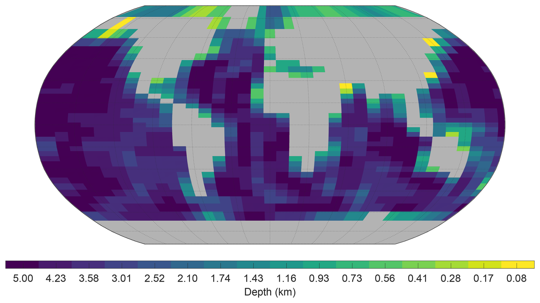
Figure 1 The modern cGEnIE gridded continental configuration and ocean bathymetry (depth in km). Based on 16 depth levels and a 36×36 equal area grid of cGEnIE. Exact depths at the bottom of each depth level are provided in Table S1.

2.2 Biogeochemistry framework (BioGEM)

cGEnIE includes a series of geochemical tracers within the biogeochemical model component referred to as BIOGEM (Ridgwell et al., 2007). The biological part of BIOGEM is abstracted relative to reality and does not maintain explicit biomass tracers (such as phytoplankton concentrations) for ocean life (Ridgwell et al., 2007). Biological activity is estimated from surface nutrient uptake which in turn is immediately converted to particulate and dissolved organic matter (POM and DOM) in the surface ocean (Ridgwell et al., 2007). The subsequent processing associated with POM and DOM is discussed in detail in Sect. 2.3. This abstracted approach results in a computationally efficient model that represents biogenically-induced chemical fluxes (Maier-Reimer, 1993) and is capable of execution timescales required to investigate the ULN. The basis of the biological nutrient uptake and export scheme is similar to that of Parekh et al. (2005). This has in turn been developed subsequently by work of others including Monteiro et al. (2012) and Reinhard et al. (2020).

Three tracer categories (atmospheric, oceanic, and sedimentary) track biogeochemical processes within the cGEnIE model. Atmospheric tracers include carbon dioxide and oxygen. A more extensive range of ocean tracers are used: dissolved inorganic carbon (DIC) and dissolved oxygen; nitrate (NO${}_{\mathrm{3}}^{-}$) and ammonium (NH${}_{\mathrm{4}}^{+}$) as forms of fixed nitrogen or dissolved inorganic nitrogen (DIN); phosphate (PO${}_{\mathrm{4}}^{\mathrm{3}-}$); iron (Fe); dissolved organic matter, partitioned between carbon (DOC), nitrogen (DON), phosphorus (DOP), and iron (DOFe); tracers associated with the iron cycle to track ligands and complexed ligand-bound iron; and additional tracers that include dissolved dinitrogen (N₂), calcium (Ca) and sulphate (SO${}_{\mathrm{4}}^{\mathrm{2}-}$). Ocean tracers for POM are not used as POM is immediately remineralised following the scheme set out in Sect. 2.3.7. Sedimentary tracers include POM (partitioned by nutrient), calcium carbonate and detrital material. By default, results are output as annual averages, however the BIOGEM module computes tracers at 48 time steps per year allowing the possibility of results relating to shorter timeframes.

2.3 Biogeochemistry extensions (NutGEnIE)

The focus of this section is to describe the nutrient cycles and utilisation of those nutrients by PP; a full list of ocean tracers enabled in the NutGEnIE configuration is provided in provided in Table S2. NutGEnIE is an extension to the BioGEM module within cGEnIE. The novel features of the configuration of NutGEnIE described here includes (a) the concurrent use of three open nutrient (N, P and Fe) cycles when determining phytoplankton growth (surface nutrient uptake) and (b) the representation of a second iron binding ligand class with stronger binding in the upper water column. The three nutrients N, P and Fe have been included in previous versions of cGEnIE (Monteiro et al., 2012; Naafs et al., 2019) but without the surface and seafloor input fluxes introduced here and with uniform ligand binding within the iron cycle. In this section we detail the most pertinent features of BioGEM alongside the extensions made in NutGEnIE.

NutGEnIE does not maintain the biomass of phytoplankton or model grazing by zooplankton; it utilises the limiting nutrient concentration within cells to calculate the rate of creation of new phytoplankton. The nutrient uptake processes differ for the two classes of phytoplankton considered within the model. Diazotrophs (designated by the superscript Diaz) are those phytoplankton capable of nitrogen fixation. The other phytoplankton class (designated by the superscript OPhy) are not capable of nitrogen fixation and must source nitrogen from the DIN in the surface waters. Nutrient uptake by other phytoplankton (Γ^OPhy) is described in Sect. 2.3.1; similarly, nutrient uptake by diazotrophs (Γ^Diaz) is described in Sect. 2.3.2. The nutrient uptake terms (Γ^OPhy and Γ^Diaz) are calculated in the surface layer.

In NutGEnIE, nutrients taken up by phytoplankton are instantly converted to POM and DOM in the surface ocean. The ratio of POM to DOM is set by a configuration option calibrated against nutrient observations as described in Ridgwell et al. (2007). POM is subject to immediate gravitational sinking to the ocean interior, without lateral advection, where it is immediately remineralised. DOM (maintained as a tracer for each nutrient DOM_C, DOM_N, DOM_P and DOM_Fe) is subject to ocean circulation and mostly retained in the surface ocean. DOM has an assumed lifetime governed by a degradation rate constant (λ, 0.5 yr⁻¹) with remineralisation occurring as outlined in Sect. 2.3.7 (Reinhard et al., 2020).

We intend to use the model to investigate the ULN and for this purpose it is essential that nutrient cycles are open. Therefore, in NutGEnIE a removal (burial) flux is applied by removing a fixed proportion (k_BF) of nutrient uptake by other phytoplankton and diazotrophs from the modelled ocean. This represents a simplified instantaneous sediment burial term that is not coupled to POM remineralisation dynamics. External inputs are also applied, via rivers and/or the atmosphere and seafloor.

Table 1 Biogeochemical parameters of NutGEnIE relating to nutrient tracers. These parameters relate to Eqs. (1)–(2), (5)–(11), (13)–(15). Where the model value of the parameter differs from the literature reference value, the literature value is provided.

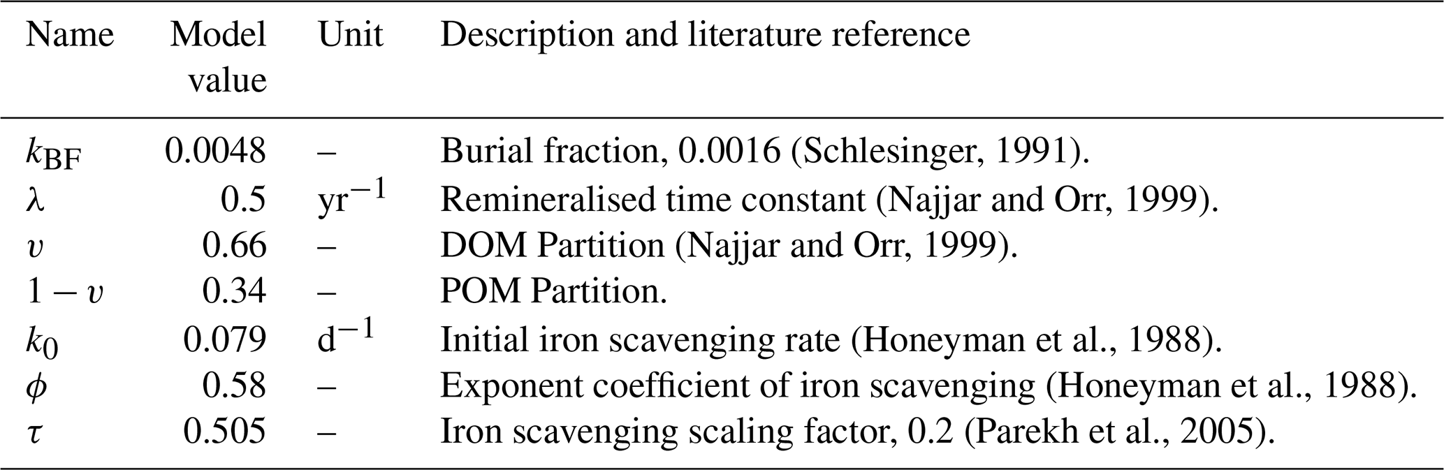
The portion of nutrient uptake; (Γ^NOPhy and Γ^NDiaz for other phytoplankton and diazotrophs respectively); that is available for remineralisation is determined after the subtraction of the burial removal flux (k_BF), see Eqs. (1) and (2). Within each surface cell a proportion (k_BF) of the nutrient uptake in that cell is lost and made unavailable for remineralisation. Setting k_BF to a value of zero would negate this removal flux mechanism. The values, units and brief description of equation constants are provided in Table 1.

$$\begin{array}{}\text{(1)}& {\displaystyle }& {\displaystyle }{\mathrm{\Gamma }}^{\mathrm{NOPhy}}=\left(\mathrm{1}-k_{\mathrm{BF}}\right){\mathrm{\Gamma }}^{\mathrm{OPhy}}\text{(2)}& {\displaystyle }& {\displaystyle }{\mathrm{\Gamma }}^{\mathrm{NDiaz}}=\left(\mathrm{1}-k_{\mathrm{BF}}\right){\mathrm{\Gamma }}^{\mathrm{Diaz}}\end{array}$$

The understanding of the oceanic iron cycle has developed in recent years; a comprehensive summary is provided in Fig. 2 of Tagliabue et al. (2017). Tagliabue et al. (2017) identify aeolian dust deposition, rivers, sea-ice, hydrothermal systems and sediments as sources of iron. The iron cycle of NutGEnIE has been extended so that it includes surface dust deposition, a surface flux that represents riverine inputs and a benthic flux to represent hydrothermal systems and sediments as sources of iron.

Nitrogen cycling within NutGEnIE represents the various forms of nitrogen; that is, nitrate, ammonium, dinitrogen, and organic nitrogen. The cycling is achieved by the processes of uptake of nitrate and ammonium by other phytoplankton, nitrogen fixation by diazotrophs, denitrification, and nitrification (Monteiro et al., 2012). However, in reality in oxygen minimum zones additional removal pathways exist, for instance dissimilatory nitrate reduction to ammonia and anaerobic ammonium oxidation (anammox) (Lam et al., 2009). Like denitrification, anammox converts DIN to N₂, i.e. reducing the inventory of DIN (Lam et al., 2009). Because of their similar biogeochemical consequences, and because both only occur in low oxygen conditions, anammox is not represented as a separate process. Denitrification is solely based on organic matter remineralisation.

The structures of the phosphorus, DIN and iron cycles in NutGEnIE are shown in Fig. 2. Input and output fluxes associated with each nutrient are shown alongside the primary processes that influence nutrient concentrations. Each nutrient cycle is discussed in more detail in the following sections. The spatial distribution of input fluxes surface PO${}_{\mathrm{4}}^{\mathrm{3}-}$ ($S_{{\mathrm{PO}}_{\mathrm{4}}}$), surface NO${}_{\mathrm{3}}^{-}$ ($S_{{\mathrm{NO}}_{\mathrm{3}}}$), dust deposition of iron (DD_Fe) and seafloor flux of iron (B_Fe) are shown in Figs. S1–S3 in the Supplement.

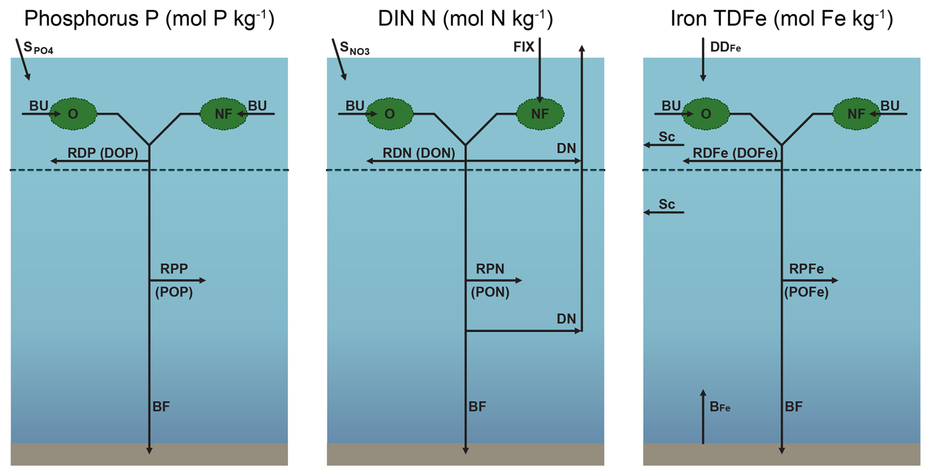
Figure 2 Structure of NutGEnIE nutrient cycles. DIN, dissolved inorganic nitrogen (DIN = NO${}_{\mathrm{3}}^{-}$ + NH${}_{\mathrm{4}}^{+}$). TDFe, total dissolved iron. BU, biological uptake of nutrients by O, other phytoplankton and NF, nitrogen fixers (diazotrophs) occurs in the surface ocean layer. Surface inputs ($S_{{\mathrm{PO}}_{\mathrm{4}}}$ and $S_{{\mathrm{NO}}_{\mathrm{3}}}$) and dust deposition of iron (DDFe) are input fluxes to the surface ocean; BFe, seafloor flux of iron; FIX, nitrogen fixation; DN, denitrification; Sc, scavenging of iron; BF, burial fraction; RDP, RDN and RDFe are remineralisation of dissolved organic phosphate (DOP), nitrate (DON) and iron (DOFe) respectively. RPP, RPN and RPFe are remineralisation of particulate organic phosphate (POP), nitrate (PON) and iron (POFe) respectively. Remineralisation of dissolved and particulate organic matter occurs throughout the water column.

2.3.1 Other phytoplankton nutrient uptake

Primary production (PP) is accounted for via the production of organic matter resulting from the uptake of nutrients. The nutrient framework is configurable, with an option to include silicon, but in NutGEnIE it is made to be dependent on DIN (= NO${}_{\mathrm{3}}^{-}$ + NH${}_{\mathrm{4}}^{+}$), PO${}_{\mathrm{4}}^{\mathrm{3}-}$ and Fe_T (= Fe^′ + FeL). Fe_T is the total bioavailable iron, which is discussed, along with the processes of iron complexation, in Sect. 2.3.6. Nutrient uptake by non-diazotrophs (other phytoplankton) results in the production of organic matter (Γ^OPhy) at a rate subject to Eq. (3) (Monteiro et al., 2012).

$$\begin{array}{}\text{(3)}& \begin{array}{rl}{\mathrm{\Gamma }}^{\mathrm{OPhy}}=& V_{\max }^{\mathrm{OPhy}}\left(\mathrm{1}-f_{\mathrm{ice}}\right){\mathit{\gamma }}^T{\mathit{\gamma }}^I\\ & \min \left[{\displaystyle \frac{{\mathrm{PO}}_{\mathrm{4}}^{\mathrm{3}-}}{{\mathrm{PO}}_{\mathrm{4}}^{\mathrm{3}-}+K_{\mathrm{P}}}};{\displaystyle \frac{\mathrm{DIN}}{\mathrm{DIN}+K_{\mathrm{N}}}};{\displaystyle \frac{F{e}_{\mathrm{T}}}{F{e}_{\mathrm{T}}+K_{\mathrm{Fe}}}}\right]\\ & \min \left[{\mathrm{PO}}_{\mathrm{4}}^{\mathrm{3}-};{\displaystyle \frac{\mathrm{DIN}}{R_{\mathrm{N}}^{\mathrm{OPhy}}}};{\displaystyle \frac{F{e}_{\mathrm{T}}}{R_{\mathrm{Fe}}^{\mathrm{OPhy}}}}\right]\end{array}\end{array}$$

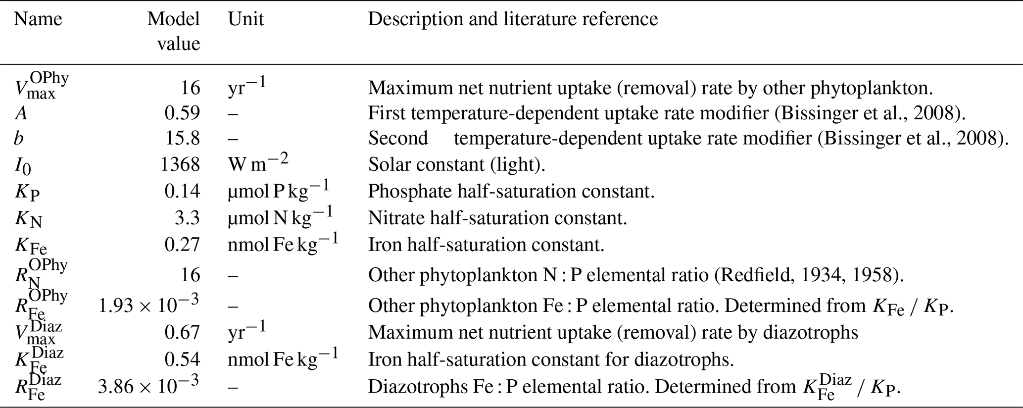
Nutrient limitation follows a Michaelis–Menten approach with a minimum law of nutrients. K_P, K_N, and K_Fe are the other phytoplankton half-saturation constants for phosphate, DIN, and iron, respectively. The concentration of the limiting nutrient therefore determines the other phytoplankton biomass, an approach that is often adopted in biogeochemical modelling (Maier-Reimer, 1993; Doney et al., 2006; Monteiro et al., 2012). $V_{\max }^{\mathrm{OPhy}}$ is the maximum net nutrient uptake rate of other phytoplankton. The term (1−f_ice) ensures nutrient uptake is restricted to ice free locations as f_ice is the fraction of ice-covered surface ocean. A temperature limitation term γ^T is based on an Eppley curve. ${\mathit{\gamma }}^T=A{e}^{T/b}$, where T is the temperature (°C) and A and b the associated Eppley constants (Eppley, 1972; Bissinger et al., 2008). Light limitation is represented by γ^I, ${\mathit{\gamma }}^I=I/I_{\mathrm{0}}$, where I is the amount of light and I₀ the solar constant (Monteiro et al., 2012). The uptake by other phytoplankton is in units of phosphorus. Therefore, DIN and Fe_T uptake are scaled by the other phytoplankton elemental composition ($R_{\mathrm{N}}^{\mathrm{OPhy}}=\mathrm{N}:\mathrm{P}$ and $R_{\mathrm{Fe}}^{\mathrm{OPhy}}={\mathrm{Fe}}_{\mathrm{T}}:\mathrm{P}$). The values, units and brief description of equation constants are provided in Table 2.

Table 2 Biogeochemical parameters of NutGEnIE relating to nutrient uptake. These parameters relate to Eqs. (3) and (4). Where the model value of the parameter differs from the literature reference value, the literature value is provided.

2.3.2 Nitrogen fixation and diazotrophs nutrient uptake

The activity of diazotrophs in NutGEnIE is also accounted for by the production of organic matter resulting from the uptake of nutrients. The availability of N₂ supplied via atmospheric transfer is deemed to be unlimited so that the production of organic matter (Γ^Diaz) is at a rate subject to Eq. (4) (Monteiro et al., 2012).

$$\begin{array}{}\text{(4)}& \begin{array}{rl}{\mathrm{\Gamma }}^{\mathrm{Diaz}}=& V_{\max }^{\mathrm{Diaz}}\left(\mathrm{1}-f_{\mathrm{ice}}\right){\mathit{\gamma }}^T{\mathit{\gamma }}^I\\ & \min \left[{\displaystyle \frac{{\mathrm{PO}}_{\mathrm{4}}^{\mathrm{3}-}}{{\mathrm{PO}}_{\mathrm{4}}^{\mathrm{3}-}+K_{\mathrm{P}}}};{\displaystyle \frac{F{e}_{\mathrm{T}}}{F{e}_{\mathrm{T}}+K_{\mathrm{Fe}}^{\mathrm{Diaz}}}}\right]\\ & \min \left[{\mathrm{PO}}_{\mathrm{4}}^{\mathrm{3}-};{\displaystyle \frac{{\mathrm{Fe}}_{\mathrm{T}}}{R_{\mathrm{Fe}}^{\mathrm{Diaz}}}}\right]\end{array}\end{array}$$

But this holds only if $\frac{\mathrm{DIN}}{R_{\mathrm{N}}^{\mathrm{OPhy}}}<\min \left[{\mathrm{PO}}_{\mathrm{4}}^{\mathrm{3}-};\frac{\mathrm{Fe}}{R_{\mathrm{Fe}}^{\mathrm{OPhy}}}\right]$ and DIN<N_thresh, otherwise the rate is zero. Together these two conditions only allow nitrogen fixation if DIN is scarce and if it is the limiting nutrient for other phytoplankton.

$V_{\max }^{\mathrm{Diaz}}$ is the maximum net nutrient uptake of diazotrophs and is assumed to be lower than $V_{\max }^{\mathrm{OPhy}}$ because of the energy demands of the process of N₂ fixation. The ice fraction, temperature and light limitation aspects are the same as for other phytoplankton (Eq. 3 above). A higher Fe requirement for diazotrophs is consistent with the iron demands of the nitrogenase enzyme (Berman-Frank et al., 2007). The values, units and brief description of equation constants are provided in Table 2. Oligotrophic environments are defined as having DIN<N_thresh (Monteiro et al., 2012). For the modern ocean a threshold can be constrained by observations leading to a fixed threshold N_thresh≈2 µmol DIN L⁻¹ (Monteiro et al., 2011).

2.3.3 Phosphorus cycle and update

Here we cover the main governing equations in NutGEnIE. For each nutrient an equation is provided for it, alongside an equation for its dissolved organic matter, e.g., for phosphorus the equations for phosphate and DOP are provided. These equations represent the mechanism employed in NutGEnIE to maintain the tracer concentrations throughout the water column. Note that the transport terms calculated by the ocean circulation model (Edwards and Marsh, 2005) are omitted.

$$\begin{array}{}\text{(5)}& {\displaystyle }& {\displaystyle \frac{\partial {\mathrm{PO}}_{\mathrm{4}}^{\mathrm{3}-}}{\partial t}}=-{\mathrm{\Gamma }}_{\mathrm{P}}^{\mathrm{OPhy}}-{\mathrm{\Gamma }}_{\mathrm{P}}^{\mathrm{Diaz}}+\mathit{\lambda }\mathrm{DO}P+S_{{\mathrm{PO}}_{\mathrm{4}}}\text{(6)}& {\displaystyle }& {\displaystyle \frac{\partial \mathrm{DOP}}{\partial t}}=v\left({\mathrm{\Gamma }}_{\mathrm{P}}^{\mathrm{NOPhy}}+{\mathrm{\Gamma }}_{\mathrm{P}}^{\mathrm{NDiaz}}\right)-\mathit{\lambda }\mathrm{DOP}\end{array}$$

${\mathrm{\Gamma }}_{\mathrm{P}}^{\mathrm{OPhy}}$ is the biological uptake of PO${}_{\mathrm{4}}^{\mathrm{3}-}$ by other phytoplankton as described in Sect. 2.3.1. Similarly, ${\mathrm{\Gamma }}_{\mathrm{P}}^{\mathrm{Diaz}}$ is the biological uptake of PO${}_{\mathrm{4}}^{\mathrm{3}-}$ by diazotrophs described in Sect. 2.3.2. A proportion (v) of the nutrients taken up by diazotrophs and other phytoplankton is partitioned into DOM. This DOM is subsequently remineralised with a time constant (λ). The remaining proportion (1−v) of the nutrient uptake is partitioned into POM that undergoes water column remineralisation as detailed in Sect. 2.3.7. The values of v and λ, are configurable, but in NutGEnIE are given default values of v=0.66 and λ=0.5 yr⁻¹ following the OCMIP-2 protocol (Najjar and Orr, 1999). The values, units and brief description of equation constants are provided in Table 1.

$S_{{\mathrm{PO}}_{\mathrm{4}}}$ represents a surface input flux of PO${}_{\mathrm{4}}^{\mathrm{3}-}$ such as riverine inputs. The magnitude of this flux is configurable via a parameter that defines the annual moles of PO${}_{\mathrm{4}}^{\mathrm{3}-}$ added. The $S_{{\mathrm{PO}}_{\mathrm{4}}}$ flux is distributed evenly to cells adjacent to land (excluding Antarctica); all other cells, do not receive the input flux, see Fig. S1. The novel aspects of the phosphorus cycle in NutGEnIE are that it is open with a input flux $S_{{\mathrm{PO}}_{\mathrm{4}}}$ and removal flux mechanism (Eqs. 1 and 2) allowing the phosphorus inventory to adjust. The input flux $S_{{\mathrm{PO}}_{\mathrm{4}}}$ can be adjusted, as required for the future work to investigate the ULN.

2.3.4 Nitrogen cycle and update

Nutrient uptake by other phytoplankton is dependent on the availability of DIN, i.e., the combination of NO${}_{\mathrm{3}}^{-}$ and NH${}_{\mathrm{4}}^{+}$ concentrations. The uptake rates of NO${}_{\mathrm{3}}^{-}$ and NH${}_{\mathrm{4}}^{+}$ are represented by Eqs. (7) and (8) with NH${}_{\mathrm{4}}^{+}$ being preferentially utilised (Naafs et al., 2019).

$$\begin{array}{}\text{(7)}& {\displaystyle }& {\displaystyle }{\mathrm{Up}}_{{\mathrm{NH}}_{\mathrm{4}}}=\min \left({\mathrm{\Gamma }}_{\mathrm{N}}^{\mathrm{OPhy}};{\mathrm{NH}}_{\mathrm{4}}^{+}\right)\text{(8)}& {\displaystyle }& {\displaystyle }{\mathrm{Up}}_{{\mathrm{NO}}_{\mathrm{3}}}={\mathrm{\Gamma }}_{\mathrm{N}}^{\mathrm{OPhy}}-{\mathrm{Up}}_{{\mathrm{NH}}_{\mathrm{4}}}\end{array}$$

The governing equations for NH${}_{\mathrm{4}}^{+}$ and NO${}_{\mathrm{3}}^{-}$ are below.

$$\begin{array}{}\text{(9)}& {\displaystyle }& {\displaystyle \frac{\partial {\mathrm{NH}}_{\mathrm{4}}^{+}}{\partial t}}=-{\mathrm{Up}}_{{\mathrm{NH}}_{\mathrm{4}}}-{\mathrm{O}}_{\mathrm{Nit}}+\mathit{\lambda }\mathrm{DON}\text{(10)}& {\displaystyle }& {\displaystyle \frac{\partial {\mathrm{NO}}_{\mathrm{3}}^{-}}{\partial t}}=-{\mathrm{Up}}_{{\mathrm{NO}}_{\mathrm{3}}}+{\mathrm{O}}_{\mathrm{Nit}}-R_{{\mathrm{NO}}_{\mathrm{3}}}+S_{{\mathrm{NO}}_{\mathrm{3}}}\text{(11)}& {\displaystyle }& {\displaystyle \frac{\partial \mathrm{DON}}{\partial t}}=v\left({\mathrm{\Gamma }}_{\mathrm{N}}^{\mathrm{NOPhy}}+{\mathrm{\Gamma }}_{\mathrm{N}}^{\mathrm{NDiaz}}\right)-\mathit{\lambda }\mathrm{DON}\end{array}$$

Nitrogen fixation is not explicitly represented in Eqs. (9)–(11) but rather its impact is represented. Diazotroph organic matter (${\mathrm{\Gamma }}_{\mathrm{N}}^{\mathrm{Diaz}}$) is created without reducing concentrations of DIN, via nitrogen fixation, hence the ${\mathrm{\Gamma }}_{\mathrm{N}}^{\mathrm{Diaz}}$ term is not subtracted from nitrate or ammonium concentration in Eqs. (9) and (10). However, all nutrient uptake (${\mathrm{\Gamma }}_{\mathrm{N}}^{\mathrm{NOPhy}}+{\mathrm{\Gamma }}_{\mathrm{N}}^{\mathrm{NDiaz}}$) is added to the DON tracer concentration in Eq. (11) and ultimately available for remineralisation. O_Nit represent the processes of nitrification, discussed immediately below. $R_{{\mathrm{NO}}_{\mathrm{3}}}$ represent the denitrification process and is outlined in Sect. 2.3.7. The values, units and brief description of equation constants are provided in Table 1.

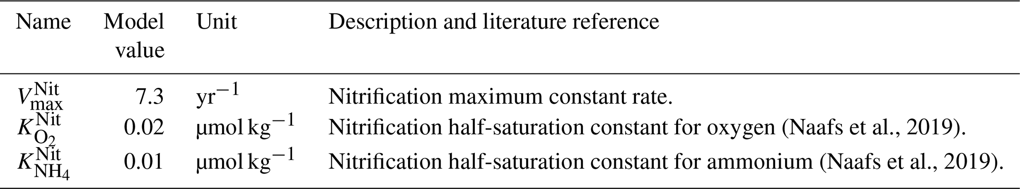
Nitrification is the process of oxidising ammonia to nitrate. The rate of nitrification (O_Nit) is determined by a two-substrate Michaelis–Menten formulation and allows for the limitation by both ammonium and oxygen (Naafs et al., 2019).

$$\begin{array}{}\text{(12)}& \begin{array}{rl}& {\mathrm{O}}_{\mathrm{Nit}}=V_{\max }^{\mathrm{Nit}}\\ & {\displaystyle \frac{{\mathrm{O}}_{\mathrm{2}}\times {\mathrm{NH}}_{\mathrm{4}}^{+}}{\left(K_{{\mathrm{O}}_{\mathrm{2}}}^{\mathrm{Nit}}\times K_{{\mathrm{NH}}_{\mathrm{4}}}^{\mathrm{Nit}}\right)+\left(K_{{\mathrm{O}}_{\mathrm{2}}}^{\mathrm{Nit}}\times {\mathrm{NH}}_{\mathrm{4}}^{+}\right)+\left(K_{{\mathrm{NH}}_{\mathrm{4}}}^{\mathrm{Nit}}\times {\mathrm{O}}_{\mathrm{2}}\right)+\left({\mathrm{O}}_{\mathrm{2}}\times {\mathrm{NH}}_{\mathrm{4}}^{+}\right)}}\\ & \min \left[{\mathrm{NH}}_{\mathrm{4}}^{+},{\displaystyle \frac{\mathrm{16}}{\mathrm{138}}}{\mathrm{O}}_{\mathrm{2}}\right]\end{array}\end{array}$$

where $V_{\max }^{\mathrm{Nit}}$ is the maximum rate of nitrification, $K_{{\mathrm{O}}_{\mathrm{2}}}^{\mathrm{Nit}}$ and $K_{{\mathrm{NH}}_{\mathrm{4}}}^{\mathrm{Nit}}$ are the half-saturation constants for oxygen and ammonium (Naafs et al., 2019), the values, units and brief description of equation constants are provided in Table 4.

Table 3 Nutrient cycle fluxes applied to NutGEnIE. These parameters relate to Eqs. (5), (10) and (13).

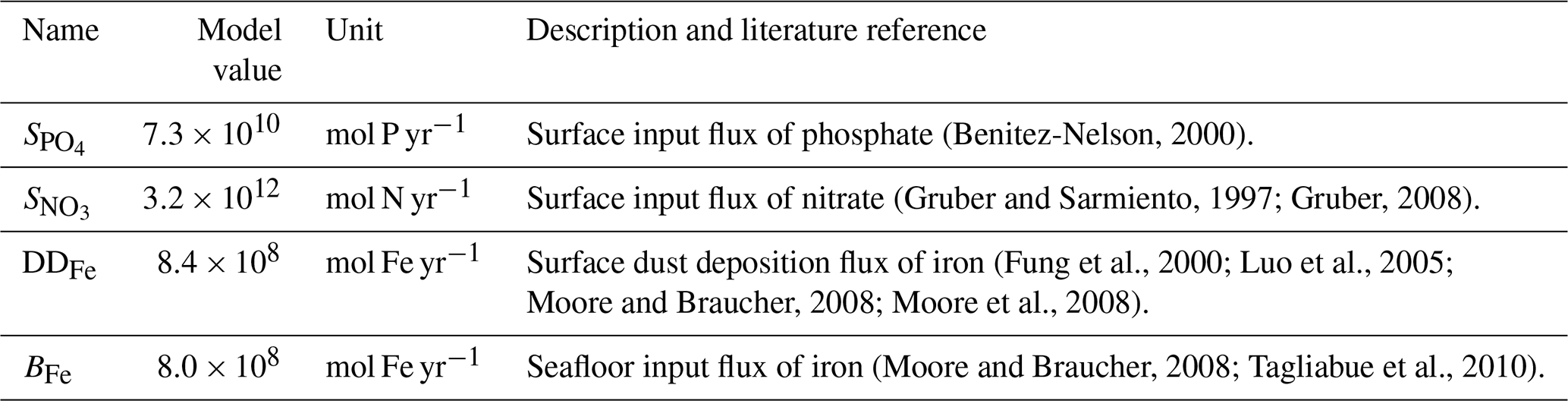
Table 4 Biogeochemical parameters of NutGEnIE relating to Nitrification. The parameters relate to Eq. (12).

The novel aspects of the nitrogen cycle in NutGEnIE are the inclusion of an input flux $S_{{\mathrm{NO}}_{\mathrm{3}}}$ and removal flux mechanism Eqs. (1) and (2); the input flux $S_{{\mathrm{NO}}_{\mathrm{3}}}$ can also be adjusted which will support the future work to investigate the ULN.

2.3.5 Iron cycle and uptake

NutGEnIE governing equations for Fe_T are below.

$$\begin{array}{}\text{(13)}& {\displaystyle }& {\displaystyle \frac{\partial {\mathrm{Fe}}_{\mathrm{T}}}{\partial t}}=-{\mathrm{\Gamma }}_{\mathrm{Fe}}^{\mathrm{OPhy}}-{\mathrm{\Gamma }}_{\mathrm{Fe}}^{\mathrm{Diaz}}+\mathit{\lambda }\mathrm{DOFe}+{\mathrm{DD}}_{\mathrm{Fe}}+B_{\mathrm{Fe}}-k_{\mathrm{sc}}{\mathrm{Fe}}^{\prime }\text{(14)}& {\displaystyle }& {\displaystyle \frac{\partial \mathrm{DOFe}}{\partial t}}=v\left({\mathrm{\Gamma }}_{\mathrm{Fe}}^{\mathrm{NOPhy}}+{\mathrm{\Gamma }}_{\mathrm{Fe}}^{\mathrm{NDiaz}}\right)-\mathit{\lambda }\mathrm{DOFe}\end{array}$$

The governing equation for iron contains an additional term, DD_Fe, that represents iron supplied via dust deposition. B_Fe represent an additional configurable input flux of iron applied to the seafloor layer. The prescribed dust deposition is achieved by a NutGEnIE forcing mechanism following a re-gridding from Mahowald et al. (2006), see Fig. S3. The processes associated with iron follow the methodology of Parekh et al. (2005). k_sc is a scavenging rate term that acts on free dissolved iron (Fe^′) throughout the water column. Honeyman et al. (1988) observed that particle concentration influences scavenging; its rate in NutGEnIE takes this into account by using a power law function to determine the scavenging rate:

$$\begin{array}{}\text{(15)}& k_{\mathrm{sc}}=\mathit{\tau }{k}_{\mathrm{0}}{\left(C_{\mathrm{p}}\right)}^{\mathit{\varphi }}\end{array}$$

where k₀ is the scavenging rate (when particles are abundant), C_p is the particle concentration, and ϕ is a constant coefficient. The rate of scavenging is calculated as part of particle remineralisation which in turn is calculated as a function of the rate of creation of new particles in the upper ocean, which in turn is calculated from the nutrient uptake rate.

As Honeyman et al. (1988) empirically determined k₀ and ϕ using thorium, the scavenging rate is scaled by τ (Parekh et al., 2005). The values, units and brief description of equation constants are provided in Table 1. The novel aspects of the iron cycle in NutGEnIE are the inclusion of an input flux B_Fe and removal flux mechanism (Eqs. 1 and 2); the input fluxes DD_Fe and B_Fe can also be adjusted as is necessary to support the future work to investigate the ULN. Addition of a seafloor flux alongside the existing surface flux DD_Fe is a more realistic representation of ocean iron cycle fluxes (Tagliabue et al., 2017). The processes associated with ligand complexation have also been extended as discussed in Sect. 2.3.6.

2.3.6 Ligand scheme enhancement in NutGEnIE

The iron cycle involves two processes that act on Fe^′, scavenging and complexation. Fe^′ an be scavenged and is lost as particulate iron, which thereafter is not available for biological uptake. Secondly, Fe^′ can be complexed with a free ligand (L^′) to form complexed iron (FeL). Complexed iron can in turn disassociate, reverting to free iron and a free ligand. An equilibrium is established so that Fe^′ + L^′ FeL. Both Fe^′ and FeL are available for biological uptake. Scavenging, complexation, and biological uptake processes are shown in Fig. 3. Total iron (Fe_T) is the sum of free and complexed iron Fe_T = Fe^′ + FeL. Total ligand (L_T) is the sum of free and complexed ligands L_T = L^′ + FeL. It is Fe_T and L_T that are maintained as tracers with L_T having a fixed inventory, Table S2.

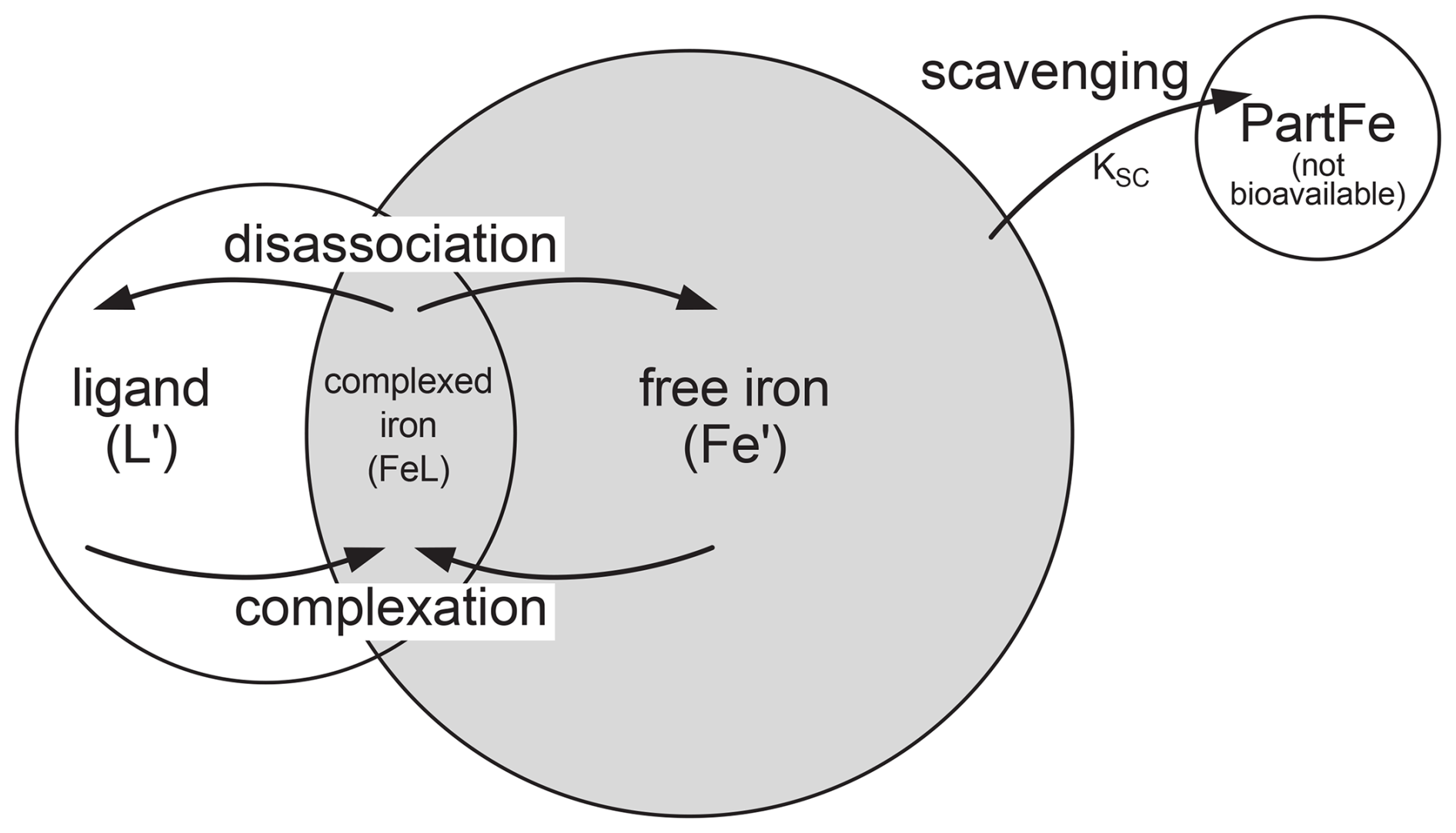
Figure 3 Schematic of iron scavenging, complexation, and biological availability. The rate of scavenging in represented by K_SC. Both Fe^′ and FeL are biologically available (shaded area). Complexation is the combination of Fe^′ and L^′ to form complexed iron (FeL). FeL can disassociate to Fe^′ and L^′.

Complexation of Fe^′ and L^′ to FeL occurs on the timescales of minutes to hours (Witter et al., 2000) such that it is valid to assume that the complexation reaction goes to equilibrium. An equilibrium relationship constant (k_FeL), where k_FeL = [FeL]/[Fe^′][L^′], can be used to determine the speciation of iron (Parekh et al., 2004). A ligand strength, or stability constant, (log (k_FeL)=11.0) is used which is based on field and laboratory studies and sensitivity analysis (Parekh et al., 2004). Higher values of the stability constant, log (k_FeL), imply a stronger binding ligand, and lower values a weaker binding ligand. The ligand scheme described above is based on the work of Archer and Johnson (2000) and Parekh et al. (2004, 2005).

However, research has indicated differing ligand classes with differing binding strengths as well as a varying distribution of ligands through the water column. Schemes with dual ligand classes have been proposed with a strong binging ligand L₁ in surface waters and a moderate binding class L₂ throughout the water column (Hunter and Boyd, 2007; Ye et al., 2009; Misumi et al., 2013; Völker and Tagliabue, 2015). Differing distributions of L₁ and L₂ are of interest when considering global modelling (Misumi et al., 2013; Völker and Tagliabue, 2015; Boyd and Tagliabue, 2015; Ye et al., 2020). The behaviour of ligand class L₂ is analogous with the single ligand class scheme described above (Parekh et al., 2005). The net effect of schemes with dual ligand classes is to have strong binging ligands at the surface. This stronger binging surface ligand behaviour has been addressed by creating a dynamic stability constant that can be configured for each NutGEnIE depth level. The binding characteristics of ligands are represented by a stability constant (k_FeL) which, in NutGEnIE, has been made configurable independently for each depth level. A default value of k_FeL is configured with the ability to override this at each depth level by providing a depth level specific stability constant $k_{\mathrm{FeL}}^n$, where n denotes the layer, from 16 (surface layer) to 1 (deepest layer). The existence of a strong binging ligand class predominantly present in the upper water column is represented by setting a higher value of $k_{\mathrm{FeL}}^{\mathrm{16}}$ ($\log \left(k_{\mathrm{FeL}}^{\mathrm{16}}\right)=\mathrm{11.4}$) in the surface layer of NutGEnIE. For all other layers the value is the default value.

2.3.7 Organic matter (OM) remineralisation

OM is split into two fractions, labile and refractory (refrac). OM is remineralised through the water column according to Eq. (16), an exponential function of depth (Reinhard et al., 2020).

$$\begin{array}{}\text{(16)}& \begin{array}{rl}{F}^{\mathrm{POM}}\left(z\right)& =F^{\mathrm{POM}}\left(z=z_{\mathrm{0}}\right)\left(r_{\mathrm{labile}}^{\mathrm{POM}}{e}^{\left[\frac{z_{\mathrm{0}}-z}{l_{\mathrm{labile}}}\right]}\right.\\ & \left.+\left(\mathrm{1}-r_{\mathrm{labile}}^{\mathrm{POM}}\right)e^{\left[\frac{z_{\mathrm{0}}-z}{l_{\mathrm{refrac}}}\right]}\right)\end{array}\end{array}$$

F^POM(z) is the POM flux at depth z. z₀ is the depth of the base of the photic zone. The labile fraction of POM is $r_{\mathrm{labile}}^{\mathrm{POM}}$, consequently, the refractory fraction of POM is ($\mathrm{1}-r_{\mathrm{labile}}^{\mathrm{POM}}$). l_labile and l_refrac are the e-folding depths of remineralisation for labile POM and refractory POM. The values, units and brief description of equation constants are provided in Table 7.

OM decomposition is partitioned via a series of redox reactions: initially aerobic respiration utilising O₂ as the electron acceptor, secondly denitrification utilising NO${}_{\mathrm{3}}^{-}$ as the electron acceptor, and lastly sulfate reduction utilising SO${}_{\mathrm{4}}^{\mathrm{2}-}$ as the electron acceptor. Electron acceptors (O₂, NO${}_{\mathrm{3}}^{-}$, and SO${}_{\mathrm{4}}^{\mathrm{2}-}$) are consumed according to decreasing free energy yields (Froelich et al., 1979). Consumption rates of electron acceptors in the process of OM remineralisation are relative to R_i in Eqs. (17)–(19) and take account of both electron acceptors abundance and the inhibitory effect of electron acceptors with higher free energy yield (Reinhard et al., 2020). Equation (20) can be considered to represent aerobic respiration, Eq. (21) represents nitrate reduction/denitrification, and Eq. (22) represents sulfate reduction.

$$\begin{array}{}\text{(17)}& {\displaystyle }& {\displaystyle }{R}_{{\mathrm{O}}_{\mathrm{2}}}={\displaystyle \frac{\left[{\mathrm{O}}_{\mathrm{2}}\right]}{K_{{\mathrm{O}}_{\mathrm{2}}}+\left[{\mathrm{O}}_{\mathrm{2}}\right]}}\text{(18)}& {\displaystyle }& {\displaystyle }{R}_{{\mathrm{NO}}_{\mathrm{3}}}={\displaystyle \frac{\left[{\mathrm{NO}}_{\mathrm{3}}^{-}\right]}{K_{{\mathrm{NO}}_{\mathrm{3}}}+\left[{\mathrm{NO}}_{\mathrm{3}}^{-}\right]}}{\displaystyle \frac{K_{{\mathrm{O}}_{\mathrm{2}}}^i}{K_{{\mathrm{O}}_{\mathrm{2}}}^i+\left[{\mathrm{O}}_{\mathrm{2}}\right]}}\text{(19)}& {\displaystyle }& {\displaystyle }{R}_{{\mathrm{SO}}_{\mathrm{4}}}={\displaystyle \frac{\left[{\mathrm{SO}}_{\mathrm{4}}^{\mathrm{2}-}\right]}{K_{{\mathrm{SO}}_{\mathrm{4}}}+\left[{\mathrm{SO}}_{\mathrm{4}}^{\mathrm{2}-}\right]}}{\displaystyle \frac{K_{{\mathrm{O}}_{\mathrm{2}}}^i}{K_{{\mathrm{O}}_{\mathrm{2}}}^i+\left[{\mathrm{O}}_{\mathrm{2}}\right]}}{\displaystyle \frac{K_{{\mathrm{NO}}_{\mathrm{3}}}^i}{K_{{\mathrm{NO}}_{\mathrm{3}}}^i+\left[{\mathrm{NO}}_{\mathrm{3}}^{-}\right]}}\end{array}$$

where R_i indicates the relative fraction of each electron acceptor consumed, K_i are the half-saturation constants for each redox reaction and $K_i^i$ are the inhibition constants to reduce redox reactions of lower free energy yields. The values, units and brief description of equation constants are provided in Table 6.

Table 5 Biogeochemical parameters of NutGEnIE relating to the iron cycle. The parameters relate to the text of Sect. 2.3.6.

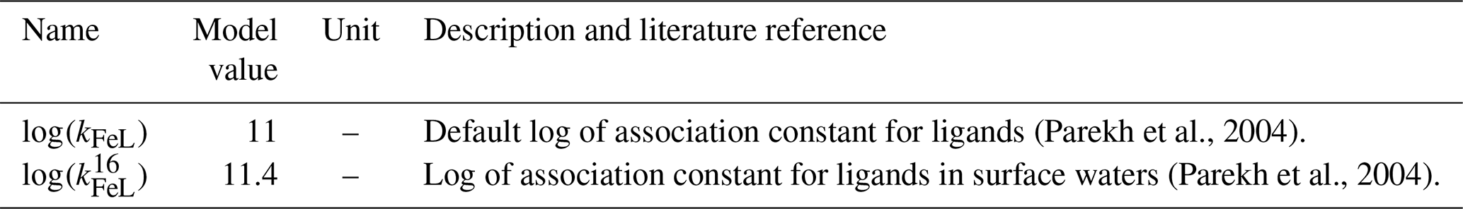
Table 6 Biogeochemical parameters of NutGEnIE relating to remineralisation. These parameters relate to Eqs. (16)–(22). Where the model value of the parameter differs from the literature reference value, the literature value is provided.

Redfield stoichiometry defines the primary elemental ratios of OM; in addition, OM contains Fe determined by the parameter $R_{\mathrm{Fe}}^{\mathrm{OPhy}}$, see Table 2, resulting in elemental ratios of C : N : P : Fe = 106 : 16 : 1 : $R_{\mathrm{Fe}}^{\mathrm{OPhy}}$. The remineralisation process follows the redox pathways of Eqs. (20)–(22) (Froelich et al., 1979).

$$\begin{array}{}\text{(20)}& {\displaystyle }\begin{array}{rl}\mathrm{OM}& +\mathrm{138}{\mathrm{O}}_{\mathrm{2}}⟶\mathrm{106}{\mathrm{CO}}_{\mathrm{2}}+\mathrm{16}{\mathrm{NH}}_{\mathrm{4}}+{\mathrm{H}}_{\mathrm{3}}{\mathrm{PO}}_{\mathrm{4}}\\ & +R_{\mathrm{Fe}}^{\mathrm{OPhy}}\mathrm{Fe}+\mathrm{122}{\mathrm{H}}_{\mathrm{2}}\mathrm{O}\end{array}\text{(21)}& {\displaystyle }\begin{array}{rl}\mathrm{OM}& +\mathrm{94.4}{\mathrm{HNO}}_{\mathrm{3}}⟶\mathrm{106}{\mathrm{CO}}_{\mathrm{2}}+\mathrm{55.2}{\mathrm{N}}_{\mathrm{2}}+{\mathrm{H}}_{\mathrm{3}}{\mathrm{PO}}_{\mathrm{4}}\\ & +R_{\mathrm{Fe}}^{\mathrm{OPhy}}\mathrm{Fe}+\mathrm{177.2}{\mathrm{H}}_{\mathrm{2}}\end{array}\text{(22)}& {\displaystyle }\begin{array}{rl}\mathrm{OM}& +\mathrm{53}{\mathrm{SO}}_{\mathrm{4}}^{\mathrm{2}-}⟶\mathrm{106}{\mathrm{CO}}_{\mathrm{2}}+\mathrm{16}{\mathrm{NH}}_{\mathrm{4}}+\mathrm{53}{S}^{\mathrm{2}-}\\ & +{\mathrm{H}}_{\mathrm{3}}{\mathrm{PO}}_{\mathrm{4}}+R_{\mathrm{Fe}}^{\mathrm{OPhy}}\mathrm{Fe}+\mathrm{106}{\mathrm{H}}_{\mathrm{2}}\mathrm{O}\end{array}\end{array}$$

OM decomposition when oxygen levels are low leads to the use of nitrate as an alternative electron acceptor. Therefore, Eq. (21) above represents denitrification in NutGEnIE.

2.3.8 NutGEnIE configuration parameters

The NutGEnIE model has an implicit ecosystem and therefore appropriate values for constants are not immediately apparent. The constants associated with the processes set out in sections above are based on previous calibrations of cGEnIE (Ridgwell et al., 2007; Monteiro et al., 2012; Reinhard et al., 2020; van de Velde et al., 2021) with adjustments associated with the open nutrient cycle configuration. The parameters associated with nutrient tracers, nutrient uptake, remineralisation, nitrification, and iron cycle are outlined in Tables 1–6. The atmosphere of NutGEnIE is set to and maintained at a pre-industrial CO₂ concentration of 278 ppm (part per million).

In many cases parameters, particularly those associated with nutrient uptake, have been determined as the result of a calibration or tuning exercise. Parameters were adjusted to result in a combination that showed best agreement with observed nutrient distributions, the scale of pertinent processes (e.g., export and nitrogen fixation), and the spatial variations of nutrient uptake limitations. The determination of the best parameter combination used the techniques outlined in Sect. 3 information relating to the tuning exercise is provided in Sect. S1.3 in the Supplement.

3 Model validation results

The cGEnIE model has been used extensively, with many studies examining the validity of the cGEnIE approach and experiment results (Ridgwell et al., 2007; Monteiro et al., 2012; Tagliabue et al., 2016; Reinhard et al., 2020; van de Velde et al., 2021). A complete validation analysis of cGEnIE and its capabilities of representing the ocean and its processes is not undertaken here. The aim in the validation in this paper is to asses the pertinent biogeochemical distributions and processes that are relevant to the proposed use of NutGEnIE. NutGEnIE will be used to consider the effect nutrient supply has on PP and this informs the biogeochemical processes considered in the validation process. Nutrient concentrations and distributions are evaluated because they influence PP which is central to the intended purpose (identification of the ULN). The processes of photosynthesis, respiration and remineralisation occur at differing depths of the ocean water column and each exert an influence on the concentration of dissolved oxygen. The concentration of dissolved oxygen is therefore a useful indicator of biogeochemical processes and, hence, also worthy of evaluation here. In Sect. 2.2 above, the concept that NutGEnIE represents PP by nutrient uptake and the subsequent formation or organic matter was discussed. In NutGEnIE a proportion of this organic matter sinks from the ocean surface and therefore POC export is also compared to observations.

3.1 Datasets and methods

The World Ocean Atlas (WOA) 2018 provides annual climatology data based on observed ocean properties that are utilised for comparison purposes. These properties include temperature (Locarnini et al., 2018), salinity (Zweng et al., 2018), phosphate concentrations (Garcia et al., 2018a), nitrate concentrations (Garcia et al., 2018a) and dissolved oxygen concentrations (Garcia et al., 2018b). The WOA datasets are provided with a spatial resolution of 1°×1° grid and 102 depth levels from surface to 5500 m.

The GEOTRACES Intermediate Data Product 2021 dataset contains data from cruises measuring multiple hydrographic parameters, trace metals, and isotopes (GEOTRACES Intermediate Data Product Group, 2021; GEOTRACES, 2022). GEOTRACES provides depth profiles of ocean dissolved iron concentration measurements in the Atlantic, Pacific and Southern Oceans that were compared to NutGEnIE concentrations using depth profiles. Cruises GA02 (March–April 2011) and GIPY05 (February–April 2008) covered the Atlantic Ocean and Southern Ocean respectively while GPc06 (August–September 2005) and GP19 (December 2014–February 2015) provided coverage of the Pacific Ocean.

The Oregon State University Ocean Productivity group (Ocean Productivity, 2024) provide computations, based on observational data, of vertically integrated net PP (NPP). Differing methodologies for the computation of NPP are supported by the Ocean Productivity group. The observational rate of NPP (g C m⁻² d⁻¹) used for comparison purposes here is the mean of values from the VGPM (Behrenfeld and Falkowski, 1997), Eppley-VGPM (Carr et al., 2006) and CbPM (Westberry et al., 2008) methodologies. The observation-based estimates are provided with a spatial resolution of $\mathrm{1}/\mathrm{6}\mathit{°}\times \mathrm{1}/\mathrm{6}\mathit{°}$ grid, that is, a 2160×1080 grid.

3.1.1 Rates and distribution of nitrogen fixation and denitrification

It is important that the model has a realistic level of nitrogen fixation as the dynamic between diazotrophs and other phytoplankton will influence how the model reacts to nutrient perturbations. Estimates of ocean N₂ fixation have tended to increase over the previous three decades with some key global marine values being (all values provided in Tg N yr⁻¹) 125±41 (Gruber and Sarmiento, 1997); 132 (Codispoti et al., 2001); 121 (Galloway et al., 2004); 135±51 (Gruber, 2004); 140±9 (Luo et al., 2012); and 163±49 (Wang et al., 2019).

Alongside work to constrain the scale of global marine N₂ fixation, work has progressed to determine the spatial distribution of diazotrophs. Spatial restrictions on the prevalence of marine nitrogen fixation have been summarised in Fig. 2 of Sohm et al. (2011), Fig. 3a of Wang et al. (2019), and Fig. 4 of Zehr and Capone (2020). In each of these figures marine nitrogen fixation is mostly limited to within 30° either side of the equator. Sohm et al. (2011) and Wang et al. (2019) both indicate that in the Pacific and Atlantic basins nitrogen fixation rates are elevated in the northern hemisphere compared to the southern hemisphere. Wang et al. (2019) and Zehr and Capone (2020) highlight that whilst marine nitrogen fixation is mostly limited to a band from 30° N to 30° S it is somewhat reduced at the equator, and this is particularly so in the Pacific Ocean. The area of reduced nitrogen fixation in the equatorial Pacific Ocean corresponds to an area of nutrient supply from deep water upwelling.

Estimates of denitrification are routinely greater than those for N₂ fixation in marine nitrogen budgets. Example of annual global marine denitrification are 175±28 (Gruber and Sarmiento, 1997); 450 (Codispoti et al., 2001); 322 (Galloway et al., 2004); 245±54 (Gruber, 2004); and 200±52 (Wang et al., 2019) (all values provided in Tg N yr⁻¹). Wang et al. (2019) provide location of fixed nitrogen loss due to (a) water column denitrification and anammox and (b) sedimentary denitrification and anammox. Areas of significant water column denitrification include the northern Indian Ocean, northern Pacific Ocean, eastern equatorial Pacific Ocean and the eastern equatorial Atlantic Ocean (Wang et al., 2019). Sedimentary denitrification is more evenly distributed across the ocean basins with intensification closer to coastal locations (Wang et al., 2019).

3.1.2 Comparison techniques

WOA and Ocean Productivity datasets are re-gridded both horizontally and vertically to match NutGEnIE prior to comparison. Hereafter comparisons which utilise the re-gridded datasets are referred to as WOAR and OPR for WOA and Ocean Productivity respectively.

Thermohaline transects are used to represent and compare properties of the ocean interior following a similar approach to that detailed by Yool et al. (2021). The aim of the transects is to generally follow water masses from recently ventilated young deep water in the North Atlantic, through the Southern Ocean, to older deep waters in the North Pacific, and basin zonal means are used throughout the transect. For reference, NutGEnIE age of water (i.e., years since ventilation) details are provided in Fig. S4.

3.1.3 Statistical evaluation

The alignment processes detailed in the previous two sections also facilitated statistical analysis of properties common to NutGEnIE and WOAR, that is temperature, salinity, [PO${}_{\mathrm{4}}^{\mathrm{3}-}$], [NO${}_{\mathrm{3}}^{-}$] and [O₂]. The statistical analysis was conducted for the surface ocean as well as for the thermohaline transects. The statistical calculation only considers cells that are present in both the NutGEnIE and WOAR datasets and computes the mean and standard deviation for each dataset. Correlation analysis between the two datasets can then provide a Pearson correlation coefficient (r) and a p-value resulting from a test of the null hypothesis that there is no relationship between the datasets.

Normalising each dataset by calculating the ratio of each model standard deviation to the observed standard deviation, when combined with correlation coefficients, allows a graphical representation of the skill of NutGEnIE using a Taylor diagram (Taylor, 2001). The normalised NutGEnIE standard deviation will vary either side of 1, with a value of 1 indicating the same standard deviation in the model results as in the observed data. The correlation is indicated by the r value, angular distance θ from the origin is controlled by the normalised standard deviation and the correlation coefficient, with a correlation of 1 on the x-axis. The normalised centred root-mean-square (RMS) difference between NutGEnIE results and observed data is proportional to the distance from points on the plot of perfect agreement.

3.1.4 Spatial variation of limiting factors and nutrients

Given the proposed use of the model to investigate the nature of nutrient limitation, additional diagnostic outputs have been added. The diagnostics are based on the nutrient uptake equations for other phytoplankton and diazotrophs (Eqs. 3 and 4 respectively). The temperature component γ^T can have values greater than one, therefore the temperature limiting factor (LF_Temp) is determined as the minimum of γ^T and 1. This ensures that LF_Temp only detects scenarios where temperature acts to constrain nutrient uptake. It is then possible to represent each of these limiting factors on a single figure by setting them each to represent a channel of RGB colour. Nutrient limitation is represented by green; temperature limitation is represented by red; and light limitation is represented by blue. Limitation by multiple factors is represented by the resulting mixed colour as displayed on the Maxwell triangle. The limiting factor values are calculated as follows at each time step of the model processing.

$$\begin{array}{}\text{(23)}& {\displaystyle }& {\displaystyle }{\mathrm{LF}}_{\mathrm{Temp}}=\min \left[{\mathit{\gamma }}^T,\mathrm{1}\right]\text{(24)}& {\displaystyle }& {\displaystyle }{\mathrm{LF}}_{\mathrm{Light}}={\mathit{\gamma }}^I\text{(25)}& {\displaystyle }& {\displaystyle }{\mathrm{LF}}_{\mathrm{Nut}}^{\mathrm{OPhy}}=\min \left[{\displaystyle \frac{{\mathrm{PO}}_{\mathrm{4}}^{\mathrm{3}-}}{{\mathrm{PO}}_{\mathrm{4}}^{\mathrm{3}-}+K_{\mathrm{P}}}}{\displaystyle \frac{\mathrm{DIN}}{\mathrm{DIN}+K_{\mathrm{N}}}};{\displaystyle \frac{\mathrm{Fe}}{\mathrm{Fe}+K_{\mathrm{Fe}}}}\right]\end{array}$$

$$\begin{array}{}\text{(26)}& {\mathrm{LF}}_{\mathrm{Nut}}^{\mathrm{Diaz}}=\min \left[{\displaystyle \frac{{\mathrm{PO}}_{\mathrm{4}}^{\mathrm{3}-}}{{\mathrm{PO}}_{\mathrm{4}}^{\mathrm{3}-}+{\mathrm{K}}_{\mathrm{P}}}};{\displaystyle \frac{\mathrm{Fe}}{\mathrm{Fe}+K_{\mathrm{Fe}}^{\mathrm{Diaz}}}}\right]\end{array}$$

In a similar manner, the limiting nutrient at each time step of model processing is determined by considering each Michaelis-Menten term; this facilitates determination of the PLN at each time step. For each cell and time step the nutrient identified as the PLN is assigned 1, the other nutrients are assigned 0. This facilitates the determination of a limiting nutrient term (e.g., LN${}_{\mathrm{P}}^{\mathrm{OPhy}}$) as outlined in Eqs. (27)–(31).

$$\begin{array}{}\text{(27)}& {\displaystyle }\begin{array}{rl}\mathrm{if}& {\displaystyle \frac{{\mathrm{PO}}_{\mathrm{4}}^{\mathrm{3}-}}{{\mathrm{PO}}_{\mathrm{4}}^{\mathrm{3}-}+K_{\mathrm{P}}}}<{\displaystyle \frac{\mathrm{DIN}}{\mathrm{DIN}+K_{\mathrm{N}}}}\mathrm{and}{\displaystyle \frac{{\mathrm{PO}}_{\mathrm{4}}^{\mathrm{3}-}}{{\mathrm{PO}}_{\mathrm{4}}^{\mathrm{3}-}+K_{\mathrm{P}}}}\\ & <{\displaystyle \frac{\mathrm{Fe}}{\mathrm{Fe}+K_{\mathrm{Fe}}}}\mathrm{then}{\mathrm{LN}}_{\mathrm{P}}^{\mathrm{OPhy}}=\mathrm{1}\mathrm{else}{\mathrm{LN}}_{\mathrm{P}}^{\mathrm{OPhy}}=\mathrm{0}\end{array}\text{(28)}& {\displaystyle }\begin{array}{rl}\mathrm{if}& {\displaystyle \frac{\mathrm{DIN}}{\mathrm{DIN}+K_{\mathrm{N}}}}<{\displaystyle \frac{{\mathrm{PO}}_{\mathrm{4}}^{\mathrm{3}-}}{{\mathrm{PO}}_{\mathrm{4}}^{\mathrm{3}-}+K_{\mathrm{P}}}}\mathrm{and}{\displaystyle \frac{\mathrm{DIN}}{\mathrm{DIN}+K_{\mathrm{N}}}}\\ & <{\displaystyle \frac{\mathrm{Fe}}{\mathrm{Fe}+K_{\mathrm{Fe}}}}\mathrm{then}{\mathrm{LN}}_{\mathrm{N}}^{\mathrm{OPhy}}=\mathrm{1}\mathrm{else}{\mathrm{LN}}_{\mathrm{N}}^{\mathrm{OPhy}}=\mathrm{0}\end{array}\text{(29)}& {\displaystyle }\begin{array}{rl}\mathrm{if}& {\displaystyle \frac{\mathrm{Fe}}{\mathrm{Fe}+K_{\mathrm{Fe}}}}<{\displaystyle \frac{{\mathrm{PO}}_{\mathrm{4}}^{\mathrm{3}-}}{{\mathrm{PO}}_{\mathrm{4}}^{\mathrm{3}-}+K_{\mathrm{P}}}}\mathrm{and}{\displaystyle \frac{\mathrm{Fe}}{\mathrm{Fe}+K_{\mathrm{Fe}}}}\\ & <{\displaystyle \frac{\mathrm{DIN}}{\mathrm{DIN}+K_{\mathrm{N}}}}\mathrm{then}{\mathrm{LN}}_{\mathrm{Fe}}^{\mathrm{OPhy}}=\mathrm{1}\mathrm{else}{\mathrm{LN}}_{\mathrm{Fe}}^{\mathrm{OPhy}}=\mathrm{0}\end{array}\text{(30)}& {\displaystyle }\begin{array}{rl}\mathrm{if}& {\displaystyle \frac{{\mathrm{PO}}_{\mathrm{4}}^{\mathrm{3}-}}{{\mathrm{PO}}_{\mathrm{4}}^{\mathrm{3}-}+K_{\mathrm{P}}}}<{\displaystyle \frac{\mathrm{Fe}}{\mathrm{Fe}+K_{\mathrm{Fe}}^{\mathrm{Diaz}}}}\mathrm{then}{\mathrm{LN}}_{\mathrm{P}}^{\mathrm{Diaz}}\\ & =\mathrm{1}\mathrm{else}{\mathrm{LN}}_{\mathrm{P}}^{\mathrm{Diaz}}=\mathrm{0}\end{array}\text{(31)}& {\displaystyle }\begin{array}{rl}\mathrm{if}& {\displaystyle \frac{\mathrm{Fe}}{\mathrm{Fe}+K_{\mathrm{Fe}}^{\mathrm{Diaz}}}}<{\displaystyle \frac{{\mathrm{PO}}_{\mathrm{4}}^{\mathrm{3}-}}{{\mathrm{PO}}_{\mathrm{4}}^{\mathrm{3}-}+K_{\mathrm{P}}}}\mathrm{then}{\mathrm{LN}}_{\mathrm{Fe}}^{\mathrm{Diaz}}\\ & =\mathrm{1}\mathrm{else}{\mathrm{LN}}_{\mathrm{Fe}}^{\mathrm{Diaz}}=\mathrm{0}\end{array}\end{array}$$

For each nutrient, annual mean values are then calculated for each cell. The PLN is then represented on a figure that utilises a RGB colour mechanism in which Fe PLN is represented by green, PO${}_{\mathrm{4}}^{\mathrm{3}-}$ PLN is represented by red, and DIN PLN is represented by blue.

3.1.5 Model initialisation and steady state

The NutGEnIE spin up experiment was executed for 50 kyr, sufficient for the N, P and Fe cycles to reach equilibrium and in excess of the residence time of each nutrient. The concentrations of global mean nutrients and dissolved oxygen throughout that spin up are provided in Fig. S5. The end state concentrations of nutrients and dissolved oxygen are as follows: global mean [PO${}_{\mathrm{4}}^{\mathrm{3}-}$] = 2.14 µmol kg⁻¹ (micromoles per kilogram); global mean [NO${}_{\mathrm{3}}^{-}$] = 28.5 µmol kg⁻¹; global mean [TDFe] = 0.73 nmol kg⁻¹ (nanomoles per kilogram); and global mean [O₂] = 176 µmol kg⁻¹. The NutGEnIE budget for each nutrient at steady state at the end of the 50 kyr spin up experiment is shown below in Fig. 4.

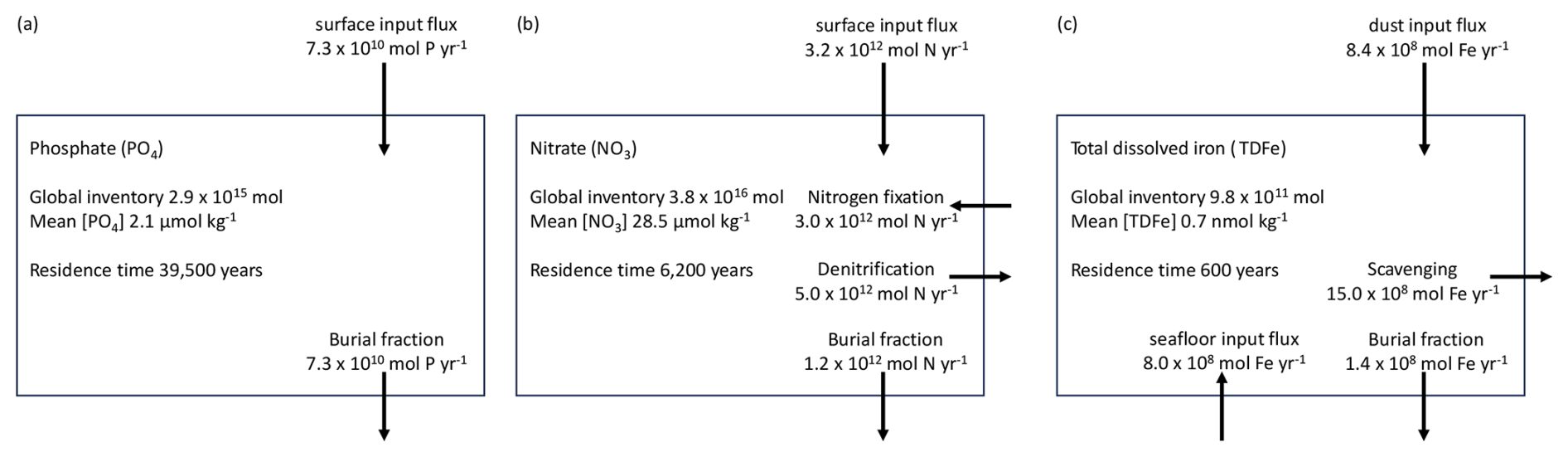
Figure 4 NutGEnIE nutrient budgets at end of 50 kyr spin up. (a) Phosphate budget. (b) Nitrate budget. (c) Total dissolved iron budget. Fluxes into and out of the ocean as a whole are shown, internal ocean cycling through nutrient uptake, remineralisation and nitrification are not shown.

3.2 Physical evaluation

Figure 5 shows the observations from the WOAR dataset, NutGEnIE results and deltas (differences between the two) for annual mean global sea surface temperature and thermohaline transects. It is noted that WOAR temperatures are in situ temperature, whereas potential temperature is used in NutGEnIE; however, the differences will be minimal and do not require an alignment conversion. NutGEnIE results are compared to WOAR salinity data in Fig. 6. NutGEnIE represents temperature and salinity reasonably well, but ocean physics is not the focus here, so the properties are not described in detail. Mean surface and interior (thermohaline transect) temperature and salinity values for both NutGEnIE and WOAR are provided in Table 7. NutGEnIE does exhibit some temperature biases; positive surfaces biases are present in the north and south Pacific with a negative surface bias in the Pacific subtropics (Fig. 5c). Similarly, biases exist in the temperature transect (Fig. 5f); for example, NutGEnIE has a general positive bias in the deep Atlantic and Southern Ocean. In the deep Pacific, NutGEnIE has a negative bias. Salinity biases of NutGEnIE are generally of low magnitude, within 1 psu. Surface biases (Fig. 6c) can be summarised as positive at higher latitudes and negative at mid latitudes. NutGEnIE salinity at depth greater than 1000 m have a positive bias with generally negative biases in the upper 500 m (Fig. 6f).

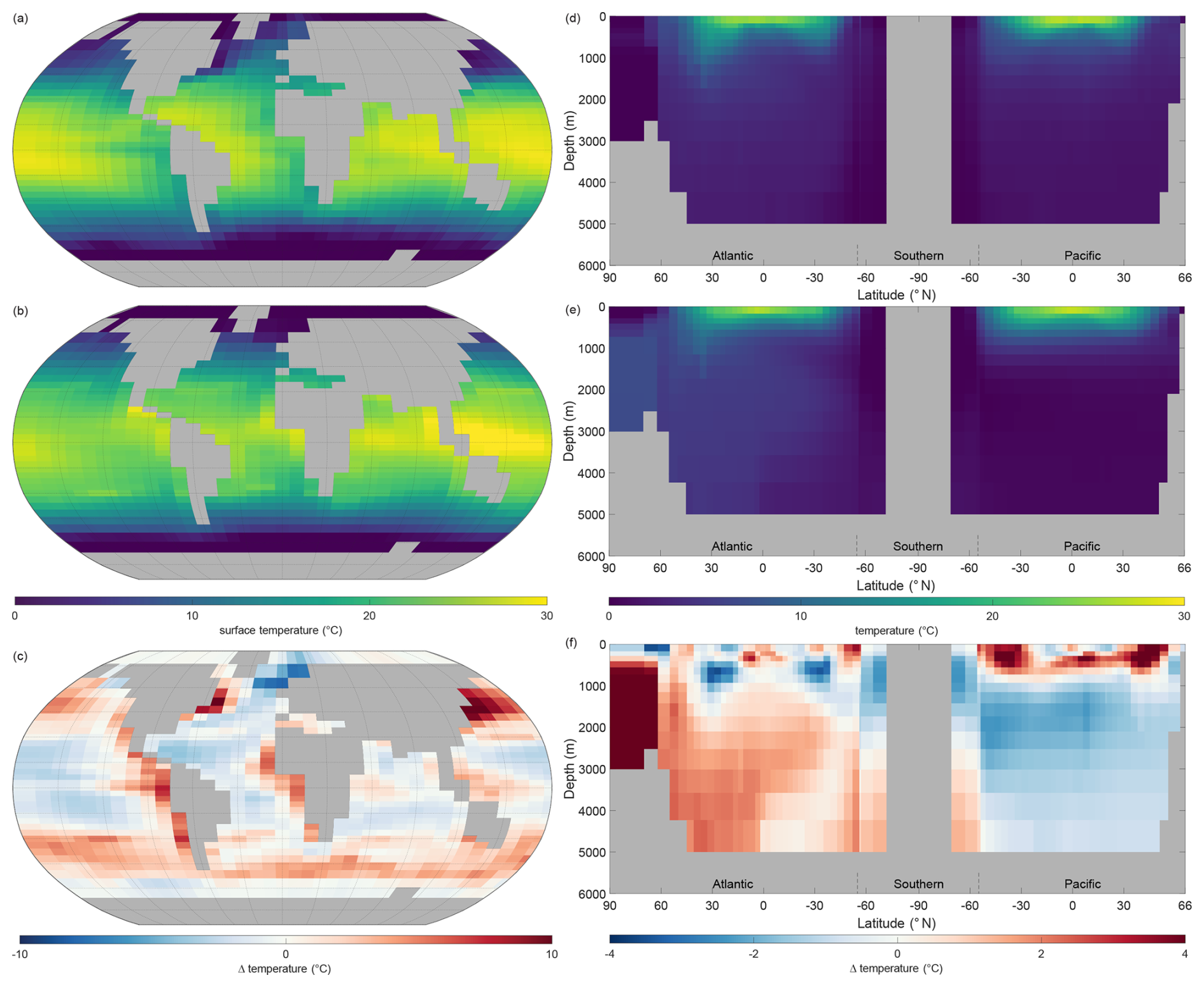
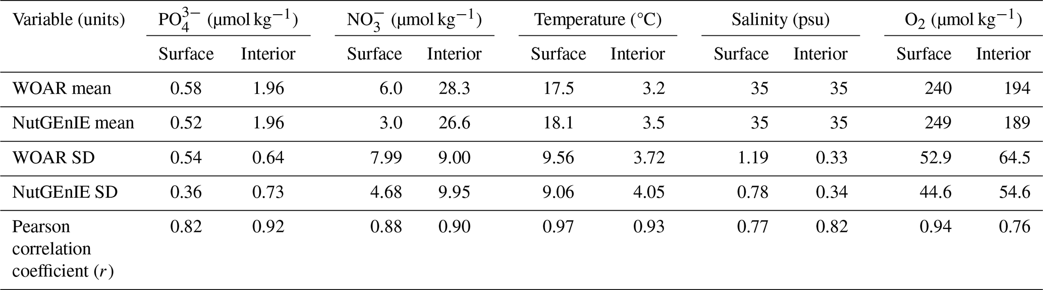
Figure 5 Annual mean global temperature. (a) Observed World Ocean Atlas Re-gridded (WOAR) sea surface temperature (SST). (b) NutGEnIE SST. (c) Delta SST (NutGEnIE – WOAR). (a–c) Based on surface level 0–80.8 m depth level. (d) Observed (WOAR) thermohaline transect zonal mean temperature. (e) NutGEnIE thermohaline transect zonal mean temperature. (f) Thermohaline transect temperature delta (NutGEnIE – WOAR). Temperature (and difference) in °C.

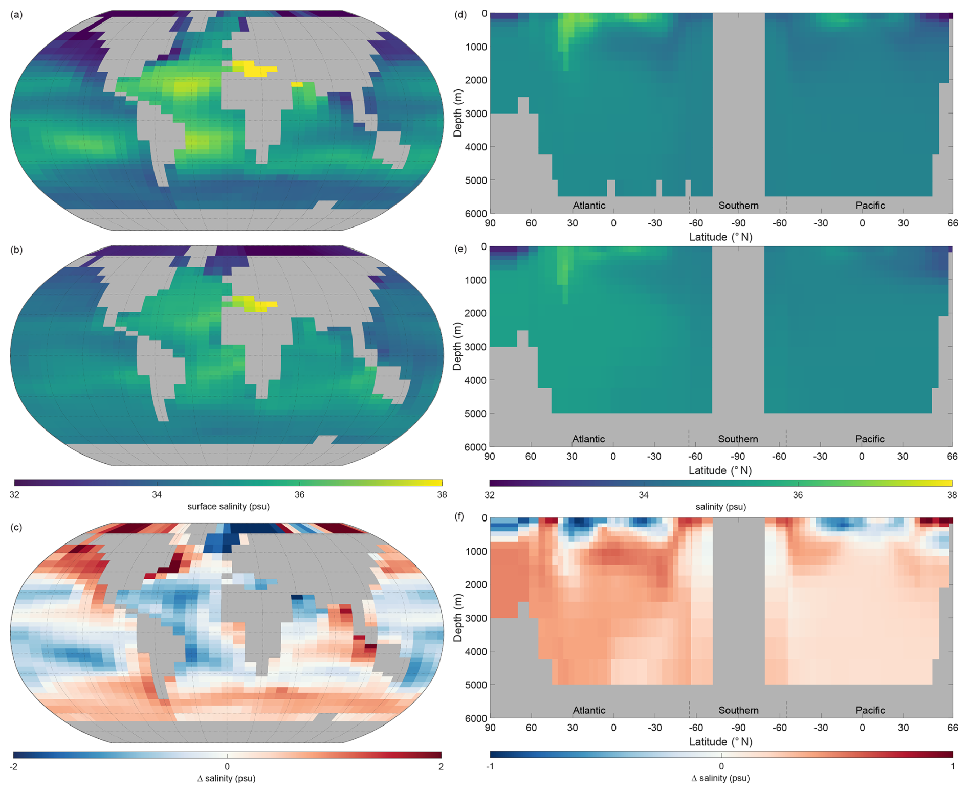
Figure 6 Annual mean global salinity. (a) Observed World Ocean Atlas Re-gridded (WOAR) sea surface salinity (SSS). (b) NutGEnIE SSS. (c) Delta SSS (NutGEnIE – WOAR). (a–c) Based on surface level 0–80.8 m depth level. (d) Observed (WOAR) thermohaline transect zonal mean salinity. (e) NutGEnIE thermohaline transect zonal mean salinity. (f) Thermohaline transect salinity delta (NutGEnIE – WOAR). Salinity (and difference) in psu.

Table 7 Statistical comparison of NutGEnIE to WOAR. Surface values relate to level depth of 0–80.8 m. Interior values reflect the thermohaline transects as defined in Sect. 3.1.2. SD = standard deviation. All correlations have a p-value of 0.

3.3 Biogeochemistry tracer evaluation (nutrients, oxygen)

3.3.1 Phosphate

The representation of phosphate and the other nutrients by NutGEnIE is particularly important if the model is to be suitable for experiments that examine the impacts of variations in nutrient supply. We have seen that the end state global mean concentration of phosphate is 2.14 µmol kg⁻¹; we now consider the spatial variation and compare to observational data.

The surface phosphate concentrations of NutGEnIE are largely a good representation of the observed concentration from WOAR. In general, NutGEnIE surface [PO${}_{\mathrm{4}}^{\mathrm{3}-}$] is slightly greater than observed [PO${}_{\mathrm{4}}^{\mathrm{3}-}$] at low latitudes and slightly less than observed [PO${}_{\mathrm{4}}^{\mathrm{3}-}$] at higher latitudes (Fig. 7a–c). The magnitude of differences in surface [PO${}_{\mathrm{4}}^{\mathrm{3}-}$] between NutGEnIE and observations are almost universally less than 0.5 µmol kg⁻¹. There are some specific differences to be noted; NutGEnIE surface [PO${}_{\mathrm{4}}^{\mathrm{3}-}$] is lower than observed in the North Pacific; between 45 and 60° S NutGEnIE surface [PO${}_{\mathrm{4}}^{\mathrm{3}-}$] is lower than observed; and NutGEnIE does not fully represent the supply of nutrients in upwelling areas of the equatorial Pacific and Benguela. The mean NutGEnIE annual mean global surface [PO${}_{\mathrm{4}}^{\mathrm{3}-}$] is 0.52 µmol kg⁻¹ with a standard deviation of 0.36 which compare to WOAR mean and standard deviations of 0.58 and 0.54 µmol kg⁻¹ respectively.

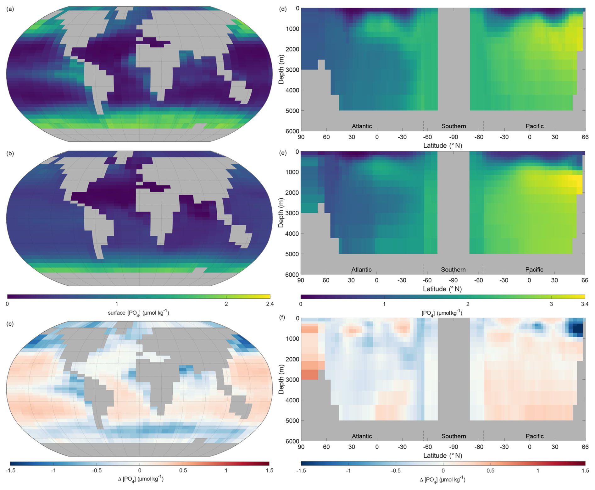
Figure 7 Annual mean global phosphate concentration ([PO${}_{\mathrm{4}}^{\mathrm{3}-}$]). (a) Observed World Ocean Atlas Re-gridded (WOAR) surface [PO${}_{\mathrm{4}}^{\mathrm{3}-}$]. (b) NutGEnIE surface [PO${}_{\mathrm{4}}^{\mathrm{3}-}$]. (c) Delta surface [PO${}_{\mathrm{4}}^{\mathrm{3}-}$] (NutGEnIE – WOAR). (a–c) Based on surface level 0–80.8 m depth level. (d) Observed (WOAR) thermohaline transect zonal mean [PO${}_{\mathrm{4}}^{\mathrm{3}-}$]. (e) NutGEnIE thermohaline transect zonal mean [PO${}_{\mathrm{4}}^{\mathrm{3}-}$]. (f) Thermohaline transect [PO${}_{\mathrm{4}}^{-}$] delta (NutGEnIE – WOAR). [PO${}_{\mathrm{4}}^{\mathrm{3}-}$] (and difference) in µmol kg⁻¹.

Ocean interior representation of phosphate by NutGEnIE is also successfully aligned to observed concentrations (Fig. 7d–f). The ocean interior Atlantic sector has somewhat lower [PO${}_{\mathrm{4}}^{\mathrm{3}-}$] than the Southern Ocean and [PO${}_{\mathrm{4}}^{\mathrm{3}-}$] is further elevated in the Pacific Ocean, reflecting the age of water masses, and increasing remineralisation (Fig. 7e). NutGEnIE also represents well the differing water masses in the Atlantic Ocean with the tongue of northward flowing Antarctic Intermediate Water rich in nutrients. Differences between NutGEnIE and observations are minimal apart from the northern Pacific Ocean at depths less than 1000 m where NutGEnIE [PO${}_{\mathrm{4}}^{\mathrm{3}-}$] are approximately 1.2 µmol kg⁻¹ less than observed concentrations. In general, NutGEnIE has a slight negative bias in [PO${}_{\mathrm{4}}^{\mathrm{3}-}$] in the Atlantic Ocean and a slight positive bias in [PO${}_{\mathrm{4}}^{\mathrm{3}-}$] in the Pacific Ocean. NutGEnIE represents the [PO${}_{\mathrm{4}}^{\mathrm{3}-}$] in the Southern Ocean in alignment with observations and there are consequently minimal differences in that sector of the thermohaline transect. The mean NutGEnIE annual mean [PO${}_{\mathrm{4}}^{\mathrm{3}-}$] of the thermohaline transect is 2.0 µmol kg⁻¹ with a standard deviation of 0.73 µmol kg⁻¹ which compare to WOAR mean and standard deviations of 2.0 and 0.64 µmol kg⁻¹ respectively.

3.3.2 Nitrate

Surface nitrate concentrations of NutGEnIE largely follow the spatial patterns of the observed concentration (Fig. 8a–c). In general, NutGEnIE surface [NO${}_{\mathrm{3}}^{-}$] are lower than the observed [NO${}_{\mathrm{3}}^{-}$], although this is less evident at low latitudes. The magnitude of differences in surface [NO${}_{\mathrm{3}}^{-}$] between NutGEnIE and observations are almost universally less than 10 µmol kg⁻¹. There are some specific differences to be noted which are similar to those identified for phosphate; NutGEnIE surface [NO${}_{\mathrm{3}}^{-}$] are lower than observed in the North Pacific; between 45 and 60° S NutGEnIE surface [NO${}_{\mathrm{3}}^{-}$] are ≈10 µmol kg⁻¹ lower than observed; and NutGEnIE does not fully represent the supply of nutrients in upwelling areas of the equatorial Pacific and Benguela. The mean NutGEnIE annual mean global surface [NO${}_{\mathrm{3}}^{-}$] is 3.0 µmol kg⁻¹ with a standard deviation of 4.68 µmol kg⁻¹ which compare to WOAR mean and standard deviations of 6.0 and 7.99 µmol kg⁻¹ respectively.

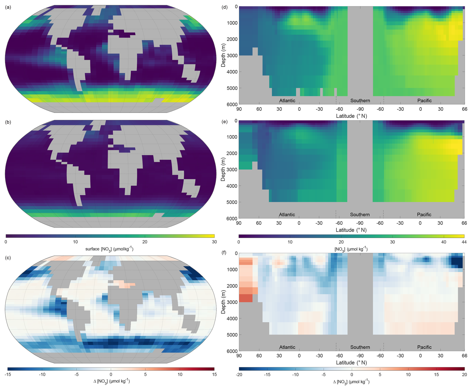
Figure 8 Annual mean global nitrate concentration ([NO${}_{\mathrm{3}}^{-}$]). (a) Observed World Ocean Atlas Re-gridded (WOAR) surface [NO${}_{\mathrm{3}}^{-}$]. (b) NutGEnIE surface [NO${}_{\mathrm{3}}^{-}$]. (c) Delta surface [NO${}_{\mathrm{3}}^{-}$] (NutGEnIE – WOAR). (a–c) Based on surface level 0–80.8 m depth level. (d) Observed (WOAR) thermohaline transect zonal mean [NO${}_{\mathrm{3}}^{-}$]. (e) NutGEnIE thermohaline transect zonal mean [NO${}_{\mathrm{3}}^{-}$]. (f) Thermohaline transect [NO${}_{\mathrm{3}}^{-}$] delta (NutGEnIE – WOAR). [NO${}_{\mathrm{3}}^{-}$] (and difference) in µmol kg⁻¹.

Ocean interior representation of nitrate by NutGEnIE are aligned to observation concentrations (Fig. 8d–f). The Atlantic sector has somewhat lower [NO${}_{\mathrm{3}}^{-}$] than the Southern Ocean and [NO${}_{\mathrm{3}}^{-}$] are further elevated in the Pacific Ocean, this again reflects the age of water masses, and increasing remineralisation. NutGEnIE also successfully represents differing water masses in the Atlantic Ocean with the tongue of northward flowing Antarctic Intermediate Water rich in nutrients. Differences between NutGEnIE and observations are less than 5 µmol kg⁻¹ apart from the northern Pacific Ocean at depths less than 1000 m where NutGEnIE [NO${}_{\mathrm{3}}^{-}$] are as much as 18 µmol kg⁻¹ less that observed concentrations. In general, NutGEnIE has a positive bias in [NO${}_{\mathrm{3}}^{-}$] in the Arctic, a negative bias in the Atlantic Ocean, a minimal negative bias in the Southern Ocean, and a positive bias in [NO${}_{\mathrm{3}}^{-}$] in the Pacific Ocean below 1000 m. The mean NutGEnIE annual mean [NO${}_{\mathrm{3}}^{-}$] of the thermohaline transect is 26.5 µmol kg⁻¹ with a standard deviation of 9.95 µmol kg⁻¹ which compare to WOAR mean and standard deviations of 28.3 and 9.0 µmol kg⁻¹ respectively.

3.3.3 Iron

In general, NutGEnIE broadly represents the observed iron depth profiles from the four GEOTRACES cruises (Fig. 9). A sample of 6 profiles for each cruise are shown here (the complete set of depth profiles for each cruise are available in Figs. S6–S24). The simplified bathymetry associated with the NutGEnIE $\mathrm{36}\times \mathrm{36}\times \mathrm{16}$ structure does result in several profiles where the depth of the NutGEnIE grid cell is significantly shallower than the specific ocean depth, for example Fig. 9a profile (6) and Fig. 9c profile (2). There are, however, a total of 107 profiles across the four cruises which provide sufficient opportunities to consider the ability of NutGEnIE to represent ocean iron concentrations. It is important to note that the GEOTRACES based profiles represent a specific point in time whereas the NutGEnIE profiles represent annual mean concentrations.

Figure 9 Sample iron depth profiles for GEOTRACES cruises. (a) NutGEnIE and GEOTRACES GA02 cruise. (b) NutGEnIE and GEOTRACES GIPY05 cruise. (c) NutGEnIE and GEOTRACES GPc06 cruise. (d) NutGEnIE and GEOTRACES GP19 cruise. (a–d) Total dissolved iron (TDFe) in nmol kg⁻¹. Blue line represents GEOTRACES observations of [TDFe], red dashed line represents NutGEnIE [TDFe]. (e) Location of GEOTRACES cruises and stations used here for comparison to the NutGEnIE model. Cruise station locations are shown as follows: GPc06 – red diamonds, GP19 – black circles, GA02 - blue squares and GIPY05 – magenta triangles.

There are 47 profiles associated with cruise GA02 covering a transect in the Atlantic Ocean from 64° N to 60° S. There are two instances where the depth profiles of NutGEnIE do not follow the observed profiles. Firstly, where the observed profile has a subsurface peak or maximum in the TDFe concentration (e.g., Fig. 9a profile (13)). Secondly, where the observed profile has an elevated surface TDFe concentration (e.g., Fig. 9a profile (34)), potentially related to an episodic input of iron from dust. At depths below 1000 m the there is strong alignment between the NutGEnIE profiles and the observed profiles.

There are 35 profiles associated with cruise GIPY05 covering two transects in the Atlantic sector of the Southern Ocean. The latitude range of these profiles is between 42 and 68° S with longitudes ranging between 66° W and 9° E. There are some profiles where NutGEnIE does not accurately represent the observed profiles; examples include Fig. 9b profiles (8), (9), and (26). However, as with cruise GA02, NutGEnIE depth profiles of TDFe associated with cruise GIPY05 provide a reasonable representation of the observed depth profiles.

GEOTRACES cruise GPc06 and GP19 were both undertaken in the Pacific Ocean and have 12 and 13 depth profiles of TDFe, respectively. Cruise GPc06 covered a range of latitudes from 54° N to 10° S at a longitude of 200° E. The TDFe depth profiles associated with cruise GPc06 (Fig. 9c) highlight reasonable alignment between NutGEnIE and the observed TDFe concentrations. The one exception to this is profile (11) where the observed profile shows elevated [TDFe] between 100 and 1000 m. This profile is the most northerly, 54° N, and associated with an area of the North Pacific where NutGEnIE is less accurate in the representation of both phosphate and nitrate (Figs. 7 and 8 respectively).

Cruise GP19 covered the more southerly latitudes of the Pacific Ocean from the equator to 64° S at a longitude of 200° E. One profile occurs when the cruise travelled to a more westerly location at 30° S, 174° E. The TDFe depth profiles associated with cruise GP19 (Fig. 9d) highlight reasonable alignment between NutGEnIE and the observed TDFe concentrations. In summary the depth profiles of TDFe concentrations associated with GEOTRACES cruises GA02, GIPY05, GPc06, and GP19 indicate that NutGEnIE can successfully reflect average observations.

For each of the 107 depth profiles mean values of [TDFe] were calculated for both GEOTRACES and NutGEnIE. For these profiles the NutGEnIE mean [TDFe] ranged from 0.45 to 0.90 nmol kg⁻¹. The mean [TDFe] for GEOTRACES ranged from 0.16 to 1.25 nmol kg⁻¹. The NutGEnIE mean [TDFe] were on average 0.14 nmol kg⁻¹ higher than measurements GEOTRACES recorded. The focus here has been to compare NutGEnIE results to ocean observations, and this has been done using GEOTRACES depth profiles. In addition, NutGEnIE [TDFe] for the surface ocean and thermohaline transect are provided in Fig. S25.

3.3.4 Dissolved oxygen

It is known that gas solubility in seawater is a function of temperature, with gas solubility inversely correlated to temperature. Therefore, oxygen dissolves more readily in cooler seawater. It follows that the highest concentrations of surface dissolved oxygen should be observed in high latitude water and the surface dissolved oxygen reduce in each hemisphere moving towards the equator (Fig. 10a). The representation of surface dissolved oxygen by NutGEnIE also reflects the variation by latitude, with the maximum concentrations in the Arctic Ocean followed by the Southern Ocean. The difference figure (Fig. 10c), highlights that in general NutGEnIE has higher dissolved oxygen concentrations than observed. There are areas of the latitude ranges 30° N to 60° S and 30° N to 60° S in which NutGEnIE dissolved oxygen concentrations are lower than observed. Region where NutGEnIE dissolved oxygen concentrations are higher than observed (>40 µmol kg⁻¹) are the North Atlantic to the east of Greenland, the northern Indian Ocean and the equatorial upwelling regions of the eastern Pacific and Indian Oceans. The mean NutGEnIE annual mean global surface [O₂] is 249 µmol kg⁻¹ with a standard deviation of 44.60 µmol kg⁻¹ which compare to WOA mean and standard deviations of 239 and 44.64 µmol kg⁻¹ respectively.

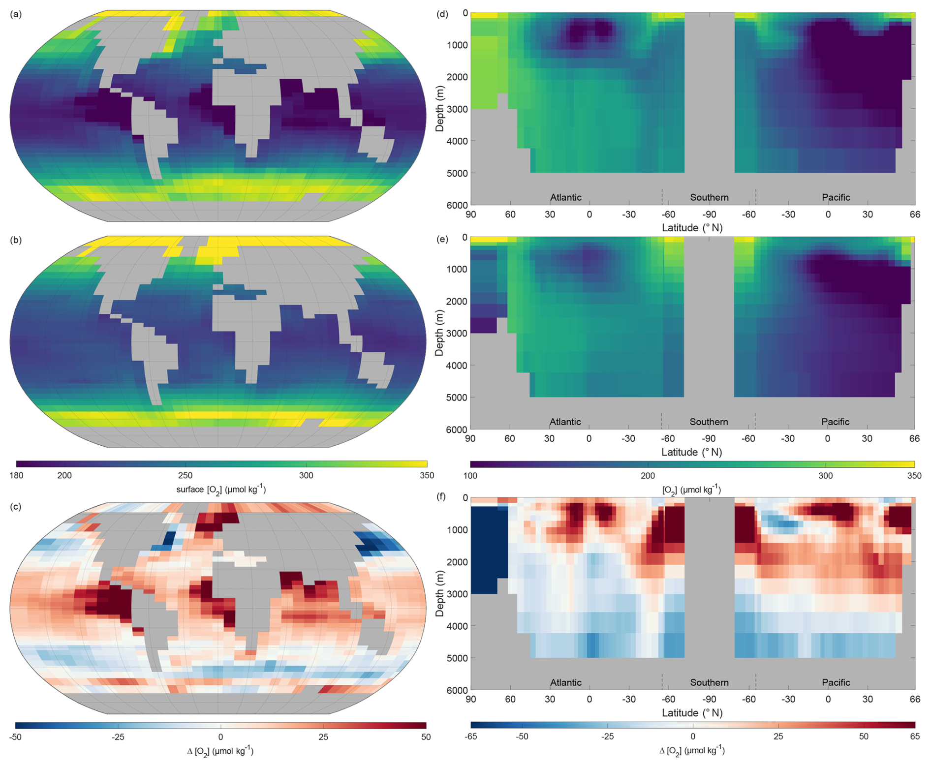
Figure 10 Annual mean global dissolved oxygen ([O₂]). (a) Observed World Ocean Atlas Re-gridded (WOAR) surface [O₂]. (b) NutGEnIE surface [O₂]. (c) Delta surface [O₂] (NutGEnIE – WOAR). (a–c) Based on surface level 0–80.8 m depth level. (d) Observed (WOAR) thermohaline transect zonal mean [O₂]. (e) NutGEnIE thermohaline transect zonal mean [O₂]. (f) Thermohaline transect [O₂] delta (NutGEnIE – WOAR). [O₂] (and difference) in µmol kg⁻¹.

When considering the ocean interior (Fig. 10d–f) and comparing the observed dissolved oxygen concentrations to those of NutGEnIE it is again the case that NutGEnIE largely reflects the observed spatial variations. The Atlantic sector in both the observed and NutGEnIE transects have generally higher dissolved oxygen concentrations than the Pacific Ocean, reflecting the fact the Pacific Ocean contains older water into which there has been greater remineralisation of organic matter. The tongue of AAIW with reduced dissolved oxygen concentrations is evident in both the observed and NutGEnIE transects. In both the observed and NutGEnIE transects the highest dissolved oxygen concentrations are seen towards the surface at high latitudes, that is, the Arctic Ocean, Southern Ocean, and North Pacific. The minimum dissolved oxygen concentrations, approaching 100 µmol kg⁻¹ are in the North Pacific at depths up to 3000 m in both the observed and NutGEnIE transects. However, NutGEnIE does not reflect the observed dissolved oxygen concentrations in the Arctic Ocean at depth well, with concentrations greater than 40 µmol kg⁻¹ below the observed concentrations. In addition, NutGEnIE tends to have higher concentrations of dissolved oxygen (by up to 40 µmol kg⁻¹) in the upper 2000 m of the water column and lower concentrations of dissolved oxygen (by up to 40 µmol kg⁻¹) at greater depths. The mean NutGEnIE annual mean global interior [O₂] is 189 µmol kg⁻¹ with a standard deviation of 55 which compare to WOAR mean and standard deviations of 194 and 65 µmol kg⁻¹ respectively.

3.3.5 Statistical analysis results

Statistical information, such as mean values, have in many cases been provided alongside the results associated with each ocean property; here we summarise the statistical and correlation results.

For all variables there is good agreement between the NutGEnIE and WOAR mean values; all NutGEnIE means are within one standard deviation of the observed WOAR mean. The NutGEnIE datasets are derived from less granular grids and therefore it is understandable that in most cases the associated standard deviations are lower than the WOAR standard deviation. Correlation coefficients between NutGEnIE and WOAR are reassuring with values ranging from 0.76 (surface [O₂]) to 0.97 (surface temperature). In all cases the correlation p-values are zero, indicating strong rejection of the null hypothesis that the NutGEnIE and WOAR datasets are not correlated. Histograms of the NutGEnIE and WOAR datasets for each of the variables in Table 7 also show reassuring similarities (Figs. S26–S35). A graphical representation of the skill of NutGEnIE can by visualised using a Taylor diagram, Fig. 11.

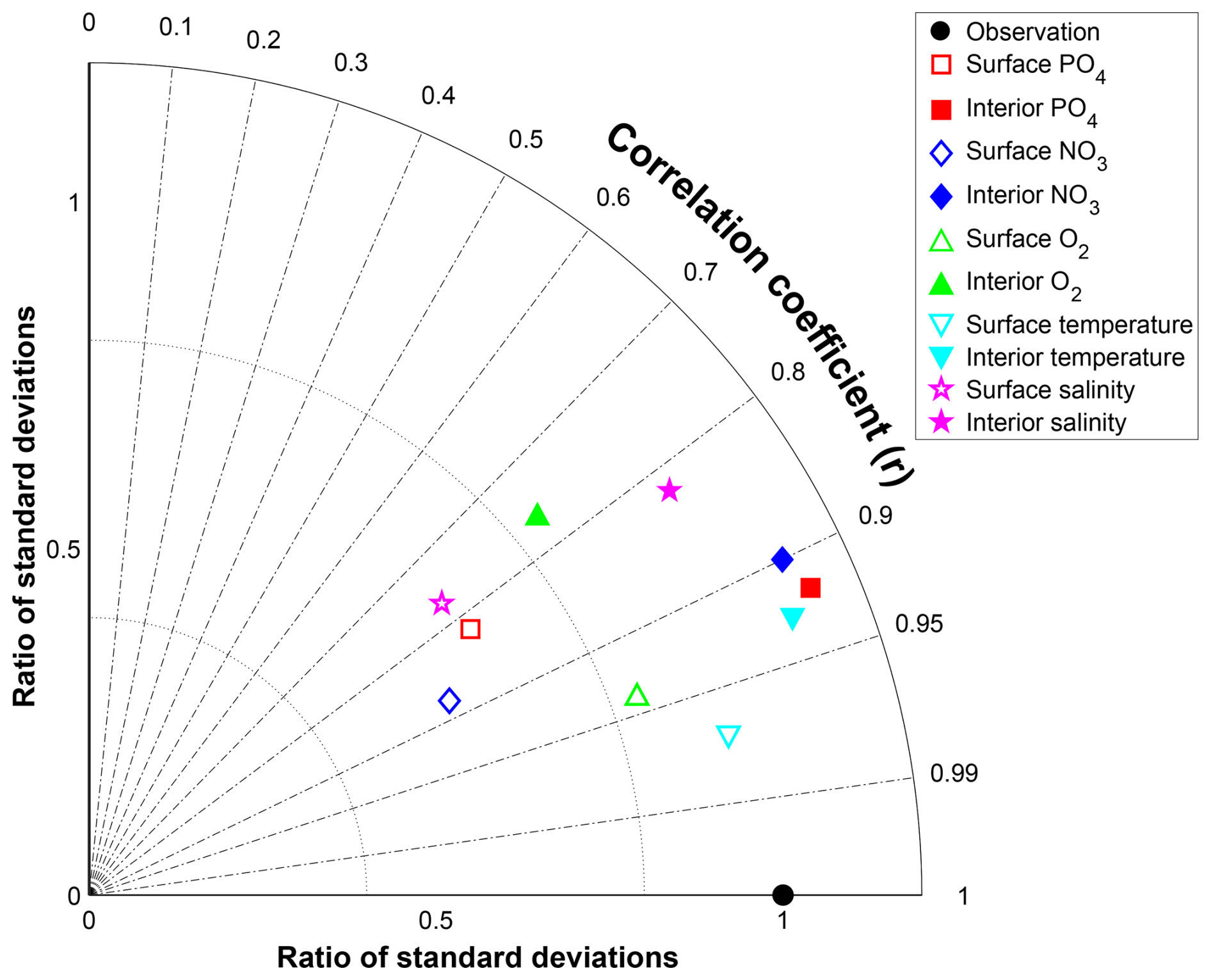
Figure 11 Taylor diagram of NutGEnIE and Observed World Ocean Atlas Re-gridded (WOAR). Showing surface and interior temperature, salinity, [PO${}_{\mathrm{4}}^{\mathrm{3}-}$], [NO${}_{\mathrm{3}}^{-}$] and [O₂]. The RMS error and standard deviations have been normalised by the observed standard deviation of each field before plotting. Therefore, the RMS error and standard deviation indicate the ratio to the observed standard deviation. Angular distance θ is controlled by the correlation coefficient (r), with a correlation of 1 on the x-axis. The diagrams show NutGEnIE results to observation (WOAR) comparisons based on annual average spatial fields.

3.3.6 Rates of PP

It was noted (Sect. 2.2) that NutGEnIE does not explicitly model primary producer (phytoplankton) biomass. Nutrient uptake within the surface layer of NutGEnIE is an output of the model. NutGEnIE nutrient uptake is converted to the units (g C m⁻² d⁻¹) of the Observation-based PP provided by the Oregon State University Ocean Productivity group (Ocean Productivity, 2024) and shown below (Fig. 12). A direct quantitative comparison is not appropriate because NutGEnIE nutrient uptake is equivalent to net ecosystem production whereas the OPR product is net primary production; however, we have provided a qualitative comparison of spatial similarities and differences below.

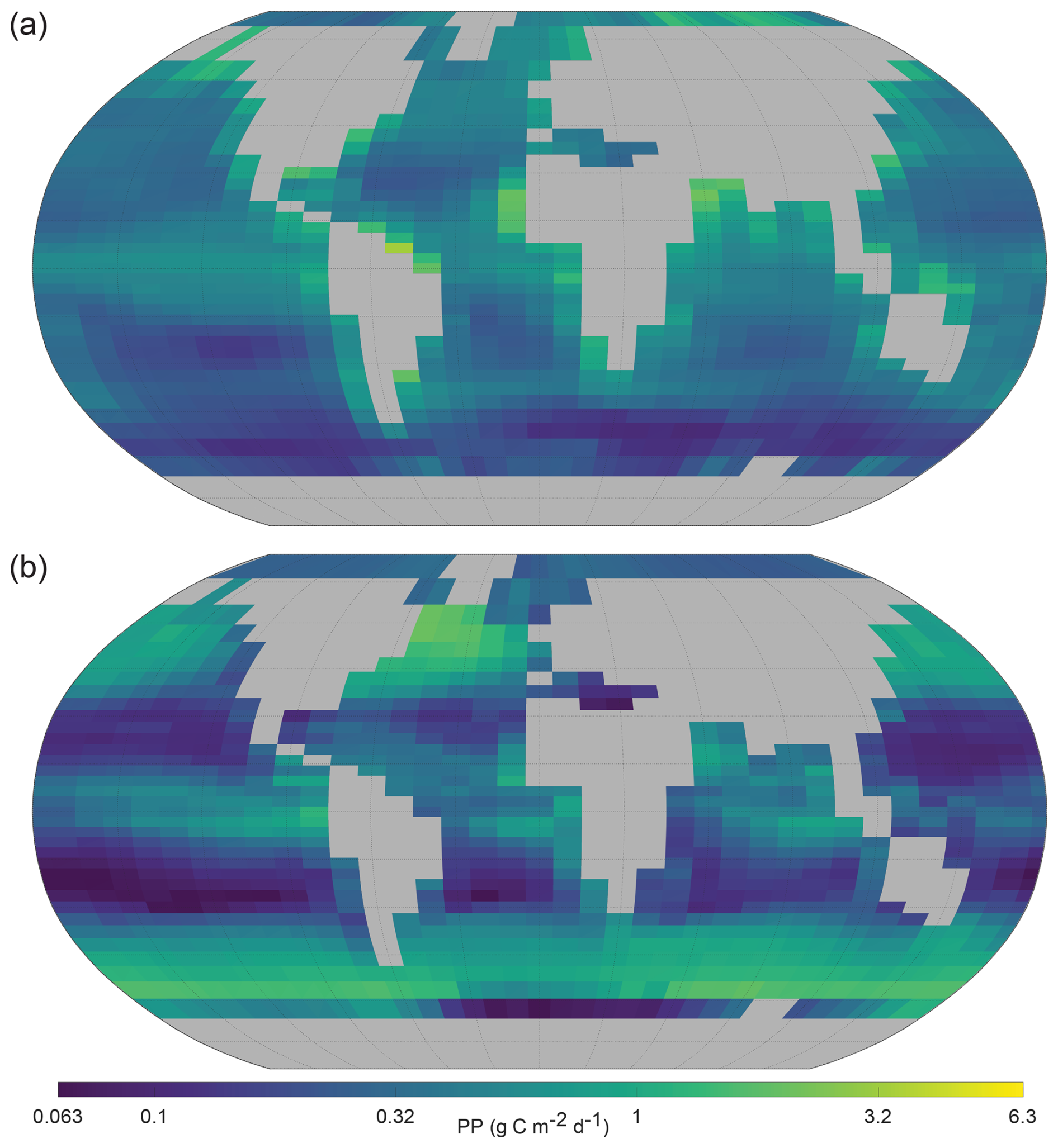
Figure 12 Annual mean global primary production. (a) Oregon State University Ocean Productivity (Ocean Productivity, 2024) re-gridded (OPR). (b) NutGEnIE surface layer nutrient uptake converted to units of g C m⁻² d⁻¹. (a, b) A log (base 10) scale is used and units are g C m⁻² d⁻¹.

Large areas of the oceans away from the continental land masses have low levels of PP and this is reflected in both observations and NutGEnIE (Fig. 12). A figure showing the base Ocean Productivity dataset prior to re-gridding is available in Fig. S36.

PP is enhanced by upwelling, e.g., the equatorial Pacific and Eastern Atlantic, and this is reflected in both observations and NutGEnIE. However, the highest observed rates of PP are seen immediately adjacent to the continental land masses. These elevated observed rates of PP are unable to be reflected accurately by NutGEnIE given the 36×36 spatial resolution. NutGEnIE also overestimates the rate of PP in the North Atlantic in an area south of Greenland and in a band close to 60° S.

3.3.7 Nitrogen cycle processes

The NutGEnIE global mean rate of marine nitrogen fixation is 3.0×10¹² mol N yr⁻¹ which equates to 84 Tg N yr⁻¹, with the majority occurring in the low latitudes, within 30° either side of the equator. The distribution of nitrogen fixation and associated rates in µmol N kg⁻¹ yr⁻¹ can be seen in Fig. 13a. Higher rates of nitrogen fixation in each ocean basin are seen north of the equator than south of the equator. The highest rates of nitrogen fixation (4.0 µmol N kg⁻¹ yr⁻¹) occur between the equator and 15° N in the Atlantic Ocean. A significant area of the Pacific Ocean either side of the equator has minimal or zero rates of nitrogen fixation.

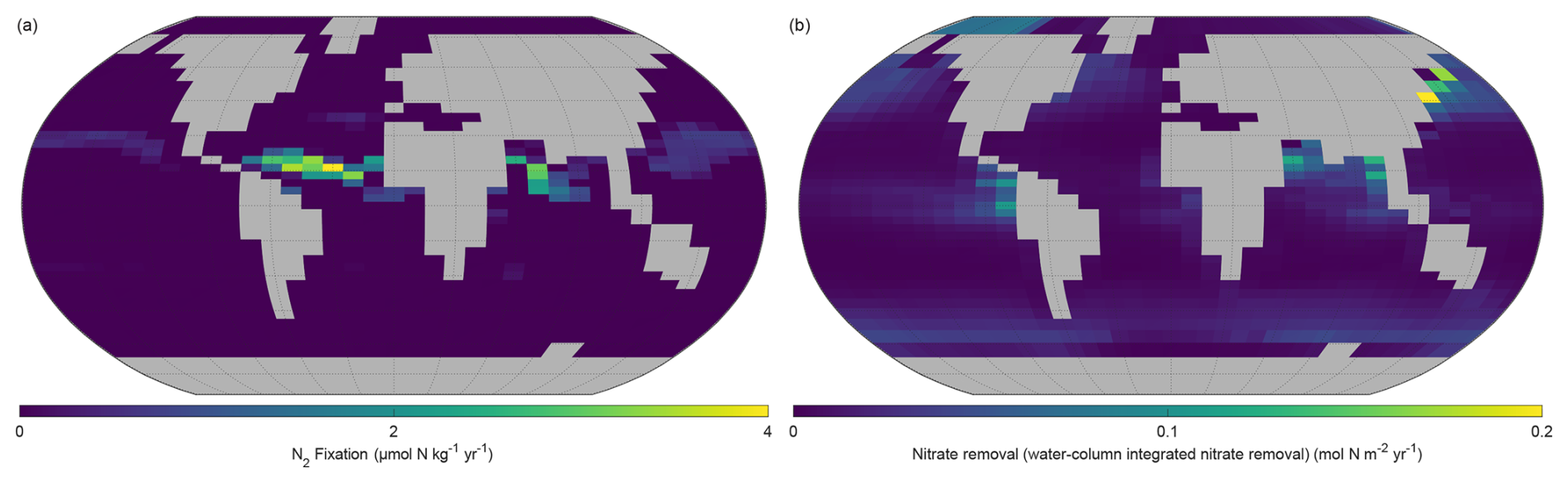
Figure 13 Annual mean distribution of NutGEnIE nitrogen fixation and denitrification. (a) Surface level nitrogen fixation in µmol N kg⁻¹ yr⁻¹. (b) Water column denitrification.

Denitrification can occur throughout the water column, dependant on the consumption of election acceptors in the process of OM remineralisation as outlined in Sect. 2.3.7. In NutGEnIE denitrification occurs via the decomposition of organic matter, when oxygen levels are low, which leads to the use of nitrate as an alternative electron acceptor. This in turn results in the conversion of nitrate to dinitrogen. NutGEnIE water column integrated denitrification is shown in Fig. 13b. The NutGEnIE global mean rate of marine denitrification is 3.2×10¹² mol N yr⁻¹ which equates to 90 Tg N yr⁻¹.

In addition, Nitrogen^* (N^*) (Gruber and Sarmiento, 1997) analysis has been conducted for WOAG and NutGEnIE and provided in Figs. S52 and S53 respectively. The overall trend in N^* for both WOAG and NutGEnIE is that concentrations are highest in the North Atlantic and decrease gradually toward the Pacific. For both WOAG and NutGEnIE this implies a net transport of fixed nitrogen from the Atlantic to the Pacific.

4 Discussion

4.1 Summary

We have presented the features of NutGEnIE and carried out comparisons to datasets based on ocean observations. Focus on nutrient cycles and associated biogeochemical cycles has been vital with NutGEnIE compared to both WOAR (phosphate, nitrate and dissolved oxygen) and GEOTRACES (iron) datasets. In addition, the WOA provides temperature and salinity datasets that have been compared with NutGEnIE so give confidence that the fundamental physical properties are being well represented. NutGEnIE has also been qualitatively compared against ocean productivity data from the Oregon State University Ocean Productivity group. For each attribute the comparisons have shown that NutGEnIE is an effective representation rather than a perfect replication of the oceans which would be unrealistic.

The NutGEnIE steady state nutrient global inventories (Fig. 4) are well aligned to ocean estimates; this is also evident in the comparisons of interior nutrient concentrations. Fluxes associated with each NutGEnIE nutrient cycle, considering the simplified cycles, are close to literature estimates of ocean nutrient budgets. NutGEnIE residence times (phosphate ∼40 000 years, nitrate ∼6000 years and iron < 1000 years) are of the expected order of magnitude, although iron is slightly higher than global ocean estimates of tens to hundreds years (Delaney, 1998; Gruber, 2004; Hayes et al., 2018). This supports the conclusion that NutGEnIE nutrient cycles as configured here are a reasonably accurate representation of the oceans.

The mechanisms that maintain NutGEnIE ocean nutrient concentrations are pertinent to the intended investigations and, therefore, significant discrepancies would be worrying. Annual mean concentrations of phosphate and nitrate both compare successfully to the WOAR. Those comparisons have considered both the areas with first order impact to ocean PP, that is, the surface ocean and the ocean interior that has longer term impact on PP in terms of nutrient replenishment. It is noted that the mean NutGEnIE annual mean global surface [NO${}_{\mathrm{3}}^{-}$] is 3.0 µmol kg⁻¹ compared to a WOAR value of 6.0 µmol kg⁻¹. NutGEnIE agrees well with WOAR across most of the surface ocean with the discrepancy mainly relating to the Southern Ocean and northern Pacific Ocean. This bias is deemed acceptable as the configuration results in rates of PP, spatial variation of nutrient limitation (Sect. 4.2), nitrogen cycle dynamics and other properties that have good validation results. Differences in both nutrients' concentrations have been identified and noted; however, there are no significant flaws in NutGEnIE distributions related to phosphate and nitrate.

NutGEnIE's global mean rate of marine nitrogen fixation and denitrification are 84 and 90 Tg N yr⁻¹ respectively these are both lower than ocean estimates, for example, these NutGEnIE global rates are 67 % and 52 % of the Gruber and Sarmiento (1997) estimates. The spatial distributions of NutGEnIE nitrogen fixation and denitrification are encouraging and alongside N^* analysis (Figs. S52 and S53) indicate that NutGEnIE largely represents the nitrogen fixation and denitrification processes well. Apparent Oxygen Utilisation (AOU) analysis can give an insight into biological processes, primarily through respiration/remineralisation, that consume oxygen see Figs. S50 and S51. The similarity of the WOAR and NutGEnIE AOU transects give additional reassurance that the rate of export and subsequent remineralisation processes in NutGEnIE are realistic.

In summary, the validation of NutGEnIE results against ocean observations suggest that NutGEnIE represents the ocean successfully. In particular, the representation of nutrient concentrations give confidence that NutGEnIE will be suitable for the intended study of long-term influence of nutrients on oceanic PP. There are, however, aspects of NutGEnIE as configured here that do not represent reality as successfully and these are noted below. The representation of the Artic Ocean has highlighted discrepancies relating to temperature, salinity, and dissolved oxygen below the surface. In general, NutGEnIE nutrient concentrations in the upper 1000 m of the northern Pacific Ocean are lower than observed concentrations, NutGEnIE biases in this area also exist for temperature, dissolved oxygen and AOU. NutGEnIE overestimates PP in an area of the North Atlantic close to Greenland and a band close to 60° S. Whilst these discrepancies are noted, the ability of NutGEnIE to successfully represent Earth's oceans and processes indicate that NutGEnIE will be useful for the future investigations into the long-term influence of nutrients on oceanic primary production.

4.2 Spatial variation of limitations

The comparisons to ocean observations detailed in the results have not considered the limiting factors that act to control PP. Here, we briefly review those limiting factors and in particular the spatial variation of nutrient limitation to ensure that NutGEnIE is realistic as these aspects will be vital in the proposed investigations of the ULN.

The nature of light and temperature limitations are such that they exert the greatest restriction on nutrient uptake in the higher latitudes. The comparative limitations of nutrient uptake by light, temperature, and nutrient supply are shown in Fig. 14 for both other phytoplankton and diazotrophs. For both phytoplankton classes a combination of light, temperature, and nutrient supply limit nutrient uptake in the high latitudes. The nutrient uptake at low and mid latitudes is controlled by nutrient availability. The spatial variability of nutrient limitation is shown in Fig. 15 that displays the PLN for each phytoplankton class.

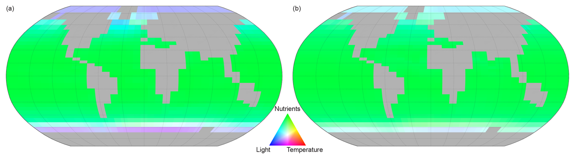
Figure 14 Spatial variation of the limiting factor for nutrient uptake, (a proxy for phytoplankton growth in NutGEnIE). For (a) other phytoplankton and (b) diazotrophs. Red = temperature limitation, green = Nutrient limitation, blue = light limitation.

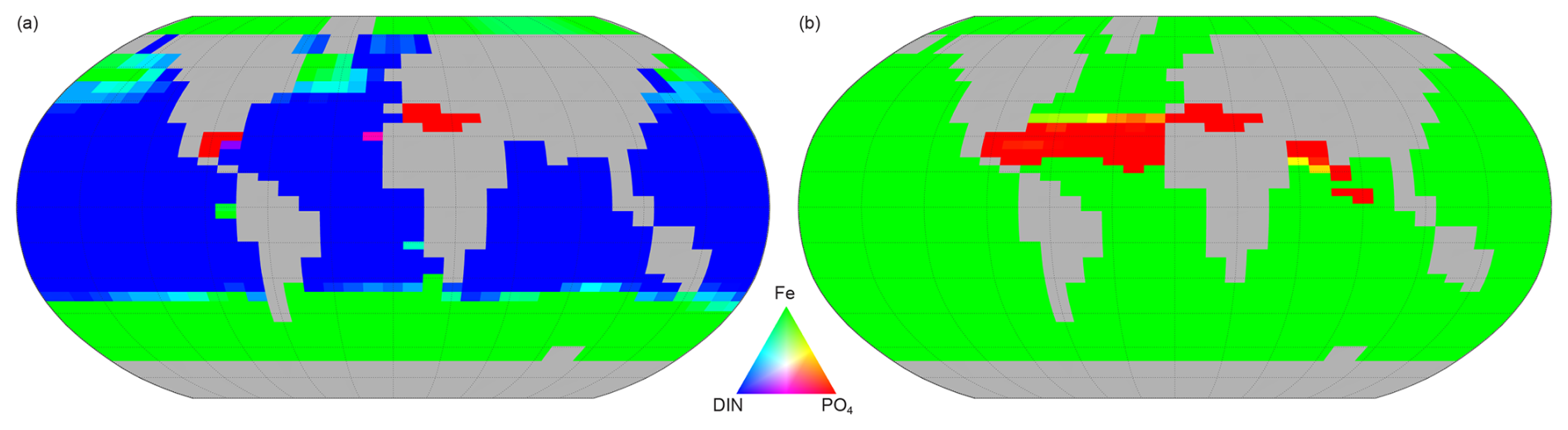
Figure 15 Spatial variation of the limiting factor for nutrient uptake (proxy for phytoplankton growth in NutGEnIE). (a) Other phytoplankton, red = PO${}_{\mathrm{4}}^{\mathrm{3}-}$ limitation, green = Fe limitation, blue = DIN limitation. (b) Diazotrophs (are not limited by DIN as nitrogen is considered freely available via nitrogen fixation) red = PO${}_{\mathrm{4}}^{\mathrm{3}-}$ limitation, green = Fe limitation.

Figure 14 facilitates the representation of the three limiting factors on a single figure, however, the colours used are not favourable to readers with colour vision deficiencies. Figures showing individual limiting factors are available in supplementary information Figs. S37–S45.

Other phytoplankton nutrient uptake is limited by a combination of nutrients. PO${}_{\mathrm{4}}^{\mathrm{3}-}$ is the PLN in 1 % of the surface ocean, DIN is the PLN for 71 % and Fe limiting in the remaining 28 %. PO${}_{\mathrm{4}}^{\mathrm{3}-}$ limitation is restricted to the Mediterranean Sea and a small area of the Caribbean. The areas where Fe acts as the PLN are the Southern Ocean, south of 40° S, and north of 40° N in both the Pacific and Atlantic Oceans.

Nutrient uptake by diazotrophs will only be limited by either Fe or PO${}_{\mathrm{4}}^{\mathrm{3}-}$ (dinitrogen is freely available for nitrogen fixation). In this configuration of NutGEnIE, Fe is the PLN for diazotrophs across 93 % of the surface ocean, with PO${}_{\mathrm{4}}^{\mathrm{3}-}$ being the PLN in the remaining 7 %. The areas where PO${}_{\mathrm{4}}^{\mathrm{3}-}$ acts as the PLN for diazotrophs are restricted to the northern hemisphere and are the Atlantic Ocean from 15 to 40° N; the Mediterranean Sea; and a section of the Indian Ocean from the equator to 30° N.

Figure 15 shows the limiting nutrient in each surface cell, in addition, supplementary figures providing the calculated limiting value for each nutrient are available in Figs. S46–S49.

The additional diagnostic tools that have allowed the spatial variations in the limiting factors (Fig. 14) and PLN (Fig. 15) to be visualised are also reassuring. Given the proposed use of this configuration of NutGEnIE to investigate long term nutrient limitation of PP it is important that the spatial variations are realistic. Mahowald et al. (2017) (see Fig. 3 therein) produced schematic distributions of factor and nutrient limitation for differing phytoplankton classes. The results of NutGEnIE compare well to the schematics of Mahowald et al. (2017). In addition, Browning and Moore (2023) (see Fig. 1 therein) carried out a global analysis of phytoplankton nutrient limitation, summarising over 150 experiments identifying the PLN. NutGEnIE (Fig. 15a) is aligned well with the summary of Browning and Moore (2023) although, two discrepancies are noteworthy. Firstly, NutGEnIE identifies phosphorus as the PLN in the Mediterranean Sea and a small area of the Caribbean, whereas in these areas Browning and Moore (2023) identify fixed nitrogen as the PLN with co- or serial phosphorus limitation. Secondly, in NutGEnIE the area of the equatorial Pacific Ocean where iron is identified as the PLN is somewhat smaller than that identified by Browning and Moore (2023).

4.3 The ULN and future work

The flexibility NutGEnIE model allows for different continental configurations alongside varying atmospheric conditions that would allow investigations of the impact of nutrient supply on PP in paleo-worlds scenarios (e.g. Wilson et al., 2018). NutGEnIE would also facilitate experiments or simulations that consider differing nutrient input fluxes and or residence times or differing nutrient requirements of phytoplankton.

Earlier we considered the distinction between the PLN and the ULN for oceanic PP. The limitations of previous work to identify the ULN have also been discussed along with required characteristic of any model intended to investigate the ULN (Sect. 1.3). Aspects relating to the biogeochemical cycles of NutGEnIE and the ability to represent reality are summarised above. However, two additional critical aspects when investigating the ULN were detailed in Sect. 1.3, the importance of an open system model and for model run times to considerably exceed the residence times of all nutrients. The open nutrient cycles have been detailed in Sect. 2.3 and NutGEnIE model runs up to 500 kyr are feasible. NutGEnIE compute times are approximately 10 000 simulation years per day. Phytoplankton stoichiometric requirements used in NutGEnIE are set via parameters, Table 2. These stoichiometric requirements are known to vary (e.g. King et al., 2012), the values of the associated parameters should be considered and potentially the subject of sensitivity analysis during the ULN investigations.

Comparisons between NutGEnIE and real ocean data (encompassing physical processes, nutrients, and BGC processes) have been made and in each case the comparisons indicate that as configured here NutGEnIE is a suitable tool for the study of the ULN question. The proposed use here is to consider the limiting influences that nutrients have on ocean PP over the long term, therefore realistic surface nutrient concentrations are vital. Surface nutrient concentrations are influenced by both physical and BGC processes, hence the relevance in reviewing those aspects. The NutGEnIE model as configured here is representing Earth's oceans (area of $\sim \mathrm{361}\times {\mathrm{10}}^{\mathrm{12}}$ m², volume of $\sim \mathrm{135}\times {\mathrm{10}}^{\mathrm{16}}$ m³) by a 36×36 grid with 16 depth levels. This level of abstraction will not be able to accurately reproduce the complexities of ocean processes; it is however important that the most relevant processes are included with sufficient detail. Therefore, we have focused on whether a good representation rather than a perfect replication of the oceans has been obtained.

The CLIMBER-X model has several similarities to NutGEnIE (Willeit et al., 2023) and could also, if modified, be used to investigate the ULN for oceanic PP. CLIMBER-X has a higher resolution (5°×5°) than NutGEnIE with 23 depth levels as opposed to the 16 of NutGEnIE (Willeit et al., 2022). CLIMBER-X represents phytoplankton and zooplankton as tracers (Willeit et al., 2023) as opposed to the nutrient uptake approach of NutGEnIE. However, diazotrophs are disabled by default in CLIMBER-X and N₂ fixation is represented by a diagnostic formulation (Willeit et al., 2023). CLIMBER-X also has a closed phosphorus budget and the iron ligand association constant is fixed across the water column (Willeit et al., 2023). It would be interesting to compare results from the two models if CLIMBER-X were to be given explicit diazotrophs, open nutrient cycles and depth-variable ligand behaviour. We suggest that the novel aspects of NutGEnIE (in particular the concurrent use of three open nutrient cycles and the dynamic ligand binding mechanism with stronger binding in the upper water column) presented here make it an appropriate option for investigating the ULN.

5 Conclusions

Our motivation has been to create a model, NutGEnIE, that can be used to investigate the ULN for oceanic PP focusing on the nitrogen, phosphorus and iron cycles. A key development has been to ensure that the modelled iron cycle is realistic by including a dynamic ligand mechanism. The novel aspect that each nutrient cycle is open with the ability for inventories to vary over time is of particular importance in the investigation of the ULN. The introduced surface fluxes of PO${}_{\mathrm{4}}^{\mathrm{3}-}$ and NO${}_{\mathrm{3}}^{-}$, seafloor flux of Fe and existing dust supply of Fe provide mechanisms that will allow fertilisation simulations to investigate the ULN.

We have conducted an extensive validation of biogeochemical aspects of NutGEnIE by comparing pertinent tracers to real ocean observations in both surface waters and the ocean interior. This review has highlighted areas of discrepancies but, more importantly, supports the fact that, overall, NutGEnIE reflects the processes and state of the ocean with a good degree of accuracy. Statistical comparisons of NutGEnIE properties to ocean observation have provided evidence that this configuration of NutGEnIE is suitable to conduct the planned nutrient limitation analysis. We believe these validations support the suggestion that NutGEnIE can be used for that purpose and to investigate other questions related to the role of nutrients on oceanic biogeochemical processes.

The primary motivation behind establishing this configuration is to analyse the long-term influence of nutrient limitation on oceanic PP and we conclude that NutGEnIE, as configured and evaluated here, can support such a study. This configuration of NutGEnIE can also be useful in the analysis of the dynamics of nutrient supply and oceanic PP in past, present or future scenarios.