Evaluation of ozone and its precursors using the Multi-Scale Infrastructure for Chemistry and Aerosols Version 0 (MUSICAv0) during the Michigan–Ontario Ozone Source Experiment (MOOSE)

Surface ozone (O₃) in Southeast Michigan (SEMI) often exceeds US National Ambient Air Quality Standards, posing risks to human health and agroecosystems. SEMI, a relatively small region in the state of Michigan, contains most of the state's anthropogenic emission sources and more than half of the state's population and is also prone to long-range and transboundary pollutant transport. Here, we explore the distribution of O₃ and its precursors, such as nitrogen oxides (NO_x) and volatile organic compounds, over SEMI during the summer of 2021 using the chemistry–climate model MUSICAv0 (Multi-Scale Infrastructure for Chemistry and Aerosols Version 0). Using the regional refinement capabilities of MUSICAv0, we create a custom grid over the state of Michigan of $\mathrm{1}/\mathrm{16}$° (∼ 7 km) to better understand the local-scale impacts of chemical and dynamic complexity in SEMI and compare it with a grid with $\mathrm{1}/\mathrm{8}$° (∼ 14 km) resolution over the contiguous United States. Model simulations are evaluated using a comprehensive suite of observations from Phase I of the Michigan–Ontario Ozone Source Experiment (MOOSE) field campaign. MUSICAv0, with its higher horizontal grid resolution, showed excellent skill in capturing peak O₃ concentrations but showed larger variation in the simulation of O₃ precursors (e.g., NO_x, HCHO, isoprene). In addition, we implement a diurnal cycle for anthropogenic nitric oxide (NO) emissions, which is generally not included in global models. As a result, modeled nighttime O₃ is improved because of lower NO_x concentrations during the night. This work shows that when conceptualizing models in urban regions, it is important to consider a combination of high horizontal resolution and the diurnal cycle of emissions, as they can have important implications for the simulation of secondary air pollutants.

1 Introduction

Air pollution can significantly impact air quality (Akimoto, 2003; Fiore et al., 2002; Jacob et al., 1993), human health (Anenberg et al., 2019; Huang et al., 2020; Lelieveld et al., 2015), and climate change (Monks et al., 2015; Ramanathan et al., 2002; Ramanathan and Feng, 2008; Unger et al., 2010). Although air quality in the United States has substantially improved since the implementation of the Clean Air Act of 1990, tropospheric ozone (O₃) still poses a challenge to many regions in the United States (Cooper et al., 2014, 2015; Jaffe and Ray, 2007). O₃, a secondary air pollutant formed through the photochemical interactions between its gas-phase precursors, i.e., nitrogen oxides (NO_x= NO + NO₂) and volatile organic compounds (VOCs), often exceeds allowable limits for O₃ established by the National Ambient Air Quality Standards (NAAQS) set by the United States Environmental Protection Agency (US EPA) (i.e., a maximum daily 8 h average (MDA8) of 70 ppbv or less) in various US cities, despite significant reductions in its precursor species.

Southeast Michigan (SEMI) has often been classified as a non-attainment area for O₃ (US Environmental Protection Agency, 2021). SEMI has experienced historically high levels of air pollution from being heavily concentrated with industry (e.g., coal-fired power plants, steel and cement facilities, petroleum refineries, and incinerators) and is subject to various mobile emissions sources due to its proximity to highways and the US–Canada ports-of-entry (in Detroit and Port Huron). Elevated O₃ levels have been associated with a variety of negative impacts to human health, agriculture, and the natural environment, which include premature deaths attributable to respiratory and cardiovascular diseases (Sicard et al., 2018), impacts to crop yields resulting from reduced photosynthesis (Fuhrer et al., 1997; Wortman and Lovell, 2013), and reduced visibility due to photochemical smog. The Michigan–Ontario Ozone Source Experiment (MOOSE) (Olaguer et al., 2023) was carried out to define potential O₃ attainment strategies in SEMI and better understand what contributes to O₃ exceedances in the region. It was a multi-institution (e.g., Michigan Department of Environment, Great Lakes, and Energy (EGLE), Environment Climate Change Canada (ECCC), Ontario Ministry of Environment, Conservation, and Parks (MECP), and university partners) campaign that was carried out in two phases: Phase I (24 May to 30 June 2021) and Phase II (6–28 June 2022). The MOOSE observations included a mobile lab with detailed measurements of ozone and its precursors, ground-based remote sensors (i.e., Pandora), and an airborne remote sensor (i.e., GEO-CAPE Airborne Simulator). Previous studies in Michigan have mainly investigated the impact of lake breezes on air quality (Abdi-Oskouei et al., 2020; Acdan et al., 2023; Brook et al., 2013; Dye et al., 1995; Hanna and Chang, 1995; Stanier et al., 2021; Vermeuel et al., 2019) and the connections between human health adversities and air pollution (Cassidy-Bushrow et al., 2020; Lemke et al., 2014), with little attention focused on O₃ atmospheric chemistry in SEMI. Xiong et al (2023) was the first to use a combination of MOOSE campaign measurements in 2021 and box modeling to investigate O₃ formation regimes in SEMI and found that summertime O₃ is limited by VOC emissions but pointed to uncertainties due to the small number of days used for the analysis. Because the spatial distribution of O₃ is dependent on precursor emissions, location, and meteorology, local O₃ production and loss in SEMI may be largely different compared to other regions.

Models provide credible, process-based mathematical representations of chemistry–climate interactions in the atmosphere (Brasseur and Jacob, 2017). O₃ biases have been identified in various global chemistry–climate models, with suggestions for improvements, such as better representation in temperature, anthropogenic emission inventories, and deposition (Schwantes et al., 2022). However, in many of these cases, the global models were not being run at horizontal and vertical resolutions fine enough to simulate ozone production and loss accurately (Schwantes et al., 2022). Although current models are efficient in reproducing rural pollutant concentrations, surface O₃ bias persists, which can be attributable to a coarse (> 100 km) grid's ineffectiveness at reproducing urban sources and transport (Jo et al., 2013; Monks et al., 2015). The large grid cells in coarse grids artificially dilute local emissions of O₃ precursors, imported pollution plumes, and topography, which can alter abundance and mixing at the surface (Monks et al., 2015). There have been advancements in the use of high horizontal grid resolutions (1–28 km), which have the potential to produce more realistic simulations of O₃ production and loss. MUSICA (Multi-Scale Infrastructure for Chemistry and Aerosols) is a state-of-the-science unified modeling framework, allowing for seamless global and regional simulation within one model with consistent dynamics and chemistry (Pfister et al., 2020). The initial implementation of MUSICA (MUSICAv0) is a configuration of CAM-chem (the Community Atmosphere Model with chemistry) available in the Community Earth System Model Version 2 (CESM2; Danabasoglu et al., 2020) using the spectral element (SE) dynamical core, allowing for regional refinement. Several studies have taken advantage of MUSICAv0's regional refinement capabilities using custom grid applications. Schwantes et al. (2022) evaluated horizontal resolution and chemistry at varying scales (∼ 111 and ∼ 14 km) over the Southeastern US and found that O₃ was better simulated over urban regions, particularly using the ∼ 14 km grid and updated isoprene and terpene chemistry. Tang et al. (2022) included plume rise and a diurnal cycle of fire emissions in MUSICAv0, using the standard ∼ 14 km resolution over the contiguous US (CONUS), and found that this addition improved MUSICAv0 simulations compared with observations. Tang et al. (2023) developed a custom grid over Africa at ∼ 28 km in MUSICAv0, compared it to the regional model WRF-Chem (Weather Research Forecast with Chemistry), and found that MUSICAv0 performance was comparable to that of WRF-Chem when comparing to satellite and surface measurements of O₃ and carbon monoxide (CO). Jo et al. (2023) constructed two global (∼ 112, ∼ 56 km) and two regional (∼ 14, ∼ 7 km) refinement grids over South Korea for use in MUSICAv0 and found that grid resolution can heavily impact model evaluation near the surface, in particular within urban regions, as well as strongly affect the oxidation of VOCs. Lichtig et al. (2024) used a custom grid over South America with a resolution of ∼ 28 km to quantify the local and long-range origins of CO in the region. Edwards et al. (2024) used MUSICAv0, along with the Geostationary Environment Monitoring Spectrometer (GEMS), to study NO_x over Northeast Asia and Seoul, South Korea, to distinguish different emission sources. As can be noted from previous work, custom grids have been used to understand an extensive range of atmospheric physical and chemical processes.

In this study, we created a custom regional refinement grid over the state of Michigan in the United States with a horizontal resolution of $\mathrm{1}/\mathrm{16}$° (∼ 7 km) and compared it to the standard MUSICAv0 $\mathrm{1}/\mathrm{8}$° (∼ 14 km) grid over CONUS. We used the Community Mesh Generation Toolkit, which is available to the community and provides the necessary tools for defining a high-resolution grid mesh (i.e., generating input files). A sector-based diurnal cycle was applied to anthropogenic nitric oxide (NO) emissions and was included for each resolution (Crippa et al., 2018; Jo et al., 2023). In total, four simulations were run during Phase I of the MOOSE campaign, which included a variety of high-resolution measurements used for model evaluation. This work focuses on evaluating the model simulations with measurements from MOOSE, the differences between the regional refinement grids, and changes that result from the application of the diurnal cycle for anthropogenic NO emissions.

2 Methodology

2.1 Model description

2.1.1 Model overview

Simulations with regional refinement over CONUS and Michigan were conducted using MUSICAv0. The model uses the spectral element (SE) dynamical core, an unstructured grid mesh based on a cubed sphere, allowing for regional refinement (Lauritzen et al., 2018). The standard resolution for MUSICAv0 is the uniform ne30x8 CONUS grid (hereafter referred to as ne30x8), which is 1° (∼ 111 km) over most of the globe with a mesh refinement of $\mathrm{1}/\mathrm{8}$° (∼ 14 km) over CONUS and 32 vertical layers (model top of approximately 40 km). The ne30x8 grid uses a physical/chemical time step of 225 s. Simulations use the MOZART-TS2 (Model of OZone And Related chemical Tracers, troposphere-stratosphere v2) chemical mechanism, which expands a comprehensive representation of tropospheric and stratospheric chemistry (MOZART-TS1, Emmons et al., 2020) with more detailed gas-phase chemistry for isoprene and terpene species (Schwantes et al., 2020), aerosol microphysics using the 4-mode Modal Aerosol Module (MAM4) (Liu et al., 2016b), and the simplified Volatility Basis Set (VBS) scheme (Tilmes et al., 2019). MAM4 assists in simulating the spatial distribution of aerosols to include type, optical depth, number, and size distributions, while the VBS scheme allows model users to better simulate secondary organic aerosols (SOAs) in urban areas through NO_x-dependent SOA formation (Jo et al., 2021).

Four simulations are presented in this study and were conducted from April to August of 2021, using the month of April as a spin-up, with a particular focus on Michigan. Initial conditions for the chemical species in the simulations were generated based on an April 2021 restart file from a 1° finite volume CAM-chem run using the MOZART-TS1 chemistry and regridded to the respective SE grids used here. Although the initial condition file was based on the MOZART-TS1 chemistry and the additional species in MOZART-TS2 were initiated from zero, the majority of these species are short-lived and equilibrate quickly within the 1-month spin-up period. Meteorological fields (e.g., temperature, horizontal, and vertical winds) are nudged toward meteorological reanalysis data from MERRA-2 (Modern-Era Retrospective Analysis for Research and Applications, Version 2) (Gelaro et al., 2017) and interpolated to the resolution of the SE grids. For this study, nudging was not applied within the state of Michigan (horizontal center of the nudging window: 43° N, 275° W) because the original resolution of MERRA-2 is coarser than the spectral element grids used, which could influence meteorological field calculations at finer resolutions (Jo et al., 2023).

2.1.2 Regional refinement over Michigan

To better study the distribution of O₃ in SEMI, an SE grid was created over the state of Michigan using the Community Mesh Generation Toolkit (University Corporation for Atmospheric Research, 2025). Using the Variable Resolution Mesh Editor, the cubed sphere was rotated to have a face centered over Michigan. The 1° (ne30) base grid was further refined over Michigan to a $\mathrm{1}/\mathrm{16}$° (ne30x16) grid, or approximately 7 km. The $\mathrm{1}/\mathrm{16}$° grid then transitions into a $\mathrm{1}/\mathrm{8}$° (∼ 14 km) horizontal resolution over the remainder of EPA Region 5 (which includes Wisconsin, Illinois, Indiana, Ohio, and parts of Minnesota) and finally into the 1° (∼ 111 km) horizontal resolution over the rest of the globe. The finer-resolution grid over Michigan will, hereafter, be referred to as ne30x16. To create a smooth transition between the finer and coarser resolutions, a halo was created around Michigan and EPA Region 5, respectively, to mitigate potential errors associated with the varying resolution changes. The ne30x8 and ne30x16 grids are shown in Fig. 1a and b, respectively.

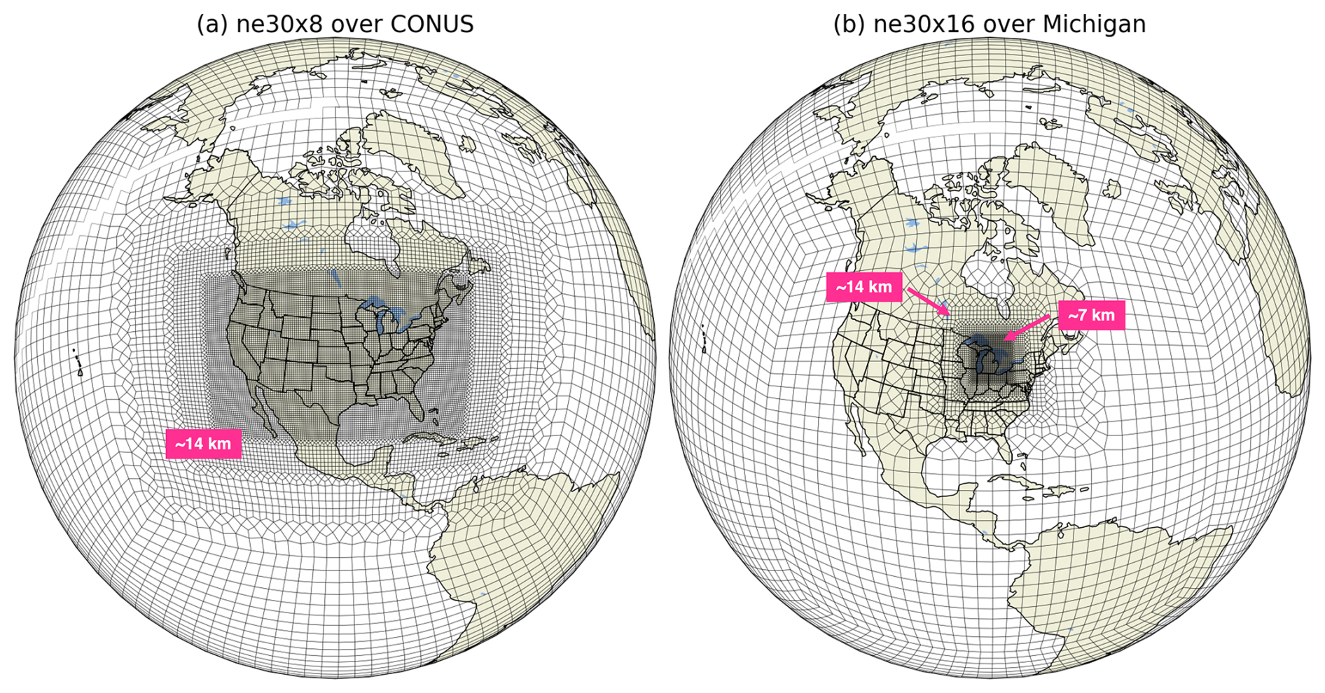
Figure 1 The variable resolution mesh grids used for the MUSICAv0 simulations in this study. (a) The ne30x8 grid and standard resolution of MUSICAv0, which is $\mathrm{1}/\mathrm{8}$° (∼ 14 km) over the contiguous United States (CONUS) and 1° (∼ 100 km) for the rest of the globe, and (b) the ne30x16 grid with regional refinement over Michigan of $\mathrm{1}/\mathrm{16}$° (∼ 7 km), $\mathrm{1}/\mathrm{8}$° over the majority of EPA Region 5 (which includes Wisconsin, Illinois, Indiana, Ohio, and parts of Minnesota), and 1° for the rest of the globe.

MUSICAv0 simulations using the ne30x8 and ne30x16 horizontal resolutions were run with identical dynamical cores, physics packages, and chemistry settings, but differences arise due to the different horizontal resolutions and computational time steps. The physics time step specifies the number of times per model-day that the physics package is called. It also defines many other time steps in the model through the division of the physics time step by some integer. Scaling physics and dynamics time steps in proportion to grid spacing is necessary for model stability. Physics and dynamic time steps for the ne30x8 and ne30x16 grids are based on recommendations within the Community Mesh Generation Toolkit. Physics time steps for both the ne30x8 and ne30x16 grids were set to 225 s, and dynamic time steps, to 37.5 and 18.75 s, respectively. The computational cost for each resolution varies based on the configuration, saved output, and computational systems used. At identical model configurations, the ne30x8 and ne30x16 resolutions have computational costs of ∼ 26 000 and ∼ 22 000 core hours per simulated month, respectively. The finer-resolution grid is about 17 % more cost-efficient because it has 80 138 grid points as opposed to 174 098 in the CONUS ne30x8 grid. Configurations similar to the Michigan grid could be beneficial for local-scale studies that do not require fine resolution over an entire continent.

2.1.3 Emissions

MUSICAv0 has made great advances with emission dataset implementation for high horizontal grid resolutions (Schwantes et al., 2022). The model is coupled with the Community Land Model Version 5 (CLM5) (Lawrence et al., 2019), which includes the Model of Emissions of Gases and Aerosols from Nature Version 2.1 (MEGANv2.1) algorithm to calculate biogenic emissions from vegetation (Guenther et al., 2012). Biogenic VOCs (BVOCs) represent more than 80 % of the total global VOCs present in the atmosphere (Guenther et al., 1995), where isoprene alone makes up about half (Guenther et al., 2012). For this study, the specified phenology (SP) configurations of CLM are used, where MEGANv2.1 calculates biogenic emission rates in CLM based on plant functional type (PFT) distributions and the leaf area index (LAI) obtained from MODIS (Moderate Resolution Imaging Spectroradiometer) (Guenther et al., 2012). Because biogenic emissions are calculated online in the model, they can vary based on horizontal resolution due to improved simulated meteorological fields (e.g., temperature) from resolving topography (Jo et al., 2023).

The anthropogenic and biomass burning emissions are conservatively regridded offline using the first-order conservative method (Jones, 1999) to the corresponding horizontal grid resolutions (i.e., ∼ 14 and ∼ 7 km) used in the MUSICAv0 simulations. These regridded emissions better resolve sources and result in less artificial dilution of concentrated emissions with surrounding lower values (Schwantes et al., 2022). Emission inventory estimates are generally developed based on activity data availability for various sectors (e.g., transportation, industry, agriculture, shipping) and emission factors derived from the mass emitted per activity unit (Monks et al., 2015). Global anthropogenic emissions are from the Copernicus Atmospheric Monitoring Service Version 5.1 (CAMS-GLOB-ANTv5.1), which are monthly emissions based on EDGARv5 (Emissions Database for Global Atmospheric Research Version 5: https://edgar.jrc.ec.europa.eu/dataset_ghg50, last access: 15 September 2025) until 2015 and then assumed until 2021 based on trends calculated from CEDSv2 (Community Emissions Data System Version 2; Hoesly et al., 2018) (Elguindi et al., 2020). CAMS-GLOB-ANTv5.1 is available at a 0.1° × 0.1° spatial resolution, which is comparable to the finest resolutions of the model grids. Table 1 shows the anthropogenic emissions of select species for SEMI in comparison to the rest of the state of Michigan to demonstrate the magnitude of SEMI emissions being represented in the model. It is important to recognize that for many of the anthropogenic emissions listed in Table 1, SEMI makes up about a third of Michigan's total anthropogenic emissions. CAMS-GLOB-AIRv2.1 provides aircraft emissions from the aviation emission inventory (Version 2.1) at a spatial resolution of 0.5° × 0.5° (Granier et al., 2019). Biomass burning emissions are available through the Quick Fire Emissions Dataset (QFED) (Darmenov and da Silva, 2015) with emission factors for aerosols and trace gases from the Fire INventory from NCAR (FINN) (Wiedinmyer et al., 2011). Other emissions, from soil, lightning, volcanoes, and oceans, are described in Emmons et al. (2020).

Table 1 Anthropogenic emission totals for May and June 2021 based on the CAMS-GLOB-ANTv5.1 [0.1° × 0.1°] emission inventory for Michigan [41.5–46° N, 230–300° W] and Southeast Michigan [41.8–43° N, 276–277.5° W].

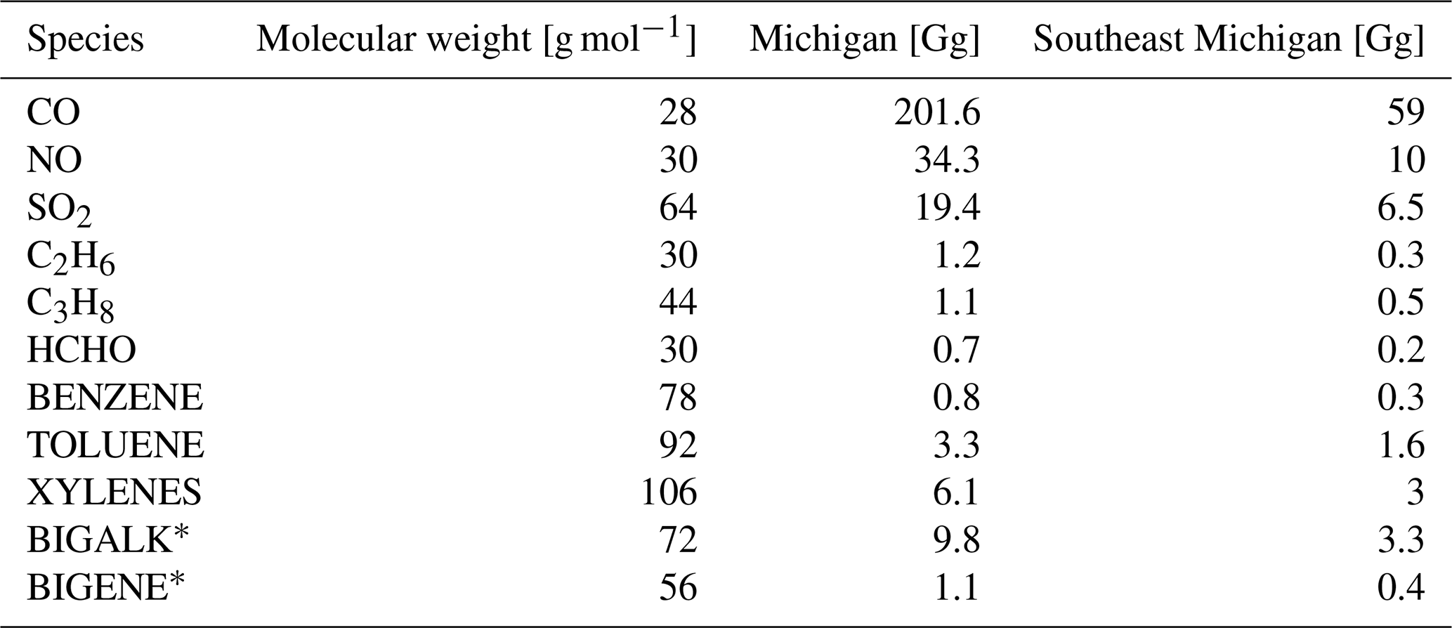
^* BIGALK represents lumped alkanes of C >3 (i.e., butanes, C₄H₁₀, and larger); BIGENE represents lumped alkenes of C >3 (i.e., butenes and larger) (Emmons et al., 2020).

2.1.4 Application of a diurnal cycle for anthropogenic nitric oxide emissions

O₃ has a strong diurnal variation throughout the day in the summertime, due to various processes such as precursor emissions (i.e., NO_x, VOCs), solar radiation, titration by NO_x, dry deposition, and vertical mixing within the planetary boundary layer (PBL) (Lin et al., 2008). O₃ reaches peak concentrations in the afternoon through photochemical reactions between its precursor species in the presence of solar radiation and then decreases in the early morning through dry deposition and NO_x titration processes (Lin et al., 2008). These processes also lead to strong diurnal cycles for NO_x, where peak surface concentrations are achieved in the early mornings and minimum concentrations in the afternoon. Although global models currently account for long-range transport and emission variations, these models usually focus on concentrations of pollutants in the daytime (Lin et al., 2008). Diurnal cycles for anthropogenic emissions are currently not considered in CESM2. Simulating the diurnal patterns of chemical species accurately is important for assessing the impact of these atmospheric processes at maintaining this cycle (Lin et al., 2008) and are crucial factors in the evaluation of model uncertainties such as estimating long-range transport impacts on local air quality and pollution mitigation efficiency.

To better assess the present biases of O₃ and NO_x concentrations in MUSICAv0, a diurnal cycle for anthropogenic NO emissions from CAMSv5.1 was implemented, which can strongly influence areas with high anthropogenic emissions. While emissions of other anthropogenic compounds, such as VOCs, do have diurnal variations, we have implemented only the diurnal variation for NO emissions in this work, due to its dominant role in controlling tropospheric O₃ and titration processes. This is based on the incorporation of the diurnal cycle presented in Jo et al. (2023). NO emissions in SEMI from power generation (ENE), residential (RES), and on- and off-road transportation (TNR and TRO, respectively) make up a significant amount of total NO emissions in the state of Michigan, at 30, 47, 18, and 23 %, respectively (see Table S1 in the Supplement). In order to incorporate diurnal variations for NO emissions, we used sector- and country-specific temporal profiles based on Crippa et al. (2020). The temporal profiles for each emission sector are available in the supplemental information (see Fig. S2). Although the hourly profiles were originally developed for EDGAR, they are used in this study because both EDGAR and CAMSv5.1 emission inventories use similar sector distributions. These hourly profiles are based on the downscaling of annual emissions to hourly datasets per grid cell (Crippa et al., 2020). The diurnal cycle for anthropogenic NO emissions was applied to the ne30x8 and the ne30x16 model runs, which will, hereafter, be referred to as ne30x8 DIUR and ne30x16 DIUR, respectively.

2.2 Observations

2.2.1 Michigan–Ontario Ozone Source Experiment

With the designation of SEMI as a non-attainment area for O₃, MOOSE sought to determine possible attainment strategies and characterize what is driving the elevated O₃ levels in the region using a combination of aircraft, mobile, and in situ measurements. The Michigan Department of Environment, Great Lakes, and Energy (EGLE) partnered with various scientific agencies, including the US Environmental Protection Agency (US EPA), the National Aeronautics and Space Administration (NASA), the Ontario Ministry of Environment, Conservation, and Parks (MECP), and Environment Climate Change Canada (ECCC), as well as various university partners, to carry out this campaign in two phases, held in the summers of 2021 (Phase I) and 2022 (Phase II), with each phase taking place for 6 weeks in May and June of the corresponding year. The work presented here is based on Phase I of the MOOSE field campaign. All measurement locations and tracks are shown in Fig. 2.

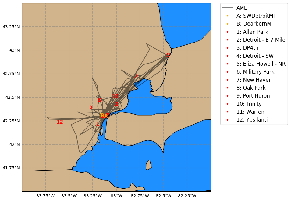
Figure 2 Locations of observations from Phase I (24 May to 30 June 2021) of the Michigan–Ontario Ozone Source Experiment (MOOSE) used in this study. The gray line shows the track of the Aerodyne Mobile Laboratory across Southeast Michigan. Stationary sites from the Michigan Department of Environment, Great Lakes, and Energy (MI EGLE) are shown as the red numbers (1–12), and the Pandora monitoring sites are shown as the yellow letters (A–B).

Aerodyne Mobile Laboratory (AML) measurements are available from 24 May to 30 June 2021 of Phase I. The AML drew in ambient air as it traveled throughout the SEMI region at a height of 2.8 m a.g. at 8 L per minute (Xiong et al., 2023). The Hemisphere GPS Compass (Model V100) was used to record the latitude and longitude of the AML. Consistent meteorological data of temperature, wind speed, and direction were measured by a sonic anemometer (2D R.M. Young Ultrasonic Anemometer, Model 85004). The AML deployed a variety of high-resolution, real-time instrumentation, including the Vocus Proton Transfer Reaction, Time-of-Flight, Mass Spectrometer (Vocus PTR-ToF-MS), Gas Chromatograph, Electron Impact, Time-of-Flight, Mass Spectrometer (GC-EI-ToF-MS), multiple Tunable Infrared Laser Direct Absorption Spectrometers (TILDAS), a LI-COR 6262 Non-Dispersive Infrared (NDIR), and a 254 nm 2BTech Model 205 Ozone Monitor. Table 2 further elaborates on the instrumentation, types of measurements, limits of detection, and resolution. The measurements reported along the AML tracks (see Fig. 2) allow for further elaboration on vehicular emissions and evaporated gases. Throughout the campaign, the AML sampled ambient air continuously and remained stationary in the nighttime at the Dearborn [42.3° N, 276.9° W] site.

Table 2 Detailed list of instrumentation on board the Aerodyne Mobile Laboratory during Phase I of the MOOSE field campaign.

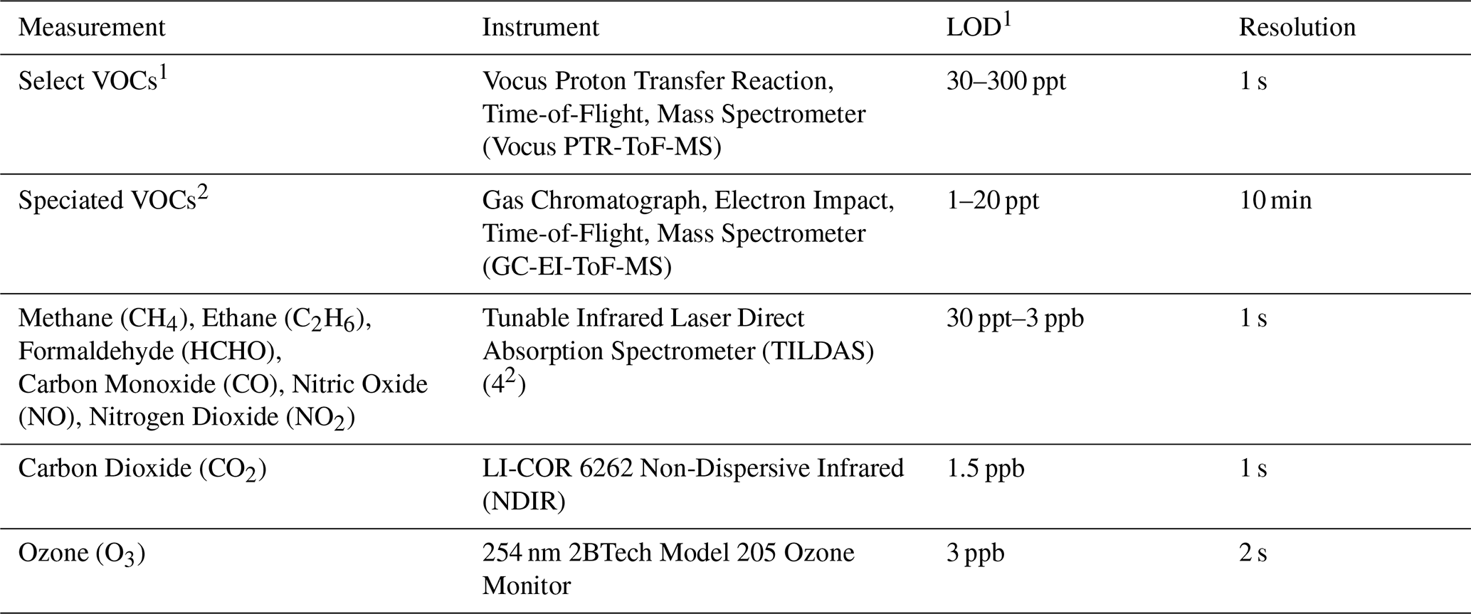
¹ Vocus PTR-ToF-MS measured for select VOCs, including acetaldehyde, methanethiol, acrolein, acetone, furan, cyclopentadiene, isoprene, sum of MEK + butanal, benzene, sum of ethyl acetate + pyretic acid, toluene, phenol, sum of C₈ aromatics, sum of C₉ aromatics, sum of C₁₀ aromatics, and sum of C₁₁ aromatics. ² GC-EI-ToF-MS measured speciated VOCs, including aromatics, halogens, oxygenates, and C₃–C₁₁ hydrocarbons.

Vertical columns of NO₂ and HCHO were measured using Pandora spectrometers (Herman et al., 2009) from the Pandonia Global Network (PGN) at two sites in SEMI – SWDetroitMI (Southwest Detroit, Michigan [42.30° N, 276.90° W]) and DearbornMI (Dearborn, Michigan [42.31° N, 276.85° W]) – available at https://data.pandonia-global-network.org/ (last access: 15 September 2025). Pandora uses spectroscopy to measure vertical column amounts of trace gases in the atmosphere (i.e., O₃, NO₂, HCHO), which absorb specific wavelengths of light from the sun in the ultraviolet-visible (UV/VIS) spectrum. Pandora has the ability to retrieve both direct-sun and all-sky radiance measurements. We use L2 direct-sun data products for the NO₂ and HCHO columns, which are reported to have higher precision and accuracy (Judd et al., 2019). This data product provides flags that indicate data quality and assure usability for scientific applications (Cede, 2021; Cede et al., 2023; Liu et al., 2024). Nine data quality flags are provided, where 0, 1, and 2 indicate assured high, medium, and low quality, respectively; data flags with a 1 in the tens position are preliminary and not quality assured, while a 2 in the tens position is an indication of data that are unusable for science. In this work, we applied the 0, 1, 10, and 11 data quality flags to obtain the vertical columns of NO₂ and HCHO per recommended use. To obtain the tropospheric NO₂ column from the direct-sun product, the climatological stratospheric component for NO₂, provided by PGN, was subtracted from the NO₂ total column. HCHO total columns were used because it is assumed that the majority of the HCHO column can be found in the well-mixed layer (Spinei et al., 2018). The HCHO distribution was observed within the 0–2 km altitude range and then gradually decreased with altitude, which is attributed to local surface emissions and photochemistry near the surface (Cheng et al., 2024).

In addition to Pandora, the NASA Langley Research Center Gulfstream III (G-III) aircraft was deployed during the campaign for 6 d between 5 and 24 June 2021 to retrieve the column density of NO₂ using the GEO-CAPE Airborne Simulator (GCAS) (Judd et al., 2020; Nowlan et al., 2016). GCAS is a UV/VIS spectrometer that provides NO₂ column measurements (below aircraft), operating in a push-broom motion, measuring backscattered light at wavelengths between 300 and 490 nm (Nowlan et al., 2018). The spatial resolution of these measurements is approximately 350 m across the track (30 pixels wide) and 650 m along the track. The sampling strategy for the G-III aircraft aims to simulate geostationary UV/VIS air quality mapping similarly to those expected from NASA TEMPO (Tropospheric Emissions: Monitoring of Pollution) (Chance et al., 2019) by measuring over an area of interest multiple times per day. Up to three maps per day were collected over the SEMI region during MOOSE flight days. For this study, we use NO₂ columns below the aircraft from the initial release (R0), applying cloud and glint flags.

2.2.2 Other observations used for model evaluation

Stationary measurements throughout SEMI were used to further evaluate the model simulations of NO. Real-time hourly measurements of O₃, NO₂, temperature, wind speed, and wind direction are available at various sites maintained by Michigan EGLE, as part of the Michigan Air Sampling Network (MASN). Measurements are collected by the state of Michigan using federal reference or equivalent monitoring methods approved by the US EPA. Data are made available at https://www.michigan.gov/egle/about/organization/air-quality/air-monitoring (last access: 15 September 2025). A detailed list of the sites and the observations obtained in SEMI can be seen in Table 3. In addition to the sites maintained by EGLE, during the MOOSE campaign, O₃ and NO₂ instrumentation was co-located with instruments already present at the Trinity-St. Mark's site in Detroit, Michigan, and the New Haven site in New Haven, Michigan.

Table 3 List of site information and observations obtained in Southeast Michigan through the Michigan Air Sampling Network (MASN) in the summer of 2021, where the numbers 1–12 are associated with Fig. 2.

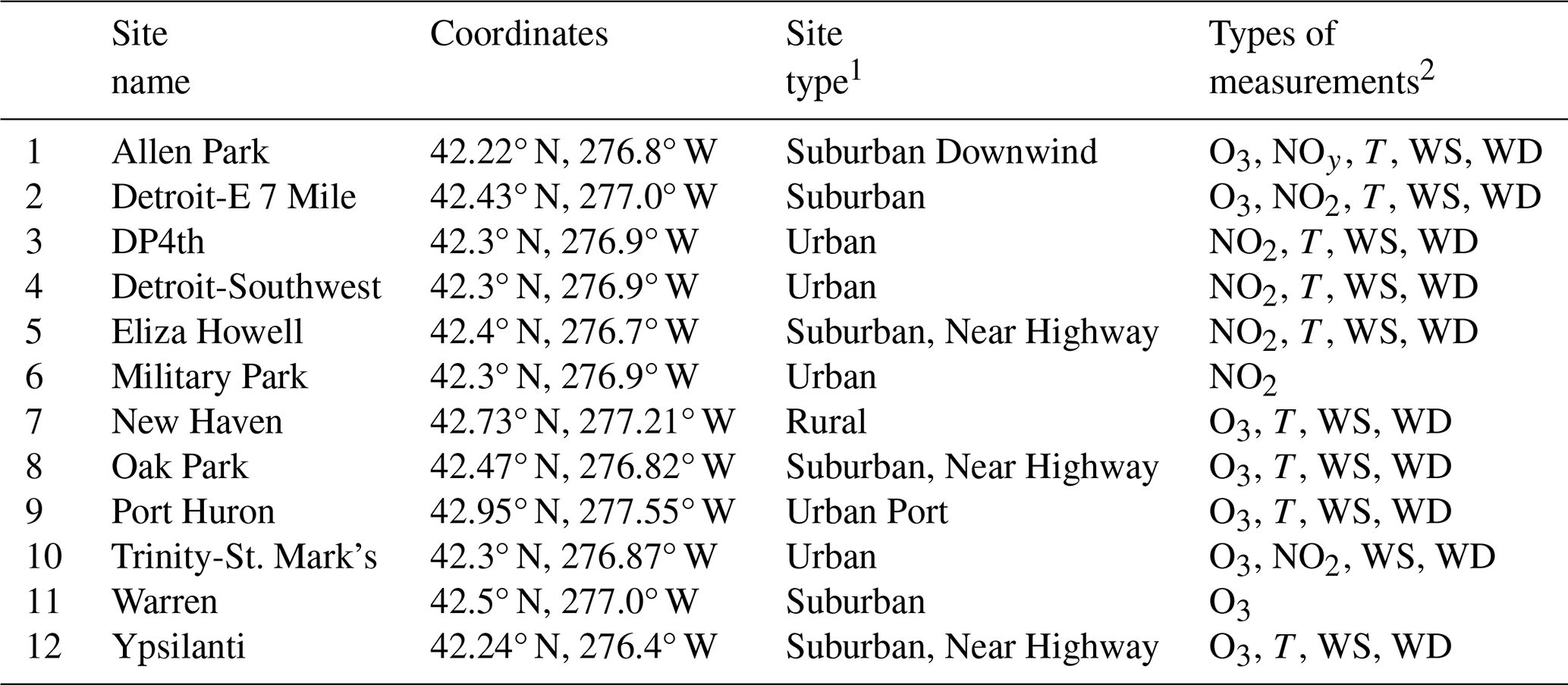
¹ Description of the types of measuring locations. ²O₃= Ozone; NO = Nitric Oxide; NO₂= Nitrogen Dioxide; NO_y= sum of NO_x and all other reactive nitrogen; T= temperature; WD = wind direction; WS = wind speed.

3 Results

In this section, we evaluate MUSICAv0 model results with observations from the MOOSE field campaign in May to June 2021. For evaluation, we compare the models with O₃ and NO₂ from MI EGLE stationary sites, a range of gas-phase species from the AML, NO₂ and HCHO columns from two Pandora spectrometers in SEMI, and NO₂ columns from GCAS. We evaluate the models using diverse datasets from MOOSE for a comprehensive analysis, as no single dataset has the ability to capture all aspects of atmospheric composition (e.g., emissions, chemistry, transport, meteorology). These different datasets can also help capture different aspects of a model such as near-surface chemistry (i.e., in situ measurements) and column burdens (i.e., aircraft-based remote sensing) to determine model skill, characterize model errors, improve model representation, and measure our confidence in the model results for reproducing reality.

For the comparison, we match the observed mixing ratios to the closest model grid point at each time. Modeled NO₂ and HCHO columns are calculated for the troposphere using the NO₂ and HCHO mixing ratios at each level of the model and multiplying them by the number density of air, which changes with altitude due to decreasing pressure, to get the number concentrations. Once the number concentrations are obtained, we multiply them by the layer thickness and integrate up to the average height of the column (i.e., for Pandora, the approximate height used was ∼ 3 km; for GCAS, the altitude of the aircraft was ∼ 12 km).

O₃ concentrations are highly associated with NO₂, where NO_x, in general, plays a critical role in the photochemical production and destruction of O₃ in the presence of sunlight. O₃ production in the troposphere is largely dependent on the availability of NO_x and VOCs and can give great insight into O₃ control. This dependency is classified into NO_x- and VOC-limited regimes. In a NO_x-limited regime, the rate of O₃ production relies on the abundance of NO_x and increases with NO_x concentrations but is not dependent on the concentrations of VOCs (Wang et al., 2019). In action, decreasing NO_x concentrations would lead to reductions in O₃ (Jacob, 1999). On the other hand, in a VOC-limited regime (or NO_x-saturated regime), the rate of O₃ production increases with VOC concentrations and is not dependent of NO_x (Wang et al., 2019); therefore, reducing the amount of VOCs would lead to reductions in O₃ (Jacob, 1999). The chemical relationship among O₃-NO_x-VOCs is critically important for defining mitigation strategies set to improve O₃ from region to region.

3.1 Meteorological consistencies

SEMI is a region that faces unique air quality challenges due to large industrial and automotive activity, dense population, and geographic factors. SEMI has a diverse terrain, ranging from highly urbanized areas, such as the city of Detroit, expansive agricultural lands in more remote areas, and forests surrounded by both inland and coastal lakes. The region consists of a relatively flat terrain, with a humid continental climate. Additionally, large air masses of humidity can be transported into the region from the Great Lakes (i.e., Lake Huron and Lake Erie) through the lake effect winds (Scott and Huff, 1996). A time series along the AML track of meteorological values – temperature, relative humidity, planetary boundary layer height, cloud total, wind speed, and wind direction – from the models (and observations for temperature and relative humidity) is shown in Fig. 3. During the campaign period in the summer of 2021, temperatures reached up to approximately 305 K, and relative humidity, to almost 100 %. The planetary boundary layer reached more than 2500 m on most days, while cloud total was relatively varied. Modeled wind speeds follow the trend for the campaign period quite well but are comparatively high compared to the observations, while wind directions perform generally well except on some specific days. The AML track covered a large part of the SEMI region, making its way through both very urban and rural areas. Meteorological parameters, such as temperature, are highly impacted by urbanization through the reductions in vegetated land cover and increases in energy consumption (Wang et al., 2021). Urbanization can lead to higher temperatures, thus increasing O₃ production. In the simulations presented here, meteorological parameters (i.e., temperature and horizontal winds) are nudged towards reanalysis data to obtain a more realistic depiction of reality in the coarser-resolution regions, leaving the regional refinement area to freely run, as the resolution of the refined area is finer than the resolution of the reanalysis dataset that is being used. Regional refinement grids, with high horizontal resolution, are capable of resolving areas with large geographical differences (Jo et al., 2023). Meteorological fields in these simulations are generally consistent, indicating that meteorology is performing similarly, even with the changes in horizontal resolution. Although temperature, relative humidity, and planetary boundary layer height remain consistent among all the simulations, cloud total varies between the simulations, which can significantly impact photochemical production.

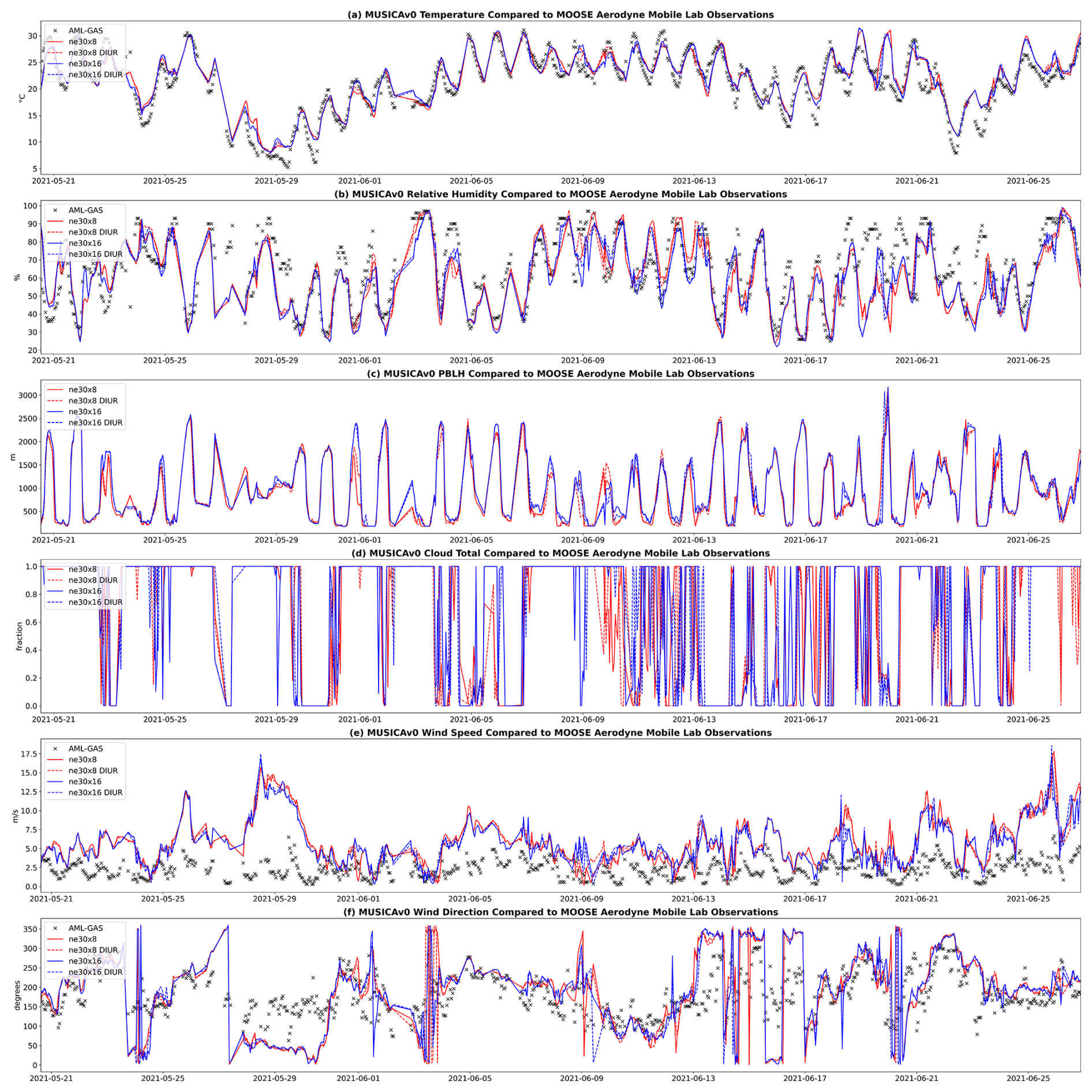
Figure 3 Time series of (a) temperature, (b) relative humidity, (c) planetary boundary layer height, (d) cloud total, (e) wind speed, and (f) wind direction along the Aerodyne Mobile Laboratory (AML) track. Measurements of temperature, relative humidity, wind speed, and wind direction are available and displayed as black x's. The model results are shown in red (ne30x8) and blue (ne30x16), corresponding to the horizontal resolutions. The dashed lines represent model simulation results when adding the diurnal cycle for nitric oxide anthropogenic emissions, color-coded to their respective horizontal resolution.

3.2 Evaluation with stationary sites

In this section, we evaluate the model results from four simulations during Phase I of the MOOSE field campaign (24 May to 30 June 2021) with real-time hourly measurements of O₃ and NO₂ from available stationary sites in SEMI, maintained by Michigan EGLE, as part of MASN. The stationary sites are located in an environment with mixed urban, suburban, and rural plumes (Fig. 2; descriptions in Table 3). For NO₂, available measurements are primarily located in urban and suburban areas.

The evaluation of the four model simulations with stationary measurements for O₃ at seven locations in SEMI – Allen Park (Suburban Downwind), Detroit-E 7 Mile (Suburban), New Haven (Rural), Oak Park (Suburban, Near Highway), Port Huron (Urban Port), Warren (Suburban), and Ypsilanti (Suburban, Near Highway) – are shown in Fig. 4 as time series of their hourly averaged diurnal profiles during the MOOSE campaign. Table S2 lists the mean bias (MB), root-mean-squared error (RMSE), and Pearson correlation (CORR) for O₃ at the selected stationary sites. In general, the ne30x16 simulations without diurnal cycle implementation performed well compared to stationary observations, with overall mean biases of −0.85, −1.12, −0.52, and 2.46 ppb for the New Haven, Oak Park, Warren, and Ypsilanti sites, respectively. Adding the diurnal cycle for NO further improved mean biases at the New Haven, Oak Park, and Warren sites, with overall mean biases of −0.22, 0.02, and 0.47 ppb, respectively. During 09:00–11:00 EDT, all model simulations miss the mark at all sites when the slope increases in the morning, which coincides with higher modeled NO₂ concentrations (see Fig. 5). On the other hand, Fig. 4 shows that ne30x8, with and without diurnal cycle implementation, tends to overestimate O₃ concentrations during peak ozone times (12:00–18:00 EDT), with mean biases of up to 10 ppb. During this time frame, the changes from the addition of the diurnal cycle for NO are minimal, with the largest differences resulting from the changing horizontal resolution. Increasing horizontal resolution reduces O₃ concentrations, bringing them closer to the observational datasets. A larger difference in modeled O₃ compared to observations occurs during minimum O₃ times (03:00–09:00 EDT), where differences can exceed 12 ppb. During these times, O₃ concentrations tend to be underestimated at most sites, with the exception of New Haven and Ypsilanti, where O₃ concentrations from the models are higher than the observations. The application of the diurnal cycle for anthropogenic NO emissions in both horizontal resolutions showed overall improvements in O₃, likely as a result of better performance in NO₂, which is demonstrated in Fig. 5.

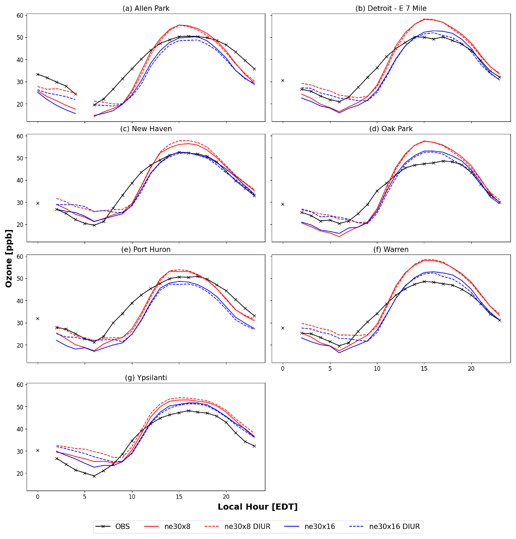
Figure 4 Model evaluation of hourly averaged diurnal profiles of ozone concentrations at the surface during the Michigan–Ontario Ozone Source Experiment (24 May to 30 June 2021) at seven stationary measurement sites in Southeast Michigan – (a) Allen Park [42.2° N, 276.8° W]; (b) Detroit – E 7 Mile [42.4° N, 277.0° W]; (c) New Haven [42.7° N, 277.2° W]; (d) Oak Park [42.5° N, 276.8° W]; (e) Port Huron [43.0° N, 277.6° W]; (f) Warren [42.5° N, 277.0° W]; and (g) Ypsilanti [42.2° N, 276.4° W]). The stationary measurements are shown in black, and the model results are shown in red (ne30x8) and blue (ne30x16), corresponding to the horizontal resolutions. The dashed lines represent model simulation results when adding the diurnal cycle for nitric oxide anthropogenic emissions, color-coded to their respective horizontal resolution. The gaps in the time series of the figures represent missing data at those locations.

Figure 5 shows the hourly averaged diurnal profile of NO₂ at six locations in SEMI – Detroit-E 7 Mile (Suburban), Detroit-SW (Urban), DP4th (Urban), Eliza Howell-NR (Suburban), Military Park (Urban), and Trinity-St. Mark's (Urban). Table S3 lists the statistical data for NO₂ concentrations at these stationary sites. NO₂ concentrations in the default simulations at the ne30x8 and ne30x16 horizontal resolutions had mean biases between 2 and 4 ppb. After implementing the diurnal cycle for NO anthropogenic emissions, the mean biases shifted between 0 and 3 ppb (dashed line in Fig. 5), with the exception of the Eliza Howell-NR site, which was greatly underestimated in all model simulations, with overall absolute mean biases of up to 11 ppb. This large underestimation at the Eliza Howell-NR site is highly attributable to the near-road transportation emissions that were not captured by the model. In general, although there are differences in NO₂ concentrations from the changing resolutions, where urban sites showed an increase in concentrations when going to finer resolution, the large differences came from the addition of the NO diurnal cycle. During peak times, the default configurations at each resolution showed higher concentrations of NO₂. Adding the diurnal cycle lowered these concentrations, bringing them closer to the observations. The application of the diurnal cycle for NO lowers NO emissions in the nighttime, bringing concentrations closer to the observed values during those times, which could in turn affect O₃ concentrations.

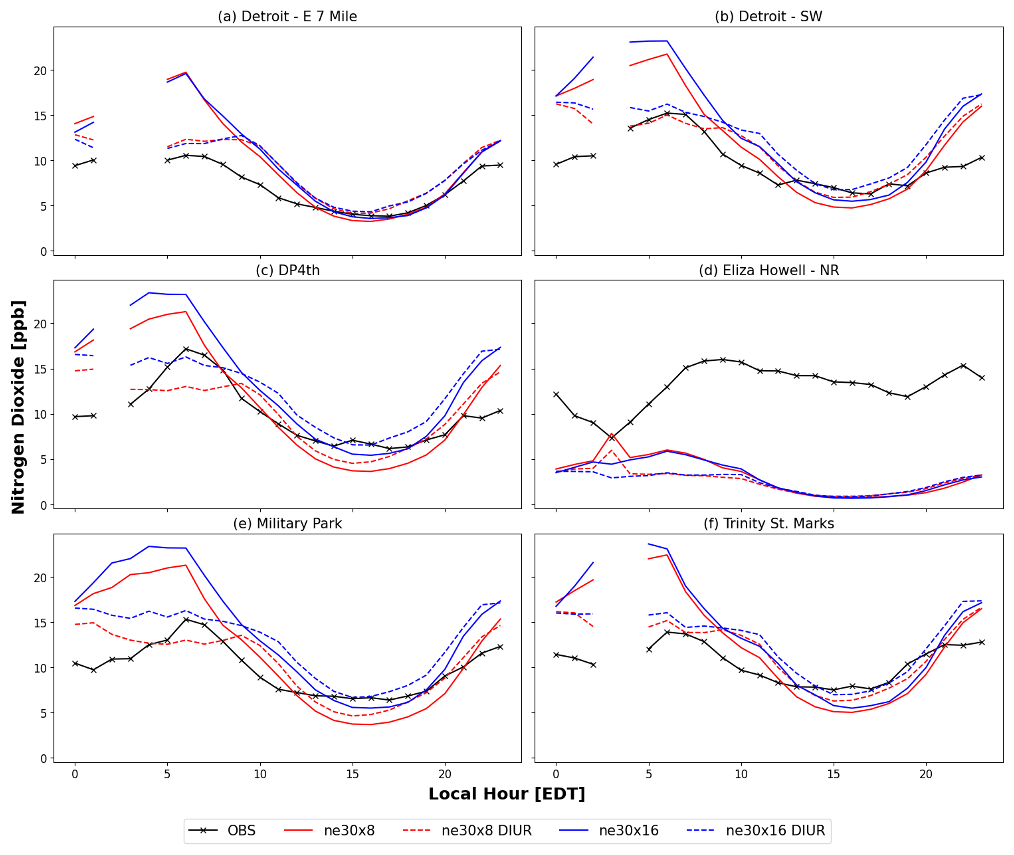
Figure 5 Same as Fig. 4 but for NO₂ with select stationary measurements from (a) Detroit – E 7 Mile [42.4° N, 277.0° W]; (b) Detroit – SW [42.3° N, 276.9° W]; (c) DP4th [42.3° N, 276.9° W]; (d) Eliza Howell – NR [42.4° N, 276.7° W]; (e) Military Park [42.3° N, 276.9° W]; and (f) Trinity-St. Mark's [42.3° N, 276.9° W].

3.3 Evaluation with Aerodyne Mobile Laboratory

Here, we evaluate the four MUSICAv0 simulations against mobile observations obtained from AML during Phase I of the MOOSE field campaign using a Taylor diagram (Taylor, 2001). Taylor diagrams allow us to summarize how closely model simulations match with observations using a combination of the Pearson correlation, the centered normalized root-mean-square difference, and the normalized standard deviation. A quality assurance flag was applied to the AML dataset, where we filtered the data to exclude measurements affected by traffic or self-sampling. Figure 6 compares gas-phase species from the AML to four MUSICAv0 simulations, where the observations from AML are used as the reference (black star). Detailed statistics for all available gas-phase species and meteorological parameters can be found in Tables S4 and S5, respectively. The further the simulation results are from this reference point, the poorer the model performance. Of the chemical species presented in Fig. 6, differences based on the different regional refinement grids were significant for some species (i.e., HCHO, isoprene), while for others, the differences were more dependent on the application of the diurnal cycle (i.e., O₃). These differences are discussed in Sect. 4. For surface O₃ concentrations (Fig. 6a), applying a diurnal cycle for anthropogenic NO increased performance in both regional refinement grids, with little difference between the grid resolutions. In contrast, NO, NO₂, and NO_x (Fig. 6c, d, e) performance varied compared to the AML measurements, where NO concentrations at the surface performed similarly between all model configurations, with slight improvements when adding the diurnal cycle. The NO₂ and NO_x simulation, on the other hand, did see a larger impact with both grid resolution and diurnal cycle application, where the ne30x16 run performed best compared to the observations. The differences in grid resolution are seen more strongly than the inclusion of diurnal NO emissions for HCHO concentrations in Fig. 6b. Isoprene is the main precursor of HCHO at the surface and a stimulant of O₃ production (Wolfe et al., 2016). Figure 6k shows that isoprene is simulated better with the ne30x16 grids, which can be associated with the grid resolution. Grid resolution can have a more significant impact on isoprene because BVOCs are calculated online in the model, where spatial resolution can impact meteorological fields and affect BVOC calculations. Although temperatures are not greatly affected by grid resolution, as was seen in Fig. 3, cloud totals are different in the two resolutions , which can impact the amount of solar radiation reaching the surface. Clouds in the model can be impacted by several changes, such as changes in aerosols, which is out of the scope of this study, or changes in meteorology (e.g., winds). Yan et al. (2023) demonstrated that aerosols are able to impact precursor accumulation and photolysis (e.g., isoprene), where tropospheric chemical loss is enhanced due to photolysis and NO_x accumulation. Cheng et al. (2022) also found that changing clouds in chemical transport models can impact photochemical reaction rates and BVOCs. Future work on evaluating model grid resolution and diurnal cycle impacts on O₃ formation should look more closely into aerosol–cloud interactions and how they impact photochemical production in SEMI. Additionally, Fig. 6l shows α-pinene, which performs similarly across all simulations, regardless of the resolution and application of a diurnal cycle for anthropogenic NO emissions. Unlike isoprene, where changes from the BVOC calculations in MEGANv2.1 were more pronounced, α-pinene was generally unchanged across all of the simulations. Figure 6f–h includes ethane (C₂H₆), propane (C₃H₈), and propene (C₃H₆), respectively, which are important hydrocarbon precursors of O₃ in areas with many anthropogenic sources. C₂H₆ is primarily emitted via extraction and processing of fossil fuels, while C₃H₈ and C₃H₆ are emitted mainly through petroleum gas industries (Emmons et al., 2020). All MUSICAv0 simulations generally perform similarly when compared with the observations of these species, with relatively low correlation. The models underestimate C₂H₆, C₃H₈, and C₃H₆, which is an indication of missing emission sources. Benzene and toluene are also important O₃ precursors, emitted from anthropogenic sources (Fang et al., 2016) such as solvent usage, incomplete combustion, industrial coatings, and the petroleum industry. Both benzene and toluene (Fig. 6i, j) are underestimated in the models, again likely as a result of missing emission sources, with a small improvement in benzene as a result of grid resolution. Percent differences are shown in Fig. S1 to further demonstrate the consistent misrepresentation of C₂H₆, C₃H₈, C₃H₆, benzene, toluene, and α-pinene in MUSICAv0 regardless of model modifications. As chemistry–climate models move to finer resolutions (< 10 km), local emission sources will need to be represented more accurately for proper use in fine-scale scientific applications. Additionally, future work should focus on evaluating simulations with the application of diurnal cycles to all anthropogenic emission sources, as they can vary greatly during the day from sector to sector.

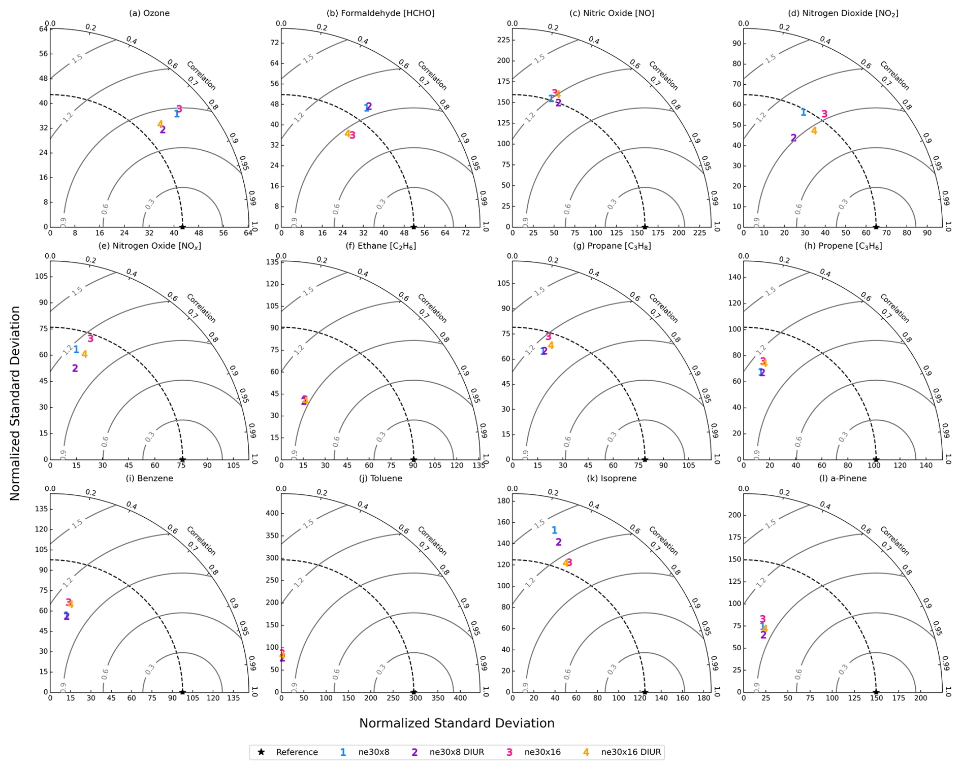
Figure 6 Taylor diagrams comparing gas-phase species from the Aerodyne Mobile Lab (AML) to MUSICAv0 simulations during the Michigan–Ontario Ozone Source Experiment (24 May to 30 June 2021). The different simulations are represented by numbers, where each color represents a different model configuration. The reference point (star symbol) represents the observations from the AML. The correlation corresponds to the angular axis, and the normalized root-mean-squared error, to the radial axis.

3.4 Evaluation with Pandora spectrometers

We compare the NO₂ and HCHO tropospheric columns from two Pandora spectrometers to the four MUSICAv0 simulations. Both Pandora monitoring sites (SWDetroitMI and DearbornMI) were located in an industrial and high-traffic setting, providing continuous observations in urban conditions and complementing the other observations. Figures 7 and 8 show hourly binned box-and-whisker plots of NO₂ and HCHO columns between 9 and 30 June 2021 for the SWDetroitMI and DearbornMI sites in SEMI, respectively, compared to the model simulations. These locations are presented in Fig. 2. All of the model simulations performed well when compared to the NO₂ columns from Pandora. Overall, observed means were lower than modeled means, indicating an overestimation in the modeled NO₂ column. During peak NO₂ time frames (07:00–11:00 EDT) at the SWDetroitMI site, modeled NO₂ columns saw improvements resulting from the application of the diurnal cycle for anthropogenic NO. In the afternoon, the NO₂ columns in the models gradually increased, going from coarser to finer resolution and with the added diurnal cycle. Although the difference in grid resolution plays a role in the simulation of NO₂ columns, the differences were not as significant in the later part of the day. The modeled and observed NO₂ columns were better represented when both higher resolution and the application of the diurnal cycle for anthropogenic NO were included, with correlations of 0.28 and 0.31 at the SWDetroitMI site and 0.61 and 0.58 at the DearbornMI site. Consequently, the HCHO columns also performed well at the SWDetroitMI and DearbornMI sites during the early morning (07:00–09:00 EDT). On the other hand, after 10:00 EDT, the models began underestimating the HCHO columns, with differences of nearly a factor of 2. The locations of the Pandora spectrometers are in highly industrialized, urban areas. The large model bias in the HCHO columns could be an indication of missing emission sources in the area. In addition, as was mentioned in Sect. 3.3, cloud formation also changes in the simulations, which could impact BVOC emissions, such as isoprene (main precursor of HCHO) and photolysis rates, and ultimately impact HCHO columns. A combination of grid resolution and the diurnal cycle is largely responsible for increased HCHO columns, bringing the model closer to the measurements, with correlations for the ne30x8 and ne30x16 model runs of 0.30 and 0.22 at the SWDetroitMI site and 0.38 and 0.30 at the DearbornMI site, respectively. Detailed statistics for the NO₂ and HCHO tropospheric columns from Pandora at the SWDetroitMI and Dearborn MI sites, along with the four model simulations, can be found in Tables S6 and S7, respectively.

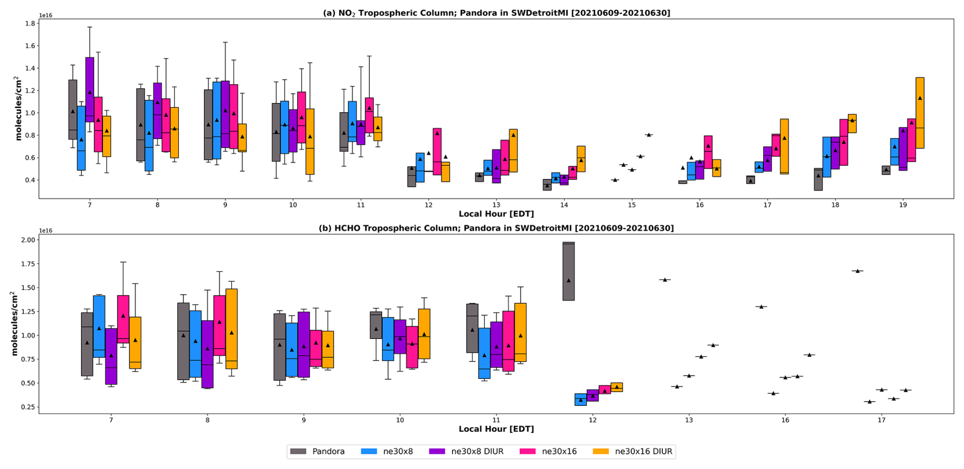
Figure 7 Hourly binned box-and-whisker plots showing Pandora NO₂ (a) and HCHO (b) tropospheric columns (in gray) and modeled tropospheric columns at the SWDetroitMI [42.30° N, 276.90° W] site in Southeast Michigan. The tropospheric columns from the model simulations were calculated up to approximately 3.3 km (10 model levels), as the average height obtained from the Pandora spectrometers was about 3 km. The box-and-whisker plots show the 10th, 25th, 50th, 75th, and 90th percentiles, where the triangles are representative of the means.

Figure 8 Same as Fig. 7 but for the Pandora spectrometer located at the DearbornMI [42.31° N, 276.85° W] site in Southeast Michigan.

3.5 Evaluation with GCAS

In this section, we qualitatively evaluate modeled NO₂ tropospheric columns against observed NO₂ tropospheric columns from the GCAS instrument on board the NASA G-III research aircraft. While GCAS measures the column amount of NO₂ below the aircraft, the surface concentrations generally dominate the column in the lowest part of the atmosphere. Figures 9–11 show the comparison of the modeled NO₂ columns from the four simulations discussed in this paper with the observed GCAS NO₂ columns in SEMI on 11 June 2021 for the three flights of the day. The details for each flight day can be found in Table S8, and day-to-day variabilities for the remaining days can be found in the Supplement, Figs. S3–S15. The day of Friday, 11 June 2021 exhibited a moderate air quality index (AQI) with temperatures between 24 and 30 °C and calm wind speeds at 2–5 m s⁻¹. The overall wind direction during the flight times was from the east in SEMI. In the area, plumes of NO₂ can be observed from source locations such as power plant emissions in Monroe, Michigan, mobile and industrial emissions in Detroit, Michigan, additional power generation emissions in East China, Michigan, and emissions from Sarnia's “Chemical Valley” in Ontario, Canada, which includes various petrochemical facilities.

Figures 9–11 demonstrate the hourly variabilities of NO₂ columns in the model and observations for 11 June 2021. Three rasters were sampled on this day, between mid-morning and mid-afternoon. In general, the NO₂ tropospheric columns from GCAS were higher in the morning than they were in the afternoon. All four model simulations followed a similar trend (in Figs. 9–11 and in the Supplement), where the NO₂ columns were higher in the mornings compared to the afternoon. Although the NO₂ source regions are identifiable in all of the model simulations, the finer grid mesh better resolves the source regions and makes NO₂ plumes more visible in all of the time frames. The model simulations at the ne30x16 resolution (Figs. 9–11b, 9–11e) show good agreement with the observed wind direction blowing from the northeast direction pushing NO₂ in the western direction (noted in Table S8). In general, the magnitude differences between the coarse and fine grids and the application of the diurnal cycle for anthropogenic NO did not have a large impact on the NO₂ columns between simulations. What can be noted is that the ne30x16 horizontal resolution showed more pronounced pollution plumes from source regions and more defined NO₂ tropospheric columns. The directions of the pollution plumes are supported by plots of temperature and wind vectors in Figs. S16–S31 in the SI for each of the flight days. Even with a resolution of $\mathrm{1}/\mathrm{16}$° (ne30x16), some point sources captured by GCAS are not captured by the model because it is still relatively coarse for urban applications. With the future release of MUSICAv1, which uses the non-hydrostatic dynamical core MPAS (Model for Prediction Across Scales; on an unstructured grid mesh based on centroidal Voronoi tessellations, Du et al., 1999), allowing for regional refinement below 5 km, estimates of emissions at finer scales over regions of interest are necessary. Tropospheric NO₂ columns from satellites (e.g., TROPOMI, OMI) have been used to estimate NO_x emissions in localized environments (Goldberg et al., 2024; Martínez-Alonso et al. 2023; Dix et al., 2022; Beirle et al., 2019; Liu et al., 2016a). For example, Martínez-Alonso et al. (2023) used TROPOMI NO₂ columns to derive emissions from mining and industrial activities in the Democratic Republic of Congo and Zambia. In addition, Goldberg et al. (2024) used a combination of aircraft remote sensing (i.e., GCAS), source apportionment models, and regression models to investigate NO₂ emissions from individual sources in Houston, Texas. Future work should take into consideration the use of the GCAS observations to develop emission inventories for use in multi-scale model simulations of Michigan.

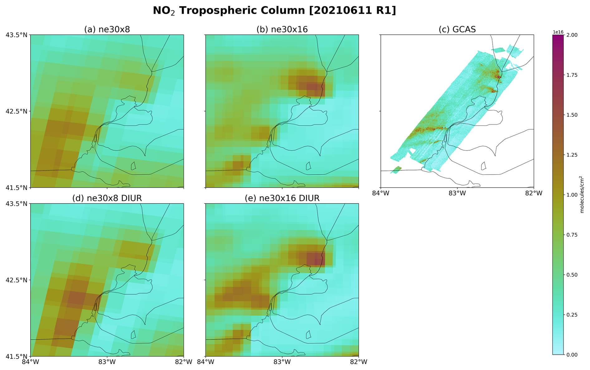
Figure 9 Modeled and observed NO₂ tropospheric columns over Southeast Michigan on 11 June 2021. The GCAS instrument flew over the Southeast Michigan region between 10:10 and 11:45 EDT, so the modeled NO₂ tropospheric columns were calculated using the 11:00 EDT time frame. Figure 9a, b, d, and e represent modeled NO₂ tropospheric columns calculated to about 12 km in altitude, which was the average flight altitude of the NASA Gulfstream-III aircraft. Figure 9c shows the observed NO₂ tropospheric column from the GCAS instrument during the morning time.

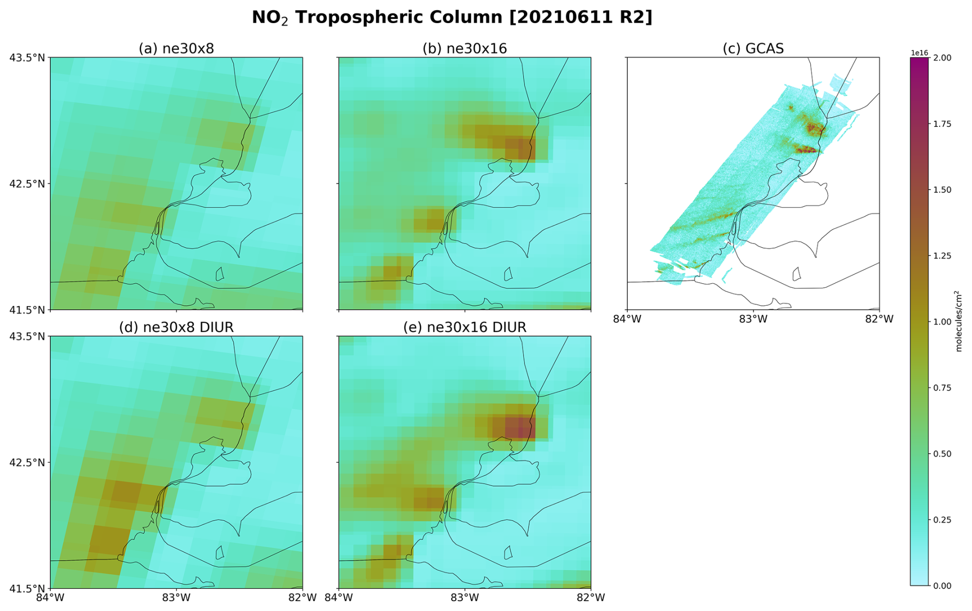
Figure 10 Same as Fig. 9, but the GCAS instrument flew over Southeast Michigan from 11:45 to 13:16 EDT, and the modeled NO₂ tropospheric columns were calculated during the 12:00 EDT time frame.

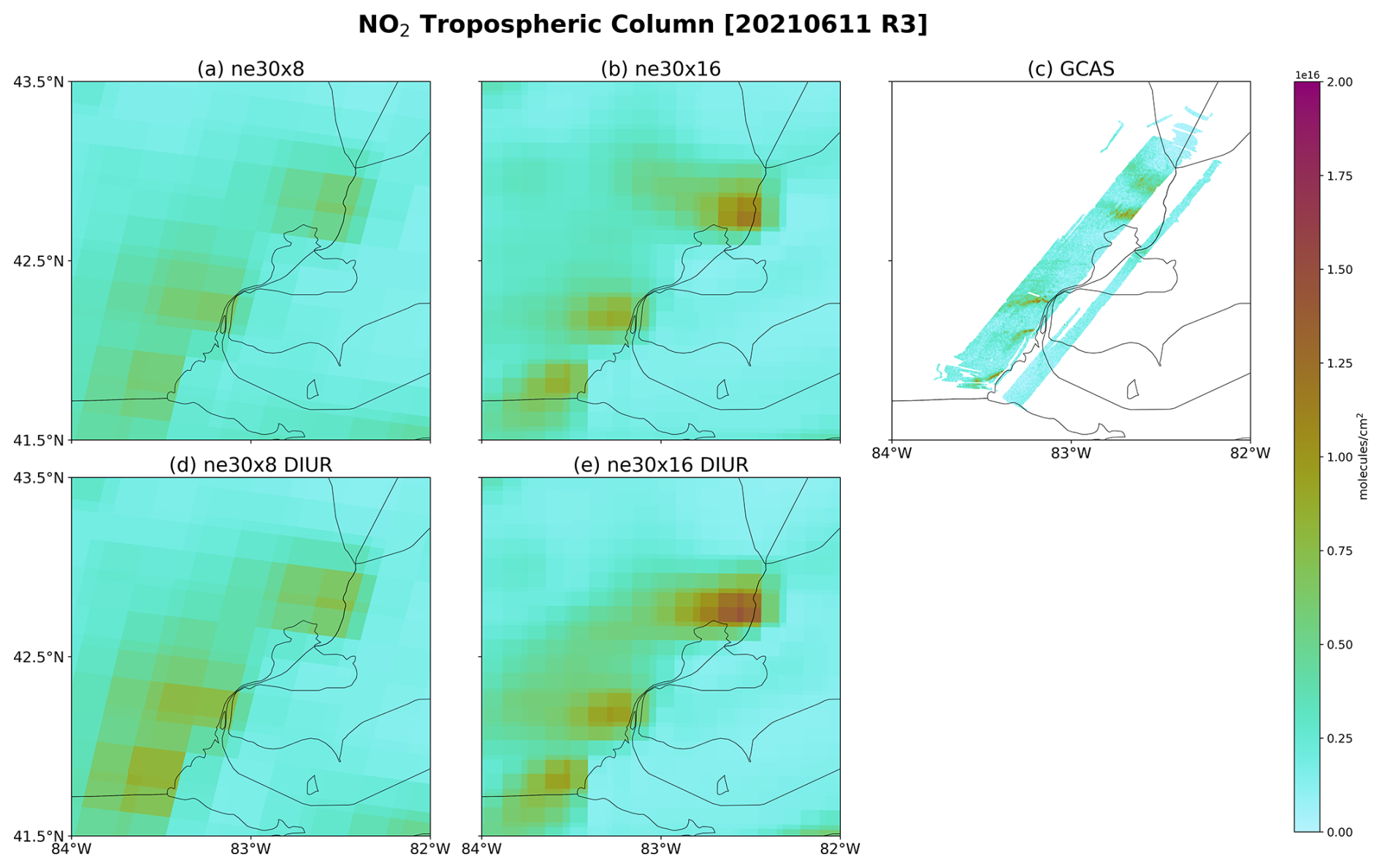
Figure 11 Same as Fig. 9, but the GCAS instrument flew over Southeast Michigan from 13:16 and 14:00 EDT, and the modeled NO₂ tropospheric columns were calculated during the 13:00 EDT time frame.

Section 3 evaluated the model simulations against four different types of observations obtained during MOOSE 2021. Taken together, the model evaluation shows that (i) refining the horizontal grid resolution in the model is the dominant factor leading to reductions in bias for peak O₃ concentrations, enhances NO₂ source region plumes, and better separates the contrast between urban and suburban locations, such as Allen Park and Trinity-St. Mark's; (ii) the diurnal cycle for anthropogenic NO emissions corrects the early morning biases in NO₂ and slightly impacts O₃, while having small impacts on peak O₃ values; and (iii) the high biases in VOCs point to deficiencies in the emission inventory rather than grid resolution and temporal allocation. These findings motivate the more in-depth analysis described in Sect. 4, where we discuss resolution- and diurnal emission-driven changes governing O₃ production and loss across SEMI.

4 Discussion: impacts of grid resolution and diurnally varying emissions

The previous section (Sect. 3) evaluated four MUSICAv0 simulations using two different regional refinement grids (ne30x8, ne30x16) and the addition of a diurnal cycle for anthropogenic NO emissions (ne30x8 DIUR, ne30x16 DIUR) against observations from Phase I of the MOOSE field campaign. Building on the evaluation in Sect. 3, this section discusses the differences resulting from changes in horizontal grid resolution and the application of the diurnal cycle for anthropogenic NO. We analyze how site-specific behaviors are driven by the model changes and how those behaviors drive O₃ formation. First, the spatial distributions in the two resolutions are compared (Figs. 12–14), and then the diurnal cycles in different environments are compared (Figs. 15–18).

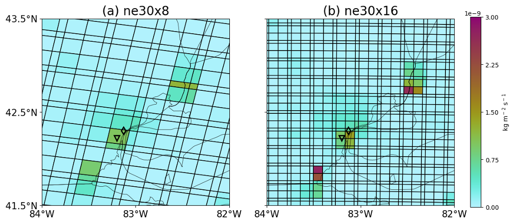
Figure 12 Nitric oxide (NO) emission distribution averaged for June and July 2021 over Southeast Michigan on corresponding regional refinement grids. Two SEMI sites – Allen Park (triangle) and Trinity-St. Mark's (diamond) – are shown relative to their grid box locations.

Figure 12 shows emissions of NO across the SEMI region and the different grid boxes pertaining to the (a) ne30x8 and (b) ne30x16 horizontal resolutions. The Allen Park and Trinity-St. Mark's ground sites (black triangle and diamond, respectively) are also shown relative to their grid box locations and the distribution of NO emissions. This figure shows that in the coarse resolution (Fig. 12a), the two sites (a suburban and an urban site) are represented by the same grid box, whereas in the finer, ne30x16 resolution (Fig. 12b), they are present in distinct grid boxes. Although the total emissions for a region are the same, emission fluxes can become more resolved when moving to a finer grid resolution (Jo et al., 2023), which will ultimately impact model simulation evaluation as the horizontal resolution becomes finer and finer.

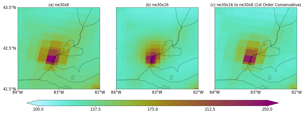
Figure 13 Modeled carbon monoxide (CO) concentrations at the surface for June 2021, where (a) is the ne30x8 horizontal resolution, (b) is the ne30x16 horizontal resolution, and (c) is the ne30x16 model output regridded to the coarser ne30x8 horizontal resolution using the first-order conservative method.

To quantitatively assess the impact of the finer resolution on the simulation of ozone and its precursors, the ne30x16 (7 km) results have been conservatively regridded to the ne30x8 grid. These regridded results illustrate the impact model resolution can have on atmospheric chemistry, depending on the compound. Figure 13 shows the modeled monthly averaged carbon monoxide (CO) concentrations at the surface for June 2021 for the ne30x8 (Fig. 13a), ne30x16 (Fig. 13b), and conservatively regridded model output from the ne30x16 simulations to the ne30x8 horizontal resolutions (Fig. 13c), respectively. CO is mainly emitted through incomplete combustion processes and has a generally long lifetime, lasting from week to months, allowing it to be transported over long distances (Gaubert et al., 2016). These characteristics make CO relatively chemically inactive. Because of this, there are minimal chemistry effects, where the majority of impacts on CO will result from the grid resolution. Fine-scale features of CO are better captured in the ne30x16 horizontal resolution simulations, as CO concentrations are more resolved over urban regions, as can be seen in Fig. 13b. Figure 13c shows the modeled CO concentrations, conservatively regridded from the ne30x16 horizontal resolution to the ne30x8 horizontal resolution. Using this regridding method to go from the finer to the coarser resolution did not reproduce the same results seen from running the ne30x8 simulation (Fig. 13a). When the model is run at $\mathrm{1}/\mathrm{16}$° horizontal resolution, localized features (e.g., pollution plumes, sharp emission gradients) are better resolved, and land use is better represented. Figure 13a–c have mean CO concentrations over SEMI of 141.7, 131.1, and 132.1 ppb, respectively.

On the other hand, O₃ is highly chemically active. Figure 14 shows modeled monthly averaged O₃ concentrations at the surface for June 2021 for ne30x8 (Fig. 14a) and ne30x16 (Fig. 14b), as well as the conservatively regridded model output from the ne30x16 simulations to the ne30x8 horizontal resolutions (Fig. 14c), respectively. Similarly to what Jo et al. (2023) found over South Korea, there is a decrease in O₃ concentrations over urban areas in SEMI as a result of NO_x titration. This reduction in O₃ is more prominent with the finer horizontal model grid resolution, which leads to differences in the monthly mean surface O₃ concentrations in coarse (40.1 ppb) and fine (38.0 ppb) horizontal resolutions over SEMI. When regridding O₃ concentrations from the finer to the coarser horizontal resolution, the NO_x titration is visible over the urban areas in SEMI, similarly to the ne30x16 simulation, but it is stronger when compared to the ne30x8 simulation.

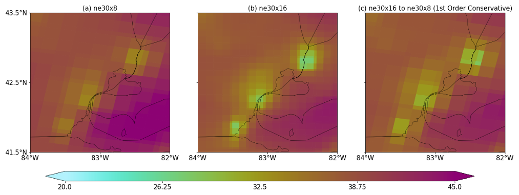
Figure 14 Same as Fig. 13 but for modeled O₃ concentrations at the surface.

Figure 15 shows the diurnal variation for O₃, NO, and NO₂ concentrations, NO emission flux, and the planetary boundary layer height from the four simulations presented in this study for three sites – a suburban downwind site (Allen Park), an urban site (Trinity-St. Mark's), and a rural site (New Haven). The Allen Park and Trinity-St. Mark's sites are located within the same grid box in the ne30x8 simulations, while in the ne30x16 simulations, they are not. Figure 15a–c show that horizontal resolution had the most impact on O₃ concentrations at all sites during peak times (12:00–18:00 EDT), with differences between simulations of up to ∼ 5 ppb. This difference results in an improvement for the ne30x16 simulations based on the findings in Fig. 4, where peak O₃ performed best in the finer-resolution simulations when compared to the surface sites. The addition of a diurnal cycle for anthropogenic NO did not have a significant impact on O₃ concentrations during these peak times but saw larger differences during the 05:00–11:00 EDT time frame, likely as a result of lower NO (Fig. 15d–f) and NO₂ (Fig. 15g–i) concentrations and associated NO_x titration in the model simulations. It is important that we acknowledge the differences caused in NO and NO₂ at the Allen Park and Trinity-St. Mark's sites due to the grid resolution. As was mentioned before, Allen Park and Trinity-St. Mark's are located within the same grid box in the coarser resolution. When using the ne30x16 horizontal resolution, higher concentrations for NO and NO₂ can be seen at the Trinity-St. Mark's site than at the Allen Park site, which coincides with the high urbanization in that area. Although these differences are not greatly significant to O₃ concentrations, it is important that urban and non-urban areas are distinguished, as they can have higher emissions fluxes (Fig. 15j–l).

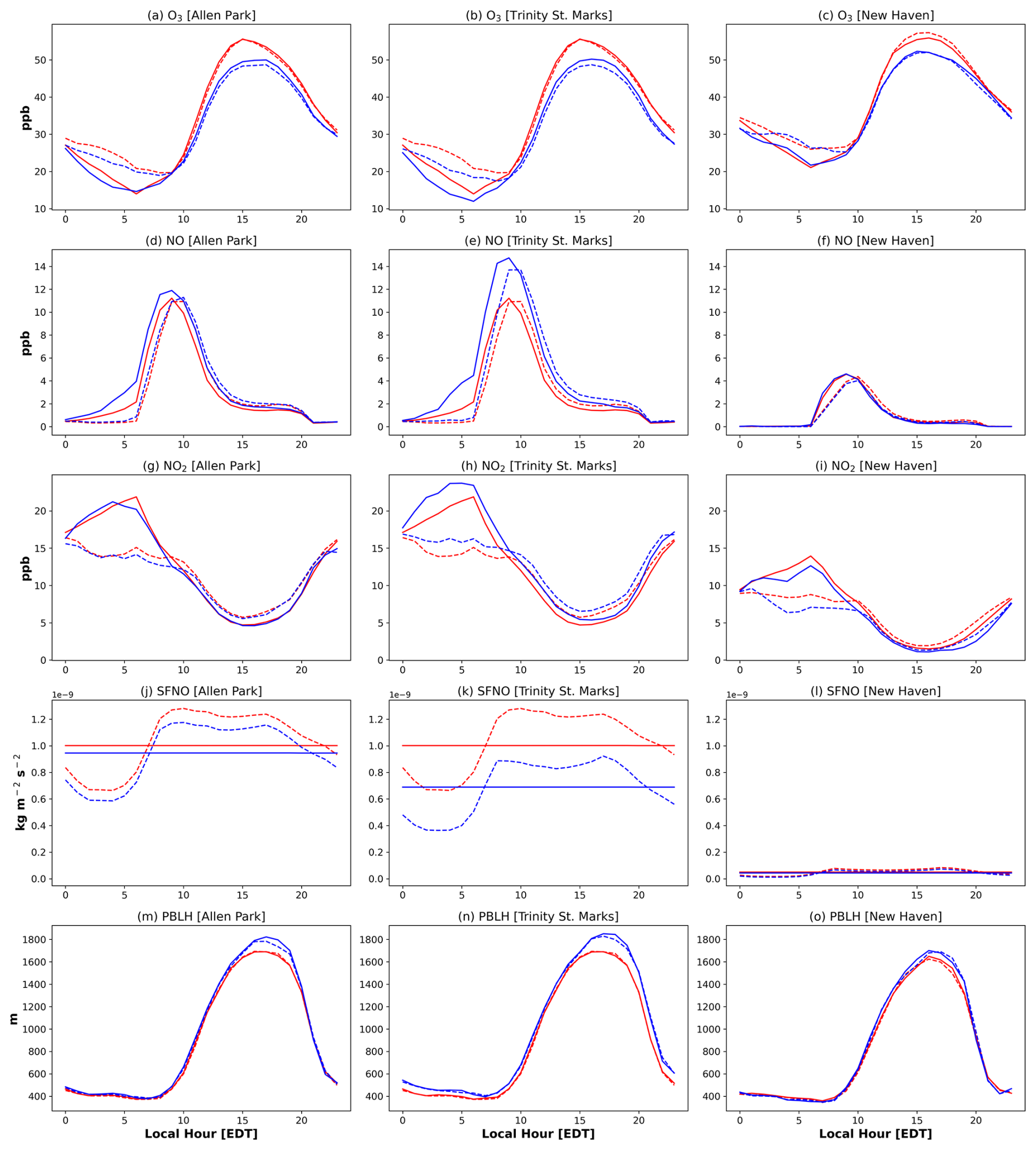
Figure 15 Diurnal cycle for O₃, NO, NO₂, NO surface flux (SFNO), and planetary boundary layer height (PBLH) for three sites in SEMI during Phase I of the MOOSE campaign [24 May to 30 June 2021] – a suburban downwind site (Allen Park), an urban site (Trinity-St. Mark's), and a rural site (New Haven). The ne30x8 simulations are represented by the red lines, whereas the ne30x16 simulations are represented by the blue lines. The application of the diurnal cycle to each simulation is represented by the dotted lines for each respective simulation.

On the other hand, a more rural site, like New Haven, has just as much O₃ as an urban site, even though NO emission fluxes are quite low. This is likely a result of the New Haven site being more representative of background concentrations driven by transport from upwind areas that include close proximity to a major highway and near Lake St. Clair. Hayden et al. (2011) found that along the Lake St. Clair shore, pollutants can be confined, leading to elevated pollutant concentrations and an increase in oxidizing capacity.

Biogenic VOC emissions can be heavily impacted by changes in model horizontal grid resolution, as they are based on meteorological parameters, such as temperature, because they are calculated online in the land model using the MEGANv2.1 algorithm (see Sect. 2.1.3). Figure 16 shows isoprene mixing ratios averaged over June and July 2021 from the ne30x8 (Fig. 16a) and ne30x16 (Fig. 16b) simulations, where the ne30x8 simulation shows about double the amount of isoprene compared to the ne30x16 simulation spread over a wider area. This can be explained by the higher isoprene emission fluxes in SEMI in the coarse resolution (Fig. 17a) compared to the finer resolution (Fig. 17b). These differences in isoprene emissions caused by the different horizontal resolutions directly impact isoprene concentrations in the models. These findings are directly supported by Fig. 3, where although temperatures between the simulations are not significantly different, there are changes in cloud totals and winds that could impact solar radiation and thus the isoprene emissions. The differences in temperature between the resolutions are also illustrated in the maps in Figs. S16–S31 in the Supplement.

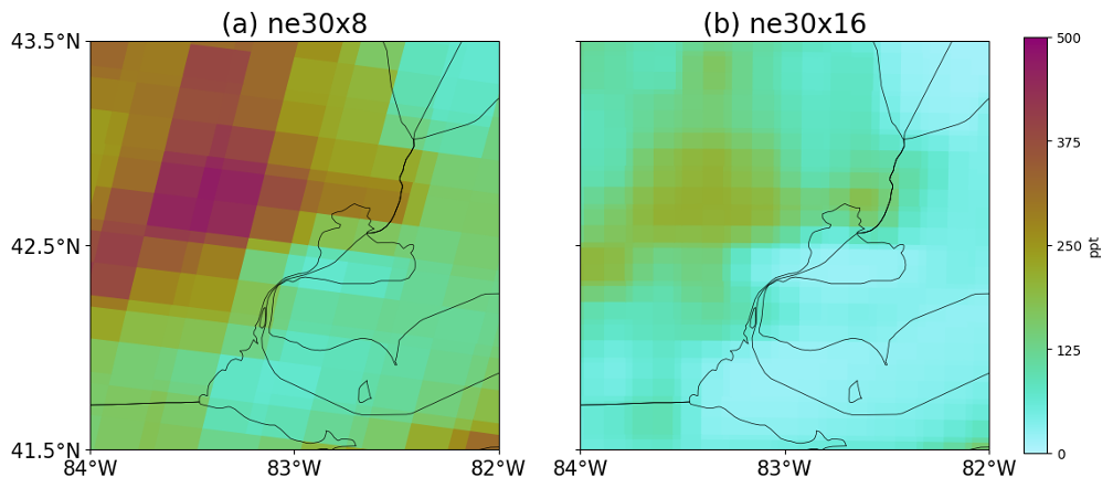
Figure 16 Modeled isoprene mixing ratios averaged for June and July 2021 over Southeast Michigan.

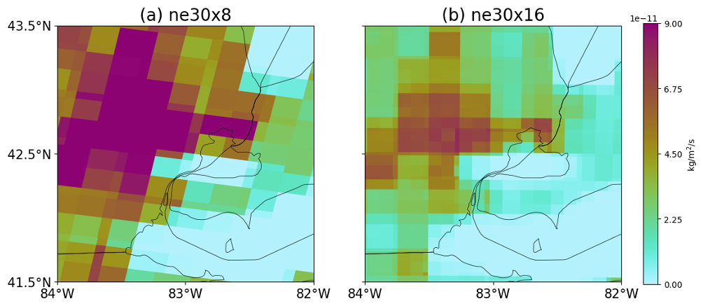
Figure 17 Isoprene emission flux averaged for June and July 2021 over Southeast Michigan.

Similarly to O₃ and NO₂, isoprene has a strong diurnal cycle that is driven by temperature and solar radiation. The diurnal cycles for isoprene, HCHO, and the hydroxyl radical (OH) are shown in Fig. 18 for the same three sites in Fig. 15. For the Allen Park and Trinity-St. Mark's sites, the isoprene mixing ratios (shown in Fig. 18a–c) were generally lower in both simulations, which coincides with suburban and urban landscapes that have relatively low densities of trees, while at the New Haven Site, the concentrations were about double compared to the other two sites, as it is a more rural region. For all of the sites, the isoprene concentrations were lower in the ne30x16 simulations compared to the ne30x8 simulations. In the ne30x8 simulations, the isoprene concentrations at the Allen Park and Trinity-St. Mark's sites are shown to be the same, but when using the ne30x16 resolution, isoprene is shown to be lower in the urban location compared to the suburban location. This indicates that finer resolution can help better characterize regions of interest and assist in the misclassification of emission sources, which coincides with the findings in Sect. 3. The lower isoprene concentrations also impact HCHO concentrations (shown in Fig. 18d–f), as HCHO is a product of isoprene oxidation. HCHO is lower in the ne30x16 simulations, which coincides with the lower isoprene concentrations. OH concentrations (shown in Fig. 18g–i) are generally consistent in all simulations, with very minimal changes after applying the diurnal cycle for anthropogenic NO. Because SEMI is in a more VOC-limited regime (Xiong et al., 2023), OH concentrations are less sensitive to changes in VOCs and more prone to changes resulting from the changing NO_x levels due to titration of O₃ (de Gouw et al., 2019). HCHO is NO_x sensitive, meaning that more HCHO is produced in the presence of higher NO_x concentrations (Schwantes et al., 2022). HCHO was not heavily changed by the application of the diurnal cycle for anthropogenic NO emissions, indicating that the main driver for changes in HCHO is grid resolution. In general, isoprene and HCHO decrease with increased resolution, while OH remains relatively constant between model simulations.

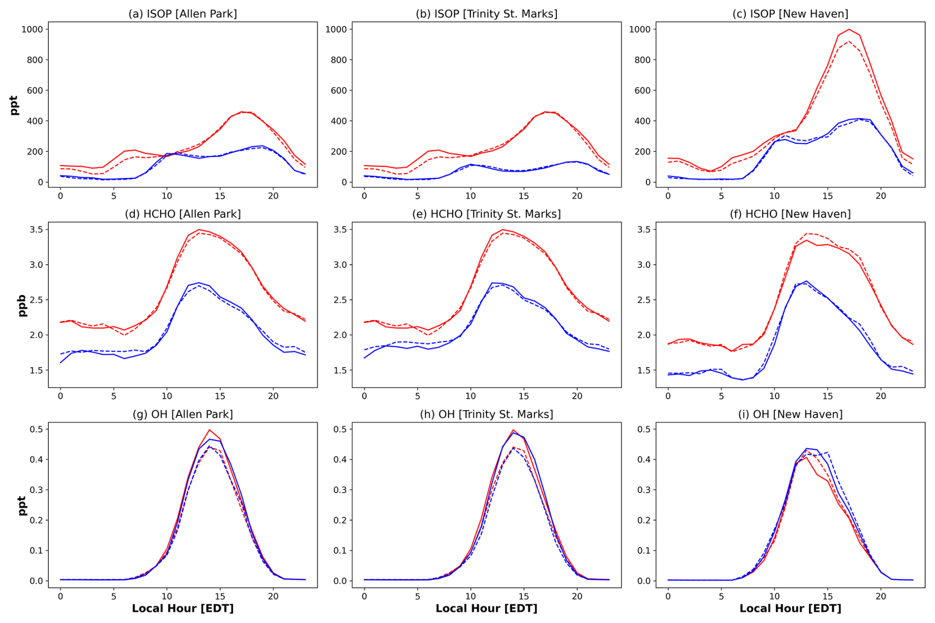
Figure 18 Same as Fig. 15 but for isoprene (ISOP), formaldehyde (HCHO), and the hydroxyl radical (OH).

The findings of this study show that O₃ production in SEMI is strongly governed by the spatial distribution of emissions and different chemical regimes. The urban location analysis showed that Detroit, which is a major industrial hub in the region, is consistent with a VOC-limited regime, where O₃ concentrations are suppressed by high NO_x titration in the daytime but can become sensitive to changes in VOCs during peak O₃ times. The suburban and remote location analysis (i.e., Allen Park and New Haven, respectively) showed that they are in a more NO_x-limited regime, where higher BVOCs and lower NO_x titration can lead to more efficient O₃ production. The spatial distribution is seen more clearly as we move towards finer resolutions, indicating more realistic emissions.

In VOC-limited regimes, targeting reductions in VOCs, such as those from the industrial sectors, is crucial compared to reductions in NO_x, as it could lead to temporary increases in O₃ production. In NO_x-limited regimes, where NO₂ drives O₃ production, reductions in transportation emissions and long-range transport would decrease O₃. The improvement in model representation of NO₂ and, in turn, O₃ during rush hour times (Figs. 4–5) shows how emissions can be misrepresented in the models. It is necessary that future work considers incorporating higher-resolution temporal profile and regional emissions to better distinguish different O₃ processes. Future work should also explore the impacts of targeting the contribution of different emission scenarios in SEMI to demonstrate the impact of different regulatory decision-making outcomes.

5 Conclusions

Tropospheric O₃ in SEMI is a persistent problem in the region, majorly resulting from anthropogenic activity. MUSICAv0, a global chemistry–climate model with regional refinement capabilities, has allowed us to evaluate whether the MUSICA framework is suitable for studying O₃ atmospheric chemistry in local, urban environments. This study aimed to evaluate the impact of horizontal grid resolution and diurnal cycles (for anthropogenic NO emission) on MUSICAv0 simulations, using a custom grid over the state of Michigan with a resolution of $\mathrm{1}/\mathrm{16}$° and leveraging a suite of measurements from Phase I of the MOOSE field campaign in 2021.

For O₃ and its precursors, both grid resolution and the diurnal cycle for anthropogenic NO emissions were important, largely depending on the time of day and the region. Horizontal grid resolution was important for O₃ during peak O₃ times (12:00–18:00 EDT), but during the night and early morning, O₃ was largely impacted by the application of the diurnal cycle as a result of changing NO₂ during NO_x peak times.

This work compares simulated NO₂ and HCHO tropospheric columns from MUSICAv0 model runs to measurements from the Pandora network at two sites in SEMI for the first time. The NO₂ columns from Pandora agreed with the temporal variability of the NO₂ columns at the two urban sites, where the application of the diurnal cycle for anthropogenic NO emissions at both resolutions generally made the model perform better during peak NO₂ times but resulted in greater model overestimations in the later part of the day. These trends are important because they can be indicative of high anthropogenic emission sources from industry and transportation in the model. Modeled HCHO columns compared to Pandora, on the other hand, were largely impacted by a combination of grid resolution and the diurnal cycle, where grid resolution impacts HCHO because of online calculations of biogenic VOCs and changing NO_x levels can promote VOC oxidation, leading to lower HCHO columns in the model. These changes led to underestimations of HCHO tropospheric columns in the model compared to the observations. This underestimation indicates that the model simulations are not capturing anthropogenic VOCs efficiently.

In addition,the NO₂ tropospheric columns from the model simulations were compared to observations from GCAS for the first time. This comparison showed that the finer resolution captured more pronounced pollution plumes corresponding to observed wind directions, which can be important when assessing transport from more localized sources. As the grid resolution in global chemistry–climate models becomes finer, future work should consider using NO₂ column data from remote sensing instruments to develop regional emission inventories for more fine-scale applications.

This work showed that grid resolution is more important for O₃ precursors (i.e., NO_x, HCHO, isoprene) than for O₃ itself, which agrees with the findings in Jo et al. (2023) and Schwantes et al. (2022). Changes due to grid resolution were largely a result of the artificial mixing of emissions. Finer resolutions can better classify source regions and distinguish between urban and non-urban regions. Grid resolution also impacted biogenic VOCs, as they are calculated online via MEGANv2.1 based on various meteorological parameters. Although isoprene in the finer-resolution simulations showed better performance compared to the AML measurements, SEMI is generally not prone to high isoprene emissions. Future work using the regional refinement grid over Michigan should focus on evaluating locations with higher vegetation density.

Applying diurnal cycles for anthropogenic NO on monthly emissions also played a crucial role in nighttime O₃ chemistry. The diurnal cycle often impacted O₃ and precursor concentrations more than the grid resolution. Future work should evaluate the impacts of applying diurnal cycles to more anthropogenic emissions other than NO. In addition, we acknowledge that apart from applying a diurnal cycle for anthropogenic NO emissions, the evolution of the PBL can also play a significant role in the formation of O₃ and NO_x. In the daytime, a rising PBL can mix surface NO_x and VOCs upwards, reducing O₃ concentrations near the surface, while in the nighttime, a shallower PBL can trap emissions near the surface, leading to higher NO_x titration. Uncertainties associated with the PBL could lead to underpredictions of NO₂ in the model and misrepresentations of O₃ peaks.

This is one of a few studies evaluating O₃ production and loss processes with custom grids in MUSICAv0. Although O₃ biases still persist in the MUSICAv0 simulations over this region, these biases are generally lessened with finer grid resolution during peak O₃ times and with diurnal cycles for anthropogenic NO during the nighttime. This case study is limited to SEMI, which can have different implications compared to previous work. For example, the state of Michigan is about 2.5 times larger than South Korea, which was studied in Jo et al. (2023) using a similar methodology, and has a completely different topography. Michigan is generally flat and surrounded by freshwater lakes, as opposed to South Korea's mountainous terrain surrounded by ocean encompassing a megacity. Schwantes et al. (2022) found that O₃ was better simulated over urban regions across the Southeastern US, especially when using a ∼ 14 km regional refinement grid and updated chemistry in MUSICAv0. This work took into consideration a finer grid resolution mesh (∼ 7 km) and compared to ∼ 14 km to show that regional refinement improves O₃ representativeness in the model. Future work aims to take advantage of custom grids to quantify the contribution of emissions and transport to O₃ atmospheric chemistry in the region. Future work should also take into consideration the use of a more updated version of the CAMS-GLOB-ANT emissions, as well as the diurnal variation profiles of CAMS-GLOB-TEMPO (Guevara et al., 2021; Soulie et al., 2024), or more regional emission inventories such as the National Emission Inventory (NEI) from the US EPA. Optimization of a regionally refined, coupled model such as MUSICAv0, through resolution and emission modeling studies, can have significant implications for the design and development of effective surface O₃ mitigation strategies in SEMI.