A new vertical reduction model for enhancing the interpolation accuracy of VMF1/VMF3 tropospheric delay products

Grid-wise Vienna Mapping Functions 1 (VMF1) and Vienna Mapping Functions 3 (VMF3) tropospheric products are widely used to interpolate the a priori zenith hydrostatic delay (ZHD) and zenith wet delay (ZWD) over GNSS (Global Navigation Satellite Systems) stations for the mitigation of tropospheric delays contained in GNSS observations. Since these two products provide ZHD and ZWD values only for the ground surface at global grid points, the ZHD and ZWD at the four grid points nearest to a GNSS site used to interpolate for the GNSS site need to be reduced to the same height of the GNSS station before a horizontal interpolation (e.g., bilinear interpolation) is implemented. However, the accuracy of the officially recommended reduction model may not be as good as desired, especially in the case that the height of the GNSS site largely differs from that of the four ground grid points. To address this, a new vertical reduction model for reducing the ZHD and ZWD at the height of grid points to a target height was developed. The sample data for the modelling were the 10-year (2010–2019) ZHD and ZWD profiles over grid points obtained from ERA5 monthly averaged reanalysis data, while the 3-year (2020–2022) radiosonde profiles and the IGS (International GNSS Service) site-wise zenith tropospheric delay (ZTD) products were used to evaluate the new model. Results demonstrated that the accuracy of ZHD, ZWD, and consequently ZTD values interpolated from VMF1/VMF3 products and the new model considerably improved compared to traditional methods, especially at the target sites that have large height differences from its closest VMF grid points. This improvement has significance for those applications that need to use tropospheric delay corrections, e.g. in GNSS positioning and GNSS meteorology for a desired accuracy.

1 Introduction

Tropospheric delay arises when electromagnetic waves propagate through the Earth's atmosphere and are refracted by neutral gases, which is defined as:

$$\begin{array}{}\text{(1)}& \mathrm{TD}={\mathrm{10}}^{-\mathrm{6}}\int N\mathrm{d}s+(\int \mathrm{d}s-L)\end{array}$$

where the first term represents the delay caused by the change in signal velocity along the actual (bent) propagation path s; the second term accounts for the geometric path difference along the straight satellite–receiver line L; N is the atmospheric refractivity (dimensionless):

$$\begin{array}{}\text{(2)}& \begin{array}{rl}N& =k_{\mathrm{1}}\cdot {\displaystyle \frac{P_{\mathrm{d}}}{T}}+\left(k_{\mathrm{2}}\cdot {\displaystyle \frac{e}{T}}+k_{\mathrm{3}}\cdot {\displaystyle \frac{e}{T^{\mathrm{2}}}}\right)\\ & =k_{\mathrm{1}}\cdot {\displaystyle \frac{P}{T}}+\left(k_{\mathrm{2}}^{\prime }\cdot {\displaystyle \frac{e}{T}}+k_{\mathrm{3}}\cdot {\displaystyle \frac{e}{T^{\mathrm{2}}}}\right)=N_{\mathrm{h}}+N_{\mathrm{nh}}\end{array}\end{array}$$

where k₁, k₂, k₃ are three refractivity constants (Rüeger, 2002; Thayer, 1974); P_d and e are atmospheric pressures (in hPa) resulting from dry air and water vapor, respectively; P is the total atmospheric pressure ($P=P_{\mathrm{d}}+e$); T is the atmospheric temperature (in K); N_h and N_nh are hydrostatic and non-hydrostatic part of the refractivity, respectively. $k_{\mathrm{2}}^{\prime }$ is a constant related to k₁ and k₂:

$$\begin{array}{}\text{(3)}& k_{\mathrm{2}}^{\prime }=k_{\mathrm{2}}-k_{\mathrm{1}}{\displaystyle \frac{R_{\mathrm{d}}}{R_{\mathrm{v}}}}\end{array}$$

where R_d and R_v are the specific gas constants for dry air and water vapor, respectively. $R_{\mathrm{d}}=R/M_{\mathrm{d}}$,$R_{\mathrm{v}}=R/M_{\mathrm{v}}$, where R is the universal gas constant (8.3143 J K⁻¹ mol⁻¹); M_d (28.9644 g mol⁻¹) and M_w (18.0152 g mol⁻¹) are the molar mass of dry air constant and water, respectively.

The tropospheric delay is one of the major error sources embedded in observations of space geodetic techniques, such as GNSS (Global Navigation Satellite Systems) and VLBI (Very Long Base-line Interferometry). The second term in Eq. (1), which represents the geometric path change, is typically quite smaller than the first term (usually less than 0.1 mm for elevation angles above 57°). Moreover, the bending effect is generally accounted for using advanced mapping functions (see Eq. 5) (Möller and Landskron, 2019; Nafisi et al., 2012) . Therefore, most research efforts focus on modelling the first term in Eq. (1), which dominates the total delay. As a convention, the zenith tropospheric delay (ZTD) is widely used in GNSS and VLBI data processing:

$$\begin{array}{}\text{(4)}& \mathrm{ZTD}=\int N_{\mathrm{h}}\mathrm{d}h+\int N_{\mathrm{nh}}\mathrm{d}h=\mathrm{ZHD}+\mathrm{ZWD}\end{array}$$

where ZHD and ZWD are zenith hydrostatic delay and zenith non-hydrostatic delay (also known as zenith wet delay (ZWD)), respectively. Then a slant tropospheric delay can be modelled using ZHD, ZWD together with mapping functions (Chao, 1974; Chen and Herring, 1997; Niell, 1996):

$$\begin{array}{}\text{(5)}& \mathrm{TD}=\mathrm{ZHD}\cdot {\mathrm{mf}}_{\mathrm{h}}+\mathrm{ZWD}\cdot {\mathrm{mf}}_{\mathrm{w}}+\mathrm{\Delta }{T}_{\mathrm{grad}}\end{array}$$

where mf_h and mf_w are the mapping functions for the hydrostatic and non-hydrostatic part of the tropospheric delay, respectively; ΔT_grad is the tropospheric gradient, which is caused by the azimuthal asymmetry of the troposphere.

Given the distinct dynamic characteristics of the ZHD and ZWD, GNSS data processing typically applies a correction for the ZHD using external models or products, while treating the ZWD as an unknown parameter to be estimated. Due to differences between the hydrostatic and wet mapping functions, the error in ZHD cannot be absorbed into the estimated ZWD completely. This discrepancy can subsequently degrade the accuracy of both the ZTD and station height estimates (Boehm et al., 2006; Tregoning and Herring, 2006; Kouba, 2009). Moreover, accurate ZHD is crucial in GNSS meteorology, where ZTD is converted to precipitable water vapor (Bevis et al., 1992; Wang et al., 2017; Zhu et al., 2024). A 1 cm error in ZHD can introduce an error of approximately 1.5 mm in the retrieved precipitable water vapor (PWV). For ZWD, pre-obtained values can be used directly to correct the wet delay or treated as pseudo-observations to constrain the estimation of the wet delay, thereby accelerating the convergence of precise point positioning (PPP) solutions (Sun et al., 2021a). Therefore, improving the accuracy of ZHD and ZWD has been a long-standing global effort in the advancement of space geodetic data processing.

The ZHD can be modeled with high accuracy using the Saastamoinen model, provided that in-situ atmospheric pressure (P) measurements are available (Davis et al., 1985; Saastamoinen, 1972):

$$\begin{array}{}\text{(6)}& \begin{array}{rl}\mathrm{ZHD}& ={\displaystyle \frac{\mathrm{0.0022768}P}{f(\mathit{\phi },H)}}\\ & ={\displaystyle \frac{\mathrm{0.0022768}P}{\mathrm{1}-\mathrm{0.00266}\cos \left(\mathrm{2}\mathit{\phi }\right)-\mathrm{0.00028}H}}\end{array}\end{array}$$

where φ and H are the latitude (in radians) and height (in km) of the GNSS site, respectively. Although the ZWD can also be calculated using empirical models such as the Askne-Nordius model (Askne and Nordius, 1987), which relies on in-situ meteorological measurements (e.g., water vapor pressure), its accuracy is generally lower than that of the ZHD model. This is primarily because water vapor exhibits high spatial variability, even when precise in-situ measurements are available (Chen and Liu, 2016).

Since most GNSS stations are not mounted with meteorological sensors and it is computationally complex for real-time GNSS users to process forecasted numerical weather model (NWM) data to obtain the atmospheric parameters, empirical tropospheric delay models are widely used alternatives. Among the most commonly adopted models are the UNB3m model (Leandro et al., 2006) developed by the University of New Brunswick (UNB) and the Global Pressure and Temperature (GPT) model series developed by the Vienna University of Technology (TU Wien). These models operate independently of external meteorological inputs and empirically estimate atmospheric parameters (such as atmospheric pressure, water vaper pressure, temperature, etc.) based solely on a given location and time. The UNB3m model uses lookup tables that provide the mean and annual amplitude of meteorological variables at mean sea level, facilitating tropospheric delay computation through standardized vertical reduction models. Boehm et al. (2007) introduced the first version of the GPT model, which represents global atmospheric pressure and temperature using spherical harmonics. Its successor, GPT2 (Lagler et al., 2013) advanced the GPT series by implementing a global 5° × 5° grid and characterizing atmospheric pressure, temperature, temperature lapse rate, and water vapor pressure by accounting for their mean, annual, and semi-annual harmonics. The GPT2w model (Böhm et al., 2015) refined this framework by incorporating additional parameters and increasing the resolution to 1° × 1°. The GPT3 (Landskron and Böhm, 2018) integrated an empirical gradient model while maintaining the other meteorological parameters consistent with GPT2w. Both the UNB3m and GPT model series furnish meteorological parameters at a single reference level (either mean sea level or Earth's surface), necessitating their vertical propagation to the desired elevation. To enhance the accuracy of tropospheric delay modelling, recent studies have introduced more advanced modelling techniques that better describe the height-dependent variability of atmospheric parameters (Huang et al., 2023; Jiang et al., 2024; Li et al., 2018; Sun et al., 2023). Nevertheless, while these empirical models can predict atmospheric parameters with reasonable accuracy, they are fundamentally limited to capturing long-term average variations, primarily annual and semi-annual cycles. As a result, their predictive accuracy is inherently constrained by the atmosphere's continuous and often abrupt variability, particularly for rapidly fluctuating parameters such as air temperature and water vapor pressure (Wang et al., 2017; Xia et al., 2023).

Fortunately, the tropospheric delay can also be obtained from grid-wise Vienna Mapping Functions 1 (VMF1) (Boehm et al., 2006, 2009) and Vienna Mapping Functions 3 (VMF3) (Landskron and Böhm, 2018) products provided by TU Wien. The grid-based VMF1 product has a horizontal resolution of 2.5° × 2°, while the VMF3 product offers resolutions of 1° × 1° and 5° × 5°. For each grid point, the ZHD, ZWD, and mapping function coefficients are computed at four epochs (00:00, 06:00, 12:00, 18:00 UTC) per day using NWM data from the European Centre for Medium-Range Weather Forecasts (ECMWF). These products allow tropospheric delays for any specific time and location to be obtained via interpolation from surrounding grid points. Two types of NWM data are used to generate the VMF1/VMF3 products, i.e., ECMWF OPERATIONAL NWM for VMF1_OP and VMF3_OP, and ECMWF FORECAST NWM for VMF1_FC and VMF3_FC. In addition, some other VMF1-like products are also publicly available for users (Zus et al., 2015).

Recent studies have shown that the accuracy of the tropospheric delays obtained from the grid-wise VMF1 and VMF3 products are considerably better than those predicted by the above-mentioned empirical models (Sun et al., 2021b; Yang et al., 2021). Prior to the release of VMF3, the VMF1 product was highly recommended for GNSS data processing (Kouba, 2008). Yao et al. (2018b) evaluated the ZTD predicted by VMF1_FC using references from IGS (International GNSS Service) final ZTD products and results demonstrated a mean root-mean-square (RMS) of 1.83 cm. Yuan et al. (2019) assessed the performance of VMF1_FC in real-time precise point positioning (PPP) and found that the accuracy of PPP-derived positions and ZTDs was superior when using ZHD values from VMF1_FC compared to empirical models. The VMF3 product, offering resolutions of 1° × 1° and 5° × 5°, have become available since 2018, and its associated mapping function has been shown to outperform that of VMF1 (Landskron and Böhm, 2018). Sun et al. (2021a) utilized ZWD values predicted by VMF3_FC (1° × 1°) as a pseudo-observation to constrain the ZWD parameter in real-time single-frequency (SF) PPP, demonstrating that the convergence time of SF-PPP was considerably shortened. Yang et al. (2021) evaluated the accuracy of the ZHD and ZWD values predicted by VMF3_OP across China using reference data from ERA5 reanalysis. Sun et al. (2021b) evaluated the accuracy of the ZHD predicted by VMF1_FC and VMF3_FC using 3-year surface atmospheric pressures measured at 443 globally distributed radiosonde stations and results showed that the mean RMSE of the ZHD values predicted by VMF1_FC, VMF3_FC (5° × 5°) and VMF3_FC (1° × 1°) at all the 443 stations were 5.9, 5.4, and 4.3 mm, respectively.

While ZTD values derived from VMF1 and VMF3 products generally exhibit superior accuracy compared to those derived from empirical tropospheric models, notable errors in ZHD and ZWD under certain conditions have been reported in several studies (Sun et al., 2021b; Yang et al., 2021; Yao et al., 2018b). In particular, the RMSE of ZHD estimated using grid-wise VMF1/VMF3 data with the officially recommended interpolation method can reach up to 5 cm when compared with reference ZHD values obtained from radiosonde measurements in certain regions (Sun et al., 2021b). Similarly, the RMSE of ZWD can also reach substantial magnitudes (Sun et al., 2021a; Yang et al., 2021). These findings highlight the potential limitations of existing interpolation methods, particularly in regions characterized by complex terrain. To address this issue and improve the accuracy of ZTD interpolated from VMF1/VMF3 products, this study re-evaluates the conventional interpolation strategy and introduces a new vertical reduction model. This model provides grid-wise vertical reduction coefficients for ZHD and ZWD at each VMF grid point, enabling more accurate height-related adjustments prior to horizontal interpolation. The methodology and data utilized in this research are presented first, followed by test results, their analyses, and discussion. Conclusions are summarized in the final section.

2 Data Sources

2.1 ERA5 monthly averaged reanalysis data

ERA5 reanalysis data are the state-of-the-art atmospheric reanalysis data provided by the ECMWF. In this contribution, the 10 years (2010–2019) of ERA5 monthly averaged reanalysis data, including geopotential, temperature and water vapor pressure at 37 pressure levels over the grid points of VMF1 and VMF3 products were selected as the samples for the development of the new ZTD vertical reduction model. To adapt to geodetic applications, the geopotential heights were converted to ellipsoidal heights using the transformation equations described by Nafisi et al. (2012).

2.2 Radiosonde data

For the evaluation of the newly developed ZHD and ZWD vertical reduction models, atmospheric profiles from 608 radiosonde stations in the 3-year period of 2020–2022 were selected for the calculation of references. The selection was based on the criterion that the station observed at least 500 valid profiles during the 3-year period to ensure temporal continuity. The geographical distribution of these finally selected stations is illustrated in Fig. 1a. The reference ZHD and ZWD were obtained using discrete integration form of Eq. (4) (Andrei and Chen, 2009; Askne and Nordius, 1987):

$$\begin{array}{}\text{(7)}& \begin{array}{rl}& \mathrm{ZHD}=\sum N_{\mathrm{h}}\mathrm{d}h\\ & \mathrm{ZWD}=\sum N_{\mathrm{nh}}\mathrm{d}h\end{array}\end{array}$$

2.3 GNSS-ZTD data

ZTD products in the 3-year period of 2020–2022 at 394 IGS stations were used to evaluate the new ZHD and ZWD vertical reduction models. A rigorous quality control procedure was implemented to ensure the quality of these reference ZTDs. Initially, the IGS-ZTD time series, originally at 5 min intervals, was resampled to a 2 h interval. To mitigate the impact of known midnight discontinuities, present in the IGS-ZTD time series, only odd-numbered UTC epochs (i.e., 1, 3, …, 23) were retained. Subsequently, epochs with a standard deviation exceeding 4 mm, as indicated within the IGS-ZTD products, were excluded. Consequently, those stations that had less than 5000 ZTD epochs were removed, and the number of the remained stations was 394, see the geographical distribution of these stations in Fig. 1b.

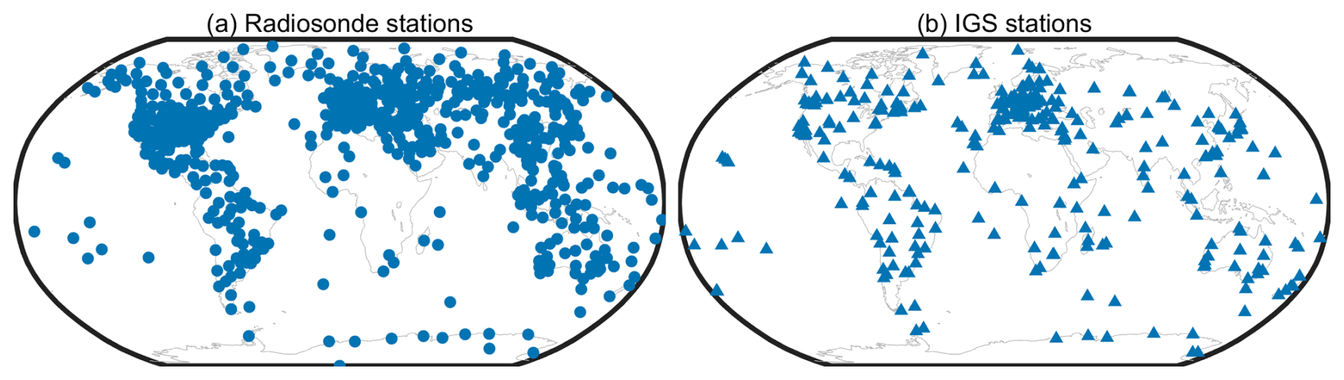
Figure 1 Geographical distribution of (a) 608 radiosonde stations and (b) 394 IGS stations selected for the evaluation of the new model.

3 Methodology

3.1 Officially recommended ZTD interpolation method

The officially recommended ZTD interpolation method is examined in this section for the analysis of improvements to be made in the accuracy of VMF1/VMF3-predicted ZTD. Its procedure is as follows.

1. Identifying the four ground grid points surrounding the target point S (see Fig. 2) provided in the VMF1 and VMF3 products, see points A–D. Then, for each grid point, the following procedure is performed.

2. Performing a linear interpolation for the ZHD and ZWD values of the grid point in the temporal domain: data from the two neighbouring epochs (selected from 00:00, 06:00, 12:00, 18:00 UTC) that are closest to S are used in the interpolation, and the interpolated results are denoted by ZHD₀ in Eq. (8) and ZWD₀ in Eq. (10) since they are the ground surface value at one of A–D.

3. Using an inverse process of Eq. (6) to calculate the ground atmospheric pressure of the grid point:

   $$\begin{array}{}\text{(8)}& P_{\mathrm{0}}={\displaystyle \frac{{\mathrm{ZHD}}_{\mathrm{0}}\left[\mathrm{1}-\mathrm{0.00266}\cos \left(\mathrm{2}\mathit{\phi }\right)-\mathrm{0.00028}{h}_{\mathrm{0}}\right]}{\mathrm{0.0022768}}}\end{array}$$

   where P₀ and h₀ are the ground atmospheric pressure and height of the grid point, respectively.

4. Reducing P₀ to the height of S using the following vertical atmospheric pressure reduction model (Kouba, 2008):

   $$\begin{array}{}\text{(9)}& P=P_{\mathrm{0}}{\left(\mathrm{1}-\mathrm{0.0000266}\mathrm{\Delta }h\right)}^{\mathrm{5.225}}\end{array}$$

   where P is the reduced atmospheric pressure at the height of S (A'–D'); 0.0000266 is an empirical decay parameter for atmospheric pressure; Δh is the difference between the target and reference heights, i.e. $\mathrm{\Delta }{h}_{{\mathrm{AA}}^{\prime }}$ , $\mathrm{\Delta }{h}_{{\mathrm{BB}}^{\prime }}$, $\mathrm{\Delta }{h}_{{\mathrm{CC}}^{\prime }}$, $\mathrm{\Delta }{h}_{{\mathrm{DD}}^{\prime }}$.

5. Using Eq. (6) with the input of P obtained in Eq. (8) to obtain reduced ZHD for the grid point.

6. Using ZWD₀ (i.e., ground) and the following model to obtain ZWD for the height of S for the grid point:

   $$\begin{array}{}\text{(10)}& \mathrm{ZWD}={\mathrm{ZWD}}_{\mathrm{0}}\cdot \exp \left({\displaystyle \frac{-\mathrm{\Delta }h}{\mathrm{2000}}}\right)\end{array}$$

7. Repeating steps (2)–(6) for all the four points (A'–D'), then using the four reduced ZHD and ZWD values and the bilinear interpolation in the spatial domain to obtain the interpolated ZHD and ZWD for the position of S.

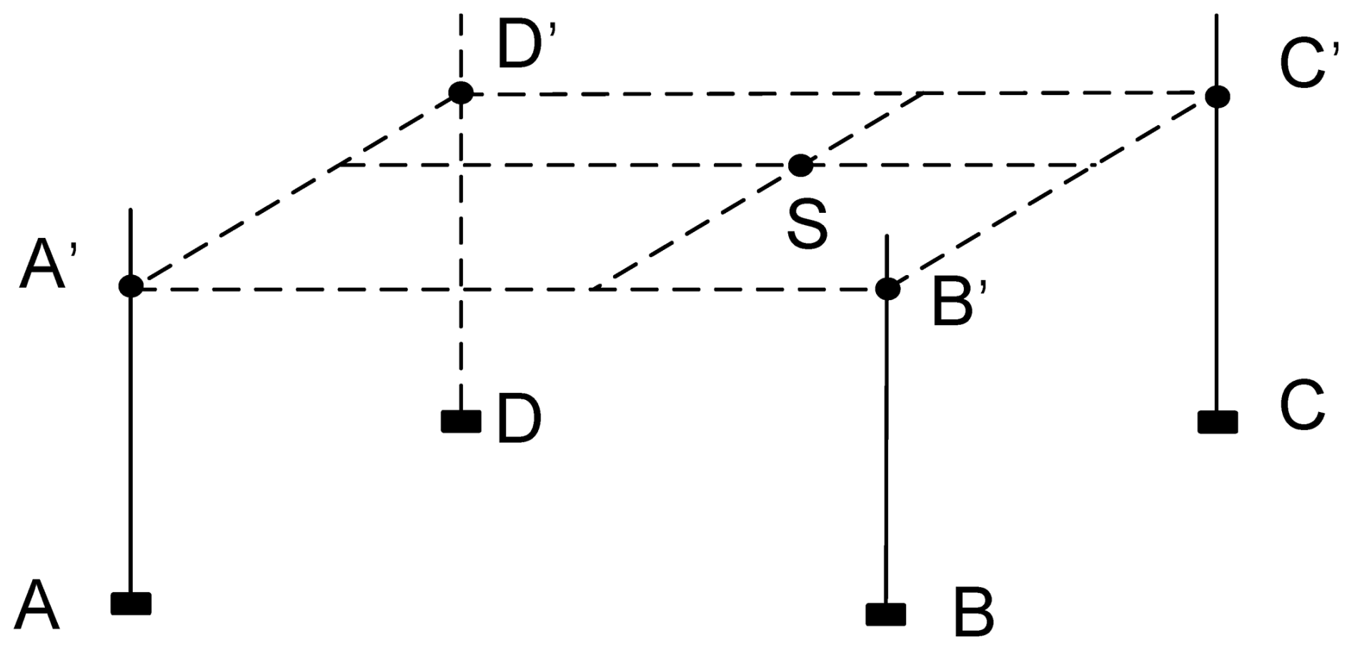
Figure 2 ZHD and ZWD at the position of S are obtained by an interpolation of the ZHD and ZWD values at the four ground grid points surrounding S (A to D), then reduced to the height of S (A'–D').

3.2 GPT2w-based ZTD reduction method

It is noted that in Eq. (9), a fixed empirical value 0.0000266 is used for the atmospheric pressure decay parameter on a global scale. However, due to the spatio-temporal variations in atmospheric pressure (Wang et al., 2022; Zhang et al., 2021a), the vertical reduction model may not perform well. Therefore, taking into account the spatio-temporal variations in atmospheric pressure models is most likely to improve their accuracy. For example, Eq. (9) can be replaced with:

$$\begin{array}{}\text{(11)}& P=P_{\mathrm{0}}{\left(\mathrm{1}-{\displaystyle \frac{\mathit{\beta }}{T_{\mathrm{0}}}}\mathrm{\Delta }h\right)}^{\frac{g_{\mathrm{m}}\cdot M_{\mathrm{d}}}{R\cdot \mathit{\beta }}}\end{array}$$

where T₀ is the temperature (in K) at the reference height; β is the temperature lapse rate; g_m is the mean gravitational acceleration. The accuracy of T₀ and β determines the accuracy of the vertical reduction function. Fortunately, these two values can be obtained from empirical models e.g. GPT2w. Zhang et al. (2021b) utilized GPT2w-predicted atmospheric temperature and its lapse rate as the input of Eq. (11) for the vertical reduction to the ZHD provided by VMF1/VMF3-like products, and test results in the Tibetan Plateau region showed considerable improvements.

In this research, the water vapor decrease factor (λ) predicted by GPT2w was applied to the vertical reduction for the ZWD provided in grid-wise VMF1/VMF3 products using the following ZWD decay function given by Dousa and Elias (2014):

$$\begin{array}{}\text{(12)}& \mathrm{ZWD}={\mathrm{ZWD}}_{\mathrm{0}}{\left(\mathrm{1}-{\displaystyle \frac{\mathit{\beta }}{T_{\mathrm{0}}}}\mathrm{\Delta }h\right)}^{\frac{(\mathit{\lambda }+\mathrm{1})\cdot g_{\mathrm{m}}}{R_{\mathrm{d}}\cdot \mathit{\beta }}}\end{array}$$

3.3 A new ZTD reduction method for VMF1/VMF3 products

If a constant temperature lapse rate (β=0.0065 K m⁻¹) is utilized, the exponential term of Eq. (11). can be simplified as (Yao et al., 2018a):

$$\begin{array}{}\text{(13)}& P=P_{\mathrm{0}}{\left[\mathrm{1}-\mathit{\tau }\left(h-h_{\mathrm{0}}\right)\right]}^{\mathrm{5.256}}\end{array}$$

where $\mathit{\tau }=\mathit{\beta }/T_{\mathrm{0}}$. Since the denominator part of Eq. (6), i.e., f(φ,H) in Eq. (6), is close to 1, the specific value of the ZHD at height h above the reference height can be simplified as:

$$\begin{array}{}\text{(14)}& {\displaystyle \frac{\mathrm{ZHD}}{{\mathrm{ZHD}}_{\mathrm{0}}}}={\displaystyle \frac{P_{\mathrm{0}}{\left[\mathrm{1}-\mathit{\tau }\left(h-h_{\mathrm{0}}\right)\right]}^{\mathrm{5.256}}}{P_{\mathrm{0}}}}\end{array}$$

Then the ZHD at height h can be obtained by:

$$\begin{array}{}\text{(15)}& \mathrm{ZHD}={\mathrm{ZHD}}_{\mathrm{0}}{\left[\mathrm{1}-\mathit{\tau }\left(h-h_{\mathrm{0}}\right)\right]}^{\mathrm{5.256}}\end{array}$$

The ZWD decay function proposed by Dousa and Elias (2014) was utilized in this study:

$$\begin{array}{}\text{(16)}& {\displaystyle \frac{\mathrm{ZWD}}{{\mathrm{ZWD}}_{\mathrm{0}}}}={\left({\displaystyle \frac{P}{P_{\mathrm{0}}}}\right)}^{\mathit{\gamma }+\mathrm{1}}\end{array}$$

where γ is the ZWD decay parameter.

Substituting Eq. (13) into Eq. (16) leads:

$$\begin{array}{}\text{(17)}& {\displaystyle \frac{\mathrm{ZWD}}{{\mathrm{ZWD}}_{\mathrm{0}}}}={\left[\mathrm{1}-\mathit{\tau }\left(h-h_{\mathrm{0}}\right)\right]}^{\mathrm{5.256}(\mathit{\gamma }+\mathrm{1})}\end{array}$$

Thus

$$\begin{array}{}\text{(18)}& \mathrm{ZWD}={\mathrm{ZWD}}_{\mathrm{0}}{\left[\mathrm{1}-\mathit{\tau }\left(h-h_{\mathrm{0}}\right)\right]}^{\mathrm{5.256}(\mathit{\gamma }+\mathrm{1})}\end{array}$$

In this study, τ and γ for each of VMF1/VMF3 grid points were modeled using the following procedure:

1. For the spatial domain, τ and γ at the ground surface of the grid point for the 120 months in the 10-year period of 2010–2019 were fitted using the ERA5 monthly averaged reanalysis data mentioned above.

2. For the temporal domain, the seasonal variation trends of τ and γ at the grid point fitting the above 120 monthly averaged τ and γ values were modelled by:

   $$\begin{array}{}\text{(19)}& \begin{array}{rl}t& =t_{\mathrm{0}}+A_{\mathrm{1}}\cos \left({\displaystyle \frac{\mathrm{DOY}-d_{\mathrm{1}}}{\mathrm{365.25}}}\mathrm{2}\mathit{\pi }\right)\\ & +A_{\mathrm{2}}\cos \left({\displaystyle \frac{\mathrm{DOY}-d_{\mathrm{2}}}{\mathrm{365.25}}}\mathrm{4}\mathit{\pi }\right)\end{array}\end{array}$$

   where t₀ is the mean of the parameter (i.e., either τ or γ); A₁ and A₂ are the amplitudes of annual and semi-annual variation of the parameter, respectively; d₁ and d₂ are the day of year (DOY) corresponding to their initial phase. Then the ZHD and ZWD at height h can be obtained using Eqs. (15) and (18), respectively.

4 Results and discussion

To compare the accuracies of the standard and alternative vertical reduction models for reducing the ground surface ZHD and ZWD from the grid reference height to target heights, the following three schemes were tested using ZHD and ZWD data obtained from grid-wise VMF1/VMF3 products.

1. Scheme 1. For the officially recommended reduction methods, which utilizes fixed empirical decay parameters, corresponding to Eq. (9) for ZHD and Eq. (10) for ZWD.

2. Scheme 2. For the temperature-dependent pressure decay model (Eq. 11) and the exponential ZWD decay model (Eq. 12). The required atmospheric variables, including temperature (T₀), temperature lapse rate (β), and water vapor decay coefficient (λ), are predicted by the GPT2w model.

3. Scheme 3. For the new vertical reduction model developed in this research, i.e., Eq. (15) for ZHD and Eq. (18) for ZWD.

   The RMSE was used to measure the overall accuracy of results obtained from the above three schemes:

   $$\begin{array}{}\text{(20)}& \mathrm{RMSE}=\sqrt{{\displaystyle \frac{\mathrm{1}}{n}}\sum _{i=\mathrm{1}}^n{\left({\mathrm{ZTD}}_{\mathrm{VMF},i}-{\mathrm{ZTD}}_{\mathrm{ref},i}\right)}^{\mathrm{2}}}\end{array}$$

   where ZTD_VMF and ZTD_ref are the VMF-based ZTD (or ZHD, ZWD) and the reference ZTD (or ZHD, ZWD), respectively. It should be noted that only the forecast VMF1/VMF3 products were utilized for the model evaluation since only these two products could be adapted to real-time GNSS data processing and real-time retrieval of PWV in GNSS meteorology.

4.1 Using radiosonde-ZTD as reference

In this section the ZHD and ZWD obtained from the 3-year (2020–2022) radiosonde profiles at eight pressure levels at the aforementioned 608 radiosonde stations were used as the reference.

Figure 3a (the top row) shows each scheme's mean RMSE of ZHD interpolated from VMF1 and VMF3 (with three spatial resolutions) at each pressure level in the 3-year period at all the 608 stations. We can see that Scheme 2 outperforms Scheme 1 at the three lowest levels (i.e. 1000, 925 and 850 hPa). However, at all the rest height levels Scheme 2 (blue) results are much worser than the other two, and the higher, the worser of its accuracy. Moreover, results from Scheme 3 (for the new model) were considerably better than the other two and its accuracies at different levels had little differences.

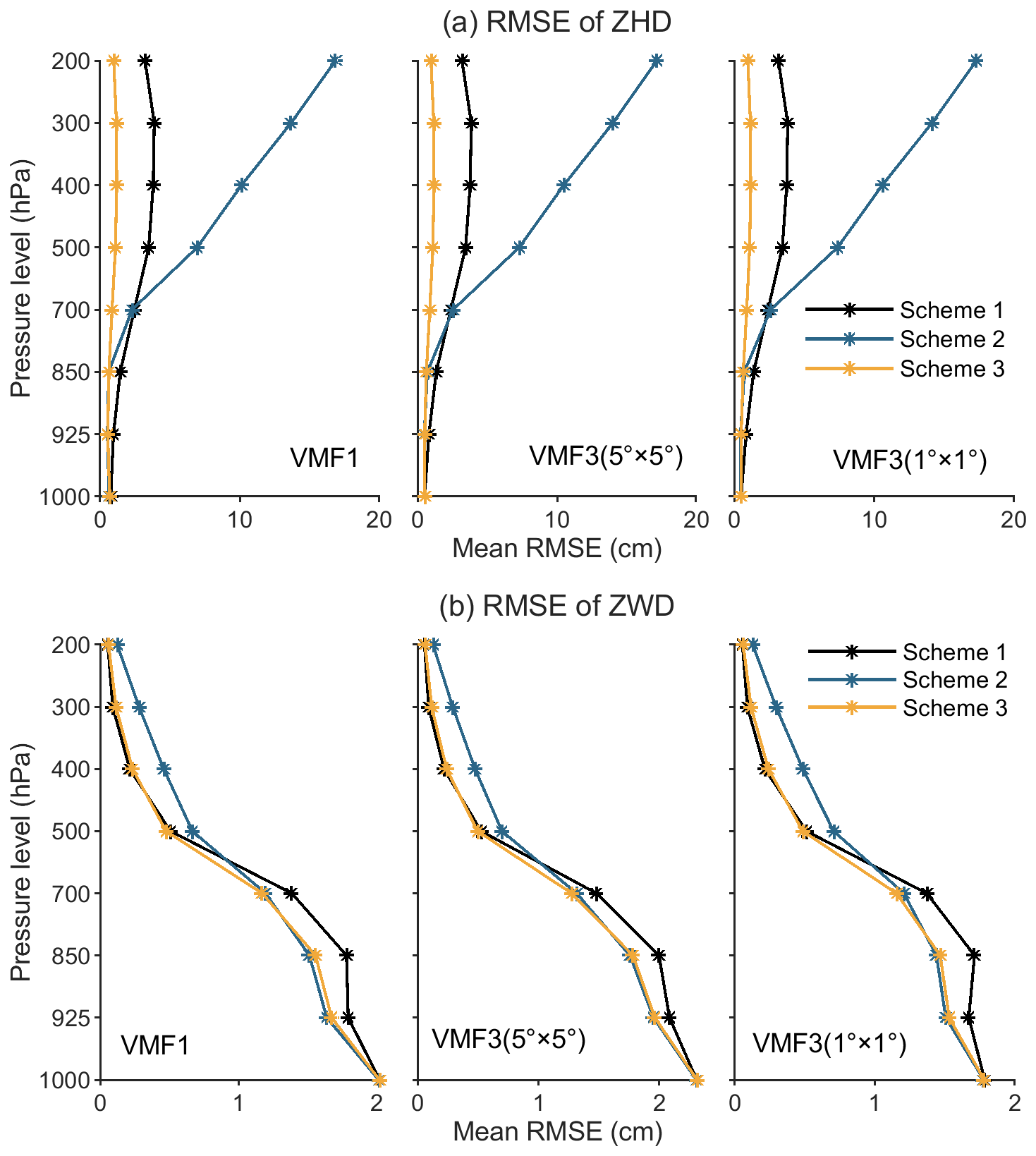
Figure 3 Mean RMSE of the (a) ZHD and (b) ZWD interpolated from VMF1_FC and VMF3_FC for each scheme at each pressure level in the 3-year (2020–2022) period at 608 radiosonde stations.

From Fig. 3b, which is for the results of the interpolated ZWD, we can see that Scheme 3 is also the best performer. Furthermore, at low levels, e.g. below 500 hPa, where the water vapor content mainly concentrates, Scheme 1 (black) is the worst, and Schemes 2 and 3 perform similarly. However, at the rest four levels (high), Schemes 1 and 3 had little differences, while Scheme 2 is the worst.

To summarize the above results, Scheme 3 (i.e. our new model) is the best in reducing the ZWD obtained from the grid-wise VMF1/VMF3 products, while Scheme 2 may offer an improved result only at low-altitude pressure levels in comparison with Scheme 1 (the officially recommended one).

Table 1 Mean, minimum and maximum RMSE (in cm) of ZTD resulting from each scheme in the 3-year period studied at 394 IGS stations. The bold numbers are used to highlight the improvement in the maximum RMSE.

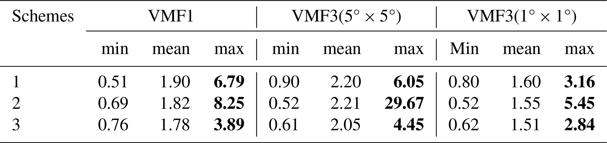
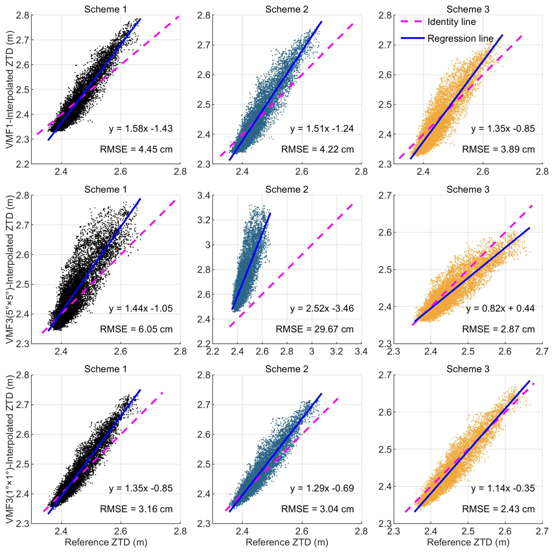
Figure 4 Correlation and accuracy analysis of ZTD interpolated from VMF1/VMF3 products and three schemes at IQQE station.

4.2 Using IGS-ZTD as reference

ZTD values at the aforementioned 394 IGS stations in the 3-year period studied were also used as the reference to evaluate the performance of the above three schemes. As introduced at the beginning of Sect. 4, these schemes represent different approaches to interpolating ZTD from gridded VMF data to station height.

Table 1 lists the mean, maximum and minimum RMSE values of the interpolated ZTDs from each scheme. One can observe that the maximum RMSE from Scheme  3 is considerably lower than those from Schemes 1 and 2, indicating that the proposed model enhances the interpolation accuracy of ZTD.

It should be noted that the IGS ZTD values are for ground surface and most IGS stations are located in relatively flat terrain, thus the mean RMSE of Scheme 3 was not notably smaller than that of the other two schemes. However, for those stations that ​are​ substantially higher or lower ​than​ ​their​ adjacent VMF grid points, the accuracy of interpolated ZTD for these stations was considerably improved. As an example, Fig. 4 shows the correlation and accuracy analysis of ZTD interpolated from VMF1/VMF3 products using three schemes at IQQE station. The IQQE (IGS network) station is located in Iquique, Chile (latitude: −20.273542°, longitude: −70.131717°, height: 38.9 m), which lies to the west of the Andes Mountains, thus this station exhibits substantial differences in height compared to its surrounding closest VMF1/VMF3 grid points: the maximum height differences reach 1562 m for VMF1, 4632 m for VMF3 (5° × 5°), and 2750 m for VMF3 (1° × 1°). As is shown in the figure, Scheme 3 consistently demonstrated the lowest ZTD RMSE among all three schemes and products. Specifically, for the VMF3 (5° × 5°) grid, the ZTD RMSE from Scheme 1 was 6.05 cm, while Scheme 2 resulted in a notably high RMSE of 29.67 cm, and RMSE value of the Scheme 3 was only 2.87 cm. The figure indicates a substantial influence of height differences between a GNSS station and its neighboring VMF1/VMF3 grid points on the interpolated ZTD (ZHD + ZWD), and the new model proposed in this research is strongly recommended in such cases.

5 Conclusions

The ZHD and ZWD provided by grid-based VMF1 and VMF3 tropospheric products are for ground surface values at each grid points, and these products have been widely used for interpolating the a priori ZHD and ZWD for GNSS positioning and VLBI stations. In the case that the height of the target GNSS station differs largely from its four surrounding grid points to be used for the interpolation of ZTD, the ZHD and ZWD values at the grid points need to be reduced to the height of the GNSS station before a horizontal interpolation is performed. Since traditional reduction models may not perform well in accuracy, in this study, new ZHD and ZWD reduction models for each of the four grid points to be used for interpolation were developed for an improvement in the accuracy of interpolated results. The sample data for the modeling were the ZHD and ZWD profiles over the grid points obtained from ERA5 monthly averaged reanalysis data during the period of 2010–2019. The two sets of reference data used to evaluate the new models were the ZHD and ZWD at eight pressure levels of radiosonde data at 608 stations and surface ZTD at 394 globally distributed IGS stations during the 3-year period 2020–2022. Test results showed that the accuracy of the ZHD, ZWD, as well as ZTD interpolated from the VMF1/VMF3 products reduced by the new model was considerably better than traditional methods. The new model is expected to be applied in fields such as GNSS positioning and GNSS-meteorology for better performance.