Impact of horizontal resolution and model time step on European precipitation extremes in the OpenIFS 43r3 atmospheric model

Events of extreme precipitation pose a hazard to many parts of Europe but are typically not well represented in climate models. Here, we evaluate daily extreme precipitation over Europe during 1982–2019 in observations (GPCC), reanalysis (ERA5), and a set of atmosphere-only simulations at low (100 km), medium (50 km), and high (25 km) horizontal resolution and also at different time steps (i.e., 60, 30, and 15 min) using low resolution (100 km) with identical vertical resolutions using OpenIFS (version 43r3). We find that both OpenIFS simulations and reanalysis underestimate the rates of extreme precipitation compared to observations. The biases are largest for the lowest resolution (100 km) and decrease with higher-horizontal-resolution (50 and 25 km) simulations in all seasons. The sensitivity to horizontal resolution is particularly high in mountain regions (such as the Alps, Scandinavia, Iberian Peninsula), likely linked to the sensitivity of vertical velocity to the representation of topography. The sensitivity of precipitation to model resolution increases dramatically with increasing percentiles, with modest biases in the 70th–80th percentile range and large biases above the 99th percentile range. We also find that precipitation above the 99th percentile mostly consists of large-scale precipitation (∼ 80 %) in winter, while in summer it is mostly large-scale precipitation in northern Europe (∼ 70 %) and convective precipitation in southern Europe (∼ 70 %). Convective precipitation is more sensitive to model time step than to horizontal resolution. Large-scale precipitation increases significantly with both higher horizontal resolution and a shorter model time step.

1 Introduction

Extreme precipitation events have severe impacts on our society and ecosystems. For example, extreme precipitation caused a devastating flood in Germany in 2021, in which around 180 people died. The frequency and intensity of extreme precipitation are projected to increase over most regions in the future (Intergovernmental Panel on Climate Change, 2023; Li et al., 2021; Myhre et al., 2019). The increasing extreme precipitation poses a threat to society and must thus be realistically simulated and projected accurately for future climates. However, climate models have large biases in simulating extreme precipitation events due to a coarse-horizontal-resolution grid and a long model time step (Alexander et al., 2019; Avila et al., 2015; Sillmann et al., 2013). The model biases are also hard to evaluate as we lack long-term observations. This study aims to understand the sensitivity of extreme precipitation to model horizontal resolution and model time step.

Extreme precipitation events are usually underestimated in Coupled Model Intercomparison Project (CMIP) models (O'Gorman, 2015; Sillmann et al., 2013). Some studies have found that simulated extreme precipitation at higher atmosphere horizontal resolutions is more realistic (Wehner et al., 2010, 2014). Jong et al. (2023) found that the characteristics of extreme precipitation at 25 km resolution configurations have smaller biases than at 50 and 100 km, while Kopparla et al. (2013) found that the reduced extreme precipitation biases at higher horizontal resolution do not hold for all regions (e.g., Australia). Strandberg and Lind (2021) reported that the effect of horizontal resolution on European extreme precipitation is largest in regions with complex topography and in the summer season when precipitation is mostly caused by convective processes using coupled models, in agreement with Iles et al. (2020). However, Li et al. (2011) demonstrated that the impact of horizontal resolution on global precipitation extremes is manifested mostly by its effects on large-scale precipitation, which could be due to the improved large-scale circulation (Hack et al., 2006). Other studies also found increasing large-scale precipitation with higher resolution, but the convective precipitation is rather insensitive to resolution (Bacmeister et al., 2014; Jung et al., 2012; Kopparla et al., 2013).

Both the individual physical parameterization in models and their coupling to the dynamics can benefit from a shorter time step (Jung et al., 2012). Mishra and Sahany (2011) found a more realistic simulation of the heavy precipitation in the tropics when the time step was shortened from 60 to 5 min at a coarse (∼ 300 km) resolution in a short-period (12 months) configuration. Jung et al. (2012) also reported that the biases in tropical circulation are smaller at 15 than 60 min in the Integrated Forecasting System (IFS) model, which is related to tropical precipitation, although they did not work on the precipitation in their study. However, Roberts et al. (2018) found a minimal impact on model biases when shortening the time step from 20 to 15 min at 25 km in the IFS model. They either did not investigate the multiyear precipitation extremes or did not explore the extremes in the IFS model.

The sensitivity of climate model performance to horizontal resolution and model time step exists in many models, but the level of sensitivity varies considerably between models and studied regions. Most global atmosphere models do not explicitly resolve all the physical processes and must therefore employ parameterizations to represent those unresolved processes (spatially or temporally), which shows a weakness in the models. A recent study by Savita et al. (2024) explored the sensitivity of global mean precipitation to the horizontal resolution and model time step in atmosphere-only simulations with OpenIFS. However, the extreme precipitation's sensitivity to horizontal resolution and time step was not investigated. In this study, we investigated the impact of horizontal resolutions (∼ 100, ∼ 50, and ∼ 25 km) and model time steps (60, 30, and 15 min) on daily extreme precipitation using OpenIFS simulations and compared them with observations. We also studied the convective and large-scale precipitation in all simulations. The sensitivity of precipitation extremes to model time step is for the first time explored in this work using 100 km in the OpenIFS atmosphere model. Besides the extremes, we also explored multi-percentile precipitation's sensitivity to horizontal resolution and time step. This paper is structured as follows: Sect. 2 describes the data and methodology, and Sect. 3 discusses the results. The conclusion and discussion can be found in Sect. 4.

2 Data and methods

2.1 Model, observation, and reanalysis data

The OpenIFS is derived from the Integrated Forecasting System at the European Centre for Medium-Range Weather Forecasts (ECMWF-IFS) cycle 43 release 3 (43r3) (ECMWF, 2017). We use the same Atmospheric Model Intercomparison Project (AMIP) simulations that were used in Savita et al. (2024), which cover the period 1979–2014 and are extended to 2019 using sea surface temperature (SST) from ERA5 and the Shared Socioeconomic Pathway 5 (SSP5-8.5) scenario from CMIP6. OpenIFS simulations use 91 vertical levels (L91), and the different horizontal resolutions are low resolution (Tco95, ∼ 100 km), medium resolution (Tco199, ∼ 50 km), and high resolution (Tco399, ∼ 25 km). For the low resolution, additional sensitivity experiments use different model time steps, i.e., 60, 30, and 15 min, and we refer to these experiments as LR60m, LR30m, and LR, respectively. For medium and high resolution, the same model time step is used (i.e., 15 min), and the experiments are referred to as MR and HR, respectively. While the OpenIFS uses a reduced octahedral grid (Malardel et al., 2016), the final output used in this study has been interpolated to a regular grid using the second-order conservative method (Kritsikis et al., 2017) by XIOS output server. The LR, LR30m, and LR60m outputs were interpolated to a global 0.9° regular grid, while the MR and HR outputs were interpolated to a global 0.45° regular grid; i.e., we are not investigating extreme precipitation in high-resolution simulations on their native reduced octahedral grid, which will be investigated in a future study. The simulations used here were used by Savita et al. (2024), who found improvements in the surface zonal wind, Rossby wave amplitude and phase speed, weather regime patterns, and surface air temperature when shortening the model time step from 60 to 30 and 15 min in low resolution or increasing the horizontal resolution from 100 to 50 and 25 km. However, Savita et al. (2024) did not find such improvement in the mean precipitation bias by increasing horizontal resolution or shortening the model time step.

To validate OpenIFS simulations, we use the gridded daily precipitation observational data from the Global Precipitation Climatology Centre (GPCC) with a resolution of 1° × 1° for the period 1982–2019 (Ziese et al., 2022) as well as the reanalysis data from the ECMWF Reanalysis v5 (ERA5) for 1979–2019 (Hersbach et al., 2023). ERA5 is based on the IFS Cy41r2, with 31 km horizontal resolution and 137 levels (Hersbach et al., 2020). We analyzed total, large-scale, and convective precipitation in this study. The total precipitation (convective plus large-scale precipitation) in the IFS is the accumulated precipitation, comprising rain and snow, that falls to the Earth's surface, and it is not assimilated in the IFS. The convective precipitation is generated by the convection scheme in the IFS, which represents convection at spatial scales smaller than the grid box. The convection scheme follows Sundqvist (1978), which is also used in the OpenIFS. The large-scale precipitation is generated by the cloud scheme (Khairoutdinov and Kogan, 2000), which represents the formation and dissipation of clouds and large-scale precipitation due to changes in atmospheric quantities (such as pressure, temperature, and moisture) predicted directly by the IFS at the spatial scales of the grid box or larger. The autoconversion/accretion parameterization is a nonlinear function of the mass of both liquid cloud and rainwater. The calculation follows Khairoutdinov and Kogan (2000), which is derived from large eddy simulation studies of drizzling stratocumulus clouds, and this scheme is also used in OpenIFS. Several studies have evaluated the performance of ERA5 and found that the total precipitation in ERA5 performs well over the US (Tarek et al., 2020; Xu et al., 2019). For global precipitation, the mean absolute difference over 50° S–50° N between ERA5 and TRMM/3B43 is 0.58 mm d⁻¹; the global mean correlation with Global Precipitation Climatology Project (GPCP) data is 0.77, which is better compared to ERA-Interim (0.63 mm d⁻¹ and 0.67) (Hersbach et al., 2020). ERA5 also performs well in polar regions in representing wind, temperature, and humidity (Graham et al., 2019; Tetzner et al., 2019; Wang et al., 2019).

Here we analyze daily ERA5 and the OpenIFS data over Europe (30°–72° N, 10° W–40° E) for the period of 1982–2019 to be consistent with the GPCC dataset. For comparison, the ERA5, GPCC, MR, and HR data are remapped to LR (∼ 0.9375° × 0.9375°) using the second-order conservative remapping method, which is consistent with the XIOS server used. The second-order conservative method includes the gradient across the source cell, which is not included in the first-order conservative method. Therefore, it gives a smoother, more accurate representation of the source field (Jones, 1999).

2.2 Methods

Calculation of the qth percentile value

We calculated different percentile values using total precipitation from GPCC, ERA5, and OpenIFS simulations. When we calculated the qth percentile value, the normalized ranking usually did not match the location of the qth percentile exactly, which means the qth lies between two indices. Therefore, we determined the location first, then computed the qth value by interpolating between the two nearest values based on the location. Here we used the formula below to find the location.

$$\begin{array}{}\text{(1)}& j=q\times (n-\mathrm{1})\end{array}$$

n is the length of the sample, q is the desired percentile, and j is the location, which is the distance from the first value X₁ (X_m represents the sorted sample values, m = $\mathrm{1},\mathrm{2},\mathrm{\dots },n$). Then we took i as the nearest (lower) integer of j to get the qth value P(q) by interpolating.

$$\begin{array}{}\text{(2)}& P\left(q\right)=X_i+(X_{i+\mathrm{1}}-X_i)\times (j-i)\end{array}$$

There are other methods to determine the location of qth percentile (Hyndman and Fan, 1996), but here we use the “linear” one.

The large-scale precipitation contribution to extreme precipitation

To calculate the contribution of large-scale precipitation to total precipitation for a percentile range, at each grid point we accumulated the large-scale precipitation on all days when the total precipitation is in that percentile range, then divided it by the accumulated total precipitation on those days to get the fraction of large-scale precipitation.

Calculation of RMSE values

We used the root mean square error (RMSE) referenced to GPCC that measures the performance of ERA5 and OpenIFS simulations.

$$\begin{array}{}\text{(3)}& \text{RMSE}=\sqrt{{\displaystyle \frac{{\sum }_{i=\mathrm{1}}^n(x_{mi}-x_{oi}{)}^{\mathrm{2}}}{n}}}\end{array}$$

x_mi is the value at i grid point for ERA5 or OpenIFS simulations, x_oi is the value for GPCC, and n is the number of land grid points over Europe. Using Eq. (3), we calculated the RMSE values for different percentile ranges. Smaller RMSE values mean the biases between OpenIFS (or ERA5) and GPCC are smaller; i.e., the model simulations and ERA5 are performing better. The relative RMSE (RRMSE) is calculated by dividing the RMSE by GPCC precipitation in the corresponding percentile range.

Confidence intervals

We calculated the 95 % confidence intervals (CIs) for the RMSE for each percentile with a bootstrap method. For example, to calculate the CI for the RMSE of HR (referenced to GPCC observation), we randomly chose n grid cell pairs from GPCC and HR over European land, then calculated their RMSE (n is the number of total land grid points over Europe). This process was repeated 2000 times. We took the 2.5th and 97.5th percentiles of the distribution of the 2000 RMSEs as the 95 % CI. If the CIs for different simulations do not overlap then we infer that they are significantly different.

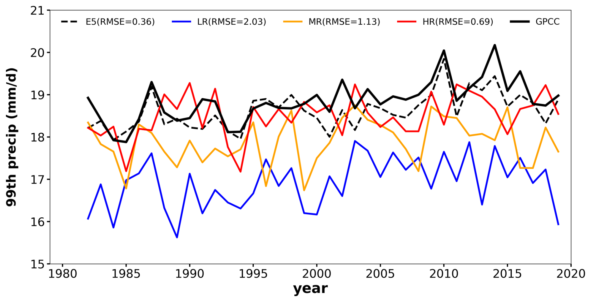
Figure 1 Annual time series of the 99th percentile precipitation using observations (GPCC, black solid line), reanalysis (ERA5, black dash line), and model simulations (LR: blue, MR: orange, HR: red) during 1982–2019 over Europe. RMSE values of 99th percentile precipitation are computed with reference to GPCC values, which are shown within the parentheses (unit: mm d⁻¹).

3 Results

3.1 Extreme precipitation over Europe

We show the time series of 99th percentile precipitation calculated from all grid points and all days in each year over the period 1982–2019 from GPCC, ERA5, and OpenIFS simulations over Europe (Fig. 1). ERA5 simulates an interannual variability of the 99th percentile precipitation similar to that in GPCC. For example, the peak in 2010 and the low in 1994 are well reproduced in ERA5. ERA5 is a reanalysis product that assimilates observations of precipitation; therefore, we expect it to do a better job of reproducing dry (1994) and wet (2010) years than OpenIFS simulations that do not reproduce the same interannual variability as in GPCC or ERA5. However, LR and HR do reproduce the 95 % significant positive trend observed in GPCC (0.03 $\mathrm{mm}{\mathrm{d}}^{-\mathrm{1}}{\mathrm{yr}}^{-\mathrm{1}}$, not shown), which is ∼ 0.02 $\mathrm{mm}{\mathrm{d}}^{-\mathrm{1}}{\mathrm{yr}}^{-\mathrm{1}}$ for both LR and HR, and it is not significant for MR. We note that the OpenIFS simulations use observed SST and sea ice concentrations as boundary conditions, but ozone is taken from a photochemical equilibrium (Cariolle and Teyssèdre, 2007) and aerosol concentrations are taken from Copernicus Atmosphere Monitoring Service (CAMS) monthly climatology. Therefore, we do not expect LR, MR, and HR to reproduce trends driven by ozone or aerosol forcing. We also find that both ERA5 and OpenIFS simulations have relatively lower 99th percentile precipitation rates compared to GPCC (Fig. 1). The RMSE for ERA5 (0.36 mm d⁻¹) is lower than for OpenIFS simulations, which is largest for LR (2.03 mm d⁻¹) and decreases with higher horizontal resolution (i.e., 1.13 mm d⁻¹ for MR and 0.69 mm d⁻¹ for HR). Note that Fig. 1 does not contain any spatial information and that a mismatch between model data and observations can be due to the 99th percentile occurring in different regions and/or with different magnitudes. The RMSE analysis suggests that ERA5 and HR are close to GPCC and LR is far from GPCC.

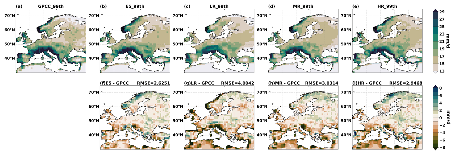
Figure 2 The 99th percentile precipitation over Europe during 1982–2019 from (a) GPCC observations, (b) ERA5 reanalysis, (c) LR, (d) MR, and (e) HR, as well as the corresponding biases and RMSEs in (f) ERA5, (g) LR, (h) MR, and (i) HR.

Figure 2a–e show the spatial distribution of the 99th percentile precipitation over Europe for all days in each season for all years in GPCC, ERA5, and OpenIFS simulations, respectively. In general, the extreme precipitation is very low (∼ 2 mm d⁻¹) in northern Africa, which is to be expected since the mean precipitation is only 0.5 mm d⁻¹ in those regions (Fig. S1 in the Supplement). The extreme precipitation exceeds 30 mm d⁻¹ over mountain areas (e.g., Scandinavian mountains, Alps, and Iberian Peninsula) and the north coast of the Mediterranean but is otherwise lower (∼ 15 mm d⁻¹). The spatial distribution of extreme precipitation matches that of the mean precipitation pattern (Fig. S1). The high 99th percentile precipitation near mountains is likely due to the forced ascent of westerly (Scandinavia, Iberian Peninsula, British Isles) and southerly (Alps) winds. The high 99th percentile precipitation in the north of the Mediterranean is likely because of warm and moist southerly winds from the Mediterranean Sea. The ERA5 and OpenIFS simulations overall reproduce the spatial distribution of the 99th percentile precipitation from GPCC. However, the magnitudes are different, particularly over the Scandinavian mountains, the Alps, and central Europe near 50° N (Fig. 2a–e). Figure 2f–i show the regional biases for the 99th percentile precipitation referenced to GPCC. LR mostly underestimates the 99th percentile precipitation in mountainous areas and deserts by more than 25 % (Fig. 2g), and the biases are reduced when horizontal resolution is increased in MR and HR (Fig. 2h and i). We also notice that LR underestimates the 99th percentile precipitation south of the Alps but overestimates it to the north (Fig. 2g), whereas this bias is negligible in higher-resolution simulations (Fig. 2h and i). This is due to the lower and gentler Alps region simulated in LR (Fig. S2 in the Supplement), where the moist southerly winds do not ascend high enough; therefore, there is less precipitation formed on the southern side and more moisture is advected over the mountains. The moist air descends more slowly over the gentler leeward side in LR than MR (HR); thus, the leeward region may get more precipitation. The reduced biases near mountain regions in the higher-resolution simulations are likely because higher resolution has a better representation of topography and vertical velocity. A cross section of the topography and annual mean vertical velocity at 850 hPa and 62° N (Fig. S3a and b in the Supplement) highlight that the higher-resolution simulations resolve steeper topography, which leads to more ascent and thus more precipitation.

The 99th percentile precipitation over the Alps is more realistic with higher horizontal resolution compared to lower resolution. However, all simulations and ERA5 exhibit a negative bias over northeastern Italy and western Slovenia (Fig. 2f–i). By analyzing the ENSEMBLES daily gridded observational dataset (EOBS) data, we find a similar negative bias as in GPCC but a positive bias in GPCP (Fig. S4d–k in the Supplement). We notice that the extreme precipitation over the Alps (including Slovenia) in GPCP is lower than GPCC and EOBS (Fig. S4a–c), which is likely due to the different data sources and grid methods in different observation datasets (e.g., GPCC and EOBS are gauge-based gridded data on land, but GPCP data combine microwave and infrared measurements, satellites, and rain gauges). We do not know which observation dataset is more realistic; therefore, the cause of the negative bias near Slovenia could be a bias in GPCC or a persistent model bias in the ECMWF-IFS on which both ERA5 and OpenIFS are based. In general, ERA5 has a lower RMSE (2.6 mm d⁻¹) for extreme total precipitation than OpenIFS simulations; i.e., ERA5 has overall lower biases than LR (4.0 mm d⁻¹) and is similar to MR (3.0 mm d⁻¹) and HR (2.9 mm d⁻¹).

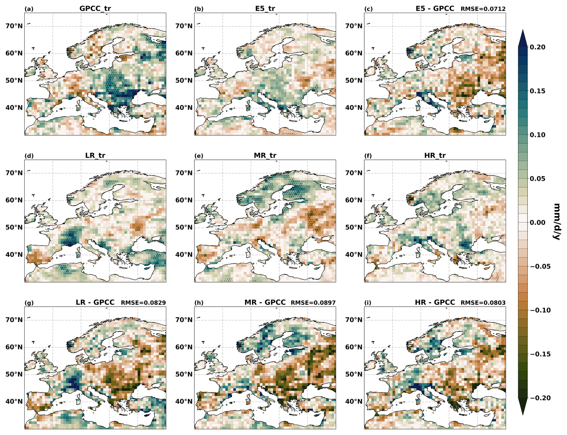
Figure 3 The linear trends of annual 99th percentile precipitation over Europe during 1982–2019 from (a) GPCC observations, (b) ERA5 reanalysis, (d) LR, (e) MR, and (f) HR, as well as the corresponding biases and RMSEs in (c) ERA5, (g) LR, (h) MR, and (i) HR. The shading shows trends at 95 % significance levels.

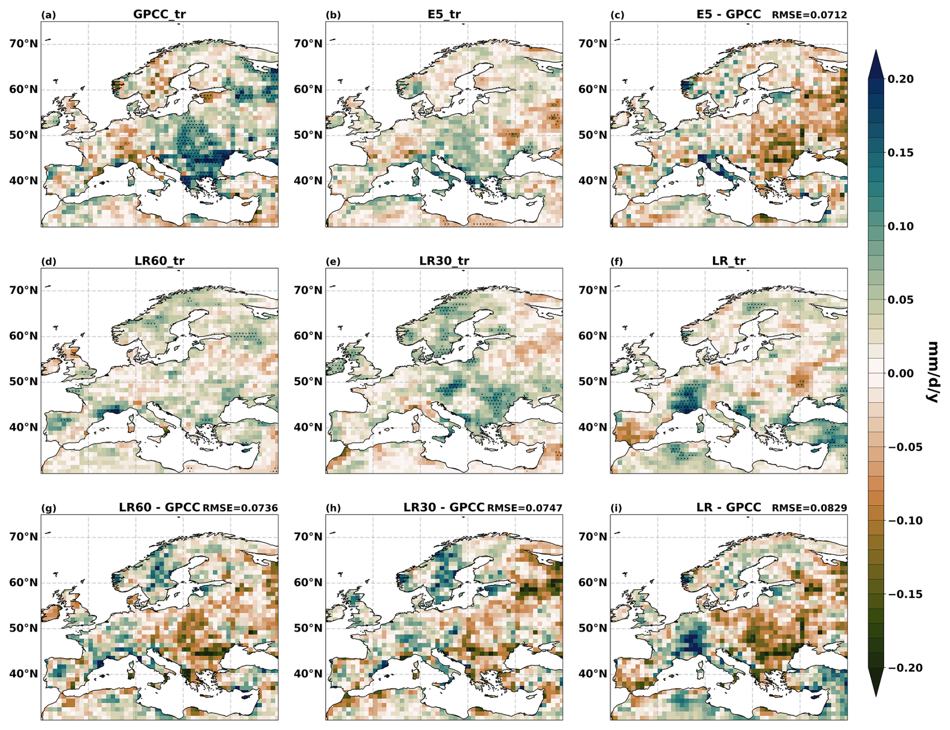
Figure 4 The linear trends of annual 99th percentile precipitation over Europe during 1982–2019 from (a) GPCC observations, (b) ERA5 reanalysis, (d) LR60m, (e) LR30m, and (f) LR, as well as the corresponding biases and RMSEs in (c) ERA5, (g) LR60m, (h) LR30m, and (i) LR. The shading shows trends at 95 % significance levels.

We next calculate the trend for the annual 99th percentile precipitation over Europe (Figs. 3 and 4) and find that the 99th percentile precipitation has a large positive trend in central Europe and a negative trend to the north of the Alps in GPCC (Fig. 3a). ERA5 reproduces the pattern of the trend found in GPCC but is not significant. However, OpenIFS simulations do not have consistent patterns with GPCC (Figs. 3d–f and  4d–f), with only LR30m reproducing the large positive trend in central Europe (Fig. 4d). Overall, the trend is largely underestimated over central Europe but overestimated over northern Europe in OpenIFS simulations. We have not found any consistent improvement across the horizontal resolution and model time step.

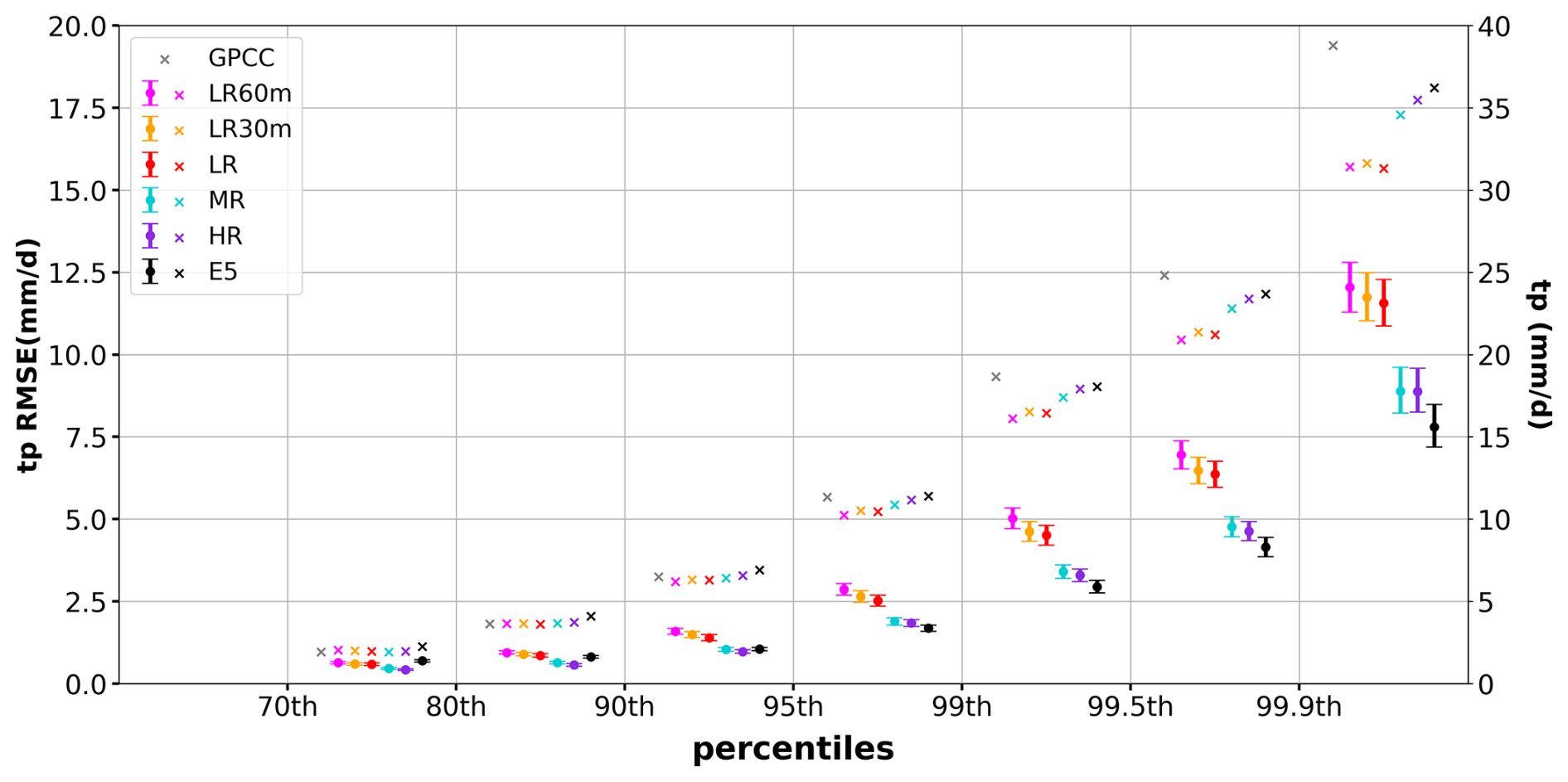
Figure 5 European averaged precipitation amounts and RMSEs (referenced to GPCC) for European total precipitation at different percentile ranges (70th–80th, 80th–90th, 90th–95th, 95th–99th, 99th–99.5th, 99.5th–99.9th, and > 99.9th percentile) in ERA5 (black) and OpenIFS simulations (LR60m: magenta, LR30m: orange, LR: red, MR: blue, HR: purple) during 1982–2019. Cross marks are the precipitation amounts. Dots are the RMSE values, and error bars are the 95 % CI.

In addition to the 99th percentile precipitation and the trend, we calculate annual total precipitation in different percentile ranges, such as 70th–80th, 80th–90th, 90th–95th, 95th–99th, 99th–99.5th, 99.5th–99.9th and larger than 99.9th (i.e., > 99.9th). The RMSEs for ERA5 and OpenIFS simulations referenced to GPCC in each range are shown in Fig. 5. The RMSEs increase exponentially with increasing percentiles, from less than 1 mm d⁻¹ at the 70th–80th percentile range to ∼ 8 mm d⁻¹ above the 99.9th percentile range. The largest RMSE is found for LR60m above the 99.9th percentile range, which is around 12 mm d⁻¹ (CI: 11.3–12.8 mm d⁻¹). We also find that the RMSEs decrease with finer horizontal resolution for all percentile ranges. The CIs of the RMSEs from LR do not overlap with those from higher horizontal resolutions for any percentile range; i.e., the biases from LR are significantly different from those at higher resolutions and thus clearly sensitive to the horizontal resolution. Notably, the RMSE differences between LR simulation and the higher-resolution simulations as well as ERA5 are larger at higher percentile ranges (> 95th) than those at lower percentile ranges (< 95th). This suggests that the extreme precipitation is more sensitive to horizontal resolution than precipitation at lower percentile ranges (< 95th). ERA5 has the smallest RMSE of all datasets above the 95th percentile ranges; i.e., ERA5 has a better representation of the extreme precipitation than our OpenIFS simulations (Fig. 5).

The RMSEs for LR60m, LR30m, and LR are smaller when the model time step is shorter. However, the CI of RMSE overlaps at all percentile ranges; i.e., the sensitivity of precipitation to the model time step is not statistically significant in the low-resolution configurations. While the model time step may influence precipitation, especially convective precipitation, errors from poorly resolved topography probably have a large impact on the RMSE, which would explain the lack of sensitivity to the model time step.

The above analysis is based on the RMSE values, which measure the absolute magnitude of biases. The exponential increase in RMSE with higher percentiles is due to the corresponding exponential increase in precipitation amounts across those percentiles. The relative biases are further explored by calculating the relative RMSE (RRMSE) (Fig. S5 in the Supplement). For the precipitation above the 90th percentile (> 6 mm d⁻¹), RRMSEs are larger at higher percentiles (> 99.9th percentile) than lower percentiles (90th–95th percentile). A larger sensitivity to horizontal resolution at higher percentiles can be also seen, since the RRMSE differences between LR and MR (HR) slightly increase from 5.5 % at the 90th–95th to 6.9 % above the 99.9th percentile. The above RRMSE results are qualitatively consistent with the larger RMSE and sensitivity to horizontal resolution at higher percentiles shown in Fig. 5, but quantitatively RRMSE shows smaller variations across percentiles than RMSE does. However, the RRMSEs at the 70th–90th percentile ranges show comparable magnitude and sensitivity to those above the 99th percentile, which is related to the very low precipitation amounts at these percentiles (1.9 mm d⁻¹ for 70th–80th and 3.6 mm d⁻¹ for 80th–90th percentile range).

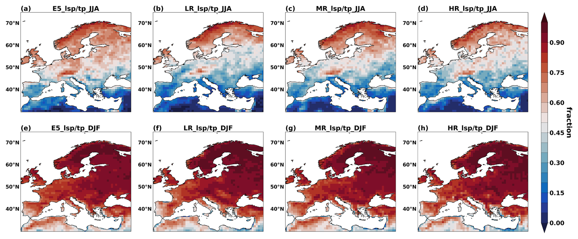
Figure 6 Contribution of large-scale precipitation to extreme precipitation (> 99th percentile) in ERA5 (a, e), LR (b, f), MR (c, g), and HR (d, h) over Europe in JJA (a–d) and DJF (e–h) over the period 1982–2019.

3.2 Relative roles of convective and large-scale precipitation

Total precipitation is the sum of convective and large-scale precipitation. Convective precipitation is related to unresolved convective motions. It comes from physical processes whose scales are smaller than the resolution of the model and therefore need to be parameterized. On the other hand, large-scale precipitation is related to large-scale processes larger than the model resolution that can be resolved. When moving to higher horizontal resolutions, large-scale precipitation is likely to increase, and the ratio between convective and large-scale precipitation may change. In this section we split the extreme precipitation into convective and large-scale precipitation to see their sensitivities to horizontal resolution and model time step. The extreme precipitation is nearly 100 % large-scale precipitation over northern Europe, more than 90 % over central Europe, and more than 70 % over western and southern Europe in DJF (Fig. 6e–h). However, in JJA the extreme precipitation is mostly large-scale precipitation over northern Europe (> 70 %) and convective precipitation in the Mediterranean region (> 70 %) (Fig. 6a–d). Due to the seasonally dependent large-scale precipitation contribution to extreme total precipitation, we discuss convective and large-scale precipitation sensitivities to horizontal resolution and time step in JJA and DJF separately. The ratios between convective and large-scale precipitation are also discussed here. Considering that the ratios over parts of Mediterranean region are very large, which influence the results a lot, we remove that region and only include the region north of 40° N (i.e., 40–72° N, 10° W–40° E) in this section.

Table 1 The experiment details with different horizontal resolutions and model time steps in OpenIFS.

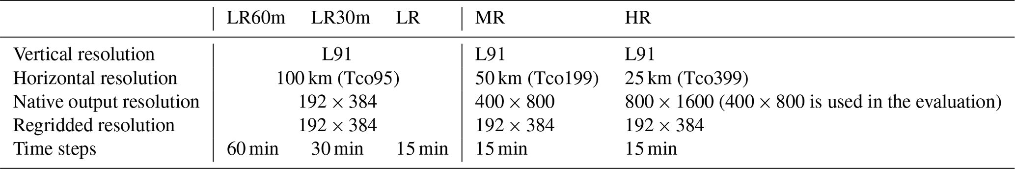
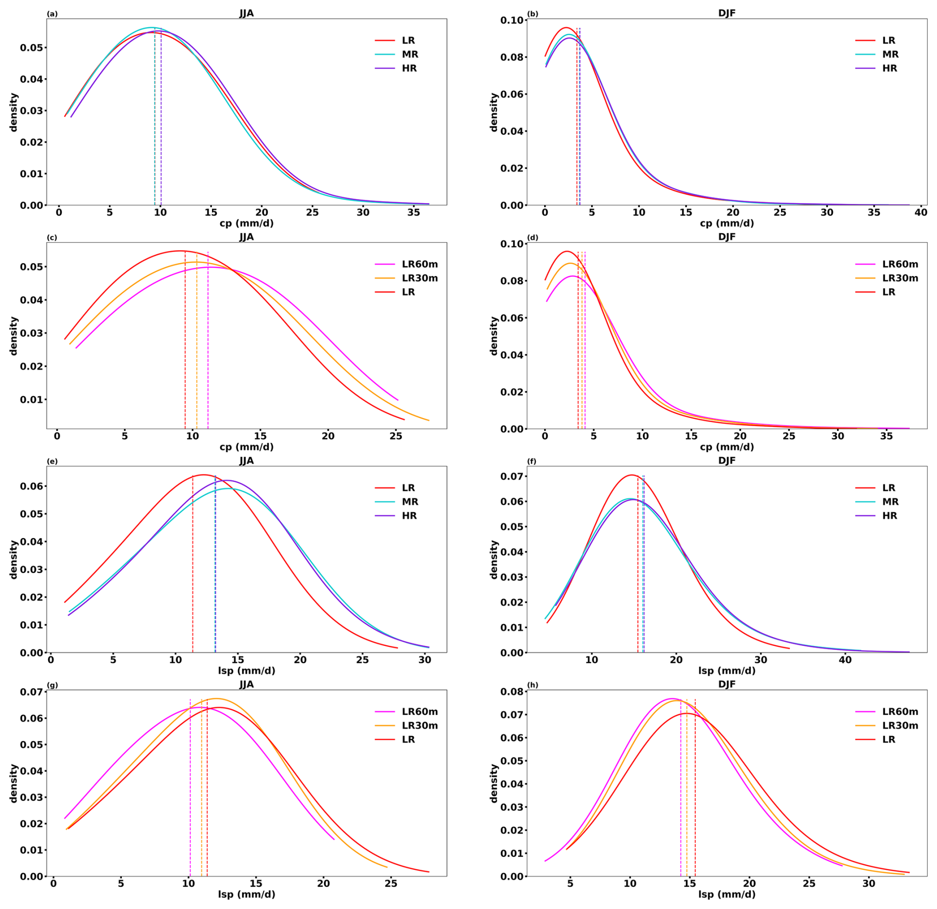
Figure 7 European convective (a–d) and large-scale precipitation (e–h) distribution across different horizontal resolutions (a, b, e, f) and model time steps (c, d, g, h) during extreme precipitation days in JJA and DJF (LR60m: magenta, LR30m: orange, LR: red, MR: blue, HR: purple). The time period is 1982–2019. The dashed lines are the mean values of each distribution.

During the extreme precipitation days, Europe has more convective precipitation in JJA (∼ 10 mm d⁻¹) than in DJF (∼ 3.7 mm d⁻¹), and their distributions do not change much across horizontal resolution (Fig. 7a and b), while from the significance test (Table 2a), we found that JJA convective precipitation only increases significantly moving from MR to HR, and DJF convective precipitation significantly increases from LR to MR (HR). However, the convective precipitation distributions vary noticeably across model time steps, as shown in Fig. 7c and d. As the model time step is reduced, the distributions of JJA convective precipitation move to the left; thus, less convective precipitation is simulated in shorter-time-step simulations. DJF has similar results as in JJA. The changes are significant (Table 2a) – that is, convective precipitation in OpenIFS is sensitive to model time step.

Table 2 The p values of t tests for convective precipitation (a), large-scale precipitation (b), and their ratio (c) distribution across horizontal resolutions and model time steps. The bold means the result is significant (p value < 0.05).

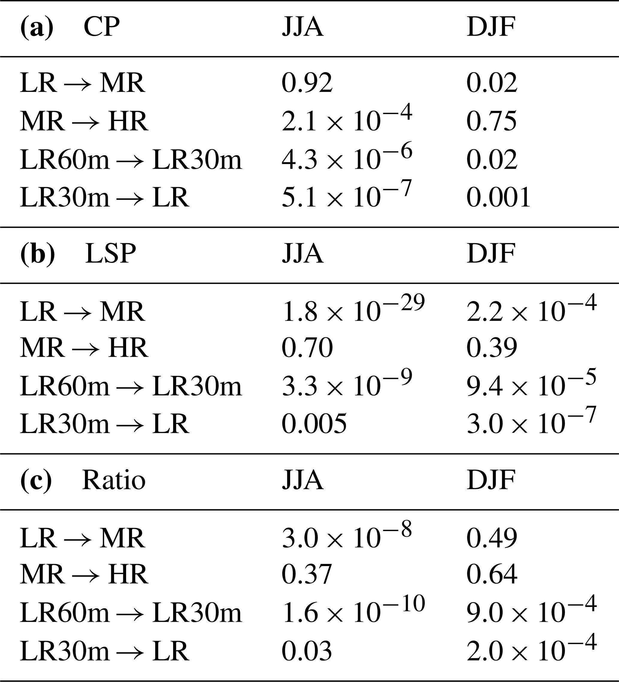
The distributions of large-scale precipitation in MR and HR (Fig. 7e) shift to the right compared to LR in JJA, and MR and HR have significantly more large-scale precipitation (13.2 mm d⁻¹) than LR (11.4 mm d⁻¹). In DJF, the distribution peaks of LR, MR, and HR are similar (Fig. 7f), but MR and HR have bigger tails than LR. Thus, MR and HR have more large-scale precipitation than LR. The increase in large-scale precipitation is likely due to the better-simulated topography at higher horizontal resolution, where more large-scale precipitation is resolved. The changes in large-scale precipitation in both JJA and DJF from LR to MR are significant, but not from MR to HR (Table 2b). This means that the large-scale precipitation is sensitive when horizontal resolution is increased from LR to MR, but not from MR to HR. Large-scale precipitation also significantly increases when the model time step is shortened from 60 to 30 min and also from 30 to 15 min in both JJA (Fig. 7g) and DJF (Fig. 7h) – that is, large-scale precipitation is also sensitive to the model time step.

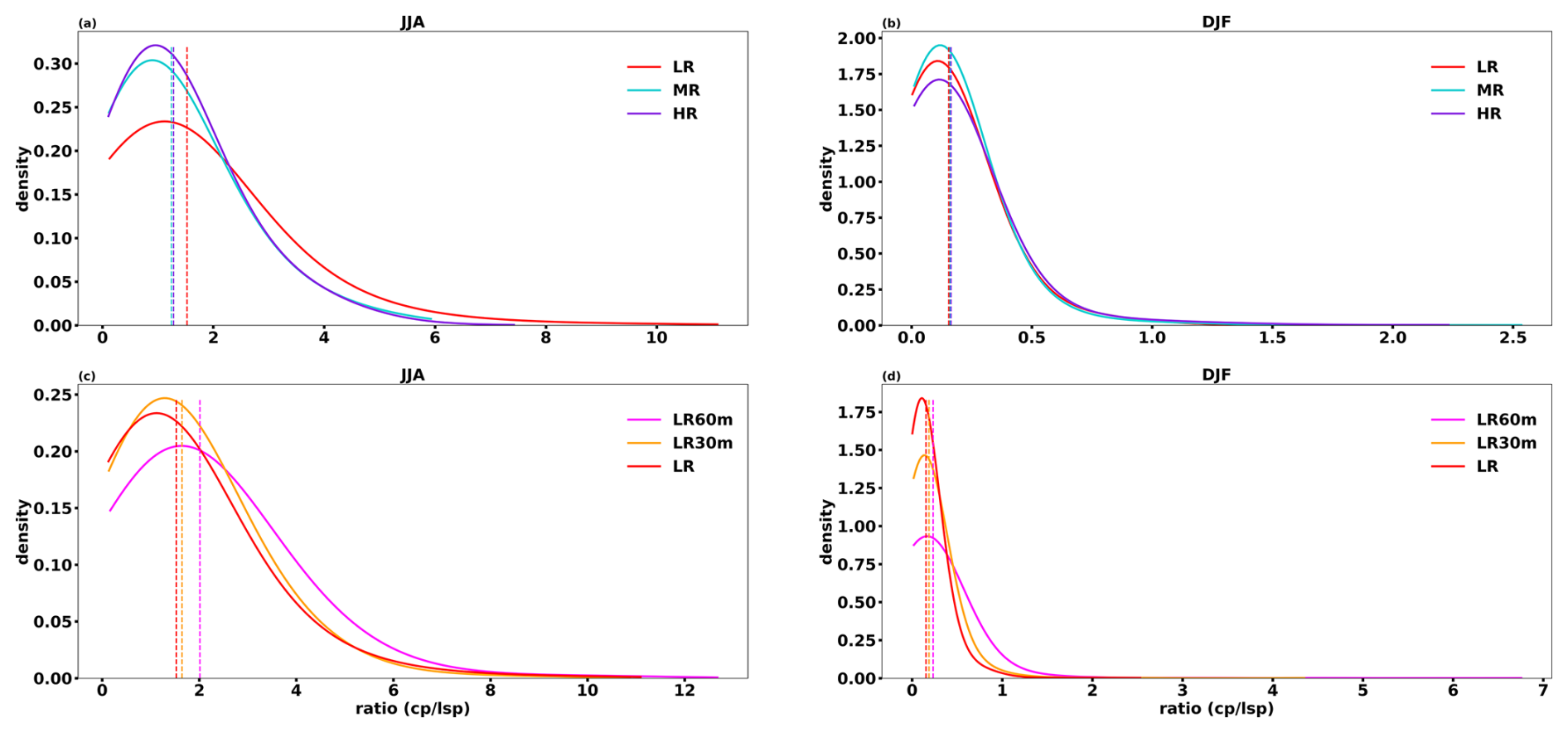
Figure 8 The ratio between European convective and large-scale precipitation during extreme precipitation days across different horizontal resolutions (a, b) and model time steps (c, d) in JJA and DJF (LR60m: magenta, LR30m: orange, LR: red, MR: blue, HR: purple). The dashed lines are the mean values of each distribution.

We further analyze the distribution of the ratio between convective and large-scale precipitation in JJA and DJF, shown in Fig. 8. For different resolutions, the ratio distributions from MR and HR are narrower and slightly shift to the left compared to LR in JJA (Fig. 8a), which means MR and HR have smaller mean ratios (1.5) than LR (∼ 1.25). That is due to the large-scale precipitation increasing by 16 % with finer horizontal resolution, whereas convective precipitation only increases by 6 %. However, the ratios between convective and large-scale precipitation do not vary significantly with higher horizontal resolutions in DJF (Fig. 8b). When moving to a shorter model time step, the ratios significantly decrease in JJA (from 2 to 1.5) and DJF (Fig. 8c and d, Table 2c). It is related to the significant decreasing convective and increasing large-scale precipitation with a shorter model time step.

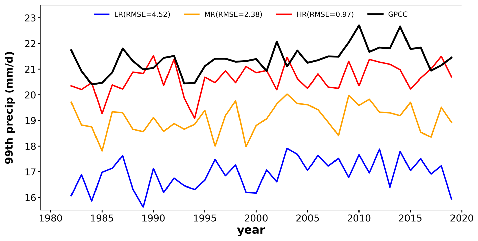
Figure 9 Annual time series of the 99th percentile precipitation using observations (GPCC, black solid line) and model simulations at their native resolution (LR: blue, MR: orange, HR: red) during 1982–2019 over Europe. RMSE values of 99th percentile precipitation are computed with reference to GPCC, which are shown within the parentheses (unit: mm d⁻¹).

In summary, during extreme precipitation days, large-scale precipitation increases with higher horizontal resolution and a shorter model time step; however, convective precipitation increases with higher horizontal resolution and decrease with a shorter model time step. Convective precipitation is more sensitive to model time steps than to horizontal resolutions, while large-scale precipitation is sensitive to both. Therefore, the extreme precipitation sensitivity to horizontal resolution is mostly from large-scale precipitation.

We also analyze the mean state convective and large-scale precipitation sensitivity to horizontal resolution and model time step (Figs. S6 and S7 in the Supplement). Convective precipitation decreases and large-scale precipitation increases with higher horizontal resolution and a shorter model time step; therefore, their ratio decreases. Their sensitivities to resolutions and time steps are less significant in the mean state than in the extreme state, especially for mean convective precipitation, which is only significantly sensitive when shortening the model time step from 30 to 15 min. The changes in mean convective precipitation with horizontal resolution are opposite with the extreme one (Figs. S6a, b and 7a, b), but these changes for both extreme and mean states are very small, and convective precipitation is more sensitive to model time steps in both states (Figs. S6c, d and 7c, d).

4 Discussion and conclusion

We have investigated the sensitivity of extreme precipitation across different horizontal resolutions and model time steps in atmosphere-only experiments with the OpenIFS. Comparing extreme precipitation (defined as total daily precipitation at the 99th percentile) from OpenIFS simulations, reanalysis (ERA5), and observations (GPCC), we find that MR and HR mostly better represent the precipitation extremes compared to LR. We also found a more significant sensitivity to the horizontal resolution for precipitation above the 95th percentile and less sensitivity for lower percentile ranges (< 95th) (Fig. 5). These OpenIFS-based results are similar to Kopparla et al. (2013), who found that the bias of extreme precipitation in the high-resolution simulation (25 km) was reduced compared to the lower-resolution simulations (100 and 200 km) over Europe in their atmospheric model, but not for precipitation at lower percentiles (i.e., < 95th). However, the sensitivity to the horizontal resolution found by Kopparla et al. (2013) was not significant over Europe, which is rather different from our results as we have found a significant difference across the horizontal resolutions. In contrast to the extreme precipitation, the bias for global mean precipitation does not decrease much with higher horizontal resolution in OpenIFS. Similar results are also found in other AGCMs (e.g., ECHAM6, OpenIFS, HadGEM1, and HadGEM3) (Hertwig et al., 2015; Savita et al., 2024; Schiemann et al., 2014; Demory et al., 2020). However, Delworth et al. (2012) found an improvement in the global mean precipitation with higher horizontal resolution in a coupled model (GFDL).

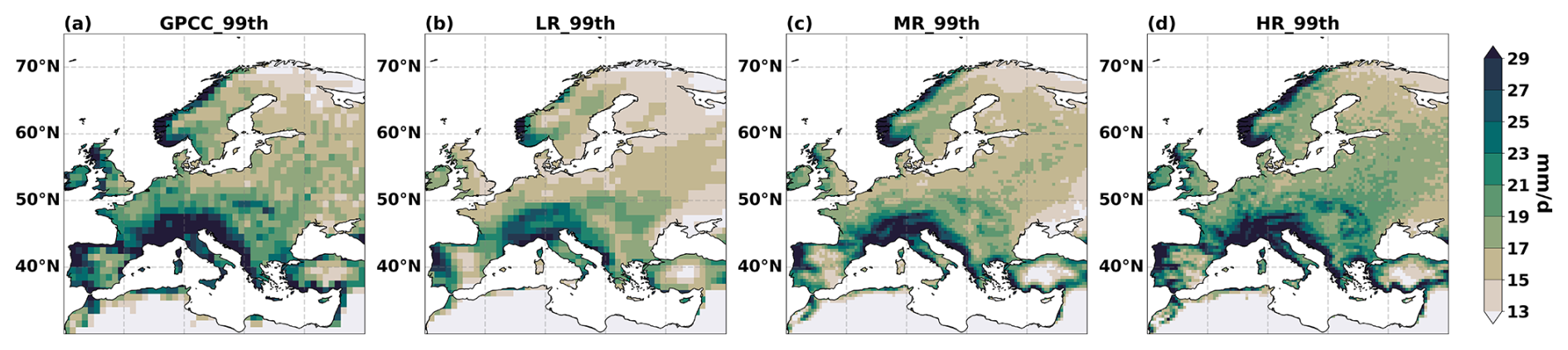
Figure 10 The 99th percentile precipitation over Europe during 1982–2019 from (a) GPCC observations, (b) LR, (c) MR, and (d) HR at their native resolution.

The improvements due to higher horizontal resolution for the extreme precipitation are mostly over the mountain areas, consistent with previous studies which found the effect of horizontal resolution to be the largest in areas with complex topography over Europe and also other regions for mean and extreme precipitation (Demory et al., 2020; Iles et al., 2020; Monerie et al., 2020; Prein et al., 2013; Torma et al., 2015). The sensitivity to the horizontal resolution comes from the large-scale precipitation, which is likely because of the better-resolved topography. However, the convective precipitation is more sensitive to the model time step than it is to the horizontal resolution.

In our results, larger improvements are obtained when the horizontal resolution is increased from LR to MR, but relatively smaller improvements are found from MR to HR. This diminishing return is also found by Roberts et al. (2018) from ∼ 50 to ∼ 25 km in ECMWF-IFS, but for climatological surface biases. The simulation of extratropical cyclones, tropospheric circulation, and tropical mean precipitation in ECMWF-IFS also has smaller improvements from 39 to 16 km than from 126 to 39 km (Jung et al., 2012). However, the tropical cyclone intensity and intense storm structure, which often cause extreme precipitation in the tropics (Gori et al., 2022; Zhu and Quiring, 2022), are adequately simulated at 16 km, but not at 126 and 39 km resolutions in ECMWF-IFS (Manganello et al., 2012). Therefore, the diminishing return in this study is valid for European extreme precipitation but may not be for tropical extreme precipitation.

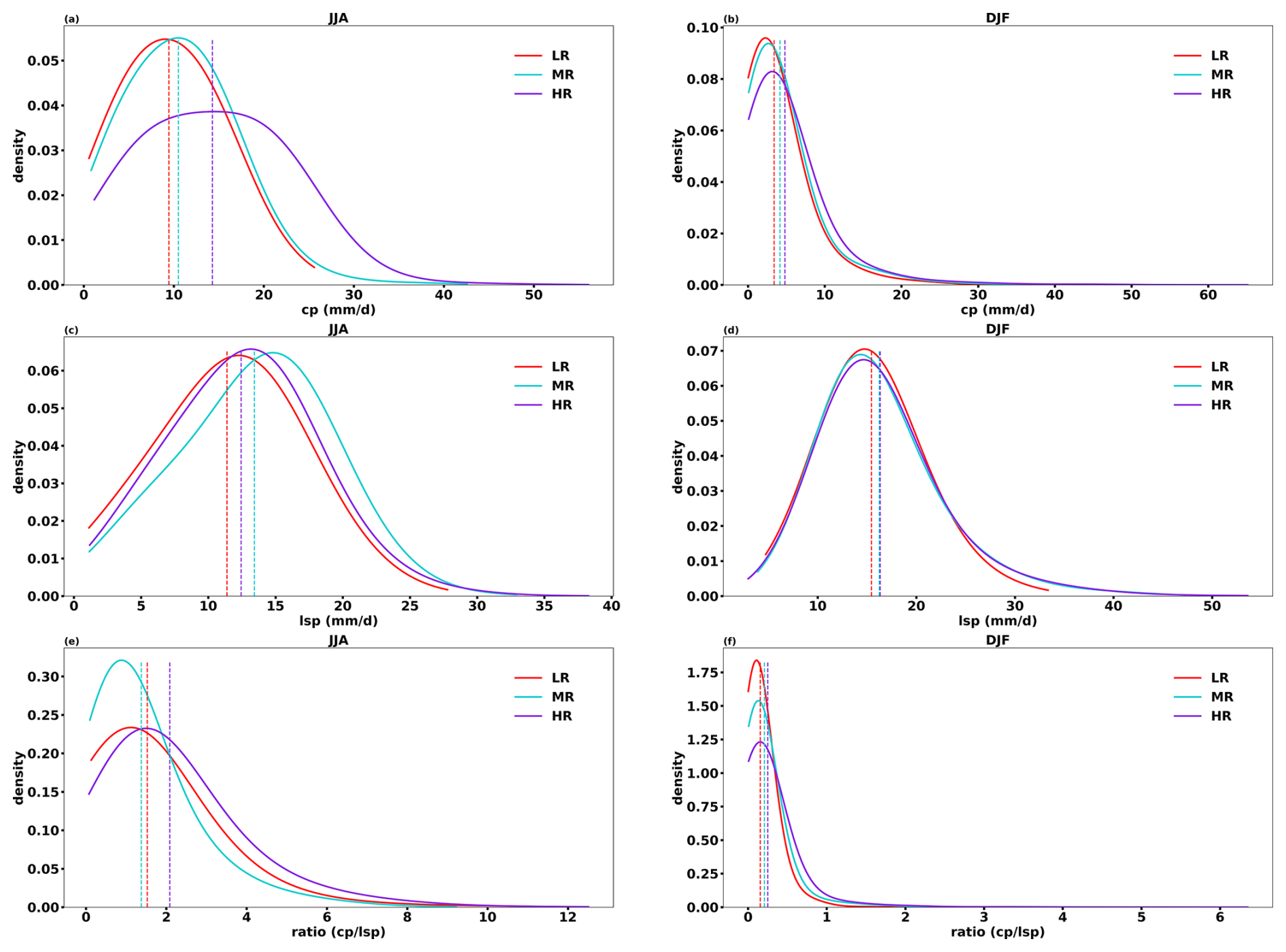
Figure 11 European convective precipitation (a, b) and large-scale precipitation (c, d) distribution and ratio ($\mathrm{CP}/\mathrm{LSP}$) at their native resolution across different horizontal resolutions during extreme precipitation days in JJA and DJF (LR: red, MR: blue, HR: purple). The time period is 1982–2019. The dashed lines are the mean values of each distribution.

Since the analysis of horizontal resolution's impact is based on regridded data, it may therefore be influenced by the regridding process. The native resolution of our model output is 192 × 384 for LR, 400 × 800 for MR, and 800 × 1600 for HR; however, only 400 × 800 for HR output is saved due to computational cost. Similar to the result of regridded data (Fig. 1), extreme precipitation at the native resolution is underestimated in OpenIFS compared to GPCC, and the biases decrease with higher horizontal resolution (Fig. 9). Extreme precipitation at native resolutions also has a similar spatial distribution as that at regridded resolution (Figs. 10 and 2), such as more extreme precipitation in mountain areas. However, the extreme precipitation is larger (13 % for GPCC, 7 % for MR, and 12 % HR) at the native resolution than at regridded resolution because some extreme precipitation is smoothed when regridding to 0.9° × 0.9°. The RMSEs of extreme precipitation against GPCC are also larger at the native resolution (Fig. 9) than at the regridded resolution (Fig. 1), which holds across different percentiles (Fig. S8 in the Supplement). Moreover, the sensitivity of extreme precipitation to horizontal resolution is also greater at the native resolution (Fig. S8). Convective and large-scale precipitation during extreme precipitation days increases with higher horizontal resolution (Fig. 11a–d), consistent with regridded results. The convective-to-large-scale precipitation ratio significantly decreases from LR to MR in JJA (Fig. 11e), which is also consistent with regridded results. However, the ratio increases from MR to HR in JJA at the native resolution, differing from regridded analysis, likely due to the dramatically increasing convective precipitation from MR to HR in JJA. Overall, regridding the model dataset does not change the conclusion qualitatively in this study but causes quantitative differences.

Moreover, the choice of observation dataset is a key factor for assessing the impact of the horizontal resolution and model time step on extreme precipitation. Most observation precipitation data are from one of three categories: gauge-based products, satellite products, and merged satellite–gauge products. Since the satellite products are constructed with satellite microwave and/or infrared measurements, with/without gauged-adjusted estimates, differences exist between these products. Besides, the gauge-based products are highly dependent on the choice of stations and interpolation schemes. It is hard to say which product is closer to reality, as different regions may have different observation datasets that best suit the analysis. In particular, we note that not all products are suitable for extreme analysis. For example, GPCP's main scope is to construct a reliable climate data record, and it has been developed with a priority of ensuring the long-term stability of data (Adler et al., 2017). Masunaga et al. (2019) found that the frequency of GPCP daily precipitation quickly drops below all other datasets once the precipitation exceeds 30 mm d⁻¹. Also, the time series of GPCP extreme precipitation over the ocean exhibits a jump to lower 99th percentiles in late 2008/early 2009, which is not present in all other datasets, coinciding with the change in utilization of the Special Sensor Microwave/Imager (SSM/I) and Special Sensor Microwave Imager Sounder (SSMIS). The lower 99th percentile precipitation suggests that the GPCP dataset might not be applied to extreme analysis (Masunaga et al., 2019). Therefore, we only use GPCC observation data as the reference to explore the model performance. In Fig. 2f–i the 99th percentile precipitation is largely underestimated in the eastern Alps region by ERA5 and all model simulations. The biases are insensitive to horizontal resolution. It is likely a persistent model bias in ECMWF-IFS or a bias in GPCC. Comparing model output to multiple observational precipitation products instead of relying on a single one may be a good way to reduce these biases. Multiple observational products can be taken as an ensemble, which provide a spread of observational estimates and allow insights into whether and which model configurations sit within this observational spread.