Representing lateral groundwater flow from land to river in Earth system models

Lateral groundwater flow (LGF) is an important hydrologic process in controlling water table dynamics. Due to the relatively coarse spatial resolutions of land surface models, the representation of this process is often overlooked or overly simplified. In this study, we developed a hillslope-based lateral groundwater flow model. Specifically, we first developed a hillslope definition model based on an existing watershed delineation model to represent the subgrid spatial variability in topography. Building upon this hillslope definition, we then developed a physical-based lateral groundwater flow using Darcy’s equation. This model explicitly considers the relationships between the groundwater table along the hillslope and the river water table levels. We coupled this intra-grid model to the land component (E3SM Land Model: ELM) and river component (MOdel for Scale Adaptive River Transport: MOSART) of the Energy Exascale Earth System Model (E3SM). We tested both the hillslope definition model and the lateral groundwater flow model and performed sensitivity experiments using different configurations. Simulations for a single grid cell at 0.5°×0.5° within the Amazon basin show that the definition of hillslope is the key to modeling lateral flow processes and the runoff partition between surface and subsurface can be dramatically changed using the hillslope approach. Although our method provides a pathway to improve the lateral flow process, future improvements are needed to better capture the subgrid structure to account for the spatial variability in hillslopes within the simulated grid of land surface models.

1 Introduction

Lateral groundwater flow (LGF) is an important hydrologic process in the water cycle. It not only redistributes groundwater resources across the landscapes but also influences the groundwater and stream water (GW–SW) interactions (Miguez‐Macho and Fan, 2012). However, in large-scale Earth system models (ESMs), LGF is often estimated using empirical methods that do not consider changes in land surface heterogeneity, which is considered one of the three grand challenges in land surface modeling (Oleson et al., 2013; Fisher and Koven, 2020). Consequently, substantial uncertainty persists in these estimates of hydrological and energy state variables and fluxes.

Although subsurface groundwater flow is often considered relatively slow compared to overland surface runoff, its total contribution to streamflow can be significant. Many studies found that subsurface flow dominates streamflow contribution in many environments, especially when precipitation is limited (Miller et al., 2016; Xie et al., 2024). Others also reported that its contribution varies with seasons, and even during the wet season, its contribution can reach up to 40 % (Mortatti et al., 1997). Besides, GW–SW interactions are active throughout the year and are influenced by both land and river conditions (Markstrom et al., 2008).

Traditionally, lateral groundwater flow, including GW–SW interactions, is often modeled at a regional scale using high-spatial-resolution (e.g., 10 m–1 km) groundwater flow models. These models often simulate the cell-to-cell or between-cell lateral groundwater flow by solving three-dimensional (3D) partial differential equations implicitly based on hydraulic head differences (Langevin et al., 2017; Liao and Zhuang, 2017; Fang et al., 2022). In unconfined aquifers, the hydraulic head closely aligns with the water table, often influenced by the surrounding surface topography. Specifically, the water table often follows the surface topography, and groundwater flows from the upland to the alluvial fan before entering the river channels or large waterbodies. Besides the 3D modeling approach, regional hydrologic models also use the two-dimensional (2D) approach to simulate the LGF along hillslopes, as many studies recognized its impacts on the belowground water table and soil moisture along the hillslope (Troch et al., 2003; Marcais et al., 2017; Zhang et al., 2024). In this case, an array of connected columns often represents an idealized hillslope, and the nonlinear hillslope-storage Boussinesq (HSB) equation is often used to simulate the hydrologic processes considering the distributions of soil and vegetation in different columns.

Meanwhile, in large-scale ESMs and land surface models (LSMs), because the horizontal spatial resolutions (10–200 km) are much coarser than the vertical spatial resolution (∼100 m) (Brunke et al., 2016), these models generally do not simulate the between-cell groundwater flow (Qiu et al., 2024). Moreover, these models cannot simulate the within-cell lateral groundwater flow using the hydraulic head gradient within each grid cell because their geospatially unaware subgrid structures do not support the hydraulic gradient calculation. Instead, some LSMs use empirical functions to estimate the within-cell or intra-grid LGF as a function of water table depth (WTD) and surface topography (Oleson et al., 2013).

Incorporating the 3D or 2D regional-scale approach into large-scale ESMs presents persistent challenges due to several factors. First, the global-scale high-resolution (∼1 km) 3D approach is nearly unachievable due to its computation demand. It was not until recently that the utilization of the supercomputers or graphics processing unit (GPU) made this approach feasible. For example, recent studies made processes using advanced high-performance computing techniques to run large-scale 3D groundwater flow models at 1 km spatial resolution (Hokkanen et al., 2021). Alternatively, some studies proposed a hybrid approach that only uses the 3D approach at the subgrid level while a simplified formula is used at the cell interface (Wang et al., 2020). This approach, however, does not consider the river networks. Several studies also attempted to use an explicit instead of implicit 3D approach to reduce the computational cost in a global-scale groundwater model (Fan et al., 2013). Second, the 2D hillslope approach draws much attention because it can simulate the within-cell LGF without the high computational cost compared with the 3D approach (Swenson et al., 2019; Chaney et al., 2021). However, due to scale differences, there is a significant challenge in transforming a land surface grid cell into a hillslope-based data structure. Traditional hillslope hydrology often focuses on individual idealized hillslopes, i.e., uniform, convergence, and divergence hillslopes (Paniconi et al., 2003). However, an LSM grid cell, regardless of structured or unstructured, is often relatively large and may contain multiple hillslopes at different locations. Besides, each hillslope may be linked to different river channels, main or tributaries (Xu et al., 2022). Lastly, a portion of the grid cell may not even belong to the same watershed. Therefore, applying the hillslope approach to the LSM requires careful consideration of the scale differences (Fig. 1).

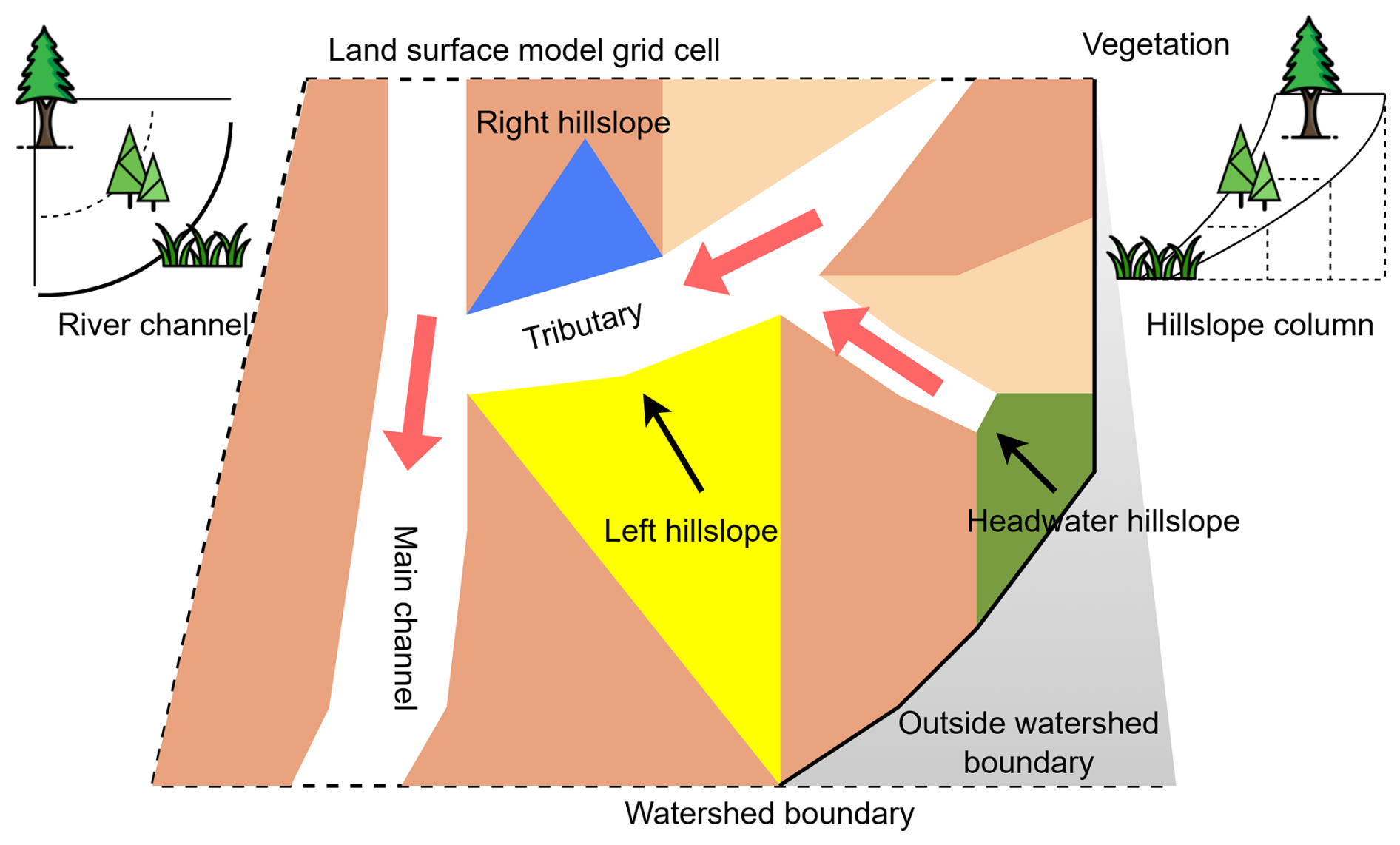
Figure 1 Illustration of the land surface with river channels and hillslopes within a land surface model (LSM) grid cell. The river channels include the main channel and tributaries. Colored polygons are conceptual hillslope types. The yellow, blue, and green polygons are left, right, and headwater hillslopes, respectively. Red arrows are the flow direction in the channels. Black arrows are the flow direction along the hillslope. The area marked in grey represents the portion that does not belong to this watershed. The upper-left and upper-right mini plots illustrate the left/right (divergent) and headwater (convergent) hillslopes along a river channel or headwater with different vegetation distributions. Sizes are not drawn to scales.

Most existing LSMs already have a built-in subgrid structure which often defines classes or groups using area fractions (Best et al., 2011; Oleson et al., 2013; Guimberteau et al., 2018). Therefore, any group entity may spread out at different locations (e.g., hillslope) or outside the watershed. For example, a plant functional type (PFT) may occupy 30 % of a grid cell, but the model assumes it is uniformly distributed across the grid cell. However, due to energy and water availability, this PFT may only be distributed at a certain hillslope in reality. Moreover, an LSM grid cell may also contain other hydrologic features, including rivers, lakes, and wetlands. All of these hydrologic features may interact with the land surface differently. For example, a flooding event may occur at the main river channel but is absent near the tributaries (Xu et al., 2022). Taken together, representing the land surface using the hillslope subgrid structure poses a great challenge. To address this challenge, several studies have developed various approaches to represent LSM grid cells using hillslopes with different levels of complexity. For example, some studies use subgrid structure and connectivity from upland to lowland to mimic the hillslope concept (Chaney et al., 2021).

In this study, we developed a new hillslope-based hydrologic model to simulate the within-cell or intra-grid LGF within the land component of the Energy Exascale Earth System Model (E3SM) (Golaz et al., 2022). This hillslope-based hydrologic model within the E3SM Land Model (ELM) (1) uses a simple approach to represent the LSM grid cells with hillslopes, (2) uses Darcy's law to estimate the within-cell LGF along the hillslope, and (3) considers the one-way GW–SW interactions through hillslope–river coupling. We tested different hillslope definition configurations. We investigated the model behaviors by performing simulations using different model configurations. Our analyses of the simulation results show that the representation of the hillslope is the key to modeling lateral flow processes, and our method provides a promising pathway to improve the large-scale hydrological and biogeochemistry modeling using the hillslope-based subgrid structure.

2 Method description

2.1 Current method

E3SM is an Earth system model that includes the atmosphere, ocean, sea ice, river, and land components which are coupled using the Common Infrastructure for Modeling the Earth (CIME) (Golaz et al., 2019, 2022). The E3SM Land Model (ELM) was developed based on the Community Land Model version 4.5 (CLM v4.5) with notable improvements in soil hydrology and biogeochemistry. It simulates major land surface and subsurface biogeochemical and biogeophysical processes, including the hydrologic and carbon cycles (Oleson et al., 2013).

Similar to other LSMs, ELM mainly simulates processes in the vertical direction within each grid cell. To generate streamflow, ELM sends surface and subsurface runoff to the E3SM river component, MOdel for Scale Adaptive River Transport (MOSART), to simulate in-stream processes (Li et al., 2013). In ELM, LGF, simplified as the subsurface runoff, mainly comes from unconfined aquifers. It is modeled using a groundwater drainage function, which considers soil water thermal status (ice/liquid) and WTD (Oleson et al., 2013). This drainage function is expressed as

$$\begin{array}{}\text{(1)}& Q_{\mathrm{drai}}={\mathrm{\Theta }}_{\mathrm{ice}}\times Q_{\mathrm{drai},\max }\times e^{-f_{\mathrm{drai}}\times z_{\mathrm{\nabla }}},\end{array}$$

where Q_drai is the groundwater drainage (mm s⁻¹), Θ_ice is the ice impedance factor (fraction), Q_drai,max is the maximal drainage rate, f_drai is a depth decay factor (m⁻¹), and z_∇ is the WTD (m). The ice impedance factor Θ_ice restricts drainage in fully or partially frozen soils and is calculated as

$$\begin{array}{}\text{(2)}& {\displaystyle }& {\displaystyle }\mathit{\alpha }={\displaystyle \frac{\sum _{i=jwt}^{i=N_{\mathrm{levsoi}}}{F}_{\mathrm{ice}}\mathrm{\Delta }{z}_i}{\sum _{i=jwt}^{i=N_{\mathrm{levsoi}}}\mathrm{\Delta }{z}_i}},\text{(3)}& {\displaystyle }& {\displaystyle }{\mathrm{\Theta }}_{\mathrm{ice}}={\mathrm{10}}^{-\mathrm{\Omega }\times \mathit{\alpha }},\end{array}$$

where Ω is an adjustable parameter, F_ice is the ice fraction in the ith soil layer, Δz_i is the soil layer thickness (mm), jwt is the soil layer index where water table rests, and N_levsoi is the total number of soil layers. The maximal drainage rate Q_drai,max is calculated as

$$\begin{array}{}\text{(4)}& Q_{\mathrm{drai},\max }=\mathrm{10}\sin \left(\mathit{\beta }\right),\end{array}$$

where β is the average grid cell topographic slope (radian) derived from the high-resolution digital elevation model (DEM). The maximal drainage rate occurs when the water table is at the land surface (z_∇=0.0).

Although the current method can provide reasonable estimates in most applications if calibrated parameters are used, its applications can be limited for the following reasons:

1. It does not consider the scenario when the water table is above the land surface (z_∇<0.0). For example, if a portion of the grid cell is inundated near the river channel, the drainage function will underestimate the groundwater flow because it uses the constant maximum drainage rate (Scudeler et al., 2017).

2. It does not consider the aquifer properties, including hydraulic conductivity, that control the groundwater flow rate.

3. It does not explicitly consider the GW–SW interactions (Chaney et al., 2021). In the default method, the LGF is only influenced by the land surface condition, regardless of river conditions. Consequently, it cannot produce a “losing-stream” scenario when the groundwater system receives water from the river during a flooding event.

4. Because this method is based on existing area fraction-based subgrid structure, it omits the spatial connectivity. As a result, it cannot explicitly provide feedback between the water table and soil moisture. For example, this method cannot be used to improve modeling of the groundwater availability and soil moisture at different elevation bands, which are critical for tree mortality during extreme droughts.

2.2 A new hillslope-based method

The ELM hillslope-based lateral groundwater flow model (HLGF) was developed based on several existing hillslope hydrology models with modifications (Maquin et al., 2017; Chaney et al., 2021). Within-cell saturated groundwater lateral flow is modeled using the classical Darcy's equation based on water table gradient and aquifer properties. This model consists of two major components: the conceptual hillslope definition and the corresponding numerical method. Below, we introduce the conceptual hillslope definition and then provide the details of the numerical model.

2.2.1 Hillslope definition model

Rather than categorizing subgrid heterogeneity by attributes, our approach focuses on spatial connectivity. Specifically, we aggregate all elements on the same hillslope into a single computational unit. Therefore, the definition of a hillslope is key to the model's performance. As described in Fig. 1, an LSM grid cell often contains multiple hillslopes at different locations. While most existing LSMs lack a subgrid structure that is capable of resolving individual hillslopes, our study necessitates such granularity. To bridge this gap, we propose aggregating hillslopes into a single representative unit.

In general, hillslopes are often defined by several geometric characteristics: (1) area, (2) length, (3) width, (4) slope, and (5) divergent or convergent angle (Paniconi et al., 2003). However, within an ESM framework, these characteristics may not resemble their physical attributes, especially if aggregation was applied. To define the hillslopes, modelers often have to rely on various terrain analyses, such as the watershed delineation process or geospatial statistics. In this study, we investigated two different approaches to define the hillslopes.

In the first approach, we utilize an existing watershed delineation model (HexWatershed) (Liao et al., 2020) with modifications (Table B1) to define the hillslopes and calculate their geometric characteristics (Liao et al., 2023; Liao, 2022a). This model defines hillslopes in two steps: (1) watershed delineation to define the river networks and (2) hillslope delineation for each stream segment–subbasin pair. Specifically, it tracks where each high-resolution DEM grid cell within this subbasin enters the river channel and groups them into left and right hillslopes (Fig. 2). If a stream segment is a headwater, then all the DEM grid cells entering through the first headwater grid cell are grouped into a headwater hillslope. This definition is illustrated in Fig. 2 and the Supplement (Sect. B1). After all the hillslopes are defined, their geometric characteristics, including area, width, length, and slope, are calculated. We assume the left/right hillslopes are uniform and the headwater hillslopes are convergent.

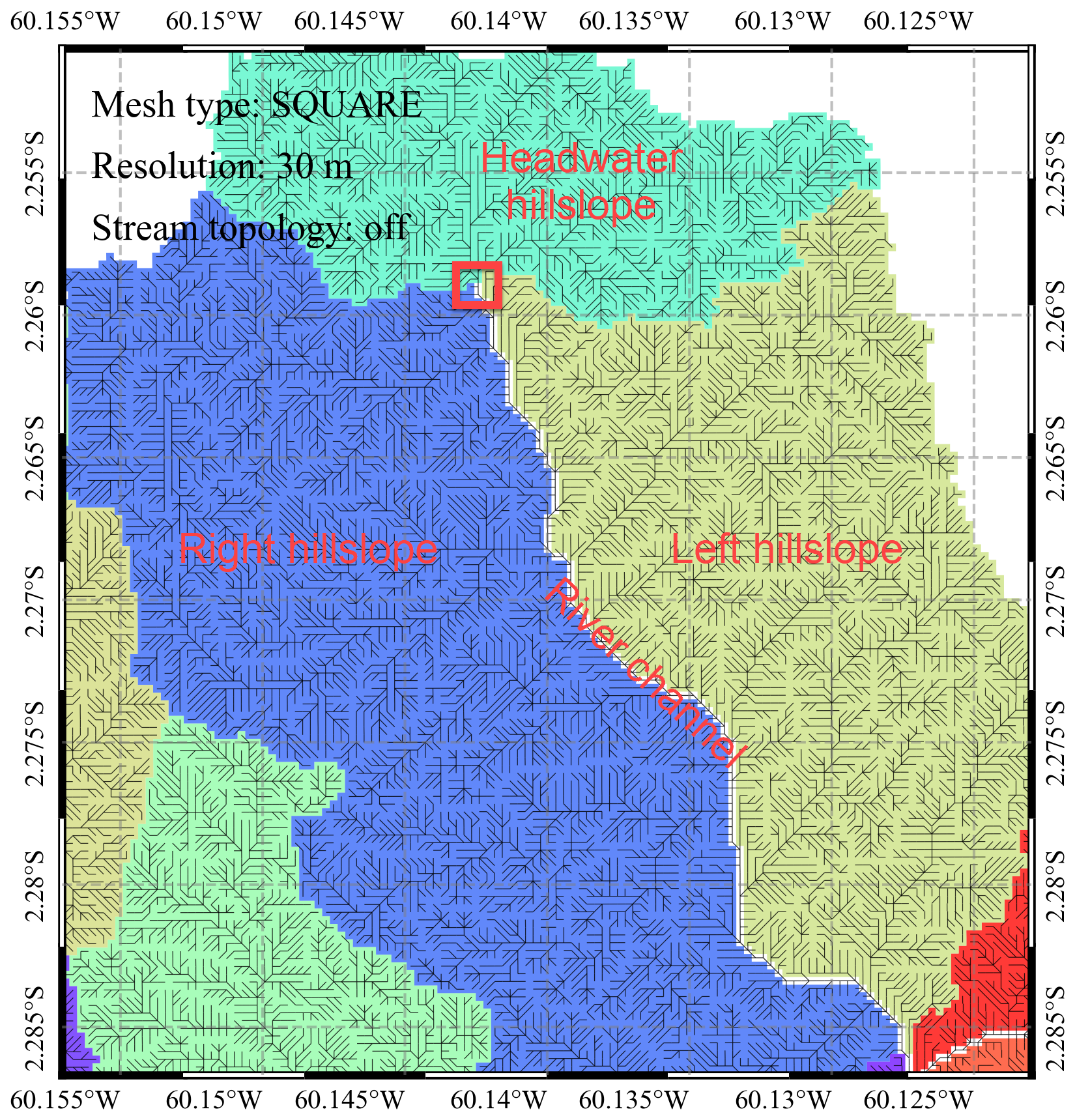
Figure 2 Illustration of the hillslope definition. The colored polygon features are the delineated hillslopes. The white-colored polyline segment in the middle is a delineated river channel by HexWatershed. The black lines from cell to cell are the flow direction field. The river channel is linked to three hillslopes. All the cells entering from the left/right side (upstream facing downstream) of the river channel are grouped as left/right hillslopes. All the cells entering the river channel through the first river channel cell (highlighted in red rectangle) are grouped as the headwater hillslope. The results are produced using the HexWatershed model with 30 m DEM. Map visualization is supported by the PyEarth Python package (Elson et al., 2023; Liao, 2022b).

In the first step, i.e., watershed delineation, a flow accumulation or drainage area threshold is required, and this threshold will affect the total number of stream segments and, thus, the total number of hillslopes. Therefore, we ran this step with different thresholds to evaluate the sensitivity of the hillslope definition to this threshold. Hereafter, this threshold is also referred to as P_drai. Although this approach produces a network of hillslopes, they cannot be represented individually; instead, an averaged “representative” hillslope is used. Details of this approach are provided in the Supplement.

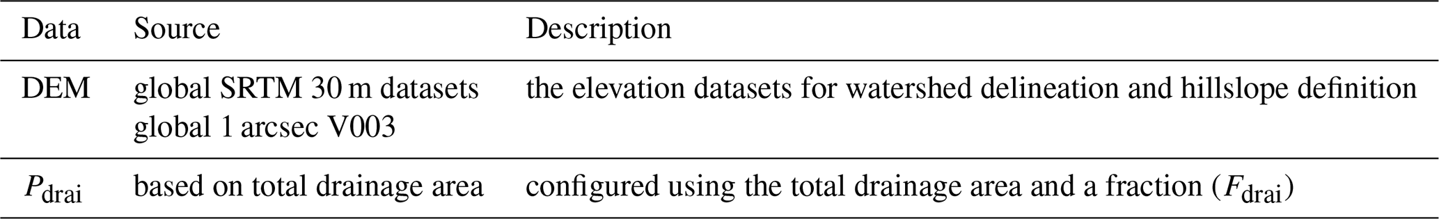
In the second approach, we define the hillslope based on the elevation information from MOSART (Luo et al., 2017, Table 1). Specifically, we use the MOSART elevation profile generated from high-resolution DEM datasets to define the hillslopes and their geometric characteristics. In this approach, we assume there are two facing hillslopes connecting to the main channel, and their attributes are defined using the grid cell dimensions.

Table 1 Definition of hillslope characteristics based on MOSART elevation profile (Luo et al., 2017). Area_g and Length_cell are the area and length of an ELM grid cell; Elev_max and Elev_min are the maximal and minimal elevation from the MOSART elevation profile (Li et al., 2013).

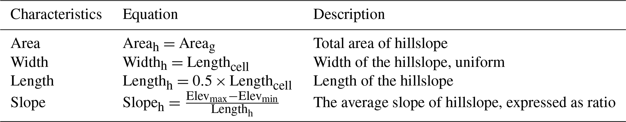
Because neither approach specifies the vertical depth of hillslopes, we define the vertical profile based on the vertical discretization of the ELM soil component (Oleson et al., 2013).

2.2.2 Lateral groundwater flow model

Our numerical model simulates the one-way lateral flow flux from the hillslopes to their connected river channels. In a normal scenario, when the shallow groundwater table along the hillslope is below the land surface, the subsurface lateral groundwater flows through the “downslope end” into the river channel, as illustrated by Fig. 3.

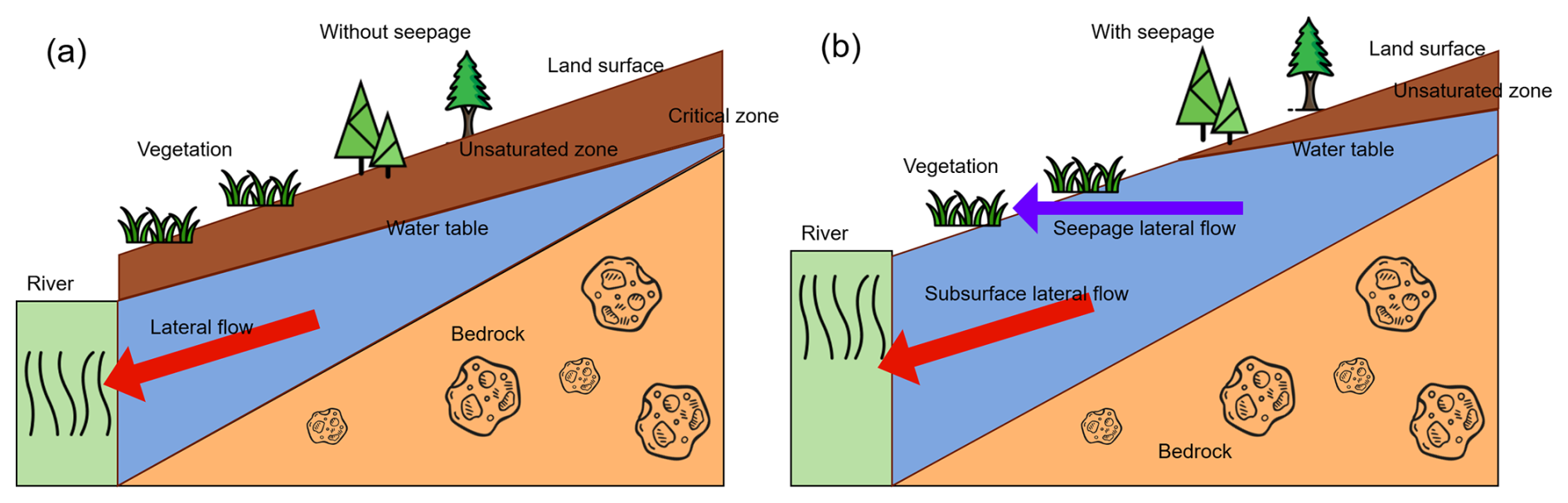
Figure 3 Illustration of the water table and lateral flow along the hillslope (a) without and (b) with a seepage face. When the water table along the hillslope is below the land surface, subsurface lateral groundwater flows through the downslope interface with the river channel. When a portion of the water table is above the foothill of the hillslope, the lateral flow includes both subsurface flow through the downslope interface and seepage flow through the seepage face. Elevation and distance are not drawn to scale.

Below, we first introduce several basic assumptions. Then, we provide more model details.

1. We assume that the hydraulic gradient along a conceptual hillslope equals the water table gradient and is constrained by the time-invariant surface slope and bedrock slope.

2. We assume that surface and bedrock slopes along the hillslope are linear. Besides, because the water table generally follows the surface topography, its gradient is also assumed to be linear and can be expressed as the water table slope.

3. We assume that the critical zone thickness, the distance between the land surface and bedrock, is generally more prominent at lower elevations. As a result, the bedrock slope is slightly larger than the surface slope. A variable-thickness critical zone configuration may further improve the bedrock slope representation.

4. We assume the water table in unconfined aquifers always stays at or above the bedrock. Although the water table generally follows the topography, its slope cannot be larger than the surface slope. This is consistent with other studies (Maquin et al., 2017) and our in situ well measurements.

5. Because surface slope, bedrock slope, and water table slope are all linear, we assume that the change in water table and its slope can be defined using three “shape” parameters (λ₀, λ₁, and λ₂). The first shape parameter λ₀ (Eq. A1) defines the water table slope when the lower end of the water table meets the lower end of the hillslope, which is the transitional scenario between with and without a seepage (Brown line in Fig. A3). The second λ₁ (Eq. A7) and third λ₂ (Eq. A16) shape parameters each describe the nonlinear change in the water table slope based on the transition slope and surface or bedrock slope (green and blue lines in Fig. A3). More details of this design are illustrated in the Supplement (Sect. A1).

The subsurface LGF flux can be calculated by (Maquin et al., 2017)

$$\begin{array}{}\text{(5)}& Q_{\mathrm{lateral}}=Q_{\mathrm{downslope}}={\displaystyle \frac{K_{\mathrm{h},\mathrm{sat}}\times H_{\mathrm{r}}\times \tan \left(S_{\mathrm{wt}}\right)}{L_{\mathrm{hillslope}}}},\end{array}$$

where Q_downslope is the water flow from the downslope end (mm s⁻¹) normalized to the grid area, K_h,sat is the horizontal saturated hydraulic conductivity (mm s⁻¹), and H_r is the groundwater aquifer thickness at the downslope end (mm). H_r is calculated from soil thickness, river channel geometry, and river gage height, and the latter is produced by the MOSART. S_wt is the slope of the water table along the hillslope, and L_slope is the horizontal length of the hillslope (mm). Because ELM uses a multiple-soil-layer scheme, the horizontal saturated hydraulic conductivity can be calculated by a thickness-weighted harmonic mean:

$$\begin{array}{}\text{(6)}& {\displaystyle }& {\displaystyle }{K}_{\mathrm{h},\mathrm{sat}}=\sum _{i=j}^n{\displaystyle \frac{K_{\mathrm{h},\mathrm{sat},i}\times h_i}{\sum _{i=j}^n{h}_i}},\text{(7)}& {\displaystyle }& {\displaystyle }{K}_{\mathrm{anis},i}={\displaystyle \frac{K_{\mathrm{v},\mathrm{sat},i}}{K_{\mathrm{h},\mathrm{sat},i}}},\end{array}$$

where h_i is the thickness of the ith soil layer; $K_{\mathrm{v},\mathrm{sat},i}$ and $K_{\mathrm{h},\mathrm{sat},i}$ are the ith soil layer vertical and horizontal saturated hydraulic conductivity, respectively (mm s⁻¹); K_anis,i is the ith soil layer vertical-to-horizontal anisotropy ratio of saturated hydraulic conductivity; j is the index of where the water table is located; n is the bottom soil layer index. Once the subsurface LGF is calculated, the ELM soil hydrologic status, including the water table, is updated.

In other scenarios, a portion of the water table is at the land surface. A seepage face will emerge, and the LGF is the sum of water flow from the downslope end and the seepage face and can be calculated by the following (Maquin et al., 2017) (Fig. 3).

$$\begin{array}{}\text{(8)}& {\displaystyle }& {\displaystyle }{Q}_{\mathrm{downslope}}={\displaystyle \frac{K_{\mathrm{h},\mathrm{sat}}\times H_{\mathrm{r}}\times \tan \left(S_{\mathrm{surface}}\right)}{L_{\mathrm{hillslope}}}}\text{(9)}& {\displaystyle }& {\displaystyle }{Q}_{\mathrm{seepage}}={\displaystyle \frac{K_{\mathrm{h},\mathrm{sat}}\times L_{\mathrm{seepage}}\times \tan \left(S_{\mathrm{surface}}\right)}{L_{\mathrm{hillslope}}}}\text{(10)}& {\displaystyle }& {\displaystyle }{Q}_{\mathrm{lateral}}=Q_{\mathrm{downslope}}+Q_{\mathrm{seepage}}\end{array}$$

Here S_surface is the surface slope, and L_seepage is the horizontal length of the seepage face (mm).

In rare scenarios, the water table can be higher than the highest elevation of the hillslope, and the entire grid cell is flooded (Fig. A1). In this scenario, an advanced approach is needed to model the interactions between the river and its floodplain.

To model the water table slope, HLGF considers several factors based on several existing studies (Maquin et al., 2017). First, the transition between different water table scenarios must be continuous and not intersect (Fig. A2). Second, when there is no seepage face, the increase or decrease in the water table is slower at lower elevations. Third, when there is a seepage face, the increase or decrease in the water table is slower at high elevations. Lastly, the water table may intersect with bedrock at higher elevations. To summarize, the water table dynamics are illustrated in Fig. A3.

HLGF considers the impact of river gage height on the water table slope. Specifically, it uses time-variant river gage height to calculate the gradient of the water table and aquifer thickness (Fig. 3). The model requires that river water surface and the groundwater water table are the same at the hillslope–river interface. As a result, the aquifer thickness is always less than the thickness of the critical zone and fluctuates with the river gage height. However, because the current version of HLGF only supports a single hillslope, the water table slope is always positive, and the river is always a “gaining” stream.

Since the HLGF model only sends one-way lateral flow from ELM to MOSART, MOSART can operate in either active or data mode. Additionally, because the infrastructure to transmit MOSART status, such as river gage height, back to ELM is not yet available in E3SM, a new data type (“rof2lnd”) was introduced to transfer river status through the CIME coupler.

As many studies suggested, preferential flow plays an important role in ecosystems with intense biological activities that allow macropore flow to bypass the soil columns, thus significantly influencing the partition of surface and subsurface runoff (Beven and Germann, 1982; Cheng et al., 2017). To account for this effect, we implemented a simple macropore flow method. This method uses a macropore fraction parameter (F_macro) to bypass a portion of the surface infiltration directly to the river networks.

3 Model application and evaluation

Most parameters within HLGF are obtained or estimated directly from ELM (Eq. 6). The soil anisotropy (K_anis) of hydraulic conductivity is prepared using the soil sand and clay content (Fan and Miguez-Macho, 2011). The three shape parameters (K₀, K₁, and K₂) that are used to estimate the water table slope are set as 0.5, 1.1, and 0.9 using trial and error approach (Sect. A1).

3.1 Model application

3.1.1 Study area

Following the earlier work of Fang et al. (2022), we defined a standard 0.5°×0.5° ELM grid cell enclosing the field measurement site. This site is located at −60.2093 longitude and −2.6091 latitude (Fig. 4). At this location, the surface elevation is approximately 130 m, and the mean annual precipitation is estimated to be 2252 mm yr⁻¹ (https://ameriflux.lbl.gov/sites/siteinfo/BR-Ma2, last access: 6 November 2023) (Negron-Juarez et al., 2011; Li et al., 2023). Near this site, in situ groundwater well measurements along a hillslope transect and their approximate distances to the nearest river channel are available. We also obtain the DEM dataset from the Shuttle Radar Topography Mission (SRTM) datasets at 30 m (NASA, 2013).

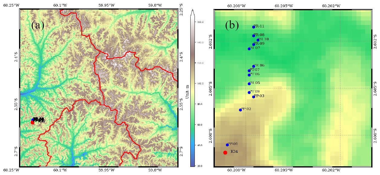
Figure 4 Surface elevation of the study area (unit: m) and locations of in situ measurement sites. Panel (a) is the 30 m resolution surface elevation of the 0.5°×0.5° ELM grid cell. The red lines are watershed boundaries. Panel (b) is a zoomed-in view of the hillslope transect.

3.1.2 Experimental design

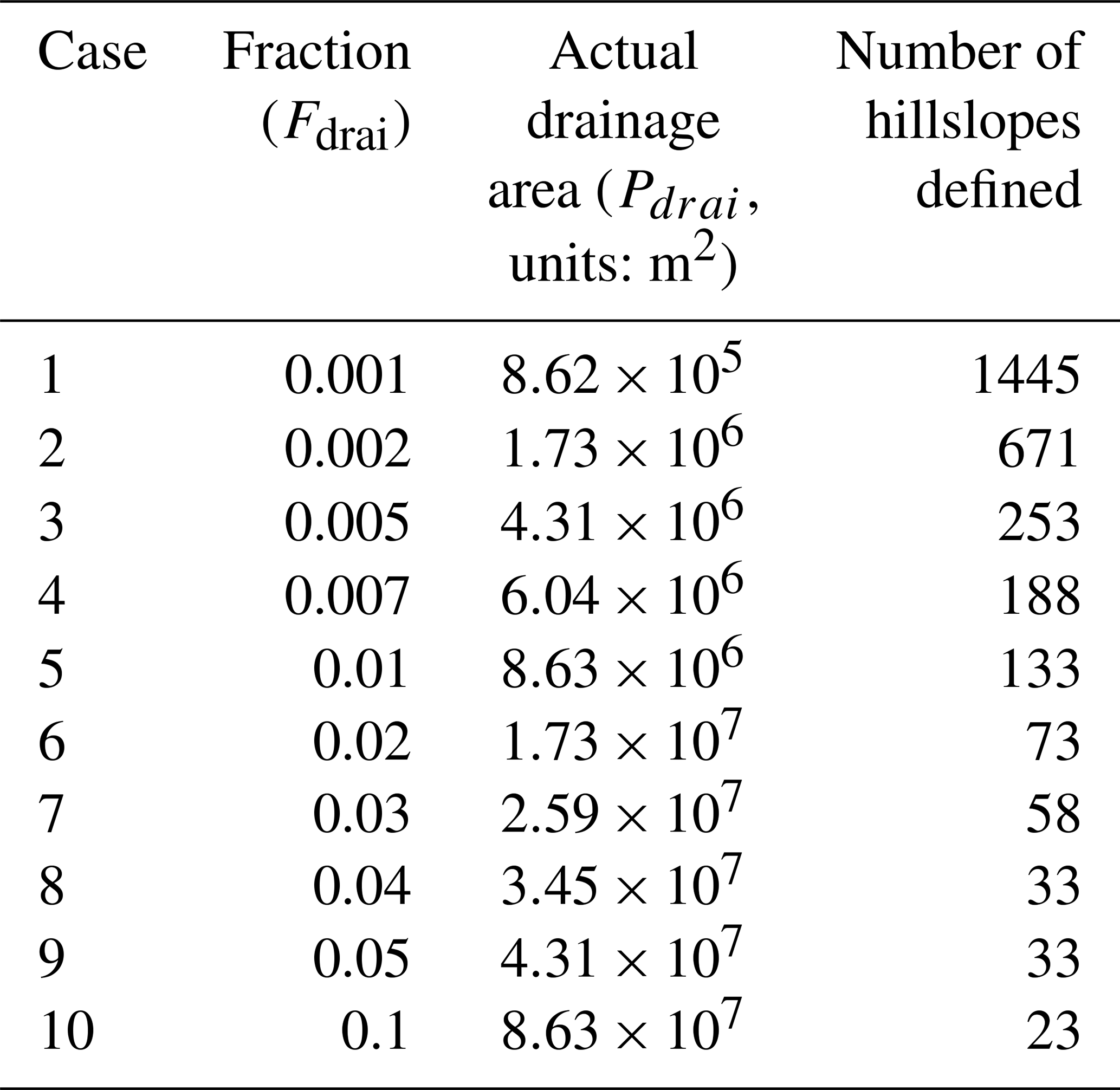
We conducted a range of simulations to investigate the model behaviors using two steps. First, we evaluated the sensitivity of the hillslope definition to the drainage area threshold. Specifically, we ran the HexWatershed model with different drainage area thresholds in the study area and compared the modeled (left, right, and headwater) hillslope geometric characteristics (Table 2). After that, we selected the drainage area threshold resulting in a river network closely resembling the HydroSHEDS river flowline (Lehner and Grill, 2013) as the baseline (Case 3 in Table 2) to set up the HLGF model simulations.

Table 2 HexWatershed simulation configurations with indices. The actual drainage area is calculated as the product of the maximum and fraction drainage area.

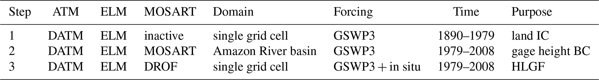
Second, a customized E3SM compset was created for the study area. This customized compset allows the E3SM Atmosphere Model (EAM) and river (MOSART) components to be run in data mode, i.e., DATM and DROF, serving as the upper and lateral boundary conditions (BCs) for the land component ELM. We ran the model simulations using the following steps (Table A1):

1. We ran a 90-year default ELM (ELM+DATM) simulation for the study area to provide a consistent initial condition.

2. We ran another 30-year (1979–2008) default ELM-MOSART (ELM+MOSART+DATM) simulation for the whole Amazon River basin to generate the river gage height BC. The forcing data used to run the ELM and MOSART simulations were obtained from the Global Soil Wetness Project Phase 3 (GSWP3) datasets (Department of Civil and Environmental Engineering, 2006).

3. We ran a 30-year (1979–2008) simulation using our newly developed HLGF model (ELM+DATM+DROF) with different configurations. These configurations include different hillslope definition methods and parameters (Tables 2 and 3).

Table 3 E3SM simulation configurations with case indices.

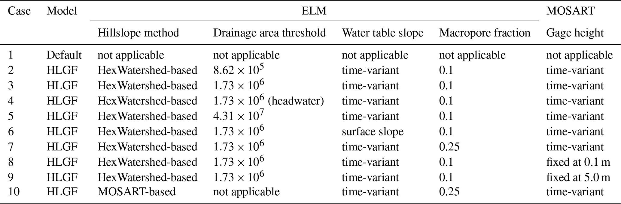
Case 1 is the default ELM simulation. Case 2 is the reference HLGF simulation with the baseline hillslope definition. Cases 3 to 5 investigate the roles of drainage area threshold and, subsequently, surface slope in the HLGF model. Cases 6 to 9 investigate the roles of water table slope (Case 6), preferential flow (Case 7), and river gage height (Cases 8 and 9) in the HLGF model. Case 10 is based on the MOSART hillslope definition. We use observational datasets, i.e., WTD, to evaluate the model performance.

3.2 Model results and analysis

3.2.1 Overview

We first analyze the impact of the drainage area threshold on the hillslope definition, focusing on several geometric characteristics, including hillslope length and slope. Then, we focus on the impacts of surface/water table slopes, river gage height, and preferential flow on the LGF and WTD. Specifically, we compared the differences in LGF and WTD in different model configurations (Table 3). For WTD, we also focused on the differences along the hillslope. For temporal analysis, we focus primarily on the representative months of February and August, corresponding to the wet and dry seasons, respectively.

3.2.2 Hillslope definition

As the drainage area threshold increases, the number of modeled river segments decreases and so does the number of modeled hillslopes (Table 2, Fig. 5). For example, when P_drai is 1.72×10⁶ m² and 8.63×10⁷ m², the model defined 671 and 23 hillslopes, respectively. For comparison, in the MOSART elevation-profile-based method, we can only define 2 hillslopes.

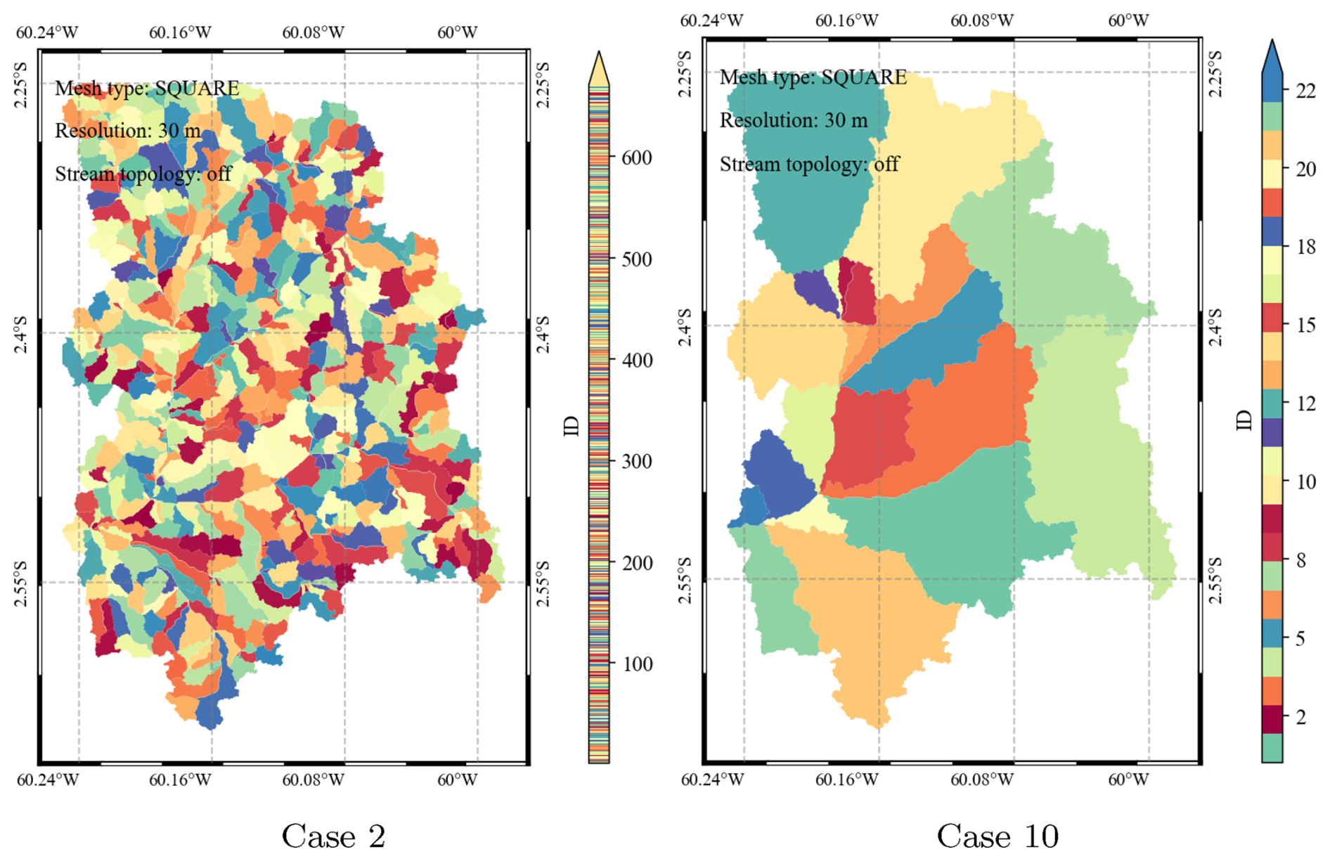
Figure 5 HexWatershed-modeled hillslopes from Cases 2 and 10 (Table 2). The color bar represents the ID of each hillslope. The model defines more hillslopes when the drainage area threshold is smaller.

Besides, the geometric characteristics of modeled hillslopes vary significantly. First, the individual hillslope areas increase by several orders of magnitude, and there are much larger variations when there are fewer hillslopes (Fig. B1). Second, the modeled hillslope length increases as the drainage threshold increases. The average length is around 1 km when P_drai is 1.7×10⁶ m², whereas this is more than 3 km when P_drai is 8.63×10⁷ m² (Fig. 6). Overall, the modeled hillslope lengths are still slightly greater than those reported in earlier studies (Grieve et al., 2016). Third, the modeled hillslope width increases as the drainage threshold increases, except for the headwater hillslopes (convergence at the first cell of the river channel) (Fig. B2).

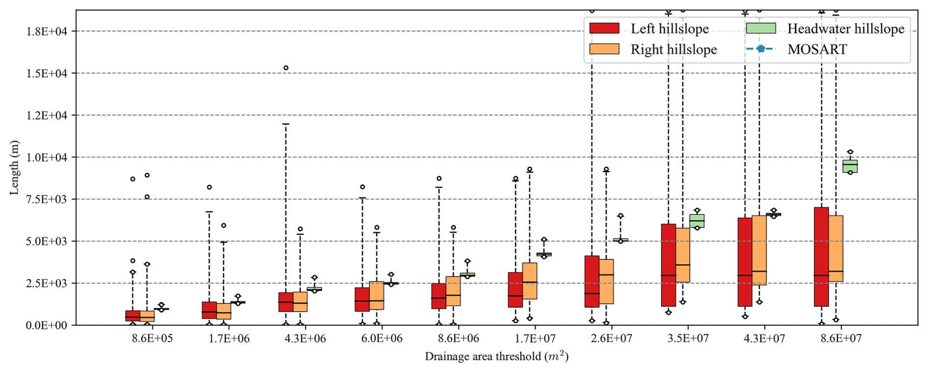
Figure 6 Boxplot comparisons of HexWatershed-modeled hillslope length from Cases 1 to 10 (Table 2). The x axis represents different drainage area thresholds. Each box group includes left, right, and headwater hillslope. The MOSART elevation-profile-based length is out of the range.

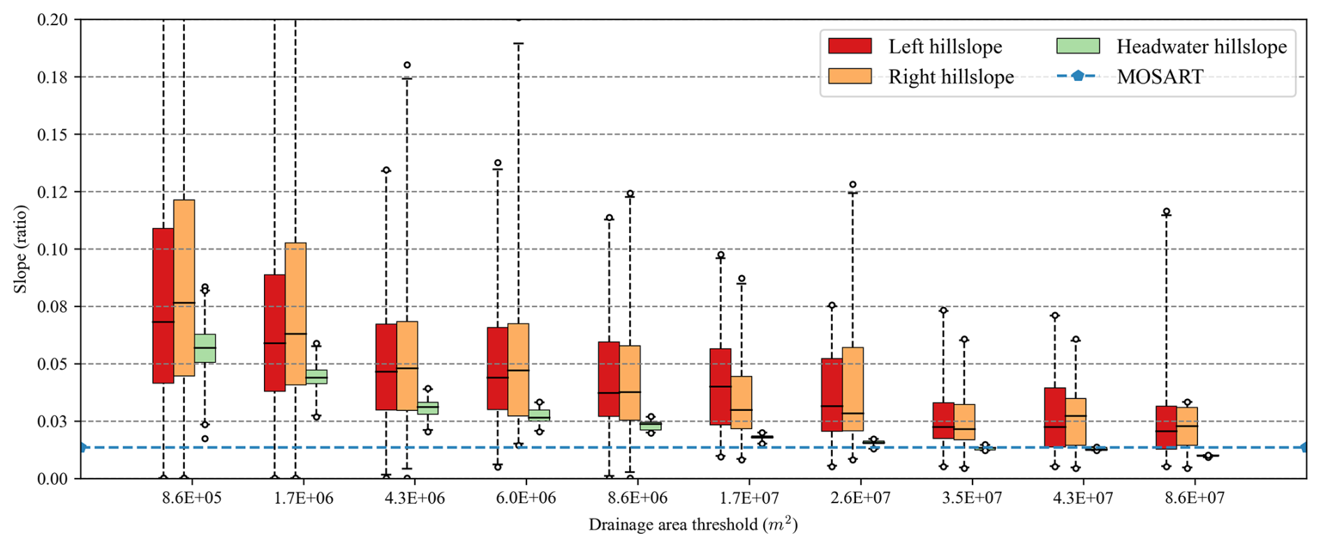
Lastly, the modeled hillslope slope decreases as the drainage threshold increases. When P_drai is small, i.e., at 1.7×10⁶ m², the modeled average slope (∼0.07) is close to the in situ measurement (∼0.047) at a hillslope transect in the study area. In comparison, the modeled hillslope slopes are mostly larger than the MOSART elevation-profile-based slope (∼0.014, dashed blue line in Fig. 7).

Figure 7 Boxplot comparisons of HexWatershed-modeled hillslope slopes from Cases 1 to 10 (Table 2). The x axis represents different drainage area thresholds. Each box group includes left, right, and headwater hillslope. The dashed blue line is the MOSART elevation-profile-based slope.

3.2.3 Lateral groundwater flow

ELM-modeled lateral groundwater flow varies significantly in magnitude and temporal patterns from Cases 1 to 10. First, the default model (Case 1) produced the highest average LGF ($>\mathrm{1.0}\times {\mathrm{10}}^{-\mathrm{4}}$ mm s⁻¹) in February. However, it also produced the lowest average LGF ($<\mathrm{1.0}\times {\mathrm{10}}^{-\mathrm{6}}$ mm s⁻¹) in August (Fig. 8). The pattern is a natural consequence of the power-law behavior within Eq. (1).

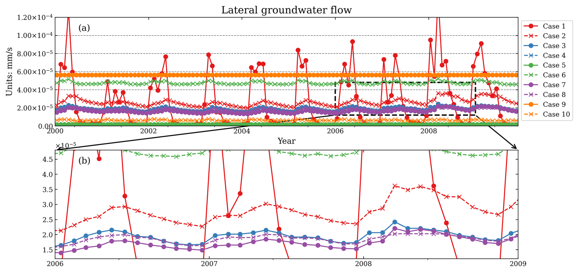
Figure 8 Comparisons of E3SM Land Model (ELM)-simulated monthly lateral groundwater flow from the year 2000 to 2009 from Cases 1 to 10 (Table 3). The x axis is time. The y axis is the lateral groundwater flow (units: mm s⁻¹). Panel (b) is a zoomed-in view of (a) from 2006 to 2009.

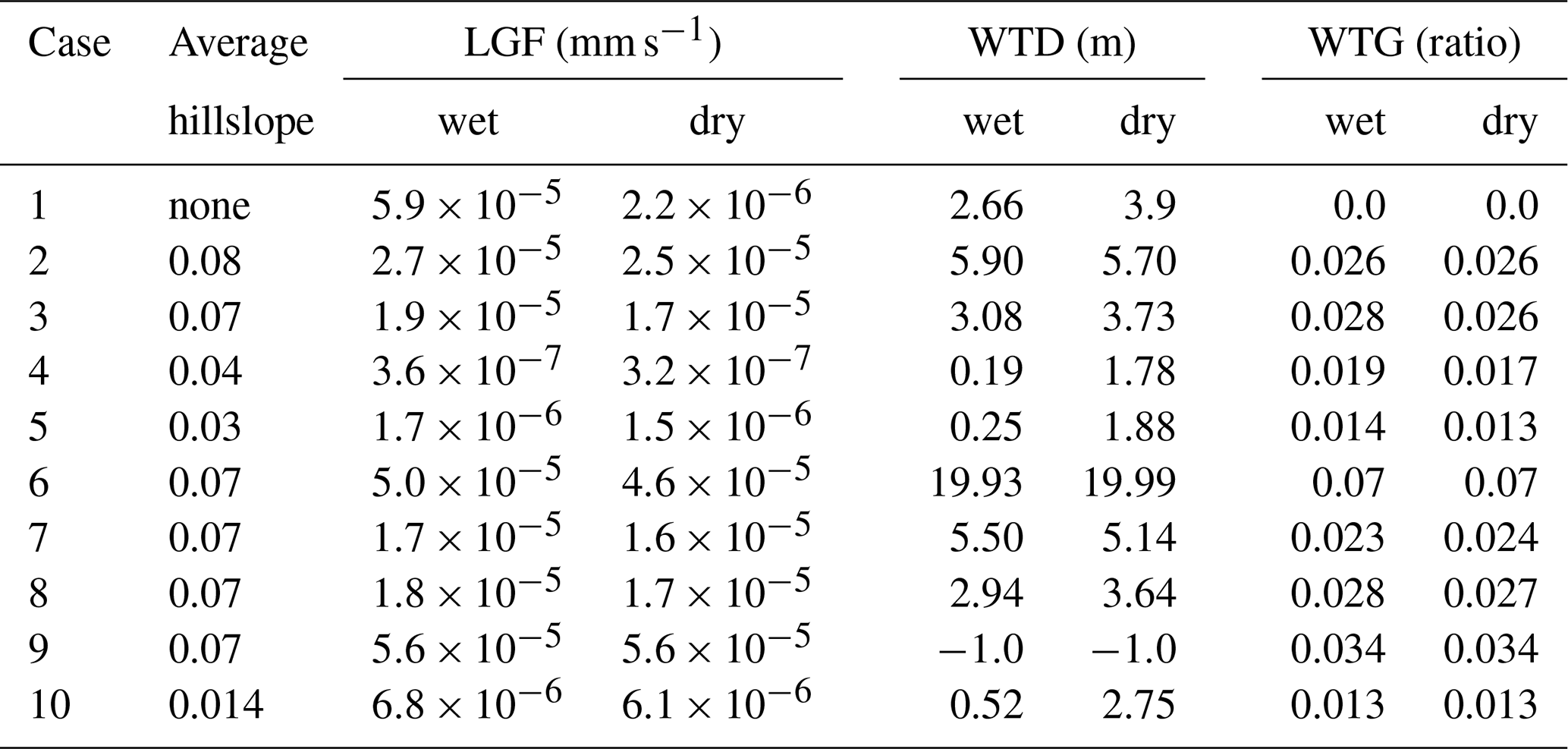
Second, Cases 4, 5, and 10 produced relatively low LGF ($<\mathrm{1.0}\times {\mathrm{10}}^{-\mathrm{5}}$ mm s⁻¹), primarily due to their gentler slopes (0.03 and 0.014) or narrower hillslope widths (30 m) compared to the other cases. Cases 2 to 5 showed that the drainage area threshold can affect the LGF by around 20 % to 40 % (Table 4). Cases 2 and 3 exhibited strong seasonality, and the average LGF is around $\mathrm{2.0}\times {\mathrm{10}}^{-\mathrm{5}}$ mm s⁻¹. In Case 6, the modeled LGF is about twice that of Case 3 when the water table gradient (WTG) matches the slope of the hillslope.

Table 4 E3SM Land Model (ELM)-modeled average lateral groundwater flow (LGF), water table depth (WTD), and water table gradient (WTG) in February (wet) and August (dry) from Cases 1 to 10. The WTG is the gradient of the water table along the hillslope.

Third, Case 7 showed a slight decrease in LGF compared with Case 3, with increased preferential flow. This occurred because higher preferential flow reduced water infiltration into the soil and groundwater systems, thereby limiting the groundwater available for lateral groundwater flow. Lastly, Cases 8 and 9 indicated that river gage height significantly affects LGF. When the interface between the land and river surface water rises, LGF increases 3 times despite slightly increasing the water table gradient. Case 10 has a relatively gentle slope with increased preferential flow. Therefore, its LGF is even smaller than Case 7 (Table 4).

Compared to the default model Case 1, the hillslope-based cases yielded higher LGF in the dry season. For example, the average LGF in Case 3 is $\mathrm{1.7}\times {\mathrm{10}}^{-\mathrm{5}}$ mm s⁻¹, which is more than 5 times that of Case 1 in August. Consequently, the ratio of LGF between the wet and dry seasons in the hillslope-based cases was close to 1.5, indicating relatively consistent LGF across seasons. In contrast, the default Case 1 exhibited a much larger variation (ratio up to 20.0) in LGF between the wet and dry seasons.

3.2.4 Water table depth

ELM simulations revealed significant variations in WTD along the hillslope across Cases 1 to 10. This disparity stems from the inclusion of the hillslope concept in Cases 2–10, while Case 1 (solid red line in Fig. 9) lacks this functionality.

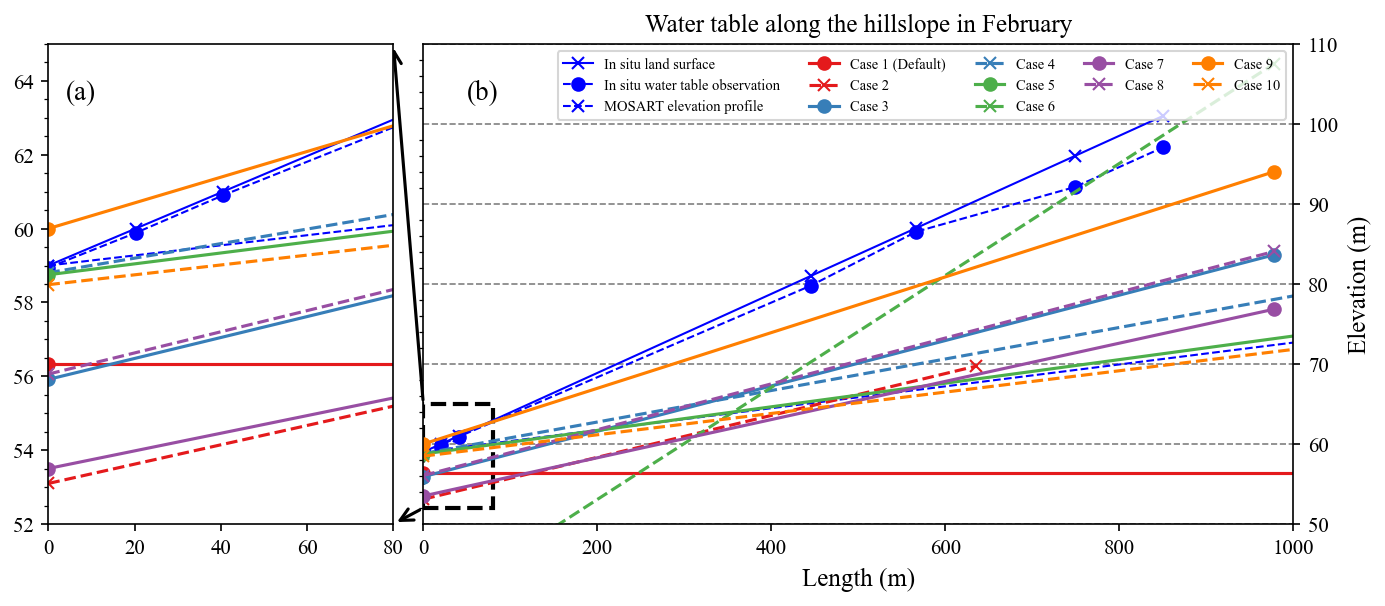
Figure 9 Comparisons of ELM-modeled average water table elevation (surface elevation – water table depth) along the hillslope in February from Cases 1 to 10 (Table 3). The blue lines are in situ observational data and the MOSART elevation profile. The x axis is the distance from the hillslope–river interface (unit: m). The y axis is the elevation (unit: m). The x axis is cut off from the actual hillslope distance to 1000 m for better visualization. Panel (a) is a zoomed-in view near the hillslope–river interface of (b).

In February, the default Case 1 produced a single WTD (∼2.66 m). Case 6 produced the largest average WTD (∼19.9 m) due to the simulated large LGFs ($\sim \mathrm{5.0}\times {\mathrm{10}}^{-\mathrm{5}}$ mm s⁻¹), which itself is caused by high WTG (0.07, equal to surface slope) (Fig. 8 and Table 4). Cases 2 and 7 both produced relatively large average WTDs, approximately 5.9 and 5.5 m, respectively. However, the underlying mechanisms differ. In Case 2, the large average WTD is attributed to a high average WTG (0.026) induced by the hillslope definition (Fig. 7). Conversely, Case 7 exhibited a large average WTD due to reduced infiltration resulting from increased preferential flow bypassing the soil matrix (Table 3).

Cases 3 and 8 behaved similarly for both WTD (∼3.0 m) and WTG (∼0.028). This is because although Case 8 has a constant river gage height, its magnitude (∼0.1 m) is close to the dynamic time series river gage height in Case 3. Case 9 produced the highest average water table (1.0 m above the hillslope–river interface) profile with a seepage face, which was the result of the constant high river gage height (5.0 m). Cases 4, 5, and 10 produced similar average WTDs (<1.0 m) due to their relatively low LGFs (Table 4), which is accompanied by low WTGs (<0.02).

During the dry season, ELM simulations showed a consistent increase in modeled WTDs relative to the wet season (Fig. 10). However, the magnitude of these increases varies depending on the specific case. The default Case 1 produced an increase of 1.3 m in WTD (Table 4). Cases 3 and 8 exhibited a moderate increase of approximately 0.7 m. Cases 4, 5, and 10 displayed a more substantial increase, averaging around 2.0 m. The simulations also showed that the increases in WTD are often accompanied by decreases in WTG. It is important to note that Cases 2 and 7 slightly deviate from this general trend as their WTDs decrease by around 0.2 m compared with the wet season.

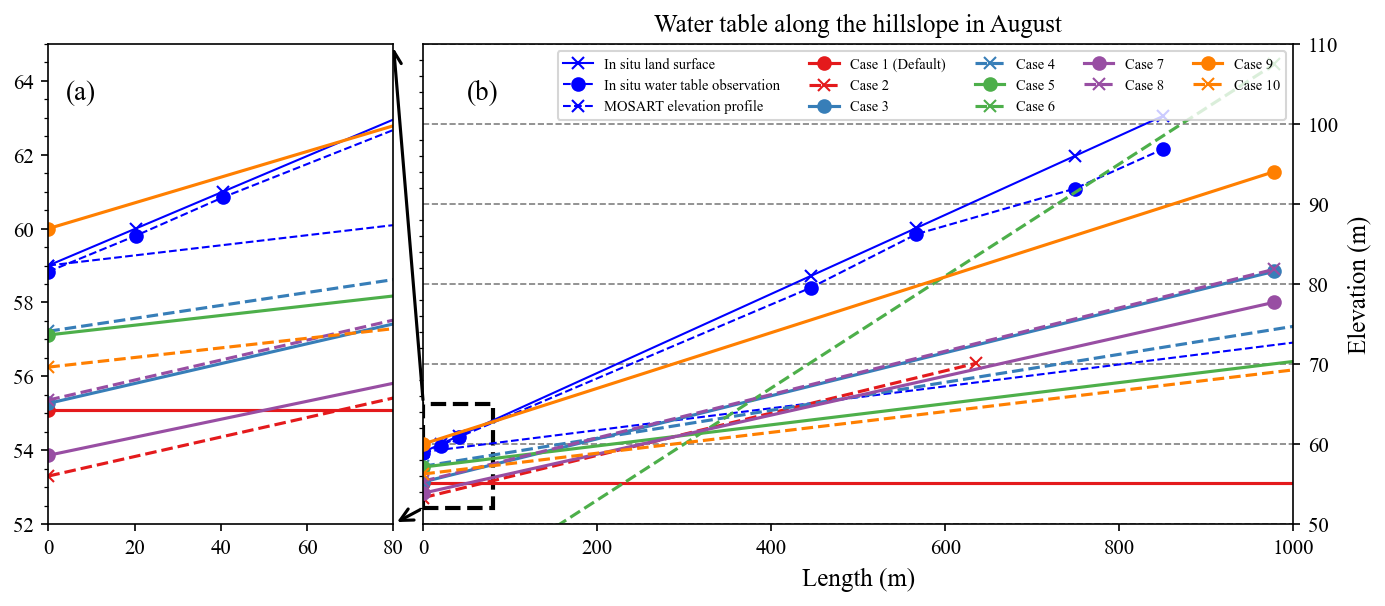
Figure 10 Comparisons of E3SM Land Model (ELM)-simulated average water table elevation along the hillslope in August from Cases 1 to 10 (Table 3). The blue lines are in situ observational data and the MOSART elevation profile. The x axis is the distance from the hillslope–river interface (unit: m). The y axis is the elevation (unit: m). The x axis is cut off from the actual hillslope distance to 1000 m for better visualization. Panel (a) is a zoomed-in view near the hillslope–river interface of (b).

The hillslope-based cases simulated the seasonal fluctuations in WTD and WTG along the hillslope. For example, Case 3 captured the rise and fall of the water table along the hillslope from January to December. The water table profile reaches its highest and lowest points around May and December, the end of the wet and dry seasons, respectively (Fig. 11). The relative relationships of WTD and WTG are also consistent with earlier studies and our model assumptions. Results from other cases are provided in the Supplement (Fig. A4).

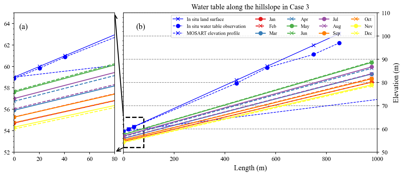
Figure 11 E3SM Land Model (ELM)-simulated average water table depth (WTD) for each month along the hillslope from Case 3 (Table 3). The blue lines are in situ observational data and the MOSART elevation profile. The x axis is the distance from the hillslope–river interface (unit: m). The y axis is the elevation (unit: m). The x axis is cut off from the actual hillslope distance to 1000 m for better visualization. Panel (a) is a zoomed-in view near the hillslope–river interface of (b).

3.2.5 Runoff partition

The simulation results demonstrated that the hillslope model has a significant impact on runoff partitioning. In the default model (Case 1), overland and subsurface runoff account for approximately 34 % and 66 % of the annual total runoff, respectively. Although subsurface runoff contributes nearly twice as much as overland runoff, its contribution varies considerably across seasons. For instance, subsurface runoff can account for up to 72 % in the wet season but drops to just 27 % during the dry season. (Fig. 12).

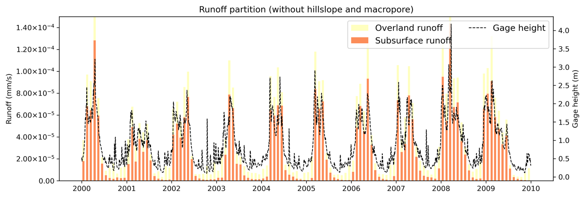
Figure 12 Time series of runoff partition (overland and subsurface runoffs) from the default model Case 1 (Table 3). The x axis is the time. The left y axis is the runoff fluxes (units: mm s⁻¹). The right y axis is the gage height (unit: m).

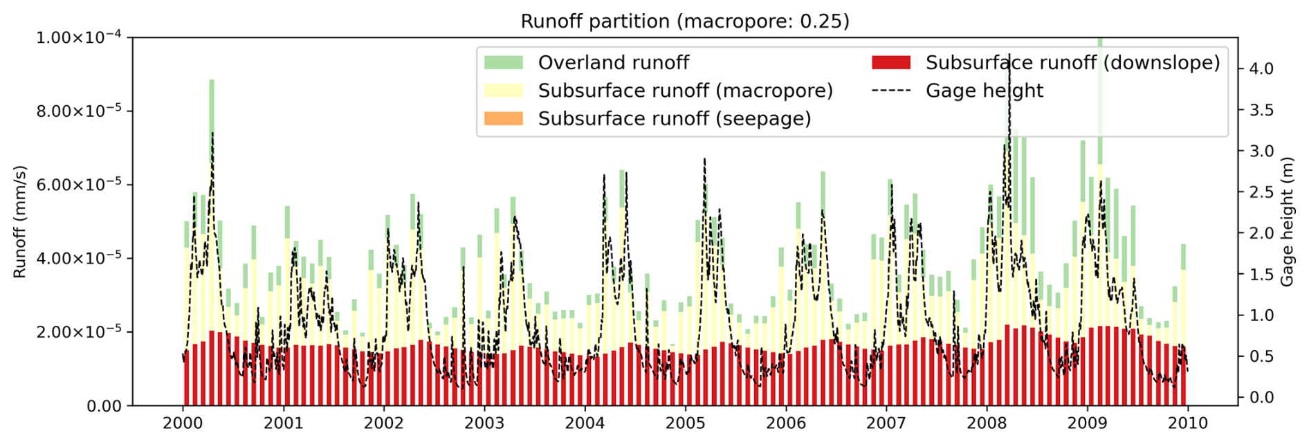
In contrast, in the hillslope-based cases, while the overall contributions from surface and subsurface runoff are similar to those in Case 1, their temporal patterns differ. For instance, in Case 3, subsurface runoff contributes 58 % during the wet season and 80 % in the dry season (Fig. 13). As a result, subsurface runoff becomes the dominant component of total runoff during the dry season.

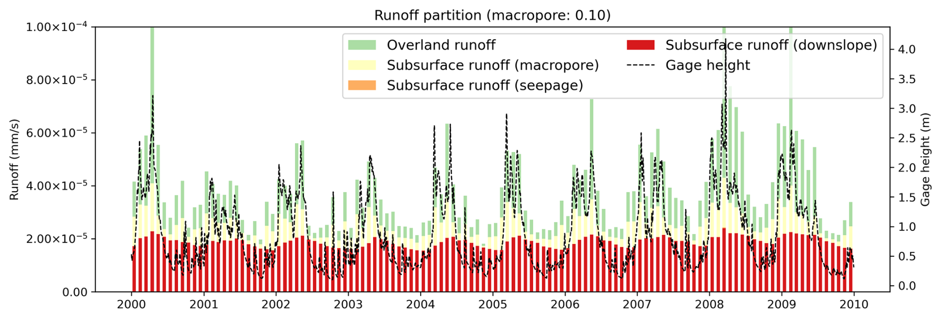
Figure 13 Time series of runoff partition (overland runoff, subsurface runoff from macropore, seepage, and downslope) from the hillslope-based Case 3 (Table 3). The x axis is the time. The left y axis is the runoff fluxes (units: mm s⁻¹). The right y axis is the gage height (unit: m).

Additionally, preferential flow further alters the runoff partition. As the macropore fraction parameter increases, the preferential flow increases and the overland runoff decreases. For example, when the macropore parameter increases from 0.1 to 0.25, its contribution to the total runoff increases from 17 % to 43 %. Meanwhile, the contribution from overland runoff decreases from 34 % to 16 % (Fig. A5). However, the impacts of preferential flow on subsurface runoff from downslope and seepage are not significant.

4 Discussion

4.1 Hillslope characteristics

Our analysis suggests that the definition of hillslopes is a key factor when modeling the lateral groundwater flow at the hillslopes scale. However, accurately defining hillslopes in large-scale hydrologic and Earth system models remains challenging, primarily due to the fractal nature of landscapes, including river networks and hillslopes.

Although land surface modeling has been conducted at spatial resolutions ranging from hundreds of kilometers to meters, there is no consensus on the optimal resolution to capture all key hydrologic processes. Consequently, various simplifications are needed to meet model assumptions. Large-scale hydrologic and Earth system models, with their relatively coarse spatial resolutions, cannot explicitly resolve fine-scale river networks and associated hillslope structures. As a result, these models struggle to accurately represent the geometry (e.g., length, width, slope, aspect) and location of individual hillslopes. Additionally, current ESMs are not equipped to provide spatially explicit vegetation, soil, and climate data at the hillslope scale. Furthermore, natural landscape features like hillslopes often do not align with the artificial boundaries of the meshes used in ESMs, particularly at coarse resolutions where a single hillslope may span multiple grid cells.

A promising solution is the use of high-spatial-resolution or unstructured meshes, which can better capture these natural boundaries. However, this approach requires accounting for lateral flow between cells (both surface and subsurface), in addition to in-channel flow, within ESMs. In summary, without explicitly representing individual hillslopes, existing ESMs cannot accurately simulate lateral groundwater flow or other critical hydrologic processes.

Alternatively, the approach presented in our study offers an initial step toward addressing this challenge. First, it identifies and defines individual hillslopes using high-resolution DEM terrain analysis. Then, a conceptual model, the HLGF model, is applied to simulate hydrologic processes, including lateral groundwater flow, for an “averaged” hillslope. Despite its simplification, this method holds significant potential for enhancing the representation of hydrologic processes on the land surface. While the conceptual hillslope is “averaged”, it effectively captures the dominant characteristics of hillslopes within a large ESM grid cell. Furthermore, individual hillslopes could be directly represented without aggregation if current or future land surface and river-routing models adopt a hillslope-based subgrid structure. Second, our method establishes a natural connection between hillslopes and river networks, enabling two-way interactions between the land surface and river systems. This is achieved through the hillslope definition approach based on the HexWatershed model, where each hillslope is linked to a specific river segment. When provided with dynamic river conditions for different segments, our method can explicitly account for varying hillslope–river interactions.

4.2 Runoff partition

Simulation results from Cases 1 and 3 highlight the significant role of the HLGF model in runoff partitioning. While the annual contributions of lateral groundwater flow to total runoff are similar between the existing model and the HLGF model (both around 66 %), their differences become more pronounced during the wet and dry seasons. For instance, the HLGF-simulated LGFs remain relatively stable across seasons and are the dominant contributor during the dry season (Fig. 13).

In addition, simulation results from Cases 3 and 7 demonstrate the significant influence of preferential flow on runoff partitioning. Preferential flow bypasses the infiltration process, leading to a substantial 18 % reduction in surface runoff. This bypass mechanism also limits the availability of water for lateral groundwater flow, resulting in a less pronounced decrease (8 %) in LGF compared to surface runoff (Figs. A5 and C1).

The integration of hillslope-based groundwater flow (HLGF) and preferential flow models into Earth system models has profound implications for regional water cycles, as these processes directly influence water availability. In drought scenarios, for instance, the HLGF model can provide valuable insights into water table conditions along hillslopes, a critical factor for plant hydraulics and potential tree mortality. Moreover, preferential flow can significantly impact the spatial distribution of soil moisture, both vertically and horizontally, further influencing plant hydraulics.

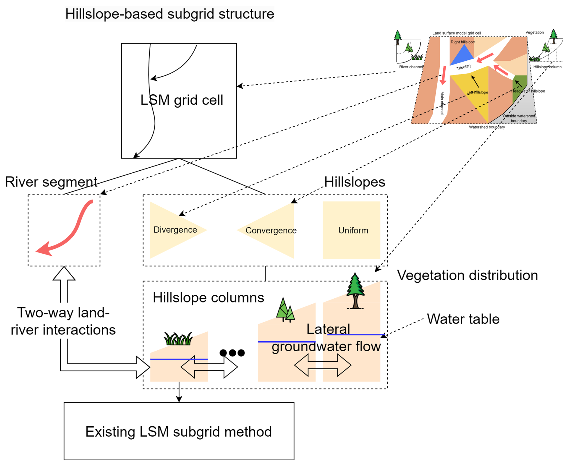
Figure 14 Hillslope-based subgrid structure for land surface models: an LSM grid cell is decomposed into individual river segments and hillslopes. Each hillslope is further subdivided into multiple columns, each representing a distinct vegetation distribution. The interaction between river segments and neighboring hillslopes is facilitated through the lowest-elevation columns. Existing LSM subgrid structures are supported at the column level. The upper-right panel is Fig. 1.

4.3 Groundwater and stream water interactions

The HLGF model provides a physical-based control of lateral groundwater flow, considering land and river water level conditions. This method is robust and can model the seasonal fluctuation in the water table and gradient along the hillslope (Fig. 11). The time series of simulated LGFs from the HLGF model aligns with other studies, reinforcing the notion that subsurface groundwater flow is active throughout the year. This consistency in findings suggests that groundwater may contribute more to river discharge than surface runoff, especially during low-flow seasons.

The HLGF model allows us to explicitly consider groundwater and stream water interactions. However, a challenge remains in representing water table conditions along hillslopes and river channels. First, as a linear feature, the water table along the hillslope varies with location. Therefore, it is advantageous to divide the hillslope into multiple columns so the model can compute the hydraulic head differences between the river and its adjacent land column, i.e., the column with the lowest elevation next to the river channel (Fig. 14). Second, the definition of hillslopes suggests that an average hillslope may not be sufficient to represent the water table conditions in complex landscapes. For example, the main river channel with a low-lying hillslope may be losing water, while a tributary with a steep hillslope may be gaining water (Fig. C1). However, the HLGF model could still be useful if we can represent and model each hillslope separately (Fig. 14). In this scenario, the model can compute the head differences for each hillslope–river pair and the corresponding lateral groundwater flow, which supports both gaining the losing streams simultaneously. Other approaches, such as the Height Above the Nearest Drainage (HAND) model, may also be utilized to link the land surface with the river networks at an even finer scale (Nobre et al., 2011).

5 Limitations

Based on our analysis and discussion, we have identified a few limitations that may be further improved in future studies:

1. While our sensitivity analysis focused on the impact of drainage area on hillslope definition in relation to existing river network datasets, it is essential to acknowledge the presence of both perennial and non-perennial river channels within river systems. Hillslopes can be connected to either type of channel. Therefore, the drainage area threshold, HLGF model, and MOSART model should be equipped to handle non-perennial river channels effectively.

2. The current HLGF model employs a simplified approach that represents hillslopes as a single, linear entity, limiting its ability to capture the intricate topographic heterogeneity often encountered in complex landscapes. Furthermore, the model's inability to simultaneously simulate both gaining and losing streams within a single grid cell restricts its applicability to diverse hydrological scenarios. To overcome these limitations, ESMs should incorporate a hillslope-based subgrid structure within their land and river components. This enhancement would enable the application of the HLGF model to individual hillslopes.

3. Because the HLGF model uses an average hillslope, it cannot accurately describe the divergence or convergence of hillslopes (except the headwater hillslopes), which may introduce large uncertainty in both overland and subsurface flow. To address this, the hillslope-based subgrid structure and an improved divergence or convergence representation method are needed.

4. Our current method only considers all the hillslopes within a single grid cell and ignores the area that is outside of the watershed. Therefore, the lateral groundwater flow may be underestimated when scaling up to the whole grid cell.

5. Given that existing ESMs primarily focus on unconfined aquifers, the HLGF model is currently limited to representing unconfined shallow groundwater systems. To address this constraint and expand the model's applicability, future research should explore and refine the model's structure and functionalities to incorporate confined groundwater systems.

6 Conclusions

We have developed a hillslope-based lateral groundwater flow model, HLGF, to consider the subgrid heterogeneity in topography. This model was implemented in ELM and coupled with MOSART within the E3SM. We applied this model in a 30-year simulation using different configurations to explore how the model responds to various factors such as hillslope definitions and river gage conditions. Our analysis of the results demonstrated that the model is both computationally efficient and effective at simulating water table depth/gradient and runoff partition fluxes along the hillslope. There is still uncertainty due to the differences in scale between hillslopes and the larger-scale ESM grid cells. We believe that this method could be further enhanced by developing a hillslope-based subgrid structure within ESMs to represent fine-scale lateral groundwater flow processes for individual hillslopes.

Appendix A: E3SM and HLGF models

A1 HLGF model algorithms

For a specified hillslope with a slope of S_surface, the model initially calculates the transitional water table slope using the shape parameter λ₀, which ranges from 0 to 1.

$$\begin{array}{}\text{(A1)}& S_{\mathrm{transition}}=S_{\mathrm{surface}}\times {\mathit{\lambda }}_{\mathrm{0}}\end{array}$$

Here S_surface is the surface slope obtained from the hillslope definition (ratio), and S_transition is the transitional water table slope (ratio).

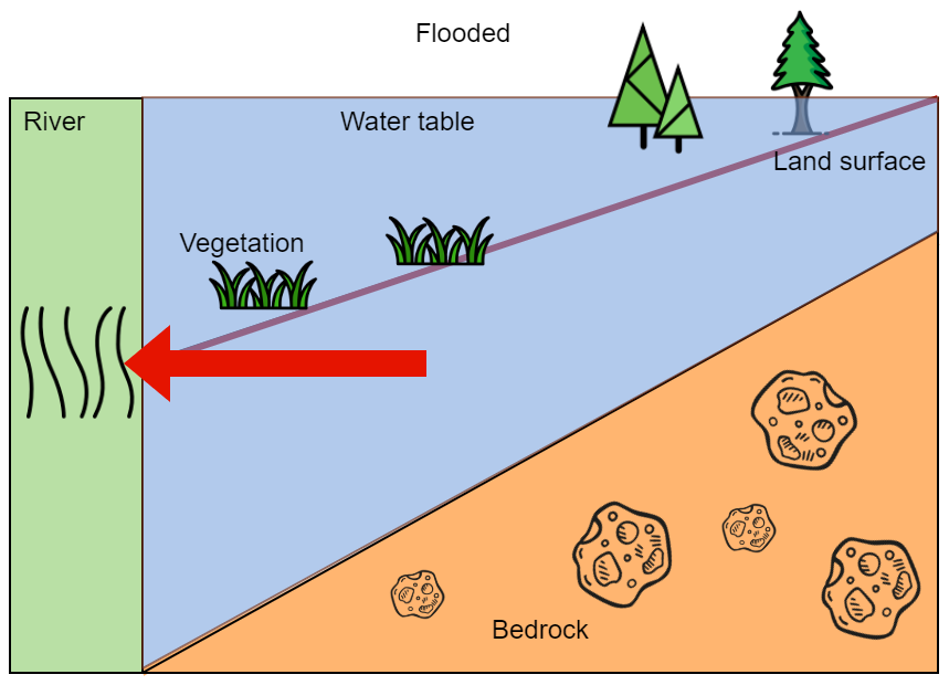
Figure A1 Illustration of water table along the hillslope when the whole grid cell is flooded. Elevation and distance are not drawn to scale.

Following the determination of the transitional water table, the model calculates the water table location under two scenarios. In the first scenario, where the water table is completely below the land surface, the location is determined using three steps.

1. The lower end of the hillslope:

   $$\begin{array}{}\text{(A2)}& {\displaystyle }& {\displaystyle }{\mathrm{Range}}_{\mathrm{low}}={\mathrm{Thickness}}_{\mathrm{low}},\text{(A3)}& {\displaystyle }& {\displaystyle }{\mathrm{Drop}}_{\mathrm{low}}=z_{\mathrm{\nabla }},\end{array}$$
   $$\begin{array}{}\text{(A4)}& {\displaystyle }& {\displaystyle }{\mathrm{Ratio}}_{\mathrm{low}}={\displaystyle \frac{z_{\mathrm{\nabla }}}{{\mathrm{Range}}_{\mathrm{low}}}},\text{(A5)}& {\displaystyle }& {\displaystyle }{\mathrm{Elev}}_{\mathrm{low}}={\mathrm{Elev}}_{\min }-z_{\mathrm{\nabla }},\end{array}$$

   where Range_low is the range of water table change (m), Thickness_low is the (unconfined) aquifer thickness from ELM (m), and Elev_min is the minimal elevation of the hillslope.

2. The higher end of the hillslope:

   $$\begin{array}{}\text{(A6)}& {\displaystyle }& {\displaystyle }{\mathrm{Range}}_{\mathrm{high}}={\mathrm{Thickness}}_{\mathrm{low}}+S_{\mathrm{transition}}\times L_{\mathrm{hillslope}},\text{(A7)}& {\displaystyle }& {\displaystyle }{\mathrm{Ratio}}_{\mathrm{high}}={\mathrm{Ratio}}_{\mathrm{low}}\times {\mathit{\lambda }}_{\mathrm{1}},\text{(A8)}& {\displaystyle }& {\displaystyle }{\mathrm{Drop}}_{\mathrm{high}}={\mathrm{Ratio}}_{\mathrm{high}}\times {\mathrm{Range}}_{\mathrm{high}},\text{(A9)}& {\displaystyle }& {\displaystyle }{\mathrm{Elev}}_{\mathrm{high}}={\mathrm{Elev}}_{\max }-{\mathrm{Drop}}_{\mathrm{high}},\end{array}$$

   where Range_high is the range of water table change (m), L_hillslope is the hillslope length (m), Elev_max is the maximal elevation of the hillslope (m), and λ₂ is the seepage shape parameter.

3. The water table slope:

   $$\begin{array}{}\text{(A10)}& S_{\mathrm{WT}}={\displaystyle \frac{{\mathrm{Elev}}_{\mathrm{high}}-{\mathrm{Elev}}_{\mathrm{low}}}{L_{\mathrm{hillslope}}}}.\end{array}$$

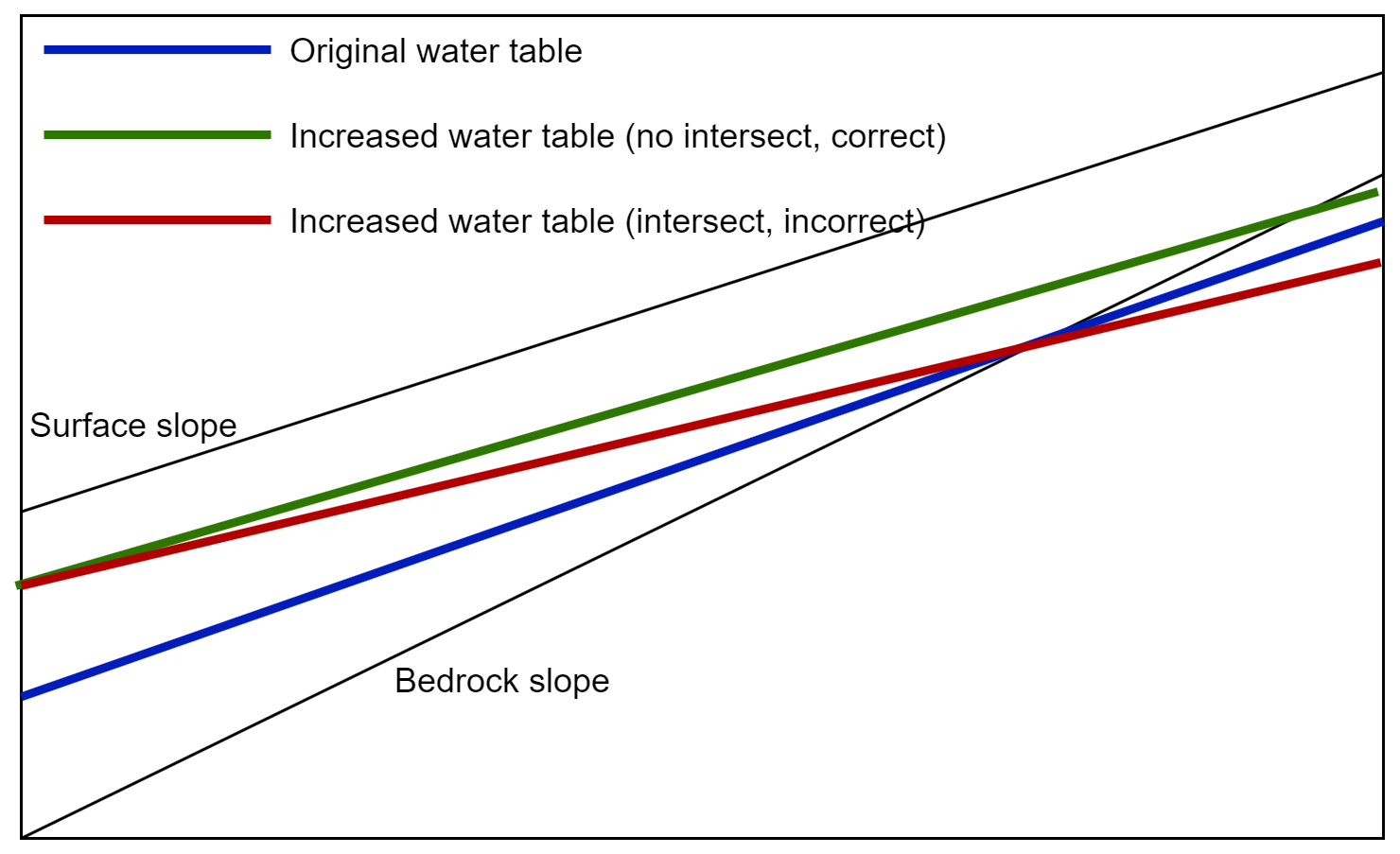
Figure A2 Illustration of water table dynamics along the hillslope without intersect. The blue line represents the initial water table slope. As the water table rises, it should maintain a consistent slope without intersecting previous water table levels, as demonstrated by the green line. The red line, which intersects the blue line, represents an unrealistic representation of water table dynamics.

In the second scenario, where a portion of the water table is above the land surface (indicating seepage), the water table location is calculated using a similar approach.

1. The lower end of the hillslope:

   $$\begin{array}{}\text{(A11)}& {\displaystyle }& {\displaystyle }Rang{e}_{\mathrm{low}}={\mathrm{Elev}}_{\max }-{\mathrm{Elev}}_{\min },\text{(A12)}& {\displaystyle }& {\displaystyle }{\mathrm{Rise}}_{\mathrm{low}}={\mathrm{Elev}}_{\mathrm{wt}}-{\mathrm{Elev}}_{\min },\text{(A13)}& {\displaystyle }& {\displaystyle }{\mathrm{Ratio}}_{\mathrm{low}}={\displaystyle \frac{{\mathrm{Rise}}_{\mathrm{low}}}{{\mathrm{Range}}_{\mathrm{low}}}},\end{array}$$

   where Elev_wt is the water table elevation (m).

2. The higher end of the hillslope:

   $$\begin{array}{}\text{(A14)}& {\displaystyle }& {\displaystyle }{\mathrm{Elev}}_{\mathrm{transition}}=S_{\mathrm{transition}}\times L_{\mathrm{hillslope}}+{\mathrm{Elev}}_{\min },\text{(A15)}& {\displaystyle }& {\displaystyle }{\mathrm{Range}}_{\mathrm{high}}={\mathrm{Elev}}_{\max }-{\mathrm{Elev}}_{\mathrm{transition}},\text{(A16)}& {\displaystyle }& {\displaystyle }{\mathrm{Ratio}}_{\mathrm{high}}={\mathrm{Ratio}}_{\mathrm{low}}\times {\mathit{\lambda }}_{\mathrm{2}},\text{(A17)}& {\displaystyle }& {\displaystyle }{\mathrm{Rise}}_{\mathrm{high}}={\mathrm{Ratio}}_{\mathrm{high}}\times {\mathrm{Range}}_{\mathrm{high}},\text{(A18)}& {\displaystyle }& {\displaystyle }{\mathrm{Elev}}_{\mathrm{high}}={\mathrm{Elev}}_{\mathrm{transition}}+{\mathrm{Rise}}_{\mathrm{high}},\end{array}$$

   where Elev_transition represents the elevation at the top of the transitional water table along the hillslope, and λ₂ is the seepage shape parameter.

3. The water table intersects the land surface at seepage:

   $$\begin{array}{}\text{(A19)}& {\displaystyle }& {\displaystyle }{\mathrm{Elev}}_{\mathrm{intersect}}={\mathrm{Elev}}_{\mathrm{wt}},\text{(A20)}& {\displaystyle }& {\displaystyle }{L}_{\mathrm{intersect}}={\displaystyle \frac{{\mathrm{Elev}}_{\mathrm{wt}}-{\mathrm{Elev}}_{\min }}{S_{\mathrm{surface}}}},\end{array}$$

   where Elev_intersect is the elevation at the top of the seepage (m), and L_intersect is the length of the seepage (m).

4. The water table slope above seepage:

   $$\begin{array}{}\text{(A21)}& S_{\mathrm{WT}}={\displaystyle \frac{{\mathrm{Elev}}_{\mathrm{high}}-{\mathrm{Elev}}_{\mathrm{intersect}}}{L_{\mathrm{hillslope}}-L_{\mathrm{intersect}}}}.\end{array}$$

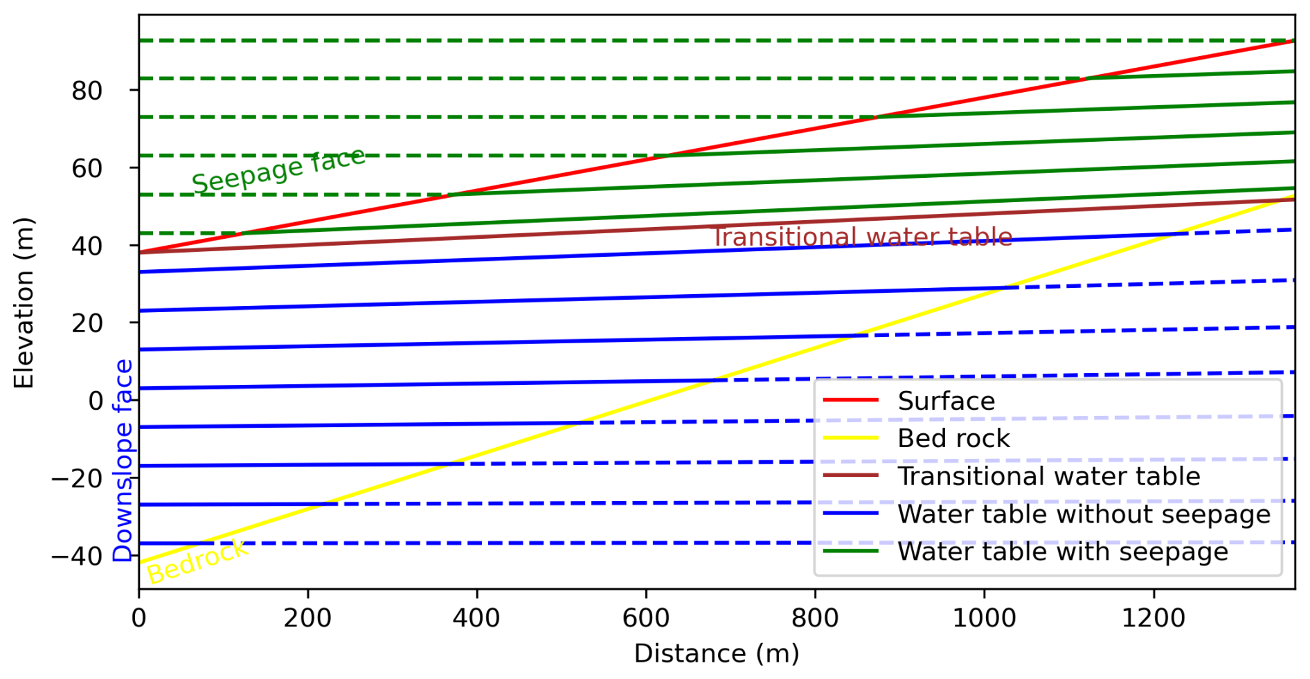
Figure A3 Illustration of water table dynamics along the hillslope. Solid green, brown, and blue lines represent the water table under different scenarios. Dashed lines are used to illustrate the slope and position only. Elevation and distance are not drawn to scale.

A2 E3SM configurations

Table A1 E3SM setups tailored for HLGF model simulations (IC: initial condition; BC: boundary condition).

A3 E3SM results

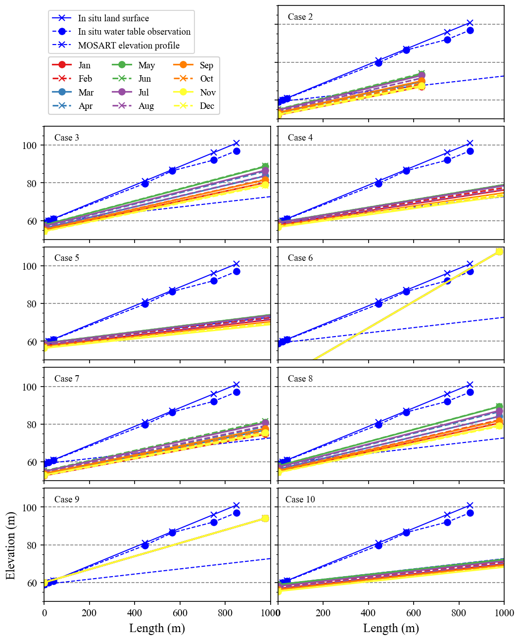
Figure A4 E3SM Land Model (ELM)-simulated average water table depth (WTD) for each month along the hillslope from Cases 2 to 10 (Table 3). The blue lines are in situ observational data and the MOSART elevation profile. The x axis is the distance from the hillslope–river interface (unit: m). The y axis is the elevation (unit: m). The x axis is cut off from the actual hillslope distance to 1000 m for better visualization. Only a few cases (including Case 3) can produce reasonable water table scenarios.

Figure A5 Time series of runoff partition (overland runoff, subsurface runoff from macropore, seepage, and downslope) from the hillslope-based Case 7 (Table 3). The x axis is the time. The left y axis is the runoff fluxes (units: mm s⁻¹). The right y axis is the gage height (unit: m).

Appendix B: Hillslope definition

B1 HexWatershed model algorithms

The HexWatershed model defines the hillslope using the following steps (Steps 1 to 6 are described in Liao et al., 2023):

1. Perform depression removal using the priority-flood algorithm.

2. Determine the dominant flow direction using the steepest slope.

3. Calculate the flow accumulation or upstream drainage area.

4. Define the stream grid using the drainage area threshold.

5. Identify and delineate the stream segments.

6. Establish the boundaries of subbasins and watersheds.

7. To delineate hillslopes, each stream segment is divided into left and right banks. For each mesh cell within a subbasin, its entry point into the stream segment is determined. Mesh cells entering from the left or right riverbank are assigned to the corresponding hillslope, while those entering from the initial stream cell are categorized as part of the headwater hillslope.

B2 HexWatershed model configurations

Table B1 HexWatershed model configurations for hillslope definition.

B3 HexWatershed model results

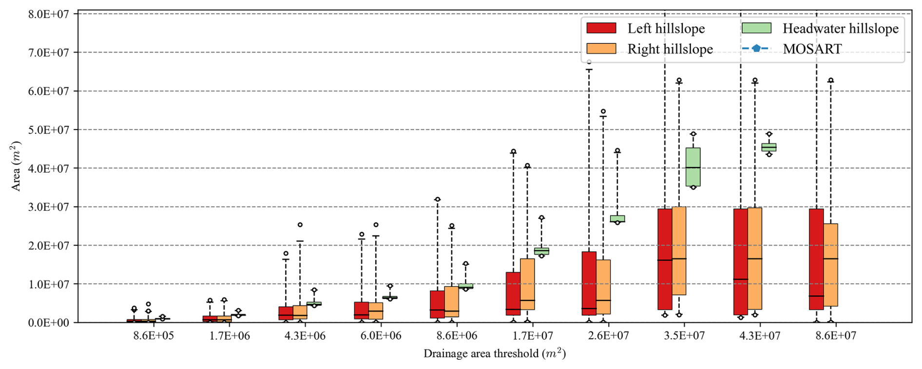
Figure B1 Boxplot comparisons of modeled hillslope area from Cases 1 to 10 (Table 2). The x axis represents different drainage area thresholds. Each box group includes left, right, and headwater hillslope. The MOSART elevation-profile-based area is out of the range.

Figure B2 Boxplot comparisons of HexWatershed-modeled hillslope width from Cases 1 to 10 (Table 2). The x axis represents different drainage area thresholds. Each box group includes left, right, and headwater hillslope. The MOSART elevation-profile-based width is out of the range.

Appendix C: Land–river water cycle interaction

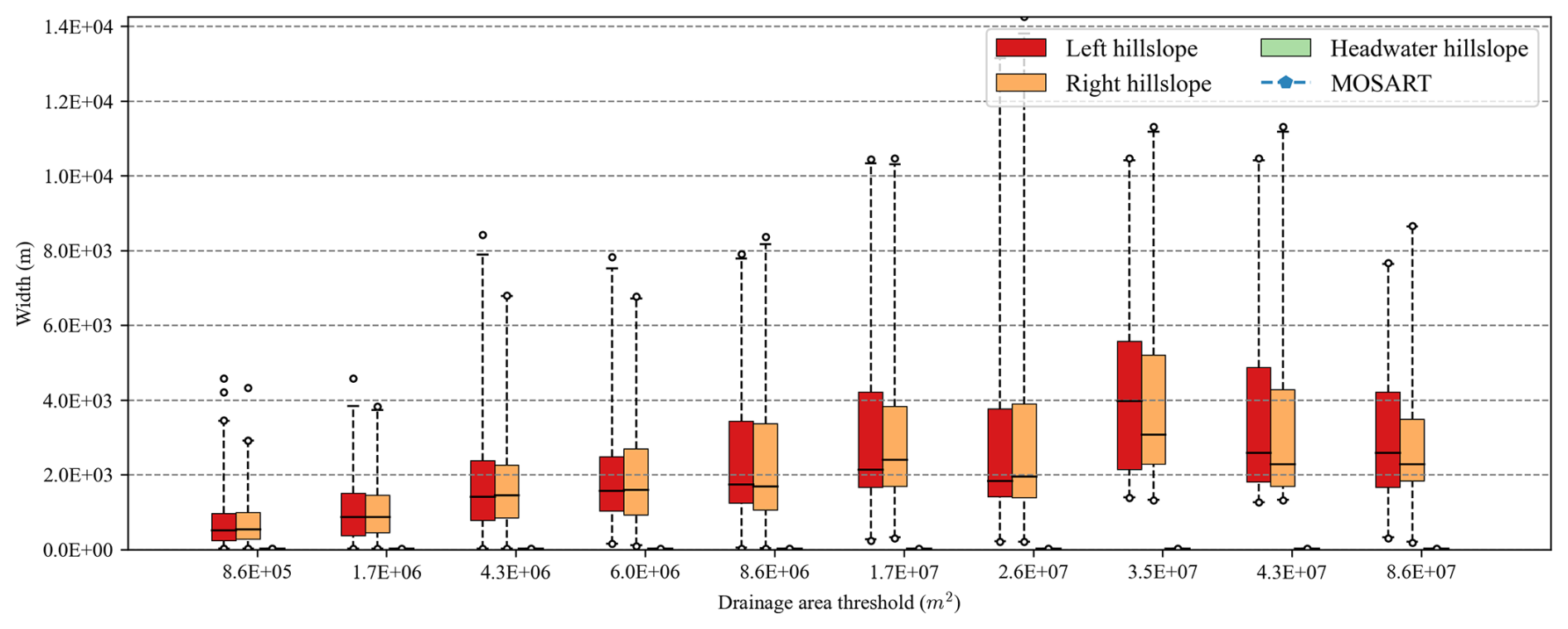
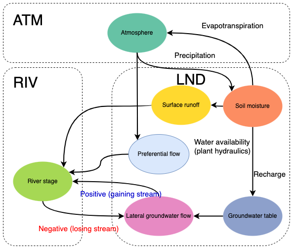
Figure C1 Illustration of land (LND) and river (RIV) surface and groundwater interactions in an Earth system model. The land receives precipitation from the atmosphere (ATM). A portion of the precipitation infiltrates into the soil matrix and recharges the groundwater system. If the soil is saturated on the top layer, excess water forms surface runoff. Another portion of the precipitation bypasses the soil matrix in the form of preferential flow. When there is a hydraulic head difference between LND and RIV, lateral groundwater flow emerges. The direction of lateral groundwater flow depends on the head differences, and the river may gain or lose water.