the Creative Commons Attribution 4.0 License.
the Creative Commons Attribution 4.0 License.
 | 29 Jul 2025
Carbon dioxide plume dispersion simulated at the hectometer scale using DALES: model formulation and observational evaluation
Arseniy Karagodin-Doyennel
Fredrik Jansson
Bart J. H. van Stratum
Hugo Denier van der Gon
Jordi Vilà-Guerau de Arellano
Sander Houweling
Developing effective global strategies for climate mitigation requires an independent assessment of the greenhouse gas emission inventory at the urban scale. In the framework of the Dutch Ruisdael Observatory infrastructure project, we have enhanced the Dutch Atmospheric Large-Eddy-Simulation (DALES) model to simulate carbon dioxide (CO2) plume emission and three-dimensional dispersion within the turbulent boundary layer. The unique ability to explicitly resolve turbulent structures a the hectometer resolution (100 m) makes DALES particularly suitable for detailed realistic simulations of both singular high-emitting point sources and urban emissions, aligning with the goals of Ruisdael Observatory. The model setup involves a high-resolution simulation (100 m × 100 m) covering the main urban area of the Netherlands (51.5–52.5° N, 3.75–6.45° E). The model integrates meteorological forcing from the HARMONIE-AROME weather forecasting model, background CO2 levels from the CAMS reanalysis, and point source emissions and downscaled area emissions derived from the 1 km × 1 km emission inventory from the national registry. The latter are prepared using a sector-specific downscaling workflow, covering major emission categories. Biogenic CO2 exchanges from grasslands and forests are interactively included in the hectometer calculations within the heterogeneous land–surface model of DALES. Our evaluation strategy is twofold, comparing DALES simulations with (i) the state-of-the art LOTOS-EUROS model simulations and (ii) Ruisdael surface observations of the urban background in the Rotterdam area at Westmaas and Slufter and in situ rural Cabauw tower measurements. Our comprehensive statistical analysis confirmed the effectiveness of DALES at modeling the urban-scale CO2 emission distribution and plume dispersion under turbulent conditions but also revealed potential limitations and areas for further improvement. Thus, our new model framework provides valuable insights into the role of anthropogenic and biogenic contributions to local CO2 levels, as well as the transport and dispersion of CO2 emissions. This supports emission uncertainty reduction using atmospheric measurements and contributes to the development of effective regional climate mitigation strategies.
- Article
(11530 KB) - Full-text XML
- BibTeX
- EndNote


Climate change is a critical global environmental problem caused by rising concentrations of carbon dioxide (CO2) and other long-lived greenhouse gases (GHGs) (IPCC, 2021). To address this problem, international agreements like the Paris Agreement aim to mobilize political forces to reduce GHG emissions. Expanding urban areas play a key role, as they account for 60 %–70 % of global CO2 emissions (IPCC, 2023). A recent United Nations Framework Convention on Climate Change (IPCC, 2023) report also highlights the prominent role of urban CO2 emissions in amplifying climate change, underscoring the urgent need to address them in mitigation efforts. However, urban environments pose challenges due to their complex, heterogeneous landscapes; diverse emission sources (e.g., transport, industry, and biosphere interactions); and significant spatiotemporal variability caused by atmospheric turbulence. Tackling these challenges for the quantification of emissions requires high-resolution data to precisely identify emission hotspots, which is crucial for effective monitoring and mitigation.
To address the urgent question of how to reduce emissions most efficiently, many countries have developed national programs for monitoring atmospheric GHG concentrations. Initiatives such as CarboCount-CH (see http://carbocount.wikidot.com/, last access: 27 November 2024) in Switzerland, the GAUGE project in the UK (Palmer et al., 2018), and the European ICOS initiative (see https://www.icos-cp.eu/, last access: 27 November 2024); the North American Carbon Program (see https://www.nacarbon.org/nacp/, last access: 27 November 2024) in the US; and the CONTRAIL project (https://cger.nies.go.jp/contrail/about/index.html, last access: 27 November 2024) in Japan reinforce global efforts to establish transparent and accurate CO2 and CH4 emission tracking.
On the other hand, as cities are major CO2 sources, targeted monitoring is becoming a priority. Due to their complexity and growth, cities require detailed observations and analysis, although monitoring them is particularly challenging (Huo et al., 2022). Programs like ICOS Cities (see https://www.icos-cp.eu/projects/icos-cities, last access: 27 November 2024), Urban-GEMMS (see https://www.arl.noaa.gov/research/atmospheric-transport-and-dispersion/urban-gemms/, last access: 27 November 2024), and the C40 Cities Climate Leadership Group support high-resolution modeling to capture the fine-scale variability in urban emissions. Furthermore, the Megacities Carbon Project (see https://earthobservatory.nasa.gov/images/86970/megacities-carbon-project, last access: 27 November 2024) tracks emissions in global cities, supporting efforts to refine urban GHG inventories and strengthen mitigation policies (Timmermans et al., 2013).
In the Netherlands, there is a similar need. According to the Nationally Determined Contribution climate action plan, the Dutch government aims to reduce CO2 emissions by 55 % by 2030 and achieve climate neutrality by 2050 (UNTC (United Nations Treaty Collection), 2016). Thus, comprehensive studies of urban emission sources and distribution in the environment are essential to meet these ambitious reduction targets. A notable initiative in this regard is that of the Dutch Ruisdael Observatory (see https://ruisdael-observatory.nl/, last access: 27 November 2024). This infrastructure project has been established to improve the accuracy of weather and air quality forecasts in a changing climate and provide society with this high-quality and highly detailed information to address existing climate problems. One of the aims is to model the entire Dutch atmosphere at a 100 m resolution, combining simulations with meteorological and atmospheric composition data.
Despite significant progress in emission modeling at different scales (Sarrat et al., 2007; Meesters et al., 2012; Liu et al., 2017; Super et al., 2017; Brunner et al., 2019; Jähn et al., 2020; Brunner et al., 2023), a critical lack of realistic modeling of urban-scale CO2 emissions still remains. Moreover, capturing sub-kilometer emission plume features, such as dispersion and inherent turbulence effects within the atmospheric boundary layer (ABL), might be important for accurate quantification of emissions. Hence, integrating anthropogenic emission inventories into frameworks like large-eddy-simulation (LES) models (Deardorff, 1972), which explicitly resolve a major part of atmospheric turbulence, addresses this need. Brunner et al. (2023) demonstrated that LES models effectively capture CO2 plume dynamics from coal-fired power plants, highlighting the importance of the model resolution. Thus, despite the computational demands associated with LESs, the development of such a simulation framework has the potential to significantly enhance the ability of models to reproduce the observed CO2 signal in urban areas (Sarrat et al., 2007; Liu et al., 2017; Super et al., 2017; Brunner et al., 2023). Along with that, incorporating a dynamic ecosystem model, which accounts for plant CO2 assimilation and soil respiration, can further enhance urban-scale simulation by means of LESs (Vilà-Guerau de Arellano et al., 2014). Driving the ecosystem model for CO2 fluxes with LESs allows for the resolution of the fine-scale atmospheric processes that influence CO2 exchange with higher accuracy than traditional mesoscale models, which rely on parameterized boundary layer dynamics. LESs can help to resolve the observed rapid meteorological fluctuations in radiation and turbulence (seconds to minutes) that strongly impact fluxes of heat, moisture, and CO2 (see Vilà-Guerau de Arellano et al., 2014). Thus, by explicitly simulating clouds and their effects on diffuse radiation, temperature, and moisture, we can improve the representation of key drivers of photosynthesis and respiration, thereby improving the modeled representation of the biogenic contribution to atmospheric CO2 concentrations.
To achieve high-resolution modeling, detailed emission inventories are essential. Previous studies have provided valuable information on various emission inventories at different scales, from global (Guevara et al., 2019, 2024) to regional (Urraca et al., 2024), and across Europe (Xiao et al., 2021; Kuenen et al., 2022), Asia (Jia et al., 2021), and North America (Brioude et al., 2012), etc. In the Netherlands, for CO2 emissions, the National Institute for Public Health and the Environment (RIVM) provides registered annual individual emission sources from industry, as well as an area emission inventory from various categories mapped to a kilometer-scale grid (https://data.emissieregistratie.nl/, last access: 27 November 2024). However, they are not sufficient for 100 m scale LES models and cannot be employed without proper downscaling. However, this process presents significant challenges due to spatiotemporal uncertainties that emerge when downscaling coarse-resolution data. For point sources, which are supposed to be easier to apply to LESs due to their precise emitting locations, accurate vertical allocation through plume rise is crucial and is not trivial to estimate, although accounting for it is important in simulations (Brunner et al., 2019). Hence, achieving the required level of accuracy in emission modeling involves the complex processes of downscaling in space and time, as well as accurate vertical allocation of emissions.
This need motivates the continued development of related improvements in LES tools and associated national emission inventories. One such model that has been developed for the Netherlands is the Dutch Atmospheric Large-Eddy-Simulation (DALES) model framework (Heus et al., 2010; Ouwersloot et al., 2017). Traditionally, this simulation technique was employed primarily to study atmospheric physics and ABL dynamics (Heus et al., 2010; van Heerwaarden et al., 2017) but not to simulate CO2 emission transport and distribution.
Thus, both having a high-resolution emission inventory and extending DALES with an advanced emission routine would enable us to realistically simulate the Dutch environment, aligning with the objectives of the Ruisdael Observatory research project.
This study addresses four main objectives:
-
Document the downscaling emission workflow program developed to prepare the emission inventory for urban-scale realistic modeling of CO2 emissions.
-
Show the capabilities of the state-of-the-art DALES 4.4 model, which has been enhanced to simulate anthropogenic point sources and area-based CO2 emissions, integrating biogenic CO2 contributions from vegetation.
-
Validate the framework and ability of DALES with the setup presented to simulate atmospheric CO2 concentration variability using observations and lower-resolution simulations, demonstrating the benefits of 100 m scale simulations.
-
Assess the importance of individual CO2 components to unravel the overall CO2 signal observed at measurement sites.
In reaching these goals, we provide valuable insights into the transport and dispersion of CO2 plumes in turbulent environments. This enables us to quantify and evaluate emission inventories more accurately, as well as investigate the scales that should be resolved to adequately simulate the observed CO2 concentration variability. This study is a step forward from the initial work that was introduced and discussed in de Bruine et al. (2021).
The paper is structured as follows: Sect. 2 provides an overview of the anthropogenic emission datasets. The description of the DALES model and the large-scale boundary conditions is provided in Sect. 3, followed by the description of the DALES emission module in Sect. 4. A detailed description of the downscaling workflow used to prepare emission model input is given in Sect. 5. Section 6 outlines the model experiment setup. The datasets used for model validation are described in Sect. 7. Section 8 presents the model simulation results, their validation, and a discussion of the drivers of the observed variability. Finally, Sects. 9 and 10 provide an outlook on further development of the tools and methodologies employed and summarize our study with general conclusions.
Anthropogenic emission sources are classified into 10 groups according to the Standard Nomenclature for Air Pollution (SNAP). The SNAP categories used in this study are summarized in Table 1 (EEA, 1999).
Table 1Classification of anthropogenic emissions (area and point sources) by SNAP category used in our study.
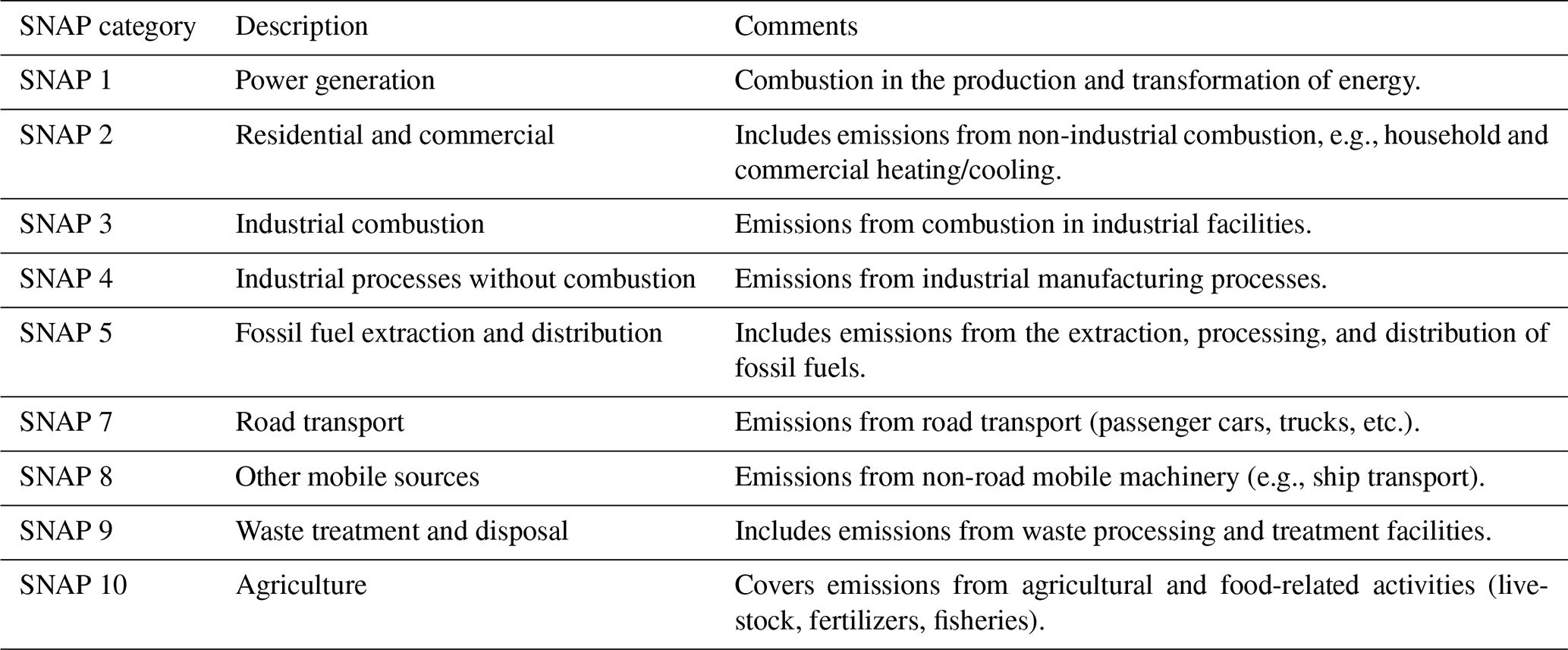
We differentiate between two types of anthropogenic emissions: point sources and spatially allocated diffuse sources, which are processed in separate procedures, as explained below.
Point sources, which include emissions from power plants and industrial facilities, are the largest contributors to the anthropogenic CO2 budget, accounting for approximately 50 %–60 % of total anthropogenic CO2 emissions. In the Netherlands, companies responsible for these large emission sources are required to report emissions annually by location to a pollutant register. Reported emissions from these sources are available on the National Emission Inventory (ER) portal, maintained by RIVM (https://data.emissieregistratie.nl/export, last access: 27 November 2024, hereafter referred to as the ER portal). This portal provides an annual total emission inventory database of GHGs as well as other specific variables relevant to air quality.
Emission data are classified by sector/subsector, facilitating processing for each SNAP category. Emissions from industrial point sources are accessible through the ER portal, aggregated at the company level. A comprehensive list of registered emission sources, including thermal plume parameters such as exhaust temperatures and volumetric flow rates, as well as the stack height of the emission itself, can be obtained from the RIVM upon request.
Aside from this, gridded CO2 emissions with a spatial resolution of 1 × 1 km2 over land and 5 × 5 km2 over the North Sea are also available from the ER portal. The 1 × 1 km2 spatial resolution cannot be easily refined for all emission sources due to various reasons; for some emissions there is a lack of suitable data to do so, and sometimes privacy protection rules play a role. For most emission sources, spatial allocation is done by applying an allocation key dataset; e.g. all emissions related to citizens are commonly gridded based on the population number. Some total emissions are estimated using calculation methods in which spatial data are implemented/available (e.g. Automatic Identification System (AIS) data of ship movements); in this case, only aggregation to the desired spatial scale is needed. For industrial sources, stack coordinates are registered through industrial activity surveys related to the European Pollutant Release and Transfer Register regulation. An uncertainty of approximately 4 % is reported for the total CO2 emissions in the emission inventory.
Comprehensive information on the methods used for the production and processing of the emission inventory, as well as uncertainties for different sectors, is provided in the National Inventory Report (Van der Net et al., 2024).
The Dutch Atmospheric Large-Eddy-Simulation (DALES) model is a community-based numerical framework designed for atmospheric research, which focuses in particular on small-scale atmospheric turbulence processes including clouds and the physics of the ABL (Heus et al., 2010; Ouwersloot et al., 2017). DALES originates from the code developed by Nieuwstadt and Brost (1986). In this work, we use DALES version 4.4, which can be accessed here: Karagodin-Doyennel (2024a).
DALES is based on LES techniques, which resolve eddies in turbulent flow down to a certain scale (typically the size of the grid cells), below which small-scale turbulent structures are parameterized. Therefore, no parameterization of processes such as ABL entrainment or plume mixing is required (Dosio et al., 2003). In addition, DALES incorporates state-of-the-art atmospheric physics and microphysics schemes to simulate various processes, including radiation, convection, and cloud formation. These components are crucial for accurately representing the exchange of momentum, heat, moisture, and other substances between the atmosphere and the Earth's surface.
DALES has been proven to accurately reproduce observed atmospheric turbulence and other dynamical processes, providing valuable insights into ABL phenomena, atmospheric dynamics, and cloud and aerosol microphysics (Sikma and Ouwersloot, 2015; de Bruine et al., 2019). DALES is formulated on a rectilinear x–y grid and configured to use the Arakawa C grid (Arakawa et al., 2011, 2016). For this setup, Lambert Conformal Conic (LCC) coordinates are employed in DALES. Tracer advection is simulated using the Kappa mass-conserving scheme (Tatsumi et al., 1995). The Kappa scheme is a hybrid advection scheme that combines aspects of first-order upwind schemes and second-order centered schemes for parameters such as tracer mixing ratios that should never become negative. The filtered Navier–Stokes equations are solved on the DALES grid, allowing extremely fine spatial resolutions (up to 1 m) horizontally and from a few meters to several hundred meters vertically using a stretched vertical grid. DALES has been developed for the troposphere; therefore, the vertical grid begins at ground level and can be extended up to a height of about 11 km. DALES employs a temporal integration time as fine as 2 s.
DALES features an interactive land surface simulation, including photosynthesis as well as soil and autotrophic respiration, using the Land Surface Model (LSM) (Jacobs and de Bruin, 1997; Ronda et al., 2001; Jacobs et al., 2007; Balsamo et al., 2009; Vilà-Guerau de Arellano et al., 2014). Involving the LSM is particularly valuable for studying the effects of land cover heterogeneity on atmospheric dynamics, microphysics, and ABL development, as well as atmospheric influences from the biosphere.
LSM provides DALES with the ability to compute net biogenic CO2 fluxes, such as biospheric sinks through vegetation photosynthesis and respiration fluxes. This is achieved in DALES using a dedicated scheme that integrates canopy and soil resistances based on the A-gs (net CO2 assimilation rate (A) and stomatal conductance (gs)) model. The performance of A-gs has previously been evaluated, showing results similar to those of the widely used Farquhar biochemical growth model (van Diepen et al., 2022). Initially proposed by Jacobs and de Bruin (1997) and later refined and simplified by Ronda et al. (2001), the A-gs scheme adopted by DALES enables the calculation of stomatal conductances for both CO2 and water, facilitating CO2 exchange between vegetation and the atmosphere. The transport of CO2 into the leaf is the result of gross assimilation and dark respiration. Autotrophic respiration is considered based on R10, which represents respiration at 10 °C (Jacobs et al., 2007). Hence, the scheme incorporates a parameterization for soil respiration of CO2 and the influence of soil moisture on canopy conductance.
Ultimately, the scheme provides information on net CO2 assimilation (photosynthesis) and soil respiration, taking into account factors such as temperature and vegetation type. While the A-gs scheme in DALES is primarily focused on grassland ecosystems, this work enhances the scheme by incorporating parameters specific to forests. Parameters for the A-gs model used in DALES for both vegetation types are provided in Table A1, and the map distinguishing between regions with grassland and forest is shown in Fig. 1.
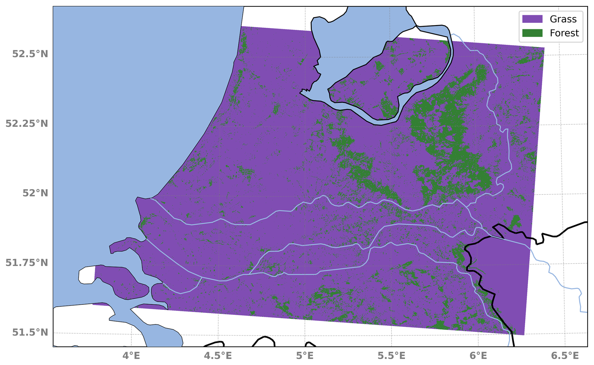
Figure 1Map of vegetation types used by the LSM in DALES. The map corresponds to the target LES domain (100×100 m) used in this study. The purple color represents grassland areas, and green represents forested areas.
Distinguishing between forest and grassland is particularly important in the central–eastern region of the Netherlands, where forests are prevalent. Large forested areas within urban areas are also considered. This distinction improves the accuracy of the computed CO2 and momentum fluxes due to forest-specific surface roughness.
3.1 DALES boundary conditions
In our work, several datasets are used for lateral and vertical boundary conditions for meteorology and chemistry. The meteorological lateral boundary conditions (LBCs) in DALES are nudged toward data from the HARMONIE-AROME mesoscale weather forecast model developed at the Royal Netherlands Meteorological Institute (KNMI; Bengtsson and Coauthors, 2017). To nudge DALES lateral boundaries toward HARMONIE-AROME, we use a distinct dataset from the Winds of the North Sea in 2050 (WINS50) project (see https://www.wins50.nl/, last access: 27 November 2024, for additional details), which provides coverage over the Netherlands at an hourly temporal resolution (see https://dataplatform.knmi.nl/dataset/wins50-wfp-nl-ts-singlepoint-3, last access: 27 November 2024, for further details). It uses common meteorological variables such as wind speed, wind direction, temperature, air pressure, relative humidity, and sea surface temperature.
To incorporate background CO2 concentrations, LBCs are applied based on the Copernicus Atmospheric Monitoring System (CAMS) air quality forecast of the CAMS Global Greenhouse Gas Reanalysis (EGG4) product. This product is based on the delayed-mode analysis, which provides a refined, post-processed dataset that offers a more accurate representation of greenhouse gases in the atmosphere. We use these data for a geographical area spanning 50.5 to 54.0° N and 1.75 to 9.125° E at a resolution of 0.125° × 0.125° (∼ 14 km), updating them every 6 h (for further details on the CAMS EGG4 product, visit https://ads.atmosphere.copernicus.eu/datasets/cams-global-ghg-reanalysis-egg4?tab=overview, last access: 11 March 2025).
LSM also requires initial state data for initialization, encompassing parameters such as land use; vegetation properties from ERA5 data; and soil hydraulic parameters for 42 soil types, including soil moisture content in different states, hydraulic conductivity at saturation, Van Genuchten model parameters used to describe soil water retention, and hydraulic properties (see Vilà-Guerau de Arellano et al., 2015).
Note that in this study, the DALES with periodic lateral boundaries is used. This periodicity applies to mean wind, turbulence, and tracers, meaning that any quantity exiting the eastern boundary re-enters at the western boundary and vice versa; the same applies to the north–south boundaries. The upper boundary incorporates a damping sponge layer that gradually reduces turbulence and tracers to minimize artificial reflections. At the bottom, surface heterogeneity affects the fluxes, which are treated by the LSM.
Overall, due to its accuracy, fine spatial and vertical resolution (100 m horizontal and 20 m within the ABL), and near-realistic modeling approach (including a heterogeneous surface, anthropogenic emissions, and periodic boundaries), DALES is well-suited to conduct targeted simulations that isolate and examine specific aspects of atmospheric physics and dynamics under controlled conditions. Since DALES had not previously been utilized for modeling CO2 mole fractions, coupling with an emission inventory required additional development to incorporate a program that converts and integrates emissions data for accurate horizontal representation, as well as for vertical allocation in the model.
To integrate and simulate the transport of anthropogenic emissions within DALES, we developed a module to read emission datasets, to apply vertical allocation of emissions and inter-hour interpolation to integrate a smooth change in emissions, and finally to apply emissions to scalar CO2 tracers. In the simulation setup used in this study, the scalar tracer for atmospheric transport of CO2 in DALES is expressed in units of µg g−1. The expression used to translate area emission profiles into model scalar tracers is as follows:
where CO2tracer is the scalar CO2 tracer [µg g−1], area_emis_int is the temporally interpolated 3D field of emission input [kg h−1], ρj is air density [kg m−3], dzfj is the thickness of the full level [m], dx and dy are grid spacing in x and y directions [m], is the conversion factor from kilograms to micrograms, j denotes the vertical layer index from 1 to kemis where emissions are allocated (for area emissions, and kemis equals the closest layer to 150 m according to the results of Brunner et al., 2019). It should be noted that since the emission input has an hourly temporal resolution, an inter-hour interpolation factor is calculated, and temporal linear interpolation of emissions is applied.
For area emissions, the representation of area emission plume rise is simplified by setting the plume bottom height to 0 and the plume top height to ∼ 150 m, following Brunner et al. (2019). Emissions are evenly distributed among model layers between the emission bottom and top heights, so each layer receives an equal share of the total emission values. It is important to note that area emissions from several SNAP categories have no vertical component, and all emissions from those categories are applied to the model at the lowest LES layer. These categories are SNAP 5 since oil/gas extraction occurs at ground level; SNAP 7 traffic emissions; and SNAP 10 agriculture since it involves emissions at the near-ground level, such as those from soil and livestock.
In the case of point sources, the plume bottom and emission altitude can be calculated interactively. The effective emission height can be significantly higher than the geometric height of a stack due to the buoyancy of the emission flux (Briggs, 1984). Therefore, plume rise is influenced by several factors, including stack geometry, flow properties (such as exhaust temperature and volumetric flow rate), and meteorological conditions (such as air temperature, wind speed, and atmospheric stability) (Brunner et al., 2019). To account for this in the simulation, the DALES emission module includes an online algorithm that calculates plume rise based on the interaction between the model meteorology and source-specific data at each model time step.
4.1 Online algorithm for calculating plume rise height
The algorithm implemented in DALES to calculate the plume height above the stack, as well as the vertical boundaries of the plume after it has risen to equilibrium, was originally proposed by Briggs (1984). We implemented a revised, up-to-date version of this algorithm, as outlined in Gordon et al. (2018) and Akingunola et al. (2018).
Initially, since the calculated stack height may not align exactly with a model grid point, the air temperature (Ta) and wind speed (Ua) at the stack height are determined from DALES data using linear interpolation. Once the atmospheric variables are obtained, the buoyancy flux (Fb) at the stack height, responsible for the updraft of turbulent eddies, is calculated based on the difference between the emission temperature (Ts) and Ta using Eq. (1) from Akingunola et al. (2018). This calculation indicates that the emitted plume is buoyant and rises only when Ts exceeds Ta. The plume parameters are assumed to be in steady-state conditions, as information about their temporal changes is unavailable.
Further, the residual buoyancy flux (F1) is estimated based on atmospheric conditions and emission characteristics. With an iterative process that continues until F1 becomes negative, we compute the local stability parameter (Sj) for each subsequent model level using Eq. (5) from Akingunola et al. (2018). Note that the iteration initializes at the stack height (hs).
is calculated sequentially for each atmospheric layer based on the value of S, selecting the final value that shows the greatest decrease in flux, as recommended by Briggs (1984), as follows:
where the mean wind speed Um is calculated as , as recommended by Gordon et al. (2018) (where U is , representing the total horizontal wind speed). In the first iteration, and . The stack height is subtracted from each z value, representing the vertical distance relative to the top of the stack. Initial values for F1 are set to .
Finally, the exact plume rise height (hmax) is determined based on the condition that at hmax equals 0, indicating that hmax is the altitude at which the buoyancy flux of the emitted plume dissipates entirely (Akingunola et al., 2018). Thus, the expression for hmax can be derived from Eq. (2) and and applied to the layer where becomes negative, as follows:
If , then hmax equals the altitude of .
Using the plume rise height hmax, the top (zt) and bottom (zb) of the plume are then calculated using Eq. (8) from Akingunola et al. (2018).
The illustration of the resulting plume top distributions for midday (12:00 UTC) and midnight (00:00 UTC) is depicted in Fig. 2.
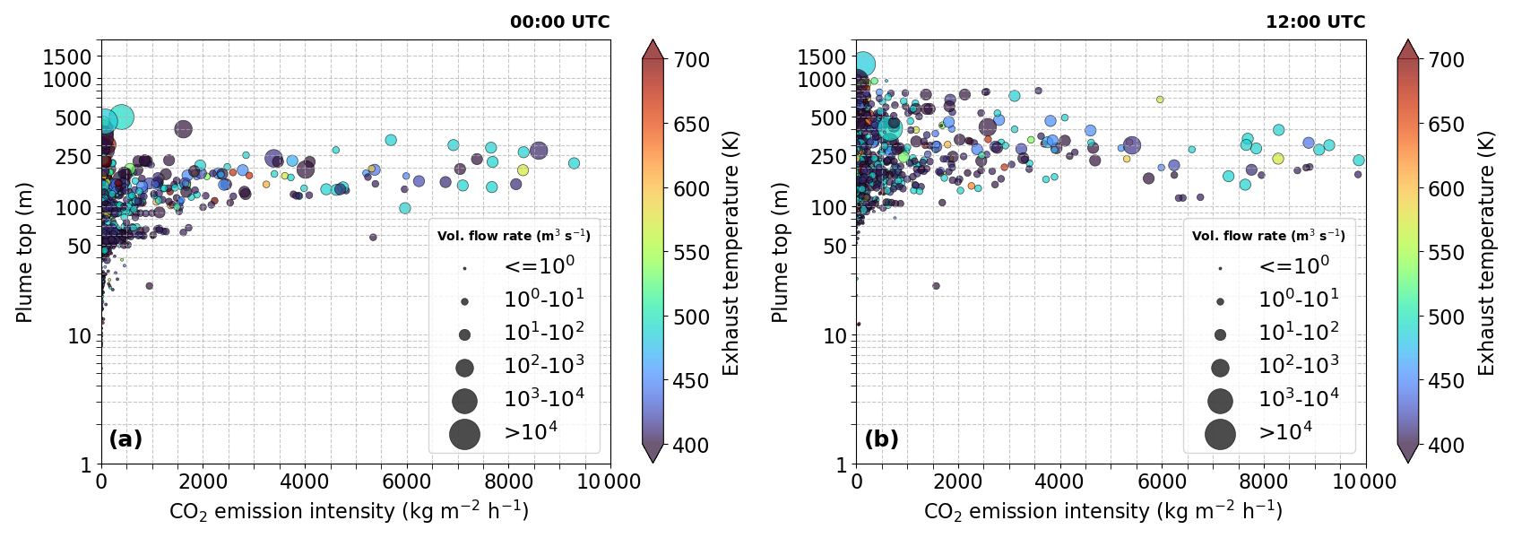
Figure 2Modeled plume top (zt) distribution as a function of the corresponding CO2 emission intensity (kg m−2 h−1) at (a) 00:00 UTC and (b) 12:00 UTC. Dot color: exhaust temperature (K); dot size: volumetric flow rate (m3 s−1).
Despite the exhaust temperature and volumetric flow rate remaining constant in the algorithm, a pronounced difference in plume top distributions between night (00:00 UTC) and day (12:00 UTC) is visible. This difference is primarily due to local atmospheric conditions. During the night (00:00 UTC), the plume tops are confined to below 500 m. In contrast, during the day (12:00 UTC), the plume tops exhibit greater variability, with some tops reaching up to 1500 m.
At night, the atmosphere is more stably stratified, with little turbulence and reduced vertical mixing. This stable stratification acts as a natural barrier, preventing plumes from rising higher into the atmosphere. Additionally, the boundary layer is lower at night, further constraining the height of plume rise. In contrast, during the daytime, solar heating causes surface warming, leading to increased atmospheric turbulence and stronger vertical mixing. This creates a deeper and more unstable boundary layer, spurring the plumes to rise higher. The convective upflow during the day enhances the buoyancy of plumes, contributing to the broader distribution of plume tops observed at 12:00 UTC. Hence, the difference in plume top heights between night and day is largely driven by variations in atmospheric stability, turbulence, and boundary layer dynamics.
It is important to note that as with area emissions, point source emissions are equally distributed in the vertical direction from plume bottom to plume top, with grid cells fully covered by the plume. However, since the parameterization provides the exact plume bottom and plume rise heights, these altitudes may fall between the edges of the model layers. The fractions of layers covered by the plume top and bottom are calculated.
To include the point source emission profile in the scalar CO2 tracer and account for the vertical allocation of emissions using the calculated plume vertical boundaries, we use a similar expression as in Eq. (1) but apply it separately to three cases: zb=zt, , and . Note that in the case of , the plume fraction factors are not applied, and the total emissions are divided by 2 and equally distributed.
Thus, the use of the plume rise algorithm ensures a more accurate representation of CO2 plume vertical distribution, contributing to a more realistic dispersion of pollutants. The plume rise height is strongly influenced by turbulent conditions and variations in buoyancy flux (see Fig. 2), which are calculated based on the differences between plume thermal parameters, ambient meteorology, and atmospheric stratification and stability.
It should be mentioned that the emissions from the point and area sources utilized in our study represent the total national annual emissions, which are quantified in kilograms of CO2 per year. Thus, these data need to be spatially and temporally disaggregated before being used as input for DALES. This is achieved through a downscaling workflow procedure, which is described in the following section.
Coupling the CO2 emission inventory with a high-resolution model like DALES requires alignment between the spatiotemporal resolutions and coordinate systems of the emission inventory and the model. In this study, DALES input uses a LES grid with a 100 m horizontal resolution and emission input with an hourly temporal resolution to account for the diurnal variations. Therefore, to accurately simulate CO2 emissions, the emission data must be disaggregated in both space and time.
Consequently, a translation of the coordinate system to LCC coordinates is required, as the original emission datasets from the national registry are provided in Dutch Rijksdriehoek (RD) coordinates. Thus, we developed a downscaling workflow to convert the prior emission inventory into DALES-compatible input.
The workflow is structured as a comprehensive program with several stand-alone modules, each responsible for different aspects of emission data processing. The full description of the program and all modules included can be accessed in Karagodin-Doyennel (2024b). Since DALES computes point sources and area emissions differently, the model input is separated into these two components. Initially, the workflow focuses on preparing point source data for DALES (in point_source_explicit_input_netcdf.py). For individual sources with precise emission locations, emissions are straightforwardly reassigned from RD to LCC coordinates. Since DALES also calculates plume rise and emission altitudes interactively for point sources (as was discussed in Sect. 4.1), additional information on chimney height, exhaust temperature, and volumetric flux is required to calculate plume rise and the plume vertical borders between which CO2 is injected into the model atmosphere.
Unfortunately, not all point sources contain complete data. For instance, in the emission inventory for the year 2018, ∼ 68 % of point sources had gaps in data, such as missing the exhaust temperature, volumetric flow rate, or stack height. In this case, a gap-filling approach is employed for point sources using ordinary linear regression based on emission categories. This applies polynomial regression models to estimate missing or zero values in plume characteristics based on the logarithm of emission values. For volumetric flow rate and stack height, linear regression models of polynomial order 1 are applied, with a logarithmic transformation for both. Temperature, which depends mainly on the emission process, uses a constant regression model (polynomial order 0), as it remains relatively stable across emission rates. Figure 3 represents the results of the gap-filling procedure. Thus, the program returns the predicted values for the missing entries. Note that point sources with incomplete data available for the regression are incorporated into area emissions.
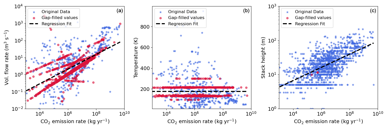
Figure 3Scatter plots of three plume parameters: volume flow rate (a), temperature (b), and stack height (c) as a function of the emission rate (kg yr−1). Each subplot combines the original data (blue stars) with the gap-filled values (red circles). A regression fit represents the overall dependence across the dataset.
Since the original emission data represent annual sums, temporal disaggregation down to the hourly level is required. For this, we applied Emissions Database for Global Atmospheric Research (EDGAR) temporal profiles for anthropogenic emissions specified by SNAP category (TNO, 2011; Crippa et al., 2020). This accounts for emission variations at daily, weekly, and monthly timescales, capturing variations such as traffic rush-hour patterns, seasonal differences in heating needs for households, and specifics for different countries.
Unlike point source emission processing, the workflow procedure to prepare a high-resolution-area emission inventory involves a more complex approach, as the exact coordinates of emissions are unknown. Initially, all point source emissions are subtracted from the area emissions, yielding residual area emissions (in ruisdael_area_residuals.py). Originally, in the national emission inventory, area emissions include contributions from both diffuse sources (e.g., transportation, residential heating, agriculture) and point sources (e.g., industrial facilities, power plants). However, since we process point source and area emissions separately, it is essential to remove the point source contributions from the area emissions to avoid double counting.
Subsequently, these residual area emissions are translated into GeoPackage (gpkg) format (in ruisdael_area_csv2gpkg.py ), which is an open, standards-based format for geospatial data storage. This format is chosen for its ability to precisely define spatial extent and select relevant subdomains within the Netherlands for simulation purposes. This eliminates the need for additional software (e.g., QGIS), reducing manual intervention.
The most computationally demanding operation in the workflow is the reprojection of area emissions to a high-resolution grid and from RD coordinates to the target LCC coordinates (in ruisdael_area_RD2HARM.py). The program matches the RD grid cells to the LCC coordinates and reassigns emissions to the new grid based on the proportional overlap of the grid box fractions. The emissions are then aggregated at the target resolution according to these proportions. This method is exact and is scale independent.
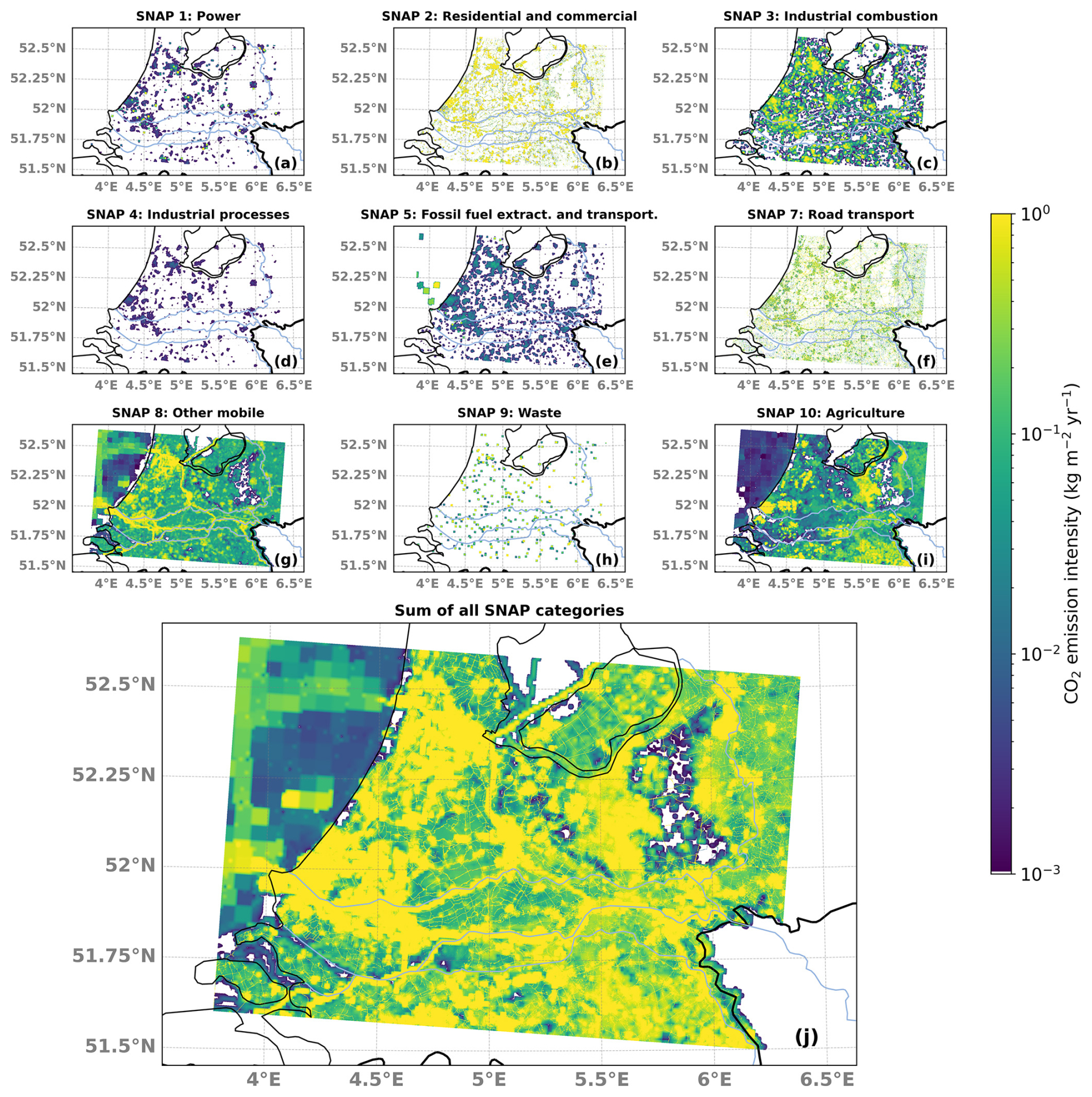
Figure 4Annual surface CO2 emission inventory (kg yr−1) over the target LES simulation domain (51.5–52.5° N, 3.75–6.45° E; resolution of 100 m) for the year 2018 categorized by SNAPs: (a) SNAP 1: power; (b) SNAP 2: residential and commercial; (c) SNAP 3: industrial combustion; (d) SNAP 4: industrial processes; (e) SNAP 5: fossil fuel extraction and transportation; (f) SNAP 7: road transport; (g) SNAP 8: other mobile; (h) SNAP 9: waste; and (i) SNAP 10: agriculture. Panel (j) is the aggregated CO2 emissions across all SNAP categories. These emission maps aggregate both area and point source emissions.
In Fig. 4, we show the contributions of different sectors to the total CO2 emissions, as well as the overall CO2 emissions from all SNAP categories combined. It is important to mention here that the current simulation setup has no sectorial split, and DALES uses combined emissions input from all SNAP categories. Over the sea, the resolution of the input emissions is much coarser (5×5 km2) than over the land (1×1 km2), as evidenced by the large squares over the North Sea. Marine emissions are included in the SNAP 8 category, representing ship traffic, as well as in SNAP 10, which accounts for fishery-related emissions, as they are more closely related to the food production sector than to transport activities. Although point sources are barely visible at a 100 m resolution (see Fig. 4j for more details), we present a combined view of area and point sources to provide a complete picture of emissions to verify the annual total within the selected domain. It is important to mention that the Rotterdam harbor, including its port infrastructure, and the Amsterdam area, together with the IJmuiden port, have the highest density of point source emissions within the simulation domain. The majority of point sources fall into the SNAP 1 (power generation) and SNAP 3 (industrial combustion) categories, as these sectors rely on large stationary facilities such as power plants, refineries, and industrial manufacturing sites. The point source/area emission contribution ratio to the total CO2 emissions in the simulation domain is ∼ 55 %45 %, with point sources having the higher contribution, as expected. The total sum of these emissions is approximately 109 Mt yr−1 for the selected domain, which aligns well with publicly available CO2 emission estimates for the Netherlands in 2018 (Ruyssenaars et al., 2021; https://ourworldindata.org/co2/country/netherlands?country=~NLD, last access: 27 November 2024). Since LESs are computationally expensive, the simulation domain only covers a part of the Netherlands. The selected domain includes the main focus area of the Ruisdael Observatory project (central part of the Netherlands), which is the most urbanized area of the country, responsible for the majority of carbon emissions (∼ 70 % of total national emissions). This ensures that all major CO2 sources in the region are included in the domain. To minimize the influence of CO2 surface fluxes and emissions from outside the Netherlands, aside from selecting a specific simulation domain, weather conditions with a stable northeasterly wind were selected for model evaluation (see Sect. 7.1). This minimizes the effect of CO2 emissions from Germany, which are not considered, as seen in the lower-right corner of the domain. Having the Groningen gas production area outside the simulation domain may omit its CO2 contribution due to the wind direction, but this impact is expected to be minimal due to the low GHG emission intensity of Dutch gas production. However, it should be noted that emissions outside the domain are accounted for in the CAMS EGG4 dataset. Further, the vertical distribution of area emissions is accounted for (as described in Sect. 4).
Finally, annual emissions are disaggregated down to the hourly level using the EDGAR temporal profiles, as discussed above for point sources (in create_hourly_emissions_3D.py). Note that the temporal integration time of DALES is approximately 2 s, so further inter-hour linear interpolation of emission input to smooth the hour-to-hour changes is necessary and is applied directly to the model code (see Sect. 4). The final input files are date specific and cover the complete simulation domain.
Figure 4 demonstrates the application of refinement methods using proxy or activity data for certain emission categories, which are explained further.
5.1 Refinement of area emissions: spatial disaggregation procedure
A spatial disaggregation procedure has been developed to refine CO2 emissions for relevant categories using several high-detail-activity-data proxies where such proxy data are applicable. The importance of the refinement procedure lies in its ability to enhance the accuracy and specificity of emission locations. In the current version of the workflow, proxy data for the residential and traffic emission categories are applied. To refine residential emissions from the residential combustion (SNAP 2) category, we employ demographic data from the Central Bureau of Statistics (CBS)1. These datasets provide statistical information on a large number of parameters, including demographics, gas/electricity use, housing, and energy for each 100 × 100 m2 square across the Netherlands.
To refine area emissions from the SNAP 2 category, we use information about the average annual consumption of natural gas or the total population density if gas usage is unknown. To refine the road transport (SNAP 7) category, we use a road shapefile that contains detailed data on traffic intensity and nitrogen oxide (NOx) emissions at the road level. This shapefile includes attributes such as the length of each road segment and NOx emission intensities from light, medium, and heavy vehicles. These attributes provide essential information on emission intensity across different road segments. We utilize the combined NOx emissions from these three vehicle types to determine the spatial distribution of traffic emission intensities within grids to derive CO2 emission weights for road segments relative to traffic intensity. Thus, using these weights enables the refinement of CO2 emissions from a 1×1 km2 resolution to the target level (100 m). The annual NOx emission traffic shapefile can be accessed from the Zenodo repository (Doyennel, 2025, https://doi.org/10.5281/zenodo.14961517).
The refinement process for both SNAP 2 (residential and commercial) and SNAP 7 (traffic) is illustrated in Fig. 5.
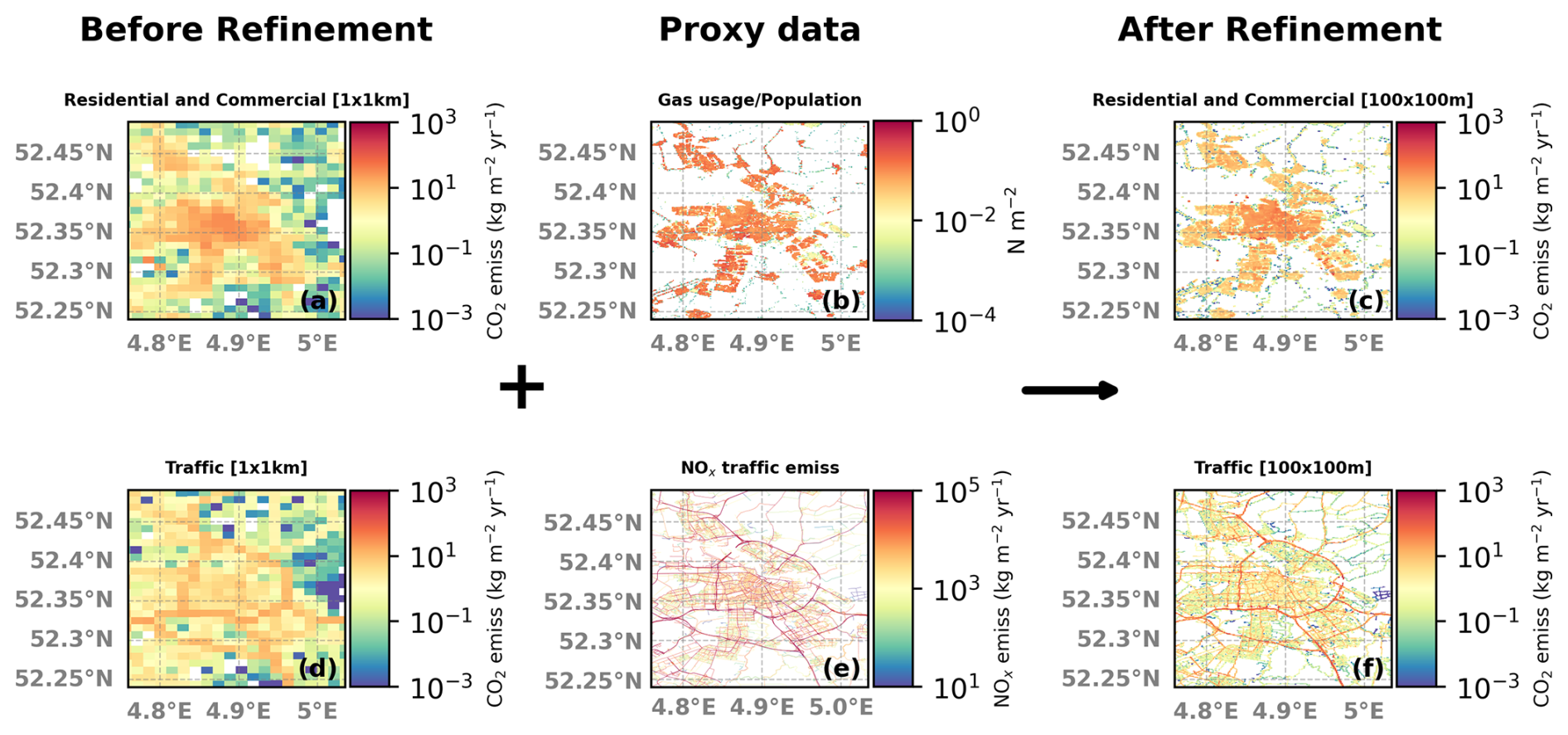
Figure 5Illustration of the spatial redistribution of annual CO2 area emissions (kg m−2 yr−1) from a coarse resolution of 1×1 km2 to a finer resolution of 100×100 m2, which is suitable for DALES, made for two SNAP categories: residential combustion (SNAP 2) and road transport (SNAP 7). This illustration focuses on the area surrounding the city of Amsterdam. (a, d) CO2 emission fields (kg m−2 yr−1) at the coarse resolution (1×1 km2); (b): the gas usage/population density (N m−2); (e): aggregate NOx emission data (kg m−2 yr−1) from three vehicle types: small, medium, and heavy; and (c, f) the resulting refined CO2 emission fields (kg m−2 yr−1) at a fine resolution (100×100 m2).
Figure 5 demonstrates that spatial information gained in the emission disaggregation process substantially improves the representation of emissions at the hectometer resolution required in the DALES numerical experiments. Without refinement, downscaling from a 1 km to a 100 m resolution would inaccurately retain 1 km shapes of objects, misallocating emissions. Using proxy data such as NOx emissions and household statistics further enhance the fidelity of emission downscaling, making estimates more spatially accurate when representing real-world conditions.
6.1 Systematic experiments for CO2
To assess the contributions of different sources to the overall CO2 concentration based on their origin, we devised a comprehensive model experiment featuring four distinct passive scalar CO2 tracers with the following setups:
-
CO2bg. This represents the background concentration derived from CAMS.
-
CO2bg_emiss. This combines the background concentration with all anthropogenic emissions.
-
CO2bg_emiss_resp. This combines the background concentration, anthropogenic emissions, and net soil respiration.
-
CO2sum. This combines all contributions to atmospheric CO2 included in DALES: CO2bg, CO2emiss, CO2resp, and the net CO2 assimilation (CO2photo).
The CO2bg tracer uses CO2 molar fractions from CAMS reprojected onto the DALES domain boundaries. CO2sum in DALES is the final CO2 tracer, which can be compared to observations, as it includes all considered components of atmospheric CO2 variability. Note that LSM uses the CO2sum tracer to calculate the ambient CO2 mixing ratio.
The impact of photosynthesis can be isolated by subtracting CO2bg_emiss_resp from CO2sum due to the linearity of passive tracer transport in DALES. This experimental setup allows the anthropogenic and biogenic components of CO2 variability to be derived and evaluated separately. Note that the current implementation does not include a sectoral split; however, this can be easily adjusted to analyze the contributions of specific sources.
As mentioned above, in this experiment DALES is configured with the simulation domain spanning 51.5 to 52.6° N and 3.75 to 6.45° E, with a horizontal resolution of 100 m (see Sect. 5). The vertical resolution ranges from approximately 25 m (within the ABL) to a few hundred meters. This is due to the use of a stretched vertical grid with 128 layers, an initial layer thickness of 25 m (dz0=25), and a stretching factor of 0.017 (α=0.017) that causes the layer thickness to increase geometrically with height.
6.2 Selected period of simulation
We assess the ability of DALES to simulate daytime CO2 variability during the summer period from 25 to 28 June 2018. The selection was made based on the availability of model input data (particularly regarding nudging large-scale meteorology) and the CO2 measurements for validation.
The period was characterized by stable summer conditions with predominantly clear skies and relatively warm temperatures. Winds were light to moderate, with a prevailing northeasterly flow (see Fig. 6) contributing to weak atmospheric mixing during the late-evening and early-morning hours. These meteorological conditions were ideal for evaluating CO2 variability and facilitated the detection of both anthropogenic emissions and biogenic contributions to the CO2 mole fractions.
To ensure model stability, several periods affected by the initialization spin-up were disregarded. DALES initialization typically occurs during the first 4 h of the simulation, when the fields evolve from small turbulent motions to fully turbulent conditions, with radiative transfer initialized, as suggested by Savazzi et al. (2024). We also excluded the times corresponding to the initialization of the HARMONIE forecast, which occurs at the start of each simulation day. It is advisable to exclude the first 6 h (Fischereit et al., 2024). Furthermore, periods with a stable atmospheric boundary layer (SABL) were excluded from the analysis. An accurate representation of the nocturnal SABL in DALES would require an increase in resolution from 100 to <10 m (Dai et al., 2021; Umek et al., 2022), which is not feasible given the domain size and setup used in this study. Thus, the period from 23:00 to 06:00 UTC each day that covers all the limitations mentioned was excluded from the analysis. This approach ensures that biases related to model initialization and known limitations are significantly mitigated.
7.1 In situ observations
To evaluate and validate the modeling framework developed, we use data from several measurement sites across the Netherlands (see Fig. 6).
We use hourly averaged in situ measurements of near-surface atmospheric CO2 concentrations around the city of Rotterdam that were made at two urban background stations, which are part of the Dutch Ruisdael Observatory, located at Westmaas (51.786° N, 4.45° E; sampling height is 10 m) and Slufter (51.933° N, 3.999° E; sampling height is 10 m), near the shore of the North Sea (see Fig. 6). Aside from this, the longest measurement time series is from the Cabauw tower (51.9703° N, 4.9264° E). The Cabauw Atmospheric Observatory measures atmospheric CO2 concentrations at four distinct elevations: at 27, 67, 127, and 207 m above the ground. These measurements are essential for a comprehensive characterization of local vertical gradients of CO2 within the lower ABL, enabling a detailed investigation into the vertical distribution of and temporal variability in GHGs. The hourly averaged CO2 mole fraction data from Cabauw (Hazan et al., 2016) are freely available from the ICOS Carbon Portal (https://data.icos-cp.eu/portal/, last access: 27 November 2024) for both ICOS and non-/pre-ICOS periods (Frumau et al., 2024a, b, c, d). These locations allow us to test and assess the model performance for the different contributions to CO2. Slufter is located on the 2e Maasvlakte, close to the shore of the North Sea, while Westmaas is south of Rotterdam in an agricultural area. The dominant wind direction in the Netherlands is from the southwest, so on many occasions, both stations are upwind of the industrial–urban complex of the Rotterdam Rijnmond area. However, during the simulated period, the average wind direction was from the northeast (see Fig. 6), and Westmaas is located downwind of Rotterdam. The Cabauw tower is situated in a rural area with a mixed contribution of vegetation (generally grassland) and dispersed anthropogenic emissions originating from either dispersed local-area sources or distant urban areas.
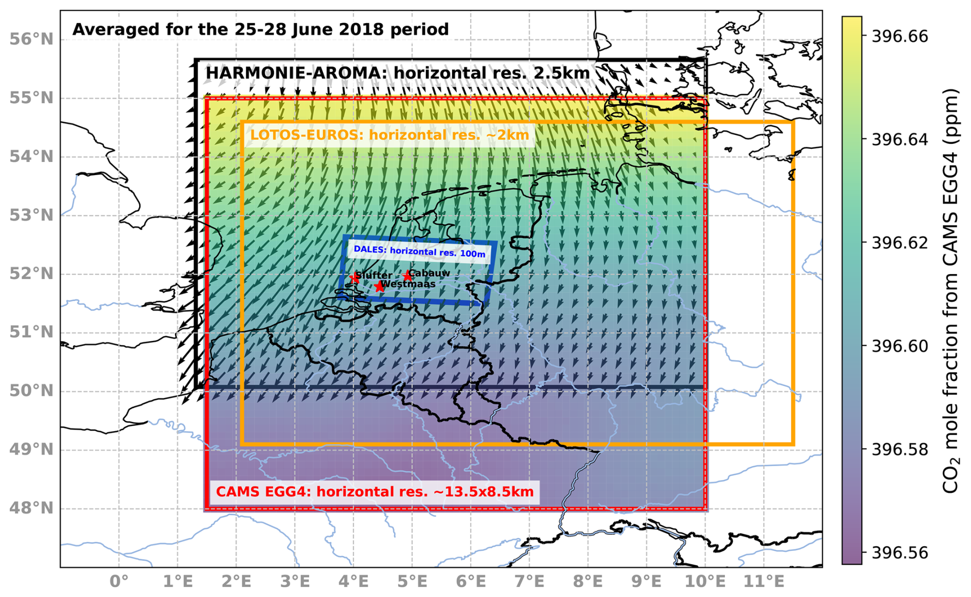
Figure 6A map of the Netherlands with the measurement sites used to assess the simulations of atmospheric CO2. The map shows surface CO2 mole fractions from CAMS averaged over 25–28 June 2018. Red stars indicate measurement locations from left to right: Slufter (51.933° N, 3.999° E), Westmaas (51.786° N, 4.45° E), and the Cabauw tower (51.9703° N, 4.9264° E). The blue dashed line represents the borders of the DALES domain. The orange rectangle represents the borders of the LOTOS-EUROS domain. The black rectangle represents the borders of the HARMONIE-AROMA domain. The arrows indicate the wind direction averaged over 25–28 June 2018. The length of the arrows represents the wind speed.
7.2 LOTOS-EUROS simulation
The LOTOS-EUROS chemistry–transport model is used in comparison to DALES to assess the added value of using a high-resolution turbulence-resolving model to simulate the observed variability in atmospheric CO2 in the Randstad area. LOTOS-EUROS is a state-of-the-art regional-scale community model developed jointly by TNO (the Netherlands Organisation for Applied Scientific Research) and RIVM (Schaap et al., 2008; Manders et al., 2017) and is designed to simulate the dispersion and transformation of air pollutants in the atmosphere, including aerosols, ozone, and trace gases. It accounts for anthropogenic and biogenic emissions, using complex chemical and physical processes for detailed forecasts of air quality and trace gas concentrations. The model links emission sources to atmospheric processes and transport, offering a comprehensive view of pollutant behavior and distribution (for more information about LOTOS-EUROS, visit https://airqualitymodeling.tno.nl/lotos-euros/, last access: 27 November 2024).
For our study, LOTOS-EUROS was employed to model CO2 variability with a finer resolution than its standard configuration. Although the standard resolutions of LOTOS-EUROS are approximately 7–25 km2, the simulations used in this work were performed at a horizontal resolution of ∼ 2 km. Turbulence is parameterized in LOTOS-EUROS, enabling us to evaluate the benefits of using explicit turbulence in comparison with DALES. While the vertical resolution of LOTOS-EUROS is similar to that of DALES (∼ 20 m within the ABL), terrain-following vertical layers are used in LOTOS-EUROS, whereas in DALES, the surface is assumed to be flat to simplify the turbulence, and thus topographical variations are not explicitly accounted for. However, for the majority of the Netherlands, the effect of topography is rather small. The CO2 setup of LOTOS-EUROS uses emissions from the CoCO2 project (https://coco2-project.eu/, last access: 27 November 2024) that are similar to those of DALES, except for the high-resolution emission disaggregation explained earlier in this section. It should be noted that, contrary to in DALES, biogenic CO2 fluxes in LOTOS-EUROS are not simulated internally but are handled instead using external datasets. In the CoCO2 project setup, biogenic fluxes from the VPRM (Vegetation Photosynthesis and Respiration Model) dataset provided by DLR (Deutsches Zentrum für Luft- und Raumfahrt, the German Aerospace Center) are used as offline input in LOTOS-EUROS (Denier van der Gon et al., 2021).
7.3 Evaluation methods
To evaluate the model performance against observations, we employed a comprehensive statistical analysis that incorporates multiple performance metrics. We used linear regressions and the R2 coefficient to assess the relationship between modeled and observed CO2 mole fractions, quantifying the proportion of variance explained by the model. The R2 was calculated using the Python statistics package sklearn.metrics.
Additionally, we utilized the Taylor diagram, which includes metrics such as the normalized standard deviation, correlation, and root-mean-square difference (RMSD), to evaluate the model's ability to reproduce observed variability. Furthermore, we calculate the mean bias error (MBE) and the root-mean-square error (RMSE) to quantify systematic deviations and overall discrepancies, respectively. MBE was computed as the average difference between the modeled and observed values, while RMSE was calculated using sklearn.metrics. In addition, a bootstrap analysis of the mean absolute error (MAE) was done to assess the significance of the differences between DALES/LOTOS-EUROS and observations with regard to MAE since the MAE estimate itself has uncertainty. This involves resampling observed and modeled data with replacement multiple times to generate different subsets.
These statistical methods allowed for a comprehensive evaluation of the model performance at replicating observed CO2 concentrations at various altitudes.
8.1 Comparison of simulation results
Figure 7 shows near-surface hourly averaged CO2 measured in parts per million (ppm) from DALES (upper panel) and LOTOS-EUROS (lower panel) for different times (06:00, 10:00, 16:00, 22:00 UTC) on 26 June 2018. As expected, DALES shows a more detailed representation of CO2 sources and their transport across the region than LOTOS-EUROS does. In the morning hours (06:00 UTC; Fig. 7a), elevated mole fractions are observed along the main roads, which are caused by increased traffic emissions during the morning rush hours, as well as in urban and industrial areas. The latter show up as bright plumes of elevated CO2. This is due to the combination of stable thermodynamic conditions and shallow boundary layers. The southwestern part of the region shows a noticeable intensification of CO2, likely due to point source industrial emissions, which dominate over other emission sources. Although LOTOS-EUROS reflects these emissions well, they appear to be more dispersed, with less recognizable differences between source types. Furthermore, LOTOS-EUROS shows slightly higher near-surface CO2 (up to 10 ppm more) than DALES does around urban areas at 06:00 UTC. This might be explained by less vertical mixing in LOTOS-EUROS than in DALES at this height and the absence of a vertical component of emissions in LOTOS-EUROS.
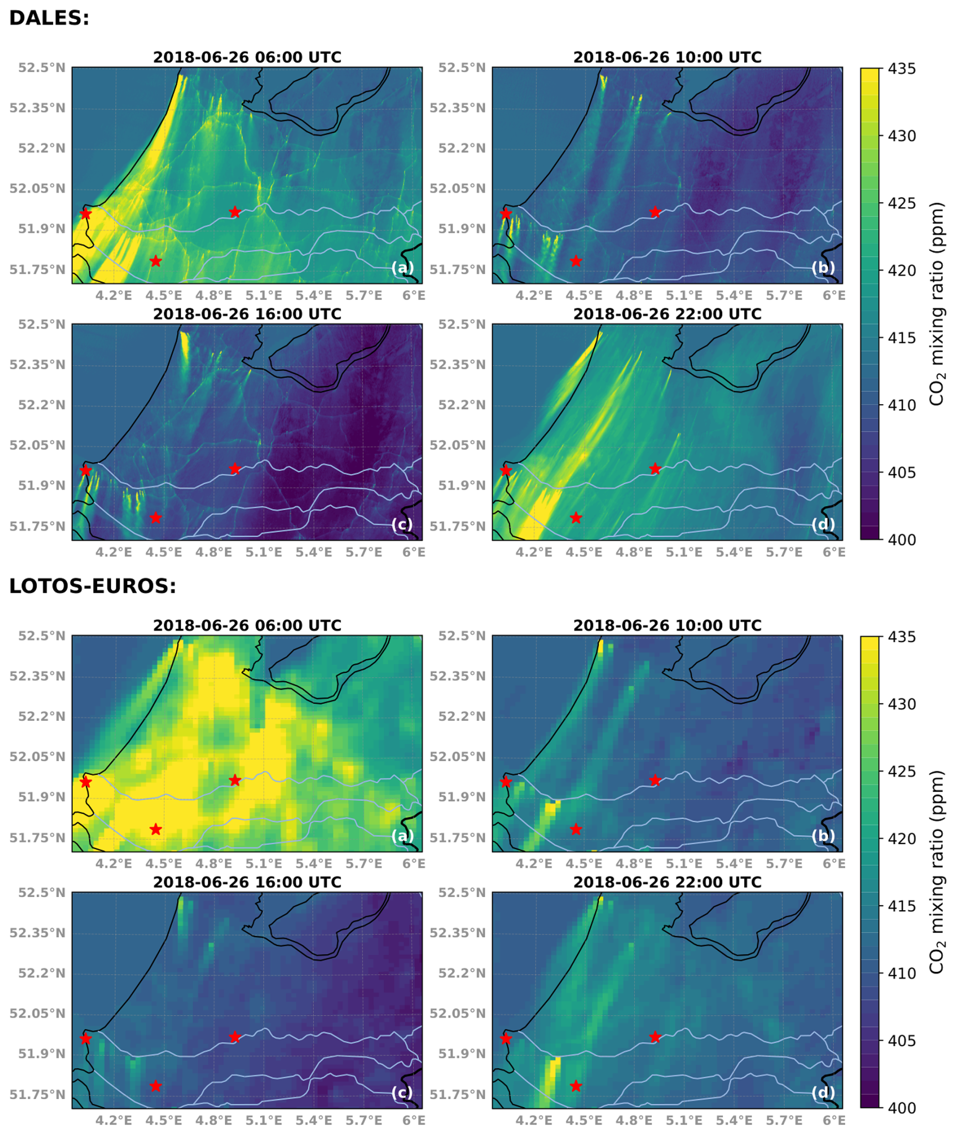
Figure 7Simulated near-surface (12.5 m height) hourly averaged CO2 mole fraction (ppm) for different times during the day on 26 June 2018 (in UTC for the end of the averaging period). (a) 06:00 UTC, (b) 10:00 UTC, (c) 16:00 UTC, and (d) 22:00 UTC. The domain covers the region from approximately 51.7 to 52.35° N and 4.0 to 6.0° E. Red stars mark the measurement sites from left to right: Slufter, Westmaas, and Cabauw tower (see Fig. 6). Upper panel: DALES at a 100 m horizontal resolution; lower panel: LOTOS-EUROS at a ∼ 2 km horizontal resolution.
At local noon (10:00 UTC; Fig. 7b), both models show a reduction in the CO2 mole fraction across urban areas and emission plumes, consistent with enhanced atmospheric mixing as the boundary layer thickness increases. The CO2 decrease of about 5–10 ppm over land is explained by biogenic CO2 uptake through photosynthesis. Both models show similar trends in this reduction, although variations in spatial detail remain.
In the late afternoon (16:00 UTC; Fig. 7c), there is greater spatial variability and a more pronounced decrease in background level, which is quite similar in both models (∼ 15 ppm), although the overall range of the CO2 molar fractions remains similar to those earlier in the day. DALES continues to show concentration signals that can more easily be attributed to local emissions, particularly along the transportation routes associated with the peak of traffic in the evening. LOTOS-EUROS captures these patterns but presents them in a more smoothed manner due to its coarser resolution.
Around local midnight (22:00 UTC; Fig. 7d), the simulated CO2 mole fraction distribution shows more stable conditions. Reduced atmospheric mixing at night leads to a higher CO2 mole fraction around urban areas. However, traffic emissions decrease considerably at this time, as expected. Both models reflect this nocturnal pattern, although LOTOS-EUROS continues to show higher near-surface concentrations during the night, although they are less pronounced than those seen in the morning hours.
Thus, diurnal variations in atmospheric CO2 near the ground are generally represented well in both models, reflecting changes in background, anthropogenic emissions, and biogenic activity under varying atmospheric conditions. DALES provides a more detailed representation of individual emission sources and spatial variability, while LOTOS-EUROS, due to its coarser resolution, does not resolve the different source types as well. However, before it can be concluded that DALES provides a more accurate representation of CO2, both models need to be compared to actual measurements, which we will turn to next.
8.2 The modeled CO2 against ground-based urban measurements in Westmaas and Slufter
The evaluation of modeled CO2 was conducted using ground-based urban measurements at the Westmaas and Slufter sites during the daytime hours from 25 to 28 June 2018. Here, for these time series, we show the deviation from the mean after subtracting the CO2 mean level over the period considered. This approach highlights the CO2 variability relative to a baseline, emphasizing deviations from average conditions. In addition, the time series of all anthropogenic emissions (AEs) and the net ecosystem exchange (NEE) influence on CO2 calculated from DALES have been added to show the local anthropogenic and biogenic contributions to CO2 overall variability separately. Since the measurements at Westmaas and Slufter were performed at one height (10 m), model data are interpolated horizontally to the exact latitude and longitude of the measurements, but vertically, the model data had to be extrapolated using the first two model layers since the lowest model layer is slightly above 10 m. The time series of CO2 mole fractions for the Westmaas and Slufter sites are presented in Fig. 8.
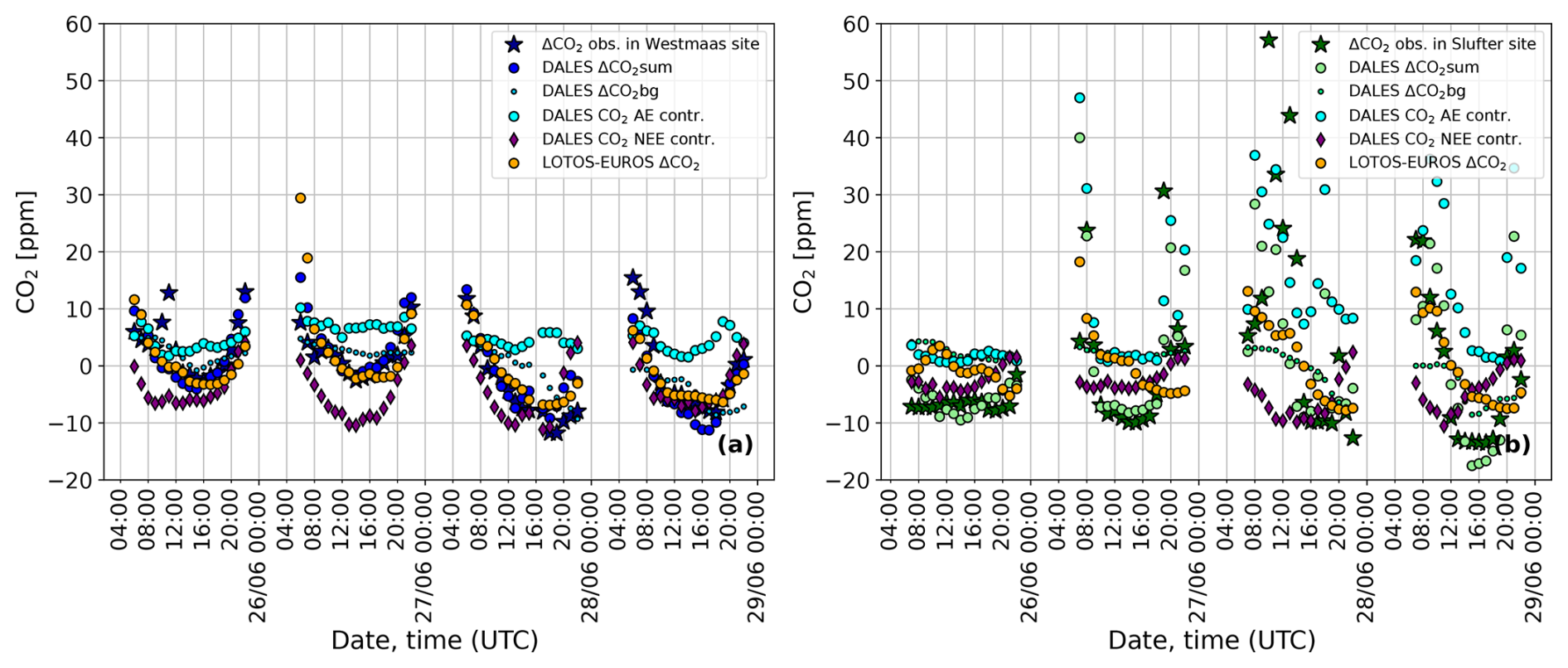
Figure 8Time series of the observed and modeled near-surface atmospheric CO2 mole fraction as a deviation from the mean from Westmaas and Slufter at a 10 m height for the period of 25–28 June 2018. (a) From Westmaas: observations (dark-blue stars) and model predictions (DALES CO2bg as light-blue dots, CO2sum as blue circles, AE contribution to the CO2 mole fraction from DALES as light-blue circles, the modeled NEE contribution to the CO2 mole fractions from DALES as purple diamonds, and LOTOS-EUROS CO2 in orange). (b) From Slufter: observations (dark-green stars) and model predictions (DALES CO2bg as light-green dots, CO2sum as light-green circles, AE contribution to the CO2 mole fraction from DALES as light-blue circles, the modeled NEE contribution to the CO2 mole fractions from DALES as purple diamonds, and LOTOS-EUROS CO2 in orange). All values presented are calculated relative to the CO2 mean by subtracting the mean value (the average CO2 mole fraction over selected times (07:00–22:00 UTC) during the 25–28 June 2018 period). The values are averaged hourly, with the time corresponding to the end of the averaging period.
At Westmaas (Fig. 8a), the observed near-surface CO2 (dark-blue stars) exhibits diurnal variability, with lower concentrations during the daytime due to vegetation uptake (reaching values below −10 ppm) and enhanced vertical mixing and higher concentrations in the early morning/late evening (10 to 15 ppm above the mean) due to stabilization of the ABL and soil respiration (NEE enhancement up to +5 ppm). The DALES CO2sum simulation (blue line) effectively captures the observed daytime declines, with a small (<2 ppm) discrepancy from the measurements. The local AE contribution (light-blue line in Fig. 8a) shows moderate variability throughout the period, fluctuating between 5 and 10 ppm. This is generally balanced by the CO2 NEE, leading to CO2sum having good agreement with observations for most of the period (see purple line). However, deviations of approximately ±5 ppm persist in the early morning/late evening, which may result from overestimations in vertical mixing or offsets in background concentrations, which can be up to 2.5 % (∼ 1 % on average) in recent years, as noted in Bennouna et al. (2024). In contrast, LOTOS-EUROS (orange line) tends to show larger deviations from the observations during these periods (by 3–5 ppm on average), although its general pattern follows the observations.
In contrast, at the Slufter site (Fig. 8b), both models exhibit greater disagreement with the observations (dark-green stars). However, DALES results indicate that the large variability observed is primarily due to the local AE contribution, which dominates CO2 variability at this location during 26–28 June, as seen from the large CO2 spikes (up to +60 ppm) (see Fig. 12b). This allows DALES CO2sum to better capture the daytime variability. The contribution of NEE also plays a role (up to −10 ppm), but its influence on CO2 variability is largely overshadowed by AE. The LOTOS-EUROS model (orange line) captures some of the observed variability, such as the late-evening fluctuations on 25 and 27 June, but fails to reproduce the finer-scale daytime spikes visible in the observations (see Fig. 12).
Note that the Slufter site presents additional challenges to the models due to its coastal location, where the interactions between land, sea, and atmospheric dynamics introduce complex and unique CO2 variability. These interactions, possibly involving sea breeze effects of temperature inversions, introduce fine-scale changes in CO2 levels that might be difficult to reproduce even with the current 100 m resolution DALES setup. DALES does show better daytime CO2 variability than LOTOS-EUROS does, pointing to the importance of local processes.
To further evaluate the simulation results, we performed a comprehensive statistical analysis using the methods described in Sect. 7.3. The results of the statistical analysis are presented in Fig. 9 and Table A2 in the Appendix. The results of the MAE bootstrap analysis are presented in Fig. B1.
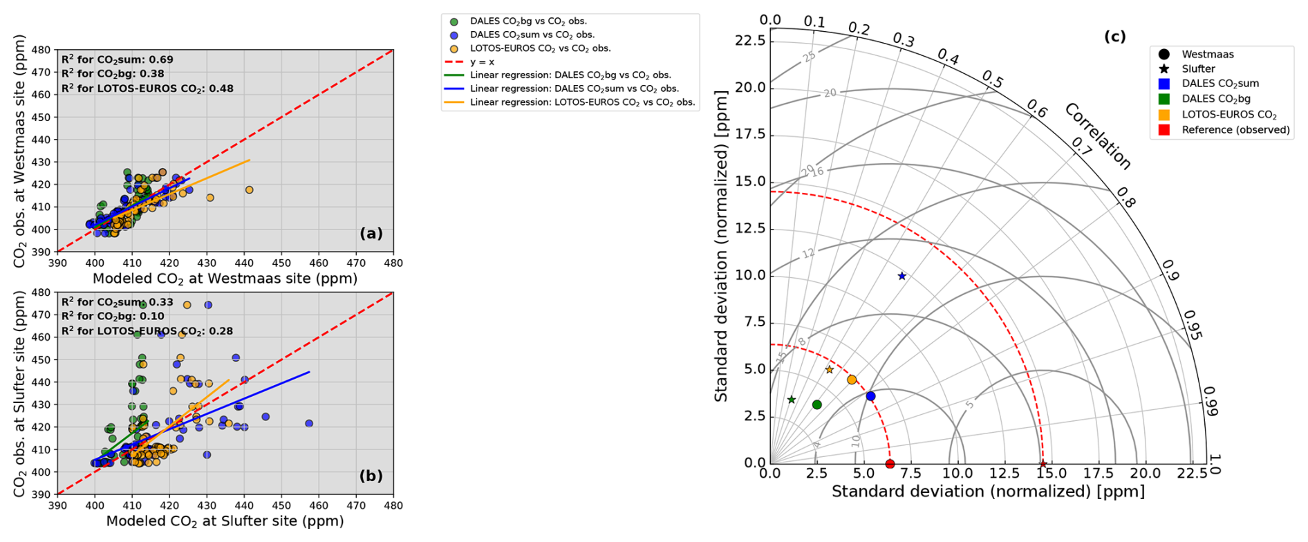
Figure 9(a, b) Density plot comparing model predictions (DALES CO2sum, CO2bg, and LOTOS-EUROS CO2) to observed CO2 concentrations for the daytime (07:00–22:00 UTC) during the 25–28 June 2018 period at Westmaas (a) and at Slufter (b). The red dashed line represents the ideal relationship (y=x line). Linear regression lines are shown for CO2bg (green), CO2sum (blue), and LOTOS-EUROS CO2 (orange), along with the corresponding regression equations and R2 values. (c) Taylor diagram quantifying the model performance against observations. Circle: Westmaas, star: Slufter. Blue: DALES CO2sum, green: DALES CO2bg, orange: LOTOS-EUROS CO2, and red: reference (observed CO2). Gray circular lines are the contours of equal RMSD.
In the urban background location of Westmaas (Fig. 9a), the regression analysis indicates a significant improvement in daytime CO2 variability prediction using DALES CO2sum compared to LOTOS-EUROS (R2: 0.69 vs. 0.48). This indicates that DALES CO2sum provides a more accurate representation of CO2 variability than LOTOS-EUROS does, particularly in capturing local-scale influences.
Furthermore, statistical metrics derived from the Taylor diagram also show an improvement in model predictions with DALES CO2sum compared to LOTOS-EUROS. This analysis shows a higher correlation (corr: 0.83 vs. 0.69), a normalized standard deviation closer to the observed value (SD: 6.46 vs. 6.25; observed SD: 6.38), and lower error metrics such as RMSD (RMSD: 3.76 vs. 4.93). Both MBE and RMSE are also lower for CO2sum than for LOTOS-EUROS (MBE: −0.19 vs. 1.97 and RMSE: 3.77 vs. 5.31), indicating lower overall errors and the highest accuracy of both variability and mean-level predictions in DALES at this location.
At the Slufter site (Fig. 9b), both models exhibit low R2 values (<0.5), indicating limited ability to explain observed variability. DALES CO2sum shows slightly better agreement with observations than LOTOS-EUROS does, with a higher R2 (0.33 vs. 0.28) and correlation coefficient (0.57 vs. 0.53). The high RMSD values for both models further indicate substantial deviations from observed concentrations, with LOTOS-EUROS showing a slightly lower RMSD (12.52 vs. 12.43). Similarly, the RMSE suggests a marginally lower total error in LOTOS-EUROS, while DALES provides a better estimate of the mean CO2 level (MBE: 0.15 vs. 0.39; RMSE: 12.52 vs. 12.44). Importantly, DALES captures the observed variability better, with a normalized standard deviation (12.23) much closer to the observed value (14.52) compared to LOTOS-EUROS (5.93), which means that DALES retains 85 % of observed variability, while LOTOS-EUROS captures only 40 %.
Overall, the results highlight the strengths and limitations of both models across different environments. At the urban background site of Westmaas, the representation of local-scale CO2 variability and mean-level accuracy is significantly improved in DALES, in particular due to the integration of highly resolved AE and NEE. However, despite some improvements in DALES, even with a high-resolution LES and detailed local sources, both models face comparable challenges when reproducing CO2 variability in the complex and dynamic coastal environment of Slufter.
8.3 The modeled CO2 against rural Cabauw tower observations
A similar analysis has been performed for the Cabauw tower location. The time series of the atmospheric CO2 mole fraction computed with DALES for the CO2bg and CO2sum tracers are compared to LOTOS-EUROS, as well as to the CO2 measurements from Cabauw tower presented in Fig. 10. To assess the ability of DALES to reproduce observed variability at various heights, modeling data that were sampled at the Cabauw tower were interpolated horizontally and vertically (using air density) to match the Cabauw measured CO2 profile.
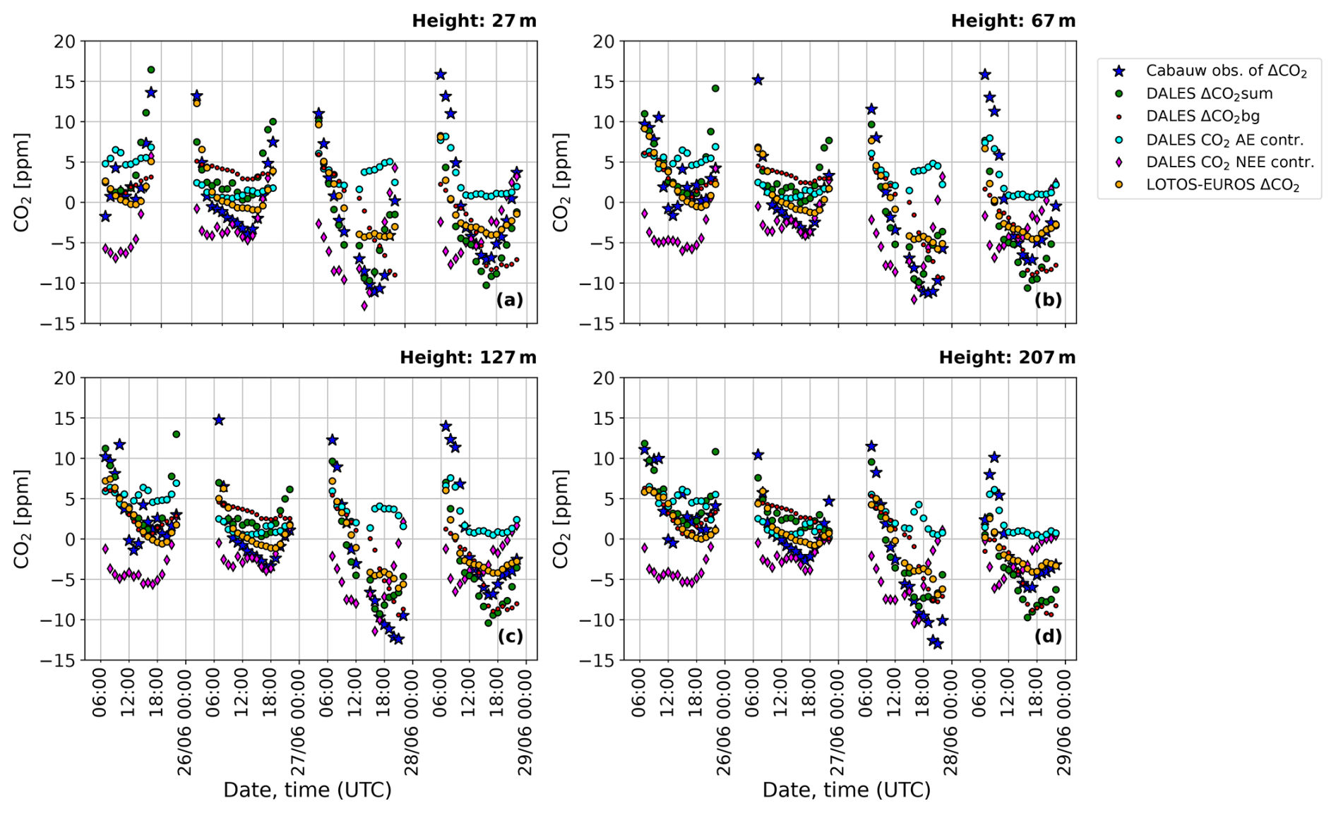
Figure 10Time series of observed and modeled CO2 mole fraction anomalies (ppm) at different levels of the Cabauw tower: (a) at 27 m, (b) at 67 m, (c) at 127 m, and (d) at 207 m. Blue stars: the anomalies of observed CO2; green circles: the modeled CO2 anomalies from DALES CO2sum; red circles: the modeled CO2 anomalies from DALES CO2bg; light blue: the contribution of all anthropogenic emissions (AEs) to the CO2 mole fraction from DALES; purple diamonds: the modeled NEE contribution to CO2 mole fractions from DALES; and orange circles: the modeled CO2 anomalies from LOTOS-EUROS. All values presented are calculated relative to the CO2 mean by subtracting the mean value (the average CO2 mole fraction over selected times(07:00–22:00 UTC) during the 25–28 June 2018 period). The values are averaged hourly, with the time corresponding to the end of the averaging period.
During this period, the AE contribution to CO2 mole fractions was generally low, with a mean of ∼2 ppm. Higher values of 5–7 ppm were observed during the early-morning hours due to nighttime near-surface accumulation effects. A reduced anthropogenic contribution is expected due to the rural location and wind direction, allowing for a comparison of biogenic and background variability in the models and observations for most of the selected period. A strong contribution from NEE in DALES CO2sum was observed, reaching values below −10 ppm.
DALES CO2sum tends to follow daytime variations more closely than LOTOS-EUROS does on 25, 27, and 28 June at lower levels (Fig. 10a, b), although it shows comparable values on 26 June, where the contribution from NEE is the lowest compared to other days ( ppm). The NEE contribution explains some of the daytime CO2 reduction due to photosynthesis, which is captured better in DALES than in LOTOS-EUROS. However, an underestimation of this decline remains, with observed CO2 values around 5 ppm lower than in DALES and 10 ppm lower than in LOTOS-EUROS. This underestimation could be explained in part by an offset in the background level, especially at times when the local CO2 loss due to photosynthesis is lower, such as in the late evening (see red dots in Fig. 10). Errors in the background concentration could result from the coarse resolution of the original CAMS dataset; from its 6 h update frequency, which may not capture finer temporal variations; and also from the lack of CO2 uptake by vegetation, which could cause the overestimated background (Bennouna et al., 2024). The offset in vertical mixing may also contribute, especially in the early-morning/late-evening hours.
At higher tower levels (Fig. 10c, d), the variability diminishes, which is consistent with the trapping of CO2 in a shallow surface layer during the early morning, although the biases relative to the observations persist. The AE contribution remains small, whereas the loss through CO2 uptake over the day persists strongly but with slightly lower values than at heights closer to the ground (by −2 ppm). The overestimation of the CO2 molar fraction during daytime, particularly in the late evening when the local contributions of NEE and AE are small, could be partially explained by the poorly resolved background and its deviation from observations (Bennouna et al., 2024). Furthermore, biases in the modeled wind speed and direction compared to observations could also contribute to discrepancies in CO2 variability (Zheng et al., 2019).
To further evaluate the accuracy of the simulations and quantify the degree of correspondence to measurements at the Cabauw tower, we performed a statistical regression analysis in the same way as for Westmaas and Slufter. The results of this analysis are shown in Fig. 11.
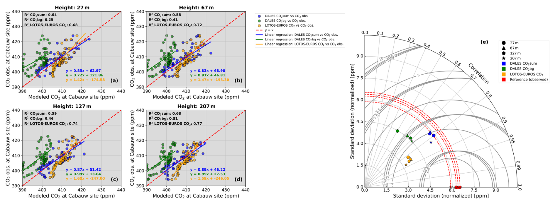
Figure 11(a–d) Density plots comparing model predictions (DALES CO2sum, CO2bg, and LOTOS-EUROS CO2) to observed CO2 mole fractions (ppm) at the Cabauw tower for the daytime (07:00–22:00 UTC) during the 25–28 June 2018 period at different heights: 27 m (a), 67 m (b), 127 m (c), and 207 m (d). The red dashed line represents the ideal relationship (y=x line). Linear regression lines are shown for CO2bg (green), CO2sum (blue), and LOTOS-EUROS CO2 (orange), along with the corresponding regression equations and R2 values. (e) Taylor diagram quantifying the model performance against observations. Circle: 27 m; triangle: 67 m; pentagon: 127 m; and star: 207 m. Blue: DALES CO2sum; green: DALES CO2bg; orange: LOTOS-EUROS CO2; and red: reference (observed CO2). Gray circular lines represent values of RMSD.
The predictions of DALES and LOTOS-EUROS show moderate performance (R2 values higher than 0.5) at capturing the CO2 variability in the measurements during daytime hours, with R2 values slightly higher for LOTOS-EUROS compared to DALES CO2sum at 27 m (R2: ∼ 0.64 vs. ∼ 0.68). However, at mid-level heights, this difference increases, with DALES showing a greater offset (R2: 0.58 vs. 0.72 at 67 m and 0.59 vs. 0.74 at 127 m). This may be in part due to background limitations, particularly on 26 and 28 June, when the contributions of AE and NEE to the CO2 mole fractions are minimal at the end of the day (see Fig. 10). At a 207 m height, the performance of both DALES CO2sum and LOTOS-EUROS slightly increases, exhibiting lower biases compared to the observations, with R2 values of 0.68 and 0.77, respectively.
The statistical metrics presented in the Taylor diagram (right panel of Fig. 11) illustrate the performance of different CO2 simulations (DALES CO2sum, DALES CO2bg, and LOTOS-EUROS) compared to observations at various altitudes. The diagram shows that LOTOS-EUROS better captures the observed variability in terms of correlation coefficients (which are closely related to R2), exceeding those of DALES CO2sum by approximately 5 %–10 %. However, some other metrics favor DALES CO2sum. Specifically, its normalized standard deviation closely matches observations at all heights, reproducing 85 %–90 % of the observed variability on average, whereas LOTOS-EUROS shows weaker agreement, capturing only about 50 % on average (see Fig. 10).
In terms of MBE, DALES CO2sum exhibits lower errors compared to LOTOS-EUROS at all heights (MBE: 27 m: −0.65 vs. 1.51; 67 m: 0.18 vs. 1.93; 127 m: 0.32 vs. 2.14; 207 m: 0.56 vs. 2.56). This indicates the slightly higher performance of DALES CO2sum at predicting mean CO2 levels for all heights during the daytime hours. Similarly, RMSE values are generally lower in DALES CO2sum or are comparable between the two at all altitudes (RMSE: 27 m: 3.93 vs. 4.16; 67 m: 4.25 vs. 4.25; 127 m: 4.24 vs. 4.47; 207 m: 3.42 vs. 4.28), indicating better general agreement with observed CO2 concentrations and a reduced tendency for large deviations.
Despite this, the RMSD values for DALES CO2sum are higher than those for LOTOS-EUROS at 67 m and 127 m, whereas at 27 m and 207 m, DALES CO2sum shows comparable or slightly better agreement (RMSD: 27 m: 3.87 vs. 3.87; 67 m: 4.25 vs. 3.78; 127 m: 4.23 vs. 3.92; 207 m: 3.37 vs. 3.43). This suggests that DALES CO2sum captures the observed variability slightly less accurately at mid-level heights, while at the lowest and highest measurement levels, it performs similarly to or marginally better than LOTOS-EUROS.
Nevertheless, while there are subtle differences between the two models, statistical metrics indicate that DALES CO2sum and LOTOS-EUROS exhibit good performance at the rural Cabauw site. During the period considered, both the local anthropogenic signal and the spatial variations in CO2 molar fractions remain relatively weak, and the precision of the simulations is largely determined by the background concentrations and the representation of the local biospheric contributions.
8.4 Contribution of modeled local CO2 components to regional CO2 enhancement
One of the objectives of this study is to examine the individual contributions of simulated individual flux components of atmospheric CO2 to the total CO2 that is observed at the measurement sites used in our study. To do this, we use the scalar CO2 tracers in DALES, from which the components of atmospheric CO2 can be easily determined (see Sect. 6.1). Figure 12 presents all these components for each measurement site separately.
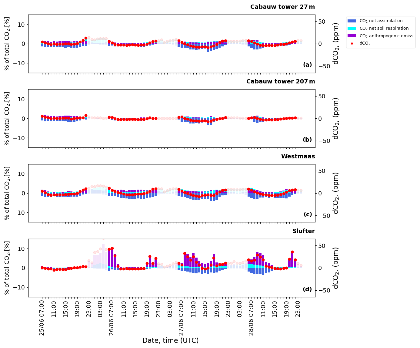
Figure 12The hourly averaged percentage contributions of various modeled local CO2 components to the overall atmospheric CO2 mole fraction (% of the full CO2 mole fraction) at three different measurement locations over the period from 25 to 28 June 2018. Cabauw tower at two heights, (a) 27 m and (b) 207 m, and near-surface CO2 (10 m) at (c) Westmaas and (b) Slufter. The colored bars represent the contributions from three components of atmospheric CO2: anthropogenic emissions (violet), CO2 soil respiration (cyan), and CO2 net assimilation (blue). The red dots represent dCO2, which is the deviation of total CO2 from the background (in ppm). Each bar in the plots starts from 0, and to avoid overlap, the position of positive bars is adjusted such that bars with lower values are displayed in front. The values are averaged hourly, with the time corresponding to the end of the averaging period.
At the Cabauw tower location, a clear diurnal pattern in atmospheric CO2 is observed at 27 m in height (Fig. 12a) and is diminished at 207 m in height (Fig. 12b). Here, CO2 net assimilation has the largest contribution during daytime, and soil respiration has the largest contribution during early morning/late evening (∼ 5 % in total), reflecting the contributions of biogenic activity. At a higher altitude of 207 m, the diurnal pattern in both CO2 biogenic components become smoother (∼2 %) due to the increased distance from the surface. The contribution from anthropogenic emissions is visible but in general remains tiny, especially at higher altitudes (within 5 ppm). As discussed above, the absence of large urban areas nearby and the northwest wind direction during this period (see Fig. 6) explain the low contribution of anthropogenic emissions to the CO2 variability during this period. Thus, in this area, the contribution of local agricultural emissions prevails, especially at the lowest tower level (see Fig. 4).
At the Westmaas site (Fig. 12c), we anticipated a higher local CO2 signal from anthropogenic emissions due to nearby urban areas. However, CO2 levels are only slightly above those measured at the lowest height at Cabauw (by 1 %–2 %). This smaller difference may be due to the lower elevation at Westmaas (10 m vs. 27 m at Cabauw) combined with plume dilution and vertical mixing, which could significantly reduce the anthropogenic CO2 reaching Westmaas during this period. The predicted variability in soil respiration contributes significantly to the total CO2 concentrations, particularly in the early morning/late evening (up to ∼ 5 %). Aside from this, as indicated in the CO2 NEE time series in Fig. 8, the negative contribution from the daytime photosynthesis CO2 sink offsets the positive contributions from both anthropogenic and soil respiration emissions, resulting in a net negative local contribution to the CO2 concentration during daytime throughout the period studied (by −3 %).
The Slufter site (Fig. 12d) displays a distinct pattern in which anthropogenic emissions play a dominant role in the local CO2 variability. When plumes from nearby facilities reach the measurement site, the anthropogenic contribution exceeds 10 % of the total CO2 mole fraction. The influence of net CO2 assimilation is also pronounced, although it is lower compared to the Westmaas site. The CO2 sink at Slufter is considerably weaker than at Westmaas, and it is insufficient to counterbalance the strong positive contributions of local anthropogenic activity, resulting in a strongly positive overall local contribution to the CO2 variability at this location throughout the simulation period.
These results demonstrate the ability of the new DALES framework to support the evaluation of local CO2 sources and their contributions to atmospheric CO2 concentrations. The weak signal of anthropogenic emissions at the Cabauw tower, particularly at higher tower levels, contrasts sharply with the more urban or industrially influenced sites such as Slufter, where anthropogenic sources dominate. Aside from this, we show that biogenic CO2 fluxes contribute significantly to diurnal variability. Even in Westmaas, a short distance from the port and center of Rotterdam, the biogenic component contributes significantly to the simulated diurnal CO2 variability (see also Fig. 8). This highlights the importance of an accurate representation of biogenic sources in the high-resolution modeling of urban CO2 variability.
Despite significant progress integrating CO2 emissions into the LES model presented in this study, it is essential to address existing limitations and challenges to enable further improvements and more accurate future implementations.
In our work, we mentioned the limitations of LESs when reproducing the observed variability, particularly under stable boundary layer conditions as well as in the coastal environment, as revealed in observations at Slufter. Although LES models still face challenges related to the accurate simulation of nocturnal stable ABL conditions, proposed solutions have been developed to better resolve turbulence in stable boundary layers at coarser horizontal resolutions (>10 m) (de Roode et al., 2017; Dai et al., 2021). However, the verification of these methods is still ongoing, and the corresponding routines have yet to be implemented in the community version of DALES. The coastal environment is also an area for further improvement in LESs, especially the integration of a more accurate marine atmosphere in high-resolution models, which is planned to be done in the next few years by the team from Ruisdael Observatory. Achieving this will require an even finer spatial resolution to resolve the complex processes in the coastal environment. However, while DALES has the potential to operate at horizontal resolutions as fine as 1 m, the current 100 m resolution used in our setup is a compromise, balancing computational feasibility and domain size. These constraints are partly introduced by the meteorological data resolution from the HARMONIE-AROME model, which currently operates at a ∼ 2.5 km resolution (N25 grid). However, from 2024 on, HARMONIE-AROME has switched to the N20 grid, featuring a finer horizontal resolution (∼ 1.3 km), which could enhance LES accuracy, particularly in regions with strong local CO2 sources. The 6 h temporal resolution of the 0.125°×0.125° CAMS EGG4 reanalysis data used in our study limits its ability to reproduce the observed diurnal CO2 variability. However, recent CAMS datasets, offering 3 h data and a higher horizontal resolution (0.1°×0.1°), may improve the CO2 background representation in future simulations (https://ads.atmosphere.copernicus.eu/datasets/cams-global-greenhouse-gas-forecasts?tab=overview, last access: 27 November 2024). Despite the bias correction applied in CAMS EGG4 (Bennouna et al., 2024), it does not employ flux inversion techniques to optimize CO2 surface fluxes, unlike the optimized CAMS products with a lower spatiotemporal resolution (e.g. https://ads.atmosphere.copernicus.eu/datasets/cams-global-greenhouse-gas-inversion?tab=overview, last access: 11 March 2025). However, the spatiotemporal resolution of optimized CAMS is still a limitation. An alternative approach is to use, for example, the LOTOS-EUROS output, with its finer horizontal and temporal resolution (up to 1 km and hourly output), coupled with DALES, which could enhance the representation of background variability in chemical compounds. To increase the accuracy of LES-simulated CO2 variability, there is a plan to switch from nudged to open boundary conditions. This has been shown to enhance the accuracy and applicability of the LES framework across diverse atmospheric conditions (Liqui Lung et al., 2024).
Aside from this, attention should be paid to the further improvement of anthropogenic emissions input. The national emission inventory for the Netherlands is constantly updated, and data are expected to be more accurate in the future (Van der Net et al., 2024). In the meantime, ensemble experiments incorporating perturbations in anthropogenic emissions will be performed to address this uncertainty in the modeling. The need for high-resolution activity and proxy data to advance the downscaling workflow and improve the emission input preparation for LES is also an important area for further work. Additional refinement could be achieved through the use of high-resolution monitoring data, such as ship traffic and waterway data, as well as detailed agricultural land use information across the Netherlands (van der Woude et al., 2023, https://www.clo.nl/en/indicators/en006111-land-use-in-the-netherlands-2015, last access: 27 November 2024).
Moreover, the vertical allocation of emissions and plume rise should be further improved. In the setup used in this study (with a 100 m horizontal resolution), plume rise is a subgrid process; therefore, using a parameterization is an appropriate approach. An alternative to the approach adopted here could be to address plume rise in LESs by prescribing a heat source in the potential temperature equation at the location of the chimney top. This method enables LESs to compute the heating tendency, which in turn modifies the vertical velocity through its effect on buoyancy. A key challenge is to accurately estimate the heat production of the stack, which represents the energy added by the emission of heated air per unit of time. This would also help represent the interactions of the emission plume and the ambient meteorological conditions. Note that this works if the model grid is very fine (< 50 m) and if the plume is narrow compared to the grid. Furthermore, our plume rise algorithm does not yet consider the influence of the emitting plume on local meteorology, such as thermal and radiative effects on atmospheric stability (Lohmann and Feichter, 2005).
In DALES, the vertical profiles are not source specific but are rather a simplified even distribution of the emissions between the calculated bottom and top of the plume for SNAP categories, which include the vertical component. As pointed out by Brunner et al. (2019), there are benefits to applying accurate category-specific emission initial vertical distributions.
In addition, LESs can optimize emissions for specific SNAP categories by integrating top-down atmospheric observations with bottom-up inventories. This approach refines the spatial and temporal distribution of emissions, providing a high-resolution benchmark for validating and adjusting reported estimates. However, the use of LESs in atmospheric transport inversions poses several challenges. This includes the limited spatial and temporal extent of LES domains that restrict inversions to local or short-term events. This requires careful nesting within larger-scale models to capture background conditions accurately (see, e.g., Barlow et al., 2011; Lauvaux et al., 2016). Aside from this, high computational costs also constrain the ensemble size and averaging periods required for robust inversions. Although analytical inversions may be feasible for a limited number of tracers or emission parameters, the high dimensionality and inherent nonlinear dynamics of LES simulations generally require ensemble-based methods (e.g., Brunner et al., 2019). Despite these challenges, LES-based inversions offer a valuable framework for process-level understanding and can serve as a benchmark for evaluating bottom-up inventories under well-constrained conditions.
As this study shows, the results are sensitive to the representation of biogenic CO2 fluxes, even at short distances from urban centers. Hence, future efforts should also improve the representation of these fluxes at the resolution of the model, moving beyond our highly simplified split between grasslands and forests. In the case of intensive agriculture in the Netherlands, this is complicated by the significant role of management. The measurement from the Loobos observation station made by Ruisdael Observatory can be helpful in this context, as this station is in the forested area at distance from important anthropogenic emissions but with a region of intensive agriculture to the west. Thus, validating the biogenic fluxes from LESs at the Loobos location would be beneficial. In addition, the incorporation of forested land may be upgraded to consider the vertical height of the forest, which also influences the simulated atmospheric dynamics. It may require a large upgrade to the model code, including the possible implementation of the flexibility of tree representation if the model resolution changes. However, even much less sophisticated solutions could bring about important improvements. The same holds for the representation of urban landscapes. Currently, three-dimensional city maps for the Netherlands are under construction at TU Delft (https://3d.bk.tudelft.nl/projects/, last access: 27 November 2024).
We present a new atmospheric modeling platform to simulate the spatiotemporal CO2 concentration at a hectometer resolution. The main novelty is the explicit calculation of the turbulent mixing and transport of CO2 in the Dutch environment by means of the Dutch atmospheric LES. In this work, we present and discuss a workflow for downscaling the kilometer-scale national emission inventory, consisting of point and area diffuse sources, to 100 m scale DALES input.
We extended DALES with methodology to account for the vertical distribution of emissions from elevated point sources, including the modeling of plume rise. This is done using an online algorithm that considers the interaction between the plume properties and ambient atmospheric conditions. To represent biogenic CO2 fluxes from respiration and photosynthesis, DALES has been extended with a simplified land surface model that differentiates between grasslands and forests. The performance of DALES has been evaluated using the LOTOS-EUROS model and the available in situ observations for daytime (07:00–22:00 UTC) during a 4 d test period in June 2018. A rigorous statistical analysis quantifies the benefits of the high-resolution-modeling approach, particularly near urban and industrial areas. This is evident in the standard deviations, which are closer to the observed values across all measurement sites, and the generally lower RMSD. For instance, DALES CO2sum in Slufter has an SD of 15.27 ppm, closely matching the observed SD of 12.23 ppm, compared to 5.93 ppm in LOTOS-EUROS. A similar trend is observed at the Cabauw tower, where DALES explains more than 85 % of the variability in terms of standard deviation at all heights compared to less than 50 % in LOTOS-EUROS. Additionally, DALES CO2sum in Westmaas shows better performance, with R2 and correlation values of 0.69 and 0.83, along with a lower RMSD of 3.76 ppm compared to the LOTOS-EUROS values of 0.48, 0.69, and 4.93 ppm, respectively (see Table A2 for more details). Aside from this, we identified limitations in the current framework, such as larger deviations from observations at the Cabauw rural location and challenges simulating coastal environments, which will require further improvement in future developments.
A multi-tracer approach is used to keep track of the contribution of anthropogenic and biogenic fluxes to the simulated CO2 concentrations. This analysis enhanced our understanding of the relative importance of their contributions, explaining the CO2 variability in the measurements that have been used. The significant variations in CO2 concentration observed at Slufter on the Maasvlakte at the western tip of the Rotterdam harbor are largely explained by anthropogenic activity (up to 10 % of total CO2 for the period considered). The importance of ecosystem fluxes of CO2 has been demonstrated, even in close proximity to urban and industrial CO2 emissions. These fluxes largely contribute to the CO2 concentration variability during daytime, when they may even cancel out local anthropogenic concentration enhancements (as seen in Cabauw and Westmaas, where the daytime contribution of local CO2 is negative, reaching −3 %), emphasizing the importance of an accurate representation of biogenic processes in the modeling of urban CO2.
The DALES framework has significant potential to advance atmospheric CO2 concentration modeling and support the independent evaluation of national emission inventories at the urban scale. This framework is expected to facilitate the quantification of local emission hotspots in combination with inversion techniques, while also reinforcing air quality monitoring efforts. Furthermore, by delivering detailed information on subgrid processes, such as turbulence, boundary layer dynamics, and localized emission dispersion, DALES can enhance parameterizations in larger-scale models through nesting, contributing to more accurate regional climate predictions (Sun, 2016). Ultimately, these advances will support more informed decision-making (e.g., using the LES output to refine long-term forecasts with mesoscale models or incorporating AI) and the formulation of effective policies aimed at mitigating climate change and its associated impacts in the Netherlands and beyond.
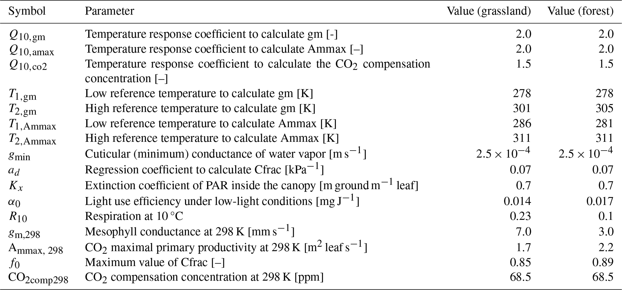
Table A2Statistical metrics to evaluate the robustness of model performance against measurements at the Cabauw, Westmaas, and Slufter locations. n/a – not applicable
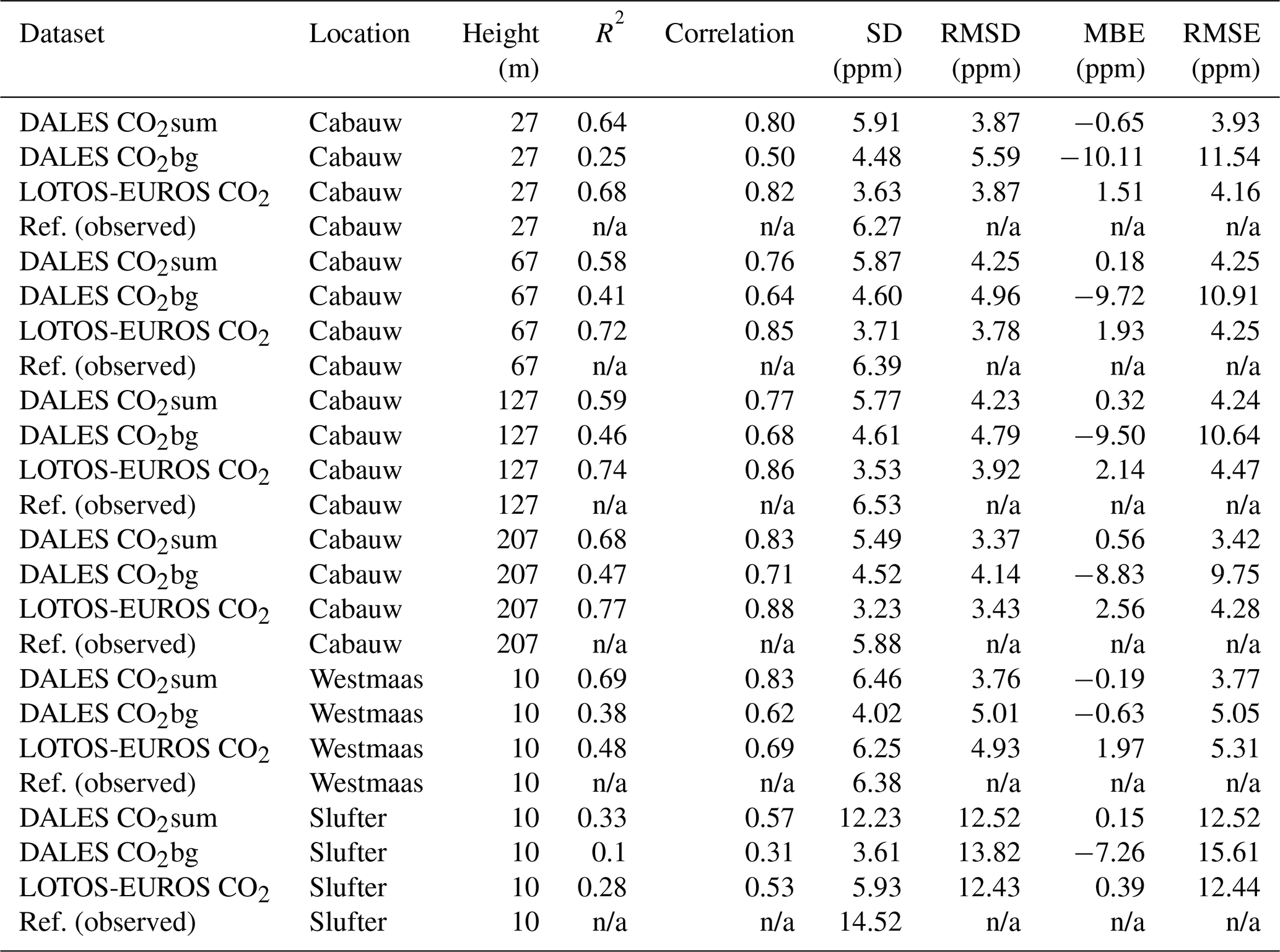
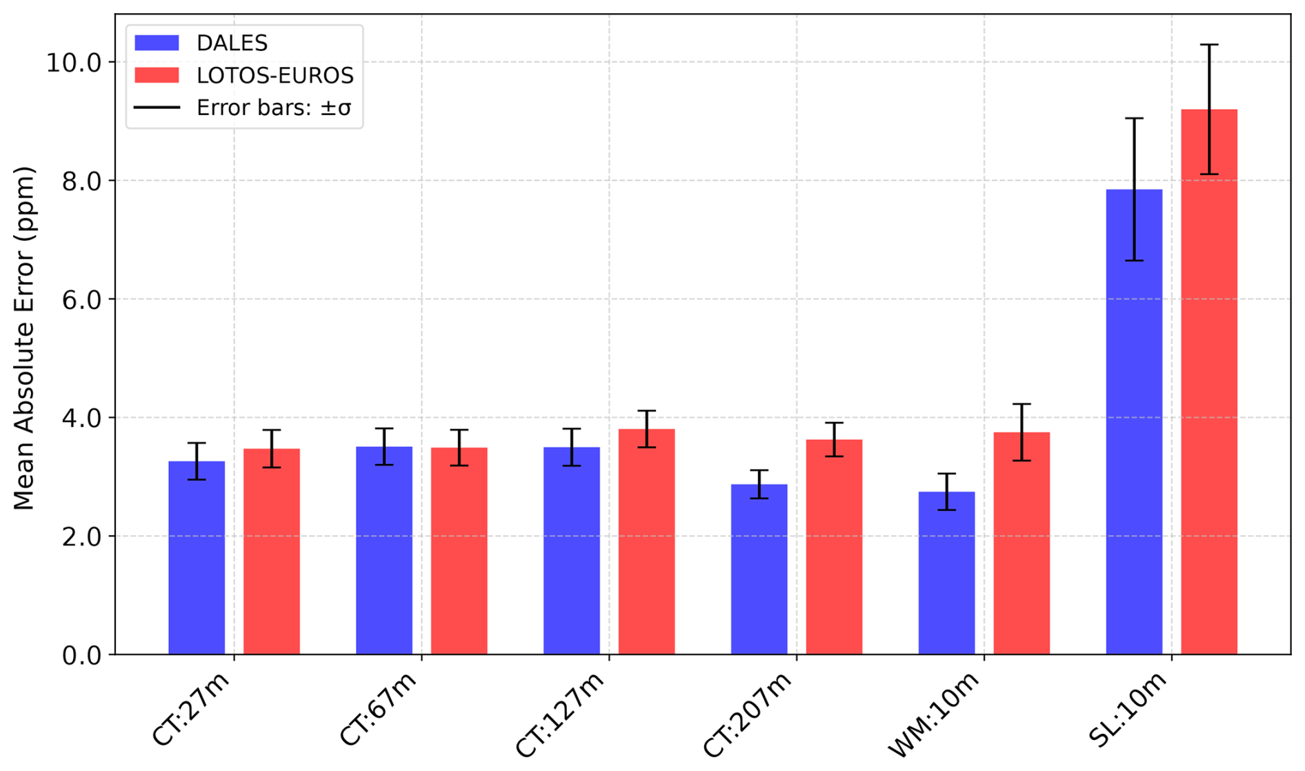
Figure B1Bootstrap analysis (1000 iterations) of the mean absolute error (MAE) between model predictions (DALES CO2sum and LOTOS-EUROS CO2) and CO2 observations at multiple heights and locations. The bars represent the mean MAE, with error bars indicating ±σ based on bootstrap sampling. Locations and specific heights are labeled below the bars: CT:27m – Cabauw tower at 27 m; CT:67m – Cabauw tower at 67 m; CT:127m – Cabauw tower at 127 m; CT:207m – Cabauw tower at 207 m; WM:10m – Westmaas at 10 m; and SL:10m – Slufter at 10 m.
The emission inventories used in this study were obtained from the Emission Registration (ER) portal, processed by the National Institute of Public Health and the Environment (RIVM), and are accessible at https://data.emissieregistratie.nl/export, last access: 27 November 2024. Dutch Atmospheric Large-Eddy Simulation (DALES) 4.4, with the emission module that was developed in this study, is open-source code available under GNU GPL version 3. This specific version of the DALES model is available on the Zenodo repository (https://doi.org/10.5281/zenodo.14216703, Karagodin-Doyennel, 2024a). HARMONIE-AROMA model data on a rectilinear grid, specifically the “Winds of the North Sea in 2050” (WINS50) dataset covering the Netherlands with a 1 h temporal resolution, are available at https://dataplatform.knmi.nl/dataset/wins50-wfp-nl-ts-singlepoint-3 Royal Netherlands Meteorological Institute, 2025. CAMS (Copernicus Atmosphere Monitoring Service) data can be freely accessed at https://ads.atmosphere.copernicus.eu/ (last access: 27 November 2024, Agustí-Panareda et al., 2023). The complete “offline” emission downscaling workflow program, developed and utilized in this study, is open-source and freely accessible code available at https://doi.org/10.5281/zenodo.14216478 (Karagodin-Doyennel, 2024b). The CBS Vierkant 100 × 100 m and ESRI shapefile datasets, which were used in the downscaling procedure, are available on the CBS website: https://www.cbs.nl/nl-nl/dossier/nederland-regionaal/geografische-data/kaart-van-100-meter-bij-100-meter-met-statistieken (Centraal Bureau voor de Statistiek, 2025). The annual NOx emission traffic shapefile can be accessed from the Zenodo repository: https://doi.org/10.5281/zenodo.14961517 (Karagodin-Doyennel, 2025). The atmospheric CO2 data from the Cabauw measurement site used for validation in this study are publicly available via the ICOS Carbon Portal. The data include multiple height levels spanning different time periods. The datasets can be accessed as follows. Cabauw (27.0 m): https://hdl.handle.net/11676/2VWHcamWul6f99NFnynnZD7L (Frumau et al., 2024a). Cabauw (67.0 m): https://hdl.handle.net/11676/-T_0NVoAGVxkifBvqbErBCbY (Frumau et al., 2024b). Cabauw (127.0 m): https://hdl.handle.net/11676/0k14wqlTJO_K2HcrDaTMHlhp (Frumau et al., 2024c). Cabauw (207.0 m): https://hdl.handle.net/11676/6ND_CiR0NY4HBBddqsdh_raU (Frumau et al., 2024d).
AKD developed the emission downscaling workflow and DALES extensions, performed all simulations, handled the visualization, and wrote the original draft with formal analysis. JVGdA and BJHvS assisted with the integration of forest components into the A-gs scheme and contributed to the analysis of the results. HDvdG was responsible for the TNO observational data description and assisted with the analysis. FJ supported the software implementation and the initial processing of data for assimilation and assisted in the model development. SH conceptualized the research work, developed the methodology, and contributed to the writing and analysis of the results. All the authors participated in editing the paper and discussing the results.
The contact author has declared that none of the authors has any competing interests.
Publisher’s note: Copernicus Publications remains neutral with regard to jurisdictional claims made in the text, published maps, institutional affiliations, or any other geographical representation in this paper. While Copernicus Publications makes every effort to include appropriate place names, the final responsibility lies with the authors.
We are grateful to the Dutch Research Council (NWO) for financial support of this research as part of the Ruisdael Observatory scientific research infrastructure (grant no. 184.034.015). We also extend our thanks to RIVM, especially to Margreet van Zanten, Romuald te Molder, and Jolien van Huystee, for providing comprehensive emissions datasets, plume thermal properties, assistance in the description of the datasets and properties, and fruitful discussion. We thank Arjo Segers from TNO for providing LOTOS-EUROS simulation data and for discussion on the setup. Additionally, we thank DAT.MOBILITY, particularly Eric Pijnappels, for granting access to the NOx traffic emission data used in this research. We are also grateful to ICOS for the opportunity to use CO2 measurements from the Cabauw tower. Finally, we acknowledge SURFSARA for providing the computational resources to conduct the simulations for this study and NWO for supporting the project budget through the National Roadmap for Large-Scale Research Facilities (https://www.nwo.nl/en/researchprogrammes/national-roadmap-for-large-scale-research-facilities, last access: 27 November 2024).
This research has been supported by the Nederlandse Organisatie voor Wetenschappelijk Onderzoek (grant no. 184.034.015).
This paper was edited by Bo Zheng and reviewed by two anonymous referees.
Agustí-Panareda, A., Barré, J., Massart, S., Inness, A., Aben, I., Ades, M., Baier, B. C., Balsamo, G., Borsdorff, T., Bousserez, N., Boussetta, S., Buchwitz, M., Cantarello, L., Crevoisier, C., Engelen, R., Eskes, H., Flemming, J., Garrigues, S., Hasekamp, O., Huijnen, V., Jones, L., Kipling, Z., Langerock, B., McNorton, J., Meilhac, N., Noël, S., Parrington, M., Peuch, V.-H., Ramonet, M., Razinger, M., Reuter, M., Ribas, R., Suttie, M., Sweeney, C., Tarniewicz, J., and Wu, L.: Technical note: The CAMS greenhouse gas reanalysis from 2003 to 2020, Atmos. Chem. Phys., 23, 3829–3859, https://doi.org/10.5194/acp-23-3829-2023, 2023. a
Akingunola, A., Makar, P. A., Zhang, J., Darlington, A., Li, S.-M., Gordon, M., Moran, M. D., and Zheng, Q.: A chemical transport model study of plume-rise and particle size distribution for the Athabasca oil sands, Atmos. Chem. Phys., 18, 8667–8688, https://doi.org/10.5194/acp-18-8667-2018, 2018. a, b, c, d, e
Arakawa, A., Jung, J.-H., and Wu, C.-M.: Toward unification of the multiscale modeling of the atmosphere, Atmos. Chem. Phys., 11, 3731–3742, https://doi.org/10.5194/acp-11-3731-2011, 2011. a
Arakawa, A., Jung, J.-H., and Wu, C.-M.: Multiscale modeling of the moist-convective atmosphere, Meteorol. Monogr., 56, 16.1–16.17, https://doi.org/10.1175/AMSMONOGRAPHS-D-15-0014.1, 2016. a
Balsamo, G., Beljaars, A. C. M., Scipal, K., Viterbo, P., Van den Hurk, B., Hirschi, M., and Betts, A. K.: A revised hydrology for the ECMWF model: Verification from field site to terrestrial water storage and impact in the Integrated Forecast System, J. Hydrometeorol.y, 10, 623–643, 2009. a
Barlow, J. F., Dunbar, T. M., Nemitz, E., Wood, C. R., Gallagher, M. W., Davies, F., O'Connor, E., Harrison, R. M., Robins, A. G., and Grimmond, S.: Developing a neighbourhood-scale flux measurement capability for the UK: The CityFlux project, Philos. T. Roy. Soc. A, 369, 3477–3490, https://doi.org/10.1098/rsta.2011.0053, 2011. a
Bengtsson, L., Körnich, H., Andrae, U., Aspelien, T., Batrak, Y., Calvo, J., de Rooy, W., Gleeson, E., Hansen-Sass, B., Homleid, M., Hortal, M., Ivarsson, K.-I., Lenderink, G., Niemelä, S., Nielsen, K. P., Onvlee, J., Rontu, L., Samuelsson, P., Muñoz, D. S., Subias, A., Tijm, S., Toll, V., Yang, X., and Ødegaard Køltzow, M.: The HARMONIE–AROME model configuration in the ALADIN–HIRLAM NWP system, Mon. Weather Rev., 145, 1919–1935, https://doi.org/10.1175/MWR-D-16-0417.1, 2017. a
Bennouna, Y., Eskes, H. J., Kouyate, M., Langerock, B., Pison, I., Ramonet, M., Tsikerdekis, A., and Warneke, T.: Validation report for the EGG4 version 2 global reanalysis: 2003–2023, Technical Report CAMS2_82_2023SC2_D82.4.2.2-2024, Copernicus Atmosphere Monitoring Service (CAMS), https://doi.org/10.24380/jcyt-ppgt, 2024. a, b, c, d
Briggs, G. A.: Plume rise and buoyancy effects, atmospheric sciences and power production, in: DOE/TIC-27601 (DE84005177), edited by: Randerson, D., Technical Information Center, U.S. Dept. of Energy, Oak Ridge, USA, 327–366, 1984. a, b, c
Brioude, J., Petron, G., Frost, G. J., Ahmadov, R., Angevine, W. M., Hsie, E.-Y., Kim, S.-W., Lee, S.-H., McKeen, S. A., Trainer, M., Fehsenfeld, F. C., Holloway, J. S., Peischl, J., Ryerson, T. B., and Gurney, K. R.: A new inversion method to calculate emission inventories without a prior at mesoscale: Application to the anthropogenic CO2 emission from Houston, Texas, J. Geophys. Res.-Atmos., 117, D05312, https://doi.org/10.1029/2011JD016918, 2012. a
Brunner, D., Kuhlmann, G., Marshall, J., Clément, V., Fuhrer, O., Broquet, G., Löscher, A., and Meijer, Y.: Accounting for the vertical distribution of emissions in atmospheric CO2 simulations, Atmos. Chem. Phys., 19, 4541–4559, https://doi.org/10.5194/acp-19-4541-2019, 2019. a, b, c, d, e, f, g
Brunner, D., Kuhlmann, G., Henne, S., Koene, E., Kern, B., Wolff, S., Voigt, C., Jöckel, P., Kiemle, C., Roiger, A., Fiehn, A., Krautwurst, S., Gerilowski, K., Bovensmann, H., Borchardt, J., Galkowski, M., Gerbig, C., Marshall, J., Klonecki, A., Prunet, P., Hanfland, R., Pattantyús-Ábrahám, M., Wyszogrodzki, A., and Fix, A.: Evaluation of simulated CO2 power plant plumes from six high-resolution atmospheric transport models, Atmos. Chem. Phys., 23, 2699–2728, https://doi.org/10.5194/acp-23-2699-2023, 2023. a, b, c
Centraal Bureau voor de Statistiek (CBS): CBS Vierkant 100 × 100 m and ESRI Shapefile Datasets, https://www.cbs.nl/nl-nl/dossier/nederland-regionaal/geografische-data/kaart-van-100-meter-bij-100-meter-met-statistieken, last access: 20 July 2025. a
Crippa, M., Solazzo, E., Huang, G., Guizzardi, D., Koffi, B., Muntean, M., Schaaf, E., Friedrich, R., and Janssens-Maenhout, G.: High resolution temporal profiles in the Emissions Database for Global Atmospheric Research, Sci. Data, 7, 121, https://doi.org/10.1038/s41597-020-0462-2, 2020. a
Dai, Y., Basu, S., Maronga, B., and de Roode, S. R.: Addressing the grid-size sensitivity issue in large-eddy simulations of stable boundary layers, Bound.-Lay. Meteorol., 178, 63–89, 2021. a, b
de Bruine, M., Krol, M., Vilà-Guerau de Arellano, J., and Röckmann, T.: Explicit aerosol–cloud interactions in the Dutch Atmospheric Large-Eddy Simulation model DALES4.1-M7, Geosci. Model Dev., 12, 5177–5196, https://doi.org/10.5194/gmd-12-5177-2019, 2019. a
de Bruine, M., Jansson, F., van Stratum, B., Rijsdijk, P., and Houweling, S.: Simulating the emission and transport of gases on 100-meter resolution in a 100-kilometer domain, in: EGU General Assembly 2021, online, https://doi.org/10.5194/egusphere-egu21-13055, 2021. a
de Roode, S. R., Jonker, H. J., van de Wiel, B. J., Vertregt, V., and Perrin, V.: A diagnosis of excessive mixing in Smagorinsky subfilter-scale turbulent kinetic energy models, J. Atmos. Sci., 74, 1495–1511, 2017. a
Deardorff, J. W.: Numerical investigation of neutral and unstable planetary boundary layers, J. Atmos. Sci., 29, 91–115, 1972. a
Denier van der Gon, H. A. C., Dellaert, S. N. C., Super, I., Visschedijk, A. J. H., Janssens-Maenhout, G., Guizzardi, D., Pinto, A., Petrescu, A.-M. R., Crippa, M., López-Bon, R., Bousserez, N., Broquet, G., Engelen, R. J., Haussaire, J.-M., Petrescu, R., Chevallier, F., Peylin, P., and Segers, A. J.: Deliverable Report D2.2: Prior Emissions Data 2021 Documentation Report [tech. rep.], CoCO2 project, https://coco2-project.eu/sites/default/files/2023-04/CoCO2-D2.2-V1-2.pdf (last access: 20 July 2025), 2021. a
Dosio, A., Vilà-Guerau de Arellano, J., Holtslag, A. A. M., and Builtjes, P. J. H.: Dispersion of a Passive Tracer in Buoyancy- and Shear-Driven Boundary Layers, J. Appl. Meteorol. Clim., 42, 1116–1130, https://doi.org/10.1175/1520-0450(2003)042<1116:DOAPTI>2.0.CO;2, 2003. a
Doyennel, A.: Annual NOx emission traffic shape file, Zenodo [data set], https://doi.org/10.5281/zenodo.14961517, 2025. a
EEA: Emission Inventory Guidebook, https://www.eea.europa.eu/publications/EMEPCORINAIR/partb.pdf (last access: 13 March 2025), 1999. a
Fischereit, J., Vedel, H., Larsén, X. G., Theeuwes, N. E., Giebel, G., and Kaas, E.: Modelling wind farm effects in HARMONIE–AROME (cycle 43.2.2) – Part 1: Implementation and evaluation, Geosci. Model Dev., 17, 2855–2875, https://doi.org/10.5194/gmd-17-2855-2024, 2024. a
Frumau, A., Hensen, A., and Vermeulen, A.: Atmospheric CO2 product, Cabauw (27.0 m), 2000-01-01–2024-03-31, European ObsPack, https://hdl.handle.net/11676/2VWHcamWul6f99NFnynnZD7L (last access: 20 July 2025) 2024a. a, b
Frumau, A., Hensen, A., and Vermeulen, A.: Atmospheric CO2 product, Cabauw (67.0 m), 2000-01-01–2024-03-31, European ObsPack, https://hdl.handle.net/11676/-T_0NVoAGVxkifBvqbErBCbY (last access: 20 July 2025) 2024b. a, b
Frumau, A., Hensen, A., and Vermeulen, A.: Atmospheric CO2 product, Cabauw (127.0 m), 2000-01-01–2024-03-31, European ObsPack, https://hdl.handle.net/11676/0k14wqlTJO_K2HcrDaTMHlhp (last access: 20 July 2025) 2024c. a, b
Frumau, A., Hensen, A., and Vermeulen, A.: Atmospheric CO2 product, Cabauw (207.0 m), 1992-10-23–2024-03-31, European ObsPack, https://hdl.handle.net/11676/6ND_CiR0NY4HBBddqsdh_raU (last access: 20 July 2025), 2024d. a, b
Gordon, M., Makar, P. A., Staebler, R. M., Zhang, J., Akingunola, A., Gong, W., and Li, S.-M.: A comparison of plume rise algorithms to stack plume measurements in the Athabasca oil sands, Atmos. Chem. Phys., 18, 14695–14714, https://doi.org/10.5194/acp-18-14695-2018, 2018. a, b
Guevara, M., Tena, C., Porquet, M., Jorba, O., and Pérez García-Pando, C.: HERMESv3, a stand-alone multi-scale atmospheric emission modelling framework – Part 1: global and regional module, Geosci. Model Dev., 12, 1885–1907, https://doi.org/10.5194/gmd-12-1885-2019, 2019. a
Guevara, M., Enciso, S., Tena, C., Jorba, O., Dellaert, S., Denier van der Gon, H., and Pérez García-Pando, C.: A global catalogue of CO2 emissions and co-emitted species from power plants, including high-resolution vertical and temporal profiles, Earth Syst. Sci. Data, 16, 337–373, https://doi.org/10.5194/essd-16-337-2024, 2024. a
Hazan, L., Tarniewicz, J., Ramonet, M., Laurent, O., and Abbaris, A.: Automatic processing of atmospheric CO2 and CH4 mole fractions at the ICOS Atmosphere Thematic Centre, Atmos. Meas. Tech., 9, 4719–4736, https://doi.org/10.5194/amt-9-4719-2016, 2016. a
Heus, T., van Heerwaarden, C. C., Jonker, H. J. J., Pier Siebesma, A., Axelsen, S., van den Dries, K., Geoffroy, O., Moene, A. F., Pino, D., de Roode, S. R., and Vilà-Guerau de Arellano, J.: Formulation of the Dutch Atmospheric Large-Eddy Simulation (DALES) and overview of its applications, Geosci. Model Dev., 3, 415–444, https://doi.org/10.5194/gmd-3-415-2010, 2010. a, b, c
Huo, D., Huang, X., Dou, X., Ciais, P., Li, Y., Deng, Z., Wang, Y., Cui, D., Benkhelifa, F., Sun, T., Zhu, B., Roest, G., Gurney, K. R., Ke, P., Guo, R., Lu, C., Lin, X., Lovell, A., Appleby, K., DeCola, P. L., Davis, S. J., and Liu, Z.: Carbon Monitor Cities near-real-time daily estimates of CO2 emissions from 1500 cities worldwide, Sci. Data, 9, 533, https://doi.org/10.1038/s41597-022-01657-z, 2022. a
IPCC: Summary for Policymakers, Cambridge University Press, Cambridge, United Kingdom and New York, NY, USA, https://doi.org/10.1017/9781009157896, 2021. a
IPCC: Summary for Policymakers, IPCC, Geneva, Switzerland, https://doi.org/10.59327/IPCC/AR6-9789291691647.001, 2023. a, b
Jacobs, A., Heusinkveld, B., and Holtslag, A.: Seasonal and interannual variability of carbon dioxide and water balances of a grassland, Climatic Change, 82, 163–177, https://doi.org/10.1007/s10584-006-9182-7, 2007. a, b
Jacobs, C. M. J. and de Bruin, H. A. R.: Predicting of regional transpiration at elevated atmospheric CO2: influence of the PBL vegetation interaction, J. Appl. Meteorol., 36, 1663–1675, https://doi.org/10.1175/1520-0450(1997)036<1663:PRTAEA>2.0.CO;2, 1997. a, b
Jähn, M., Kuhlmann, G., Mu, Q., Haussaire, J.-M., Ochsner, D., Osterried, K., Clément, V., and Brunner, D.: An online emission module for atmospheric chemistry transport models: implementation in COSMO-GHG v5.6a and COSMO-ART v5.1-3.1, Geosci. Model Dev., 13, 2379–2392, https://doi.org/10.5194/gmd-13-2379-2020, 2020. a
Jia, G., Huang, Z., Tang, X., Ou, J., Lu, M., Xu, Y., Zhong, Z., Sha, Q., Wu, H., Zheng, C., Deng, T., Chen, D., He, M., and Zheng, J.: A meteorologically adjusted ensemble Kalman filter approach for inversing daily emissions: A case study in the Pearl River Delta, China, J. Environ. Sci., 114, 233–248, https://doi.org/10.1016/j.jes.2021.08.048, 2021. a
Karagodin-Doyennel, A.: DALES 4.4 emission, (1.0), Zenodo [code], https://doi.org/10.5281/zenodo.14216703, 2024a. a, b
Karagodin-Doyennel, A.: Emission inventory workflow, (1.0), Zenodo [code], https://doi.org/10.5281/zenodo.14216478, 2024b. a, b
Karagodin-Doyennel, A.: Annual NOx emission traffic shape file (1.0), Zenodo [data set], https://doi.org/10.5281/zenodo.14961517, 2025. a
Kuenen, J., Dellaert, S., Visschedijk, A., Jalkanen, J.-P., Super, I., and Denier van der Gon, H.: CAMS-REG-v4: a state-of-the-art high-resolution European emission inventory for air quality modelling, Earth Syst. Sci. Data, 14, 491–515, https://doi.org/10.5194/essd-14-491-2022, 2022. a
Lauvaux, T., Miles, N. L., Richardson, S. J., Cambaliza, M. O., Davis, K. J., Deng, A., Gaudet, B., Gurney, K. R., Huang, J., Oda, T., Prasad, K., Sarmiento, D. P., Shepson, P. B., Turnbull, J. C., and Wu, K.: High-resolution atmospheric inversion of urban CO2 emissions during the dormant season of the Indianapolis Flux Experiment (INFLUX), Journal of Geophysical Research: Atmospheres, 121, 5213–5236, https://doi.org/10.1002/2015JD024473, 2016. a
Liqui Lung, F., Jakob, C., Siebesma, A. P., and Jansson, F.: Open boundary conditions for atmospheric large-eddy simulations and their implementation in DALES4.4, Geosci. Model Dev., 17, 4053–4076, https://doi.org/10.5194/gmd-17-4053-2024, 2024. a
Liu, Y., Gruber, N., and Brunner, D.: Spatiotemporal patterns of the fossil-fuel CO2 signal in central Europe: results from a high-resolution atmospheric transport model, Atmos. Chem. Phys., 17, 14145–14169, https://doi.org/10.5194/acp-17-14145-2017, 2017. a, b
Lohmann, U. and Feichter, J.: Global indirect aerosol effects: a review, Atmos. Chem. Phys., 5, 715–737, https://doi.org/10.5194/acp-5-715-2005, 2005. a
Manders, A. M. M., Builtjes, P. J. H., Curier, L., Denier van der Gon, H. A. C., Hendriks, C., Jonkers, S., Kranenburg, R., Kuenen, J. J. P., Segers, A. J., Timmermans, R. M. A., Visschedijk, A. J. H., Wichink Kruit, R. J., van Pul, W. A. J., Sauter, F. J., van der Swaluw, E., Swart, D. P. J., Douros, J., Eskes, H., van Meijgaard, E., van Ulft, B., van Velthoven, P., Banzhaf, S., Mues, A. C., Stern, R., Fu, G., Lu, S., Heemink, A., van Velzen, N., and Schaap, M.: Curriculum vitae of the LOTOS–EUROS (v2.0) chemistry transport model, Geosci. Model Dev., 10, 4145–4173, https://doi.org/10.5194/gmd-10-4145-2017, 2017. a
Meesters, A. G. C. A., Tolk, L. F., Peters, W., Hutjes, R. W. A., Vellinga, O. S., Elbers, J. A., Vermeulen, A. T., van der Laan, S., Neubert, R. E. M., Meijer, H. A. J., and Dolman, A. J.: Inverse carbon dioxide flux estimates for the Netherlands, J. Geophys. Res.-Atmos., 117, D20306, https://doi.org/10.1029/2012JD017797, 2012. a
Nieuwstadt, F. T. M. and Brost, R. A.: The Decay of Convective Turbulence, J. Atmos. Sci., 43, 532–546, https://doi.org/10.1175/1520-0469(1986)043<0532:TDOCT>2.0.CO;2, 1986. a
Ouwersloot, H. G., Moene, A. F., Attema, J. J., and de Arellano, J. V.-G.: Large-Eddy Simulation Comparison of Neutral Flow Over a Canopy: Sensitivities to Physical and Numerical Conditions, and Similarity to Other Representations, Bound.-Lay. Meteorol., 162, 71–89, https://doi.org/10.1007/s10546-016-0182-5, 2017. a, b
Palmer, P. I., O'Doherty, S., Allen, G., Bower, K., Bösch, H., Chipperfield, M. P., Connors, S., Dhomse, S., Feng, L., Finch, D. P., Gallagher, M. W., Gloor, E., Gonzi, S., Harris, N. R. P., Helfter, C., Humpage, N., Kerridge, B., Knappett, D., Jones, R. L., Le Breton, M., Lunt, M. F., Manning, A. J., Matthiesen, S., Muller, J. B. A., Mullinger, N., Nemitz, E., O'Shea, S., Parker, R. J., Percival, C. J., Pitt, J., Riddick, S. N., Rigby, M., Sembhi, H., Siddans, R., Skelton, R. L., Smith, P., Sonderfeld, H., Stanley, K., Stavert, A. R., Wenger, A., White, E., Wilson, C., and Young, D.: A measurement-based verification framework for UK greenhouse gas emissions: an overview of the Greenhouse gAs Uk and Global Emissions (GAUGE) project, Atmos. Chem. Phys., 18, 11753–11777, https://doi.org/10.5194/acp-18-11753-2018, 2018. a
Ronda, R. J., de Bruin, H. A. R., and Holtslag, A. A. M.: Representation of the Canopy Conductance in Modeling the Surface Energy Budget for Low Vegetation, J. Appl. Meteorol. Clim., 40, 1431–1444, https://doi.org/10.1175/1520-0450(2001)040<1431:ROTCCI>2.0.CO;2, 2001. a, b
Royal Netherlands Meteorological Institute (KNMI): WINS50: Winds of the North Sea in 2050 – HARMONIE-AROME Cycle 43 Reanalysis (2019–2021), https://www.wins50.nl/data/#files, last access: 20 July 2025. a
Ruyssenaars, P. G., Coenen, P. W. H. G., Zijlema, P. J., Arets, E. J. M. M., Baas, K., Dröge, R., Geilenkirchen, G., 't Hoen, M., Honig, E., van Huet, B., van Huis, E. P., Koch, W. W. R., te Molder, R., Montfoort, J. A., van der Zee, T., and van Zanten, M. C.: Greenhouse gas emissions in the Netherlands 1990–2019, National inventory report 2021, RIVM, https://doi.org/10.21945/RIVM-2021-0007, 2021. a
Sarrat, C., Noilhan, J., Dolman, A. J., Gerbig, C., Ahmadov, R., Tolk, L. F., Meesters, A. G. C. A., Hutjes, R. W. A., Ter Maat, H. W., Pérez-Landa, G., and Donier, S.: Atmospheric CO2 modeling at the regional scale: an intercomparison of 5 meso-scale atmospheric models, Biogeosciences, 4, 1115–1126, https://doi.org/10.5194/bg-4-1115-2007, 2007. a, b
Savazzi, A. C. M., Nuijens, L., de Rooy, W., Janssens, M., and Siebesma, A. P.: Momentum Transport in Organized Shallow Cumulus Convection, J. Atmos. Sci., 81, 279–296, https://doi.org/10.1175/JAS-D-23-0098.1, 2024. a
Schaap, M., Timmermans, R. M. A., Roemer, M., Boersen, G. A. C., Builtjes, P. J. H., Sauter, F. J., Velders, G. J. M., and Beck, J. P.: The LOTOS–EUROS model: description, validation and latest developments, Int. J. Environ. Pollut., 32, 270–290, 2008. a
Sikma, M. and Ouwersloot, H. G.: Parameterizations for convective transport in various cloud-topped boundary layers, Atmos. Chem. Phys., 15, 10399–10410, https://doi.org/10.5194/acp-15-10399-2015, 2015. a
Sun, J.: Development of a LES-based air quality model by nesting DALES in LOTOS-EUROS, Master's thesis, Delft University of Technology, Delft, Netherlands, TU Delft Repository, https://resolver.tudelft.nl/uuid:72a6c8d6-7e1a-4019-9152-18985cdae13b (last access: 22 July 2025), 2016. a
Super, I., Denier van der Gon, H. A. C., van der Molen, M. K., Sterk, H. A. M., Hensen, A., and Peters, W.: A multi-model approach to monitor emissions of CO2 and CO from an urban–industrial complex, Atmos. Chem. Phys., 17, 13297–13316, https://doi.org/10.5194/acp-17-13297-2017, 2017. a, b
Tatsumi, S., Martinelli, L., and Jameson, A.: Flux-limited schemes for the compressible Navier-Stokes equations, AIAA J., 33, 252–261, https://doi.org/10.2514/3.12422, 1995. a
Timmermans, R., Denier van der Gon, H., Kuenen, J., Segers, A., Honoré, C., Perrussel, O., Builtjes, P., and Schaap, M.: Quantification of the urban air pollution increment and its dependency on the use of down-scaled and bottom-up city emission inventories, Urban Clim., 6, 44–62, https://doi.org/10.1016/j.uclim.2013.10.004, 2013. a
TNO: Description of current temporal emission patterns and sensitivity of predicted AQ for temporal emission patterns, Tech. rep., EU FP7 MACC deliverable report D_D-EMIS_1.3, TNO, Princetonlaan 6, 3584 CB Utrecht, The Netherlands, https://atmosphere.copernicus.eu/sites/default/files/2019-07/MACC_TNO_del_1_3_v2.pdf (last access: 20 July 2025), 2011. a
Umek, L., Gohm, A., Haid, M., Ward, H. C., and Rotach, M. W.: Influence of grid resolution of large-eddy simulations on foehn-cold pool interaction, Q. J. Roy. Meteor. Soc., 148, 1840–1863, https://doi.org/10.1002/qj.4281, 2022. a
UNTC (United Nations Treaty Collection): “Paris Agreement”, https://treaties.un.org/Pages/ViewDetails.aspx?src=TREATY&mtdsg_no=XXVII-7-d&chapter=27&clang=_en (last access: 20 July 2025), 2016. a
Urraca, R., Janssens-Maenhout, G., Álamos, N., Berna-Peña, L., Crippa, M., Darras, S., Dellaert, S., Denier van der Gon, H., Dowell, M., Gobron, N., Granier, C., Grassi, G., Guevara, M., Guizzardi, D., Gurney, K., Huneeus, N., Keita, S., Kuenen, J., Lopez-Noreña, A., Puliafito, E., Roest, G., Rossi, S., Soulie, A., and Visschedijk, A.: CoCO2-MOSAIC 1.0: a global mosaic of regional, gridded, fossil, and biofuel CO2 emission inventories, Earth Syst. Sci. Data, 16, 501–523, https://doi.org/10.5194/essd-16-501-2024, 2024. a
Van der Net, L., Staats, N., Coenen, P., Rienstra, J., Zijlema, P., Arets, E., Baas, K., van Baren, S., Dröge, R., Geertjes, K., Honig, E., van Huet, B., te Molder, R., Montfoort, J., van der Zee, T., and van Zanten, M.: Greenhouse Gas Emissions in the Netherlands 1990–2022, National Inventory Report 2024, Tech. rep., National Institute for Public Health and the Environment (RIVM), P.O. Box 1, 3720 BA Bilthoven, Netherlands, https://doi.org/10.21945/RIVM-2024-0017, 2024. a, b
van der Woude, A. M., de Kok, R., Smith, N., Luijkx, I. T., Botía, S., Karstens, U., Kooijmans, L. M. J., Koren, G., Meijer, H. A. J., Steeneveld, G.-J., Storm, I., Super, I., Scheeren, H. A., Vermeulen, A., and Peters, W.: Near-real-time CO2 fluxes from CarbonTracker Europe for high-resolution atmospheric modeling, Earth Syst. Sci. Data, 15, 579–605, https://doi.org/10.5194/essd-15-579-2023, 2023. a
van Diepen, K. H. H., Goudriaan, J., Vilà-Guerau de Arellano, J., and de Boer, H. J.: Comparison of C3 photosynthetic responses to light and CO2 predicted by the leaf photosynthesis models of Farquhar et al. (1980) and Goudriaan et al. (1985), J. Adv. Model. Earth Sy., 14, e2021MS002976, https://doi.org/10.1029/2021MS002976, 2022. a
van Heerwaarden, C. C., van Stratum, B. J. H., Heus, T., Gibbs, J. A., Fedorovich, E., and Mellado, J. P.: MicroHH 1.0: a computational fluid dynamics code for direct numerical simulation and large-eddy simulation of atmospheric boundary layer flows, Geosci. Model Dev., 10, 3145–3165, https://doi.org/10.5194/gmd-10-3145-2017, 2017. a
Vilà-Guerau de Arellano, J., Ouwersloot, H. G., Baldocchi, D., and Jacobs, C. M. J.: Shallow cumulus rooted in photosynthesis, Geophys. Res. Lett., 41, 1796–1802, https://doi.org/10.1002/2014GL059279, 2014. a, b, c
Vilà-Guerau de Arellano, J., van Heerwaarden, C., van Stratum, B., and van den Dries, K.: Atmospheric Boundary Layer: Integrating Air Chemistry and Land Interactions, Cambridge University Press, https://doi.org/10.1017/CBO9781316117422, 2015. a
Xiao, H., Zhao, W., Shan, Y., Dong, W., Hu, H., Li, X., Wang, C., Chen, W., Guo, Y., Ma, J., and Liu, Z.: CO2 emission accounts of Russia’s constituent entities 2005–2019, Sci. Data, 8, 172, https://doi.org/10.1038/s41597-021-00966-z, 2021. a
Zheng, T., Nassar, R., and Baxter, M.: Estimating power plant CO2 emission using OCO-2 XCO2 and high resolution WRF-Chem simulations, Environ. Res. Lett., 14, 085001, https://doi.org/10.1088/1748-9326/ab25ae, 2019. a
Data with a 100 × 100 m2 resolution are freely available from the CBS website (https://www.cbs.nl/nl-nl/dossier/nederland-regionaal/geografische-data/kaart-van-100-meter-bij-100-meter-met-statistieken, last access: 27 November 2024)
- Abstract
- Introduction
- Anthropogenic emission data
- The DALES model
- Emission module in DALES
- Emission downscaling workflow
- Experiment design to budget the CO2 contributions
- Model evaluation data
- Results and validation
- Perspectives for LES development towards the simulation of CO2 emissions
- Conclusions
- Appendix A
- Appendix B
- Code and data availability
- Author contributions
- Competing interests
- Disclaimer
- Acknowledgements
- Financial support
- Review statement
- References