Atmospheric moisture tracking with WAM2layers v3

This paper documents the atmospheric-moisture-tracking model WAM2layers v3 (Water Accounting Model – 2 layers, version 3). WAM2layers may be used to gain an understanding of atmospheric dynamics and to study rainfall patterns and extremes by mapping their sources or sinks, often in the context of climate and land-use changes. To this end, WAM2layers solves a prognostic equation for tagged moisture in gridded atmospheric datasets such as reanalysis data or climate model output. WAM2layers can be used in forward mode, to determine where evaporated water eventually precipitates, or in backward mode, to determine where precipitation originally evaporated.

WAM2layers v3 represents a complete rewrite of the WAM2layers model originally introduced in 2010 and subsequently used in more than 60 academic studies. This latest version incorporates performance optimizations to cope with the increased resolution of input data and introduces various best practices aimed at improved user-friendliness and software sustainability. As an increasing number of researchers are using the code, this paper is intended as an updated description and reference in the academic literature. After describing the history, model formulation, and numerical implementation, we present and evaluate two example cases to illustrate the use and skill of WAM2layers v3. We then discuss best practices, some important assumptions, and directions for future development.

1 Introduction

This paper documents version 3 of the Water Accounting Model – 2layers (hereafter WAM2layers v3). WAM2layers is a moisture-tracking model that can be used to study the transport of water in the atmosphere, from source (surface evaporation) to sink (precipitation) or vice versa. Since the previous version (see Van der Ent et al., 2014, their Appendix B), the model has seen some substantial upgrades, and this paper is intended as an updated reference for those who have used, are using, or are considering using WAM2layers in their research. Before we delve into details, we briefly consider the scientific and historical context.

Moisture tracking in general has been applied in different fields (e.g. Gimeno et al., 2020), and research objectives have ranged from obtaining a better process understanding of specific events (e.g. Dirmeyer and Brubaker, 1999) and different modes of climate variability (e.g. Miralles et al., 2016) to general aspects of the global hydrological cycle (e.g. Theeuwen et al., 2023). Moreover, moisture-tracking results have often been used in the context of studying the role of vegetation, potential effects of land-use changes, and possible management options (e.g. Te Wierik et al., 2021).

Various types of moisture-tracking models exist. A potential classification system was given in Dominguez et al. (2020, their Fig. 1), who distinguished between analytical, offline numerical, and online numerical methods. Alternatively, numerical models can be distinguished based on the way they formulate the transport problem (Eulerian vs. Lagrangian), such as done in the review paper by Gimeno et al. (2020). Other differences may arise due to the description of the land surface interaction, numerous assumptions and simplifications, and implementation details. The effect of the differences in modelling approach and the simplifications and assumptions has received some attention in literature (e.g.  Cloux et al., 2021; Crespo-Otero et al., 2024; Goessling and Reick, 2013; Li et al., 2024; Van der Ent et al., 2013), and a larger intercomparison study is underway (Benedict et al., 2024).

WAM2layers is an offline, Eulerian atmospheric-moisture-tracking model. A conceptual illustration of WAM2layers is provided in Fig. 1, which highlights the domain configuration and the transport between the grid cells and exchange with the surface. The model set-up (including simplifications), assumptions, and limitations, are described in detail in Sects. 2–4 and 6.

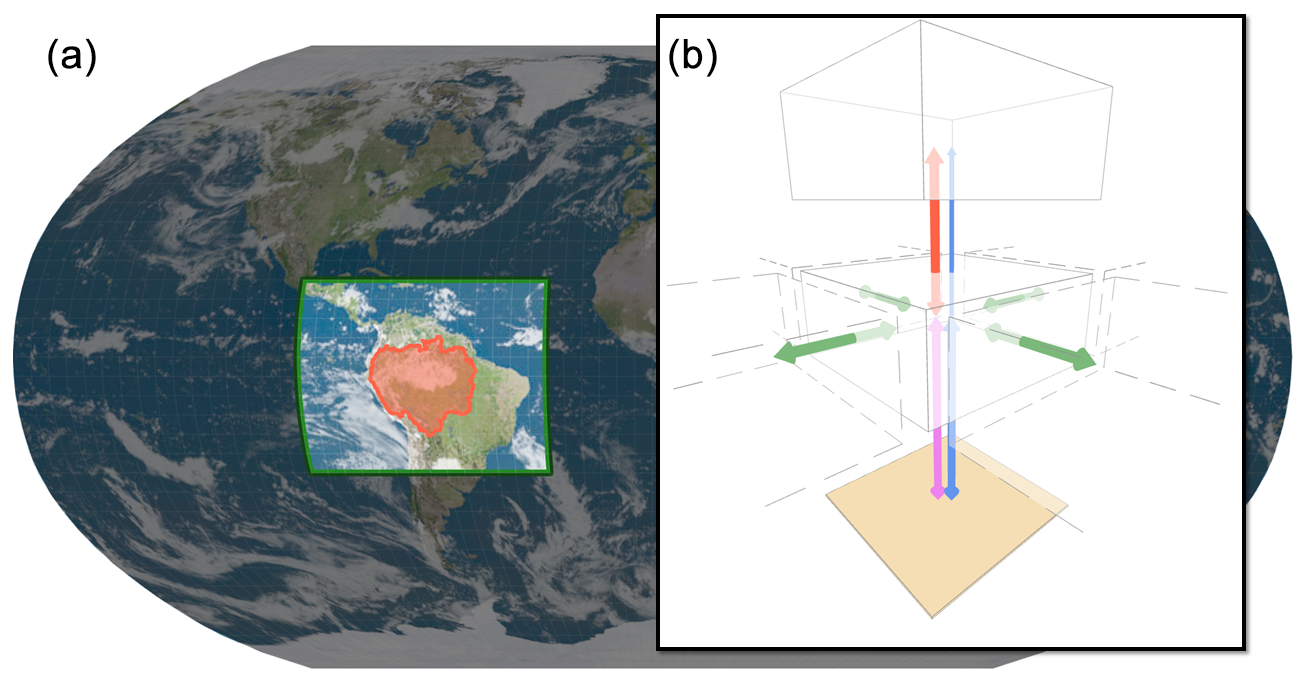
Figure 1 (a) Example tracking domain (green outline) and tagging region (red outline and shading) for WAM2layers overlaid on a global input grid. (b) Conceptual illustration of the inner structure of WAM2layers. Green arrows indicate horizontal transport, the red arrow indicates the vertical flux, the blue arrow indicates precipitation, and the purple arrow indicates evaporation. Horizontal transport in the upper layer (not drawn) is similar to that in the lower layer. The yellow square represents the surface.

WAM2layers was originally developed as the single-layer Water Accounting Model (WAM v1; Van der Ent et al., 2010), driven by ERA-Interim data. The two-layer version was introduced because Van der Ent et al. (2013), who compared the capabilities of WAM to an online tracking method in a regional climate model, found that the one-layer version resulted in large errors for cases with strong directional wind shear. After further adjustments for use with global climate and reanalysis data, the version described in Van der Ent et al. (2014, their Appendix B) is referred to as WAM2layers v1. Originally written in MATLAB, the first published work with a full rewrite into Python was by Van der Ent and Tuinenburg (2017) (WAM2layers v2). Hence, the update to the model described here is considered to be WAM2layers v3. This major rewrite was aimed at improving the code efficiency in order to keep up with the increased resolution of weather and climate model output. As of v3, we started using semantic versioning (https://semver.org/, last access: 14 July 2025), which means each software release gets a three-number identifier using the following format: major.minor.patch. Within a major version, we strive to maintain backward compatibility, minimizing disruptions to existing workflows with WAM2layers as new features and fixes are introduced. This paper pertains to major version v3, including all of its minor and patch releases. Each release gets its own DOI to enable the referencing of specific versions of the code. Additionally, a concept DOI is available for generic references to the software regardless of a specific version (Van der Ent et al., 2024a).

Since its introduction, WAM2layers has been used by many researchers and applied to different topics (Table 1). Figure 2 shows a breakdown of use cases by time and data source. The use of WAM2layers has increased over time, and the model has predominantly been used with reanalysis data, although it has sometimes also been employed with climate model output. Studies that have used the output data from WAM2layers for further analysis (Al Hasan et al., 2021; Berger et al., 2014, 2018; Cui et al., 2022; Link et al., 2021; Van der Ent and Savenije, 2011; Weng et al., 2019) are not included in this overview (Table 1, Fig. 2).

Bedoya‐Soto and Poveda (2024); Enciso et al. (2022); Keys et al. (2014, 2024); Posada‐Marín et al. (2023); Shi et al. (2022); Van der Ent et al. (2010); Zemp et al. (2014); Zhang et al. (2020)Carr and Ummenhofer (2024); Chen et al. (2023); Cluett et al. (2021); Guo et al. (2019); Li et al. (2021, 2022); Link et al. (2020); Lobos-Roco et al. (2022); Mu et al. (2023); Van der Ent and Savenije (2013); Van der Ent and Tuinenburg (2017); Xia et al. (2022); Xiao and Cui (2021); Zhang (2020b); Zhao et al. (2016)Keys et al. (2017); Keys and Wang-Erlandsson (2018); Keys et al. (2018); Posada-Marín et al. (2024)Ampuero et al. (2020); Duerinck et al. (2016); Keys et al. (2016, 2022); Van der Ent et al. (2012, 2014)De Hertog et al. (2024); Keys et al. (2012); Li et al. (2017); Wang-Erlandsson et al. (2018); Zemp et al. (2017)Bosmans et al. (2020)Franco-Díaz et al. (2024); Guo et al. (2020)Benedict et al. (2020); Findell et al. (2019); Liu et al. (2022, 2024); Yuan et al. (2023a); Zhang et al. (2019, 2023a, b)Benedict et al. (2021); Mu et al. (2021); Pranindita et al. (2022); Zhang (2020a); Zhou and Shi (2024)Liu et al. (2021); Yuan et al. (2023b); Zhang et al. (2023b, 2024)Li et al. (2024); Van der Ent et al. (2013)

Table 1 Topics for which WAM2layers has been used and associated references to work on these topics.

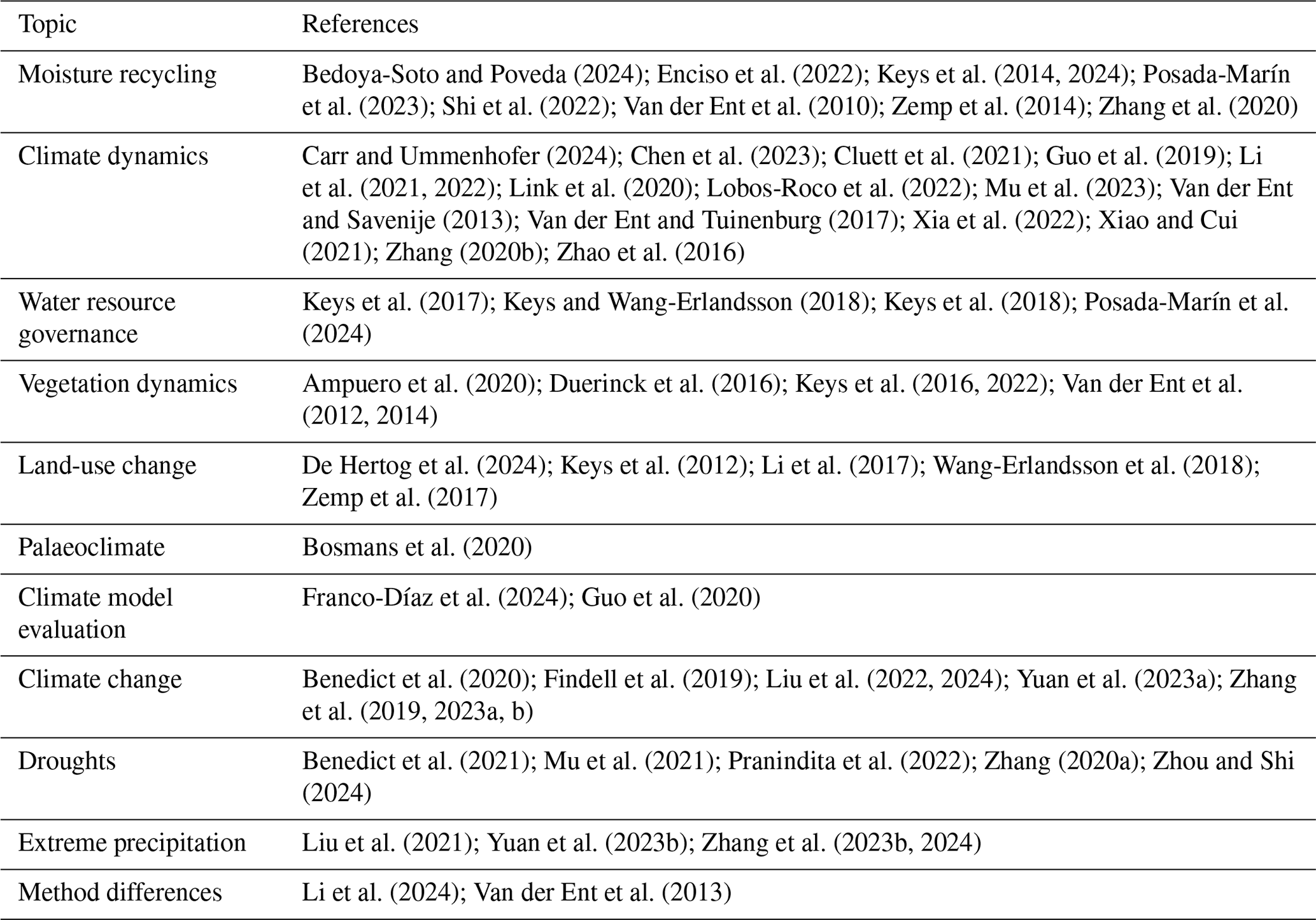
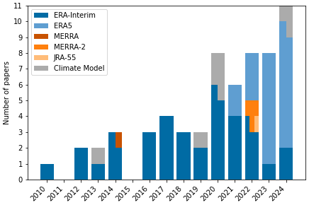
Figure 2 Peer-reviewed scientific papers running WAM2layers (or its predecessor WAM) as of 30 September 2024. The data source only refers to the atmospheric wind and humidity fields, as some studies used evaporation or precipitation from other data sources. The “Climate Model” category groups different models. The underlying data are provided in the Supplement.

Evidently, WAM2layers has developed into a mature piece of research software with a considerable user base. We envision that this reference paper will (1) help to run it consciously with appropriate model settings to interpret existing results and (2) serve as a sound basis for future model improvements and sensitivity studies to understand the effects of certain modelling decisions in detail. The governing equations are derived in Sect. 2. Section 3 describes the preprocessing procedure, i.e. how to prepare data from various sources for a tracking experiment. Section 4 describes the actual tracking procedure. In Sect. 5, we briefly discuss two reference cases. Section 6 is dedicated to the best practices that have been incorporated in WAM2layers. Strengths, weaknesses, and opportunities for future development are discussed in Sect. 7.

2 Governing equations

Here, we describe the budget equations for total and tagged moisture as they are implemented in WAM2layers v3. To facilitate comparison with other (moisture-tracking or tracer) models, we present a generic description that extends to more than two layers. The two-layer concept will emerge more clearly in Sects. 3 and 4, where we describe in detail how the input data are collapsed from an arbitrary number of model or pressure levels onto a two-layer grid, and how the equations are implemented numerically.

2.1 Total moisture budget

As the name “Water Accounting Model” implies, WAM2layers is primarily concerned with bookkeeping the amount of water that is exchanged between grid cells. The total water vapour S per unit area 𝒜 contained in a 3D grid cell of volume 𝒱=𝒜Δz is calculated as follows:

$$\begin{array}{}\text{(1)}& S={\displaystyle \frac{\mathrm{1}}{\mathcal{A}}}\underset{\mathcal{V}}{\int }q\mathit{\rho }\mathrm{d}\mathcal{V}=q\mathit{\rho }\mathrm{\Delta }z={\displaystyle \frac{q\mathrm{\Delta }p}{g}},\end{array}$$

where q is the specific humidity, ρ is the density of the air, g is the gravitational constant, and p is pressure. The change from height to pressure coordinates is accomplished through substitution of hydrostatic balance, which conveniently eliminates the density. Changes in grid cell area with height are neglected. Notice that WAM2layers uses specific humidity as a proxy for specific water content. As discussed in Sect. 3, it is possible to account for other phases of water to some extent by using the total column water, if this variable is available in the input data.

The area-averaged moisture content is convenient to work with, as the corresponding unit of kilograms per square metre (kg m⁻²) is commonly used and allows for straightforward interpretation of the values of the moisture fields. Older versions of WAM2layers have worked with $\frac{\left(S\mathcal{A}\right)}{{\mathit{\rho }}_{\mathrm{lw}}}$ instead, where ρ_lw represents the density of liquid water, thereby effectively working in units of cubic metres (m³). While the moisture balance is not affected, the input and output of WAM2layers are different between v3 and older versions.

As the total moisture is a conserved quantity, the change in (area-averaged) moisture S in a grid cell is equal to the fluxes through the boundary of the grid cell plus the sources and sinks:

$$\begin{array}{}\text{(2)}& {\displaystyle \frac{{\mathrm{\Delta }}_{t}S}{\mathrm{\Delta }t}}+{\displaystyle \frac{\mathrm{1}}{\mathcal{A}}}\left({\mathrm{\Delta }}_x{F}_x+{\mathrm{\Delta }}_y{F}_y+{\mathrm{\Delta }}_{\mathrm{p}}{F}_{\mathrm{p}}\right)=E-P,\end{array}$$

where the terms on the left-hand side represent the change in moisture in a grid cell and the horizontal (green arrows in Fig. 1b) and vertical (red arrow) fluxes, respectively. The terms on the right-hand side represent the rates of removal by precipitation (P, blue arrow) and addition through evaporation (E, purple arrow), both per unit area. Considering advection as the main mode of transport, the horizontal fluxes between grid cells are given by the following:

$$\begin{array}{}\text{(3)}& {\displaystyle }{F}_x={\displaystyle \frac{uq\mathrm{\Delta }y\mathrm{\Delta }p}{g}},F_y={\displaystyle \frac{vq\mathrm{\Delta }x\mathrm{\Delta }p}{g}},\end{array}$$

where u and v are the zonal and meridional wind components, respectively. For our two-layer model, the vertical fluxes F_p at the top and bottom boundaries vanish, leaving only one vertical transport term at the interface between the two layers. As the vertical flux is positive downwards, this term acts as a sink for the top layer and as a source for the bottom layer. Importantly, this vertical transport term is ill-defined. Advection is typically not the main process for vertical transport. Unresolved processes, such as convection and transport associated with precipitation, can also lead to a strong vertical redistribution of water. Another complicating factor is that the vertical extent of the grid cells may vary in time and space. Therefore, in solving for Eq. (2), all terms are estimated from the input data (see Sect. 3), except for the vertical transport, which is calculated as a closure term (see Sect. 4).

2.2 Tagged moisture budget

The core of WAM2layers consists of tracking a certain proportion of the total moisture, which we refer to as “tagged” moisture. We define the tagged moisture contained in a grid cell as follows:

$$\begin{array}{}\text{(4)}& S^{*}=cS,\end{array}$$

where c represents the tagged moisture concentration. Seeking a budget equation for S^*, we recast Eq. (2) in terms of tagged moisture:

$$\begin{array}{}\text{(5)}& {\displaystyle \frac{{\mathrm{\Delta }}_t{S}^{*}}{\mathrm{\Delta }t}}+{\displaystyle \frac{\mathrm{1}}{\mathcal{A}}}\left({\mathrm{\Delta }}_x{F}_x^{*}+{\mathrm{\Delta }}_y{F}_y^{*}+{\mathrm{\Delta }}_{\mathrm{p}}{F}_{\mathrm{p}}^{*}\right)=E^{*}-P^{*}\end{array}$$

such that tagged moisture transport is described by the same fluxes as the total moisture (illustrated in Fig. 1b), except that tagged moisture represents only a portion of the total.

As opposed to Eq. (2), which is complete in terms of the input data, Eq. (5) is incomplete and must be modelled. Thus, our quest is to express the unknown fluxes of tagged moisture, denoted by asterisks, as a function of the known terms of the total moisture budget. For the sources and sinks we write the following:

$$\begin{array}{}\text{(6)}& {\displaystyle }{E}^{*}& {\displaystyle }={\mathit{\delta }}_{\mathrm{e}}E,\text{(7)}& {\displaystyle }{P}^{*}& {\displaystyle }={\mathit{\delta }}_{\mathrm{p}}P.\end{array}$$

Here, δ_e and δ_p control where water is added or removed from the system. This is controlled by the tagging region, marked by the red outline and fill in Fig. 1a. In the case of forward tracking, δ_e is 1 inside the tagging (source) region and 0 elsewhere, and δ_p=c; i.e. precipitation is removed proportionally to the total moisture in the upper and lower layer. For backward tracking, it is the exact opposite: δ_p is 1 inside the tagging (sink) region and 0 elsewhere, and δ_e=c; i.e. evaporation is removed proportionally from the lower layer. For the fluxes, WAM2layers uses the following:

$$\begin{array}{}\text{(8)}& F_x^{*}=c{F}_x,F_y^{*}=c{F}_y,F_{\mathrm{p}}^{*}=c{F}_{\mathrm{p}}+\mathit{\kappa }{\displaystyle \frac{{\mathrm{\Delta }}_{\mathrm{p}}c}{\mathrm{\Delta }p}};\end{array}$$

that is, tagged moisture transport is proportional to the transport of total moisture in the horizontal direction. In the vertical, an additional dispersion term is added, as Van der Ent et al. (2014) noticed that there was insufficient vertical mixing of tagged moisture without it. Setting $\mathit{\kappa }=k_{\mathrm{vf}}\left|F_{\mathrm{p}}\right|\mathrm{\Delta }p$ ensures that the dispersion rate is proportional to vertical advection rate F_p and the grid size. A similar form may be found in Cushman-Roisin and Beckers (2011, p. 138), who reason that κ is characterized by the largest unresolved eddies. Here, k_vf is a tunable parameter to control the dispersion rate. Van der Ent et al. (2014) suggested that a value of 3 gives realistic results, but this could be case-dependent.

2.3 Some notes on the formulation of WAM2layers

Although originally conceived as a simple bookkeeping exercise, the accounting method in WAM2layers has a formal basis in the finite-volume approach. In the absence of sources and sinks, conservation of moisture reads as follows:

$$\begin{array}{}\text{(9)}& {\displaystyle \frac{\partial \left(\mathit{\rho }q\right)}{\partial t}}+\mathrm{\nabla }\cdot \mathit{f}\left(\mathit{\rho }q\right)=\mathrm{0},\end{array}$$

where f(x) represents a generic flux function (for advection only, f(x)=ux). Integrating all terms over a fixed control volume and applying Gauss' theorem to the divergence term yields an equivalent expression, stating that the rate of change in moisture in a grid cell is equivalent to the flux across its enclosing surface. Upon discretization, substitution of hydrostatic balance, and division by the grid cell area, we retrieve Eq. (2). Applying this procedure to grid cells with a variable vertical extent rather than a fixed control volume yields an additional term by virtue of the Leibniz rule. This term is effectively “absorbed” by our loose definition of the vertical flux.

On a Cartesian grid with 𝒜=ΔxΔy, the horizontal transport in Eq. (2) can be written as ∇⋅F using the following expression:

$$\begin{array}{}\text{(10)}& \mathit{F}=(F_x,F_y)=\left({\displaystyle \frac{uq\mathrm{\Delta }p}{g}},{\displaystyle \frac{vq\mathrm{\Delta }p}{g}}\right).\end{array}$$

This testifies to the equivalence of the continuous and integrated budget equations. However, as WAM2layers operates on a spherical latitude–longitude grid, we must stick with Eq. (2) to ensure that meridional transport is dependent on latitude.

To facilitate numerical stability analysis and comparison to other moisture-tracking methods and, more broadly, to tracer models in general, it is convenient to define an “integrated moisture velocity” $\widehat{\mathit{u}}=(\widehat{u},\widehat{v},\widehat{\mathit{\omega }})$ such that

$$\begin{array}{}\text{(11)}& F_x=\widehat{u}S,F_y=\widehat{v}S,F_{\mathrm{p}}=\widehat{\mathit{\omega }}S.\end{array}$$

With this, conservation of total moisture, tagged moisture, and tagged moisture concentration can all be expressed in the same form:

$$\begin{array}{}\text{(12)}& {\displaystyle \frac{\partial S}{\partial t}}+\mathrm{\nabla }\cdot \left(\widehat{\mathit{u}}S\right)=\mathrm{0},\text{(13)}& {\displaystyle \frac{\partial S^{*}}{\partial t}}+\mathrm{\nabla }\cdot \left(\widehat{\mathit{u}}{S}^{*}\right)=\mathrm{0},\text{(14)}& {\displaystyle \frac{\partial c}{\partial t}}+\mathrm{\nabla }\cdot \left(\widehat{\mathit{u}}c\right)=\mathrm{0}.\end{array}$$

In relation to existing literature, we point out that Trenberth and Guillemot (1995), Dominguez et al. (2006), and Burde and Zangvil (2001) take a slightly different approach to calculate integrated vapour transport. They take the vertical integral of each term in Eq. (9) in isobaric coordinates and apply the Leibniz rule to each of the terms, upon which the vertical flux disappears from the budget equation. In their case, as they consider the budget equation vertically integrated over the full atmosphere, this makes perfect sense. In our case, as mentioned before, we need to retain a vertical transport term between the two layers of our model, due to unresolved and non-isobaric processes, and variability in the grid cells' vertical extent. Note that the aforementioned studies used the symbol w (sometimes referred to as “precipitable water”) for what we refer to as the total moisture S.

2.4 Summary

Recapitulating, the heart of WAM2layers consists of Eqs. (2) and (5) for total moisture S and tagged moisture S^*, respectively. These governing equations naturally lead to a two-step process for using WAM2layers. First, the input data are collapsed onto a two-layer grid, and the terms in Eq. (2) are reconstructed from the available input data. This is what we refer to as the preprocessing step. Subsequently, Eq. (5) is integrated numerically, which we call the tracking step. In the next sections, we will discuss each of these steps in detail.

3 Preprocessing

The first step in any WAM2layers experiment is to collapse the input data onto a two-layer grid and to reconstruct the corresponding terms in Eq. (2) for each new grid cell, except for the vertical flux, which will be calculated as a closure term later on. This procedure is dataset-dependent; therefore, it is isolated from the rest of the code in a dedicated preprocessing module. This makes it possible to support multiple input datasets with minimal code duplication.

In developing WAM2layers v3, we have primarily focused on working with ERA5 reanalysis data (Hersbach et al., 2020). The comprehensiveness of this dataset enables scrutiny in the treatment of vertical levels, which also facilitates the presentation in this paper. We aim for a complete description such that a similar procedure can easily be derived for other data sources.

3.1 Data retrieval: required variables

ERA5 data can be downloaded at model levels or pressure levels. In either case, the forthcoming steps require the horizontal wind components (u and v) and specific humidity (q) as input at all or a subset of the available levels. Furthermore, precipitation (P), evaporation (E), and surface pressure (p_s) are required at the surface, and we also include total column water (S_{tc_ERA5}). This last variable is not strictly required to run WAM2layers, but it enables us to estimate and mitigate (to some extent) the errors introduced by the omission of liquid and ice water. Working with pressure-level data additionally requires the surface values of wind and humidity, i.e. the 10 m wind components u₁₀ and v₁₀ and 2 m dew point temperature T_d,2. While ERA5 data are available globally, WAM2layers can be configured to use only a subset of the data. This can be useful to speed up data downloads and simulations or to reduce disc space requirements. The domain at which WAM2layers operates is referred to as the “tracking domain” (Fig. 1a), and it can be provided as a bounding box or as a 2D raster to allow for arbitrary regions.

3.2 States and fluxes

We start by describing the ideal case in which the 3D fields of u, v, and q are available on all model levels. WAM2layers aggregates the input data onto a two-layer grid by partitioning the input grid into an upper (k=0) and lower (k=1) part and then taking the sum over each layer.

Summation of Eq. (1) over each partition k gives the total water in each grid cell in WAM2layers:

$$\begin{array}{}\text{(15)}& S_k={\displaystyle \frac{\mathrm{1}}{g}}\sum _{i\in k}{q}_i\mathrm{\Delta }{p}_i.\end{array}$$

Here, the subscript i refers to indices in the ERA5 level definition, which can be found in the documentation of the underlying Integrated Forecasting System (IFS) (ECMWF, 2016). Horizontal advection terms are calculated according to Eq. (3) and then aggregated in a similar fashion:

$$\begin{array}{}\text{(16)}& F_{x,k}={\displaystyle \frac{\mathrm{1}}{g}}\sum _{i\in k}{u}_i{q}_i\mathrm{\Delta }{p}_i,F_{y,k}={\displaystyle \frac{\mathrm{1}}{g}}\sum _{i\in k}{v}_i{q}_i\mathrm{\Delta }{p}_i.\end{array}$$

Following Van der Ent et al. (2013, 2014), we set the boundary to be at the interface between IFS levels 111 and 112 by default. This corresponds to around 812 hPa, for a standard atmospheric pressure of 1013.25 hPa. This boundary in WAM2layers is usually just above the atmospheric boundary layer with, on average, slightly more moisture below the boundary than above the boundary. Note that the boundary can be at a much lower pressure over mountainous terrain.

The vertical pressure difference over each input grid cell can be calculated as follows:

$$\begin{array}{}\text{(17)}& {\displaystyle }\mathrm{\Delta }{p}_i=p_{i+\mathrm{1}/\mathrm{2}}-p_{i-\mathrm{1}/\mathrm{2}},\text{(18)}& {\displaystyle }{p}_{i+\mathrm{1}/\mathrm{2}}=A_{i+\mathrm{1}/\mathrm{2}}+p_{s,i+\mathrm{1}/\mathrm{2}}B,\end{array}$$

where A and B are hybrid model level coefficients describing the vertical discretization of the model levels in IFS (ECMWF, 2016).

Accounting for liquid and solid water

Equation (15) represents the total mass of water vapour in each grid cell. By contrasting the calculated column water vapour with the total column water from ERA5 (S_{T_ERA5}), we can apply an adjustment to account for other phases of water:

$$\begin{array}{}\text{(19)}& S_k=S_k{\displaystyle \frac{S_{\mathrm{T}\mathrm{\_}\mathrm{ERA}\mathrm{5}}}{{\sum }_k{S}_k}}.\end{array}$$

This adds missing cloud and rain/snow water to all levels proportionally to the vertical distribution of water vapour. For the two example cases, this correction is typically within 1 % when averaged over the grid, although it may be more than 10 % for specific individual grid cells and time steps. WAM2layers provides information about this in the on-screen logging and associated log file. Note that this step is only possible when the total column water is available from the input data source, which is not always the case.

3.3 Sources and sinks

In the formulation of WAM2layers's equations, we adopted the common convention in hydrology of having only positive values for both precipitation and evaporation. Precipitation represents all water transfer from the atmosphere to the surface, including condensation.

In ERA5, vertical fluxes are defined positive downwards. The evaporation variable can be either positive (condensation) or negative (evaporation). Therefore, during the preprocessing step for ERA5, the sign of evaporation is flipped and any remaining negative values are reassigned to the precipitation variable instead.

In a forward-tracking experiment, a proportion of the total surface evaporation is tagged (δ_e). Similarly, for a backward-tracking experiment, we tag a proportion of the precipitation (δ_p). The tagging region is illustrated in Fig. 1a. It can be supplied as a bounding box or as a 2D/3D raster. The 3D option, which is still relatively experimental, would allow for a moving tagging region, e.g. for studying storms. In the 2D case, a tagging start date and end date are given in the configuration file.

3.4 Dealing with fewer model levels

ERA5 data are available at all 137 model levels, which is quite unique in terms of resolution (Hersbach et al., 2020) but also quite demanding in terms of storage and processing. As we collapse the data onto a two-layer grid anyway, it is not necessary to use all 137 levels. To use WAM2layers with only a subset of these 137 layers, A and B in Eq. (18) are first interpolated to the full levels of the layer subset and then to the interfaces between these full levels. This procedure is illustrated in Fig. 3.

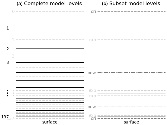
Figure 3 Illustration of how WAM2layers treats a subset of layers. Full black lines are full levels, whereas dashed grey lines are half-levels. In panel (b), the top and bottom half-levels are retained, but the remaining half-levels are expired. New half-levels are obtained by interpolating between the selected full levels.

Based on our experience with a few test cases, around 20 layers gives good results, provided that the sampling is dense enough near the surface where most of the moisture is located. However, the number of input levels is configurable, so users of WAM2layers are encouraged to experiment with different subsets as they see fit.

3.5 Working with pressure-level data

Working with (a limited number of) pressure levels instead of model levels is sometimes the only option. This is, for example, the case for datasets from Coupled Model Intercomparison Project (CMIP) archives (Juckes et al., 2020, Table 4). ERA5 data are also available on pressure levels, and WAM2layers v3 provides code to work with pressure-level data as well.

From the point of view of achieving accurate moisture tracking, having wind and humidity data near the surface is crucial, but these data could be absent in the case of limited pressure levels. Therefore, in order to work with (ERA5) pressure-level data, we complement the data with additional values from the surface-level data (2 m specific humidity and 10 m wind), as these are generally more representative of the surface conditions than the closest available pressure level. In addition, at the top of the atmosphere, WAM2layers assumes humidity to be zero and wind to be equal to the pressure level with the lowest pressure. This procedure is illustrated in Fig. 4.

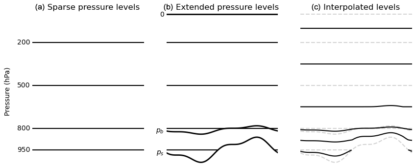
Figure 4 Pressure-level data preprocessing. Panel (a) presents the original pressure levels. In panel (b), the original levels are extended at the top and surface and the interface is inserted. In panel (c), wind and humidity are interpolated to the midpoints between the pressure coordinate to become the new full levels (full black lines). Pressure is kept at the original levels, which thus become the new half-levels (dashed grey lines).

The surface pressure is used to insert these values in between the right pressure levels. As surface pressure is spatially and temporally dependent ($p_{\mathrm{s}}=p_{\mathrm{s}}(x,y,t)$), the same now applies to our vertical coordinate: $p=p(x,y,z,t)$. A further complication is that the pressure levels can intersect the surface, so we mask any data for which the pressure is higher than the surface pressure.

The interface between the two layers in WAM2layers must also follow the terrain. For consistency with the treatment of model-level data, we define the interface according to Eq. (18). By default, we use the A and B values for level IFS 111; however, this is configurable since WAM2layers v3.1, and users of WAM2layers can therefore easily modify it as they see fit.

At this point, the variables of interest, wind speed and humidity, are co-located with the pressure coordinate. To calculate the grid cell moisture content and fluxes, we need to multiply the pressure difference over a volume with representative values for that same volume. Thus, we interpolate wind and humidity to the interfaces between the pressure coordinates. Finally, we can proceed with evaluating Eqs. (15) and (16) as before.

3.6 Preprocessing other datasets

WAM2layers is set up in such a way that it is relatively easy to extend its preprocessing to any dataset. Most of the steps outlined above are implemented as generic routines that can be used for any dataset. To add a dataset, only a data loader script has to be implemented, which loads data into a standard internal format. As of version 3.2, built-in preprocessing is available for ERA5 data (on both model levels and pressure levels) and for CMIP data (on pressure levels). We also support ERA5 pressure-level data from ARCO-ERA5 (Carver and Merose, 2023). We envision that more datasets will be included in the future, and we foster community contributions such that other researchers can also contribute their own custom preprocessing scripts.

4 Tracking

The preprocessing step is designed in such a way that the intermediate data can be stored efficiently. As part of the tracking routine, the data are first interpolated to a finer time step (∼ 10 min; see Sect. 4.3), after which we solve for the vertical transport term in Eq. (2). Finally, Eq. (5) is integrated numerically.

4.1 Solving for the vertical flux

In discretizing Eq. (2), we assign the full evaporation source to the lower layer, but we distribute the precipitation sink proportionally over both layers. Additionally, we introduce an error term to account for inaccuracies, numerical errors, and inconsistencies in the input data caused by both the raw (ERA5) data as well as the preprocessing in WAM2layers. This leads to the following, fully discretized system of equations:

$$\begin{array}{}\text{(20)}& \begin{array}{rl}{\displaystyle \frac{S_{ijk}^{t+\mathrm{1}}-S_{ijk}^t}{\mathrm{\Delta }t}}& +(F_{x,i+\frac{\mathrm{1}}{\mathrm{2}}jk}-F_{x,i-\frac{\mathrm{1}}{\mathrm{2}}jk})/{\mathcal{A}}_j\\ & +(F_{y,ij+\frac{\mathrm{1}}{\mathrm{2}}k}-F_{y,ij-\frac{\mathrm{1}}{\mathrm{2}}k})/{\mathcal{A}}_j\\ & +(F_{\mathrm{p},ijk+\frac{\mathrm{1}}{\mathrm{2}}}-F_{\mathrm{p},ijk-\frac{\mathrm{1}}{\mathrm{2}}})/{\mathcal{A}}_j\\ & ={\mathit{\delta }}_k{E}_{ij}-{\displaystyle \frac{S_{ijk}}{S_{ij\mathrm{T}}}}{P}_{ij}+{\mathit{ϵ}}_{ijk}^{t+\mathrm{1}}.\end{array}\end{array}$$

Here all fluxes are evaluated at $t+\frac{\mathrm{1}}{\mathrm{2}}$; the superscripts are omitted for clarity; S_ijT represents the calculated column total, whether or not corrected for cloud/rain/snow water as per Eq. (19); and δ_k is 1 for the lower layer (k=1) and 0 otherwise. Note that, in Eq. (20), the vertical flux is positive downward in accordance with the pressure coordinate. For convenience, we can move all known terms to the left-hand side and all unknowns to the right. Using R to denote the known terms and leaving out the subscripts i,j for clarity, we get

$$\begin{array}{}\text{(21)}& R_k=-(F_{\mathrm{p},k+\frac{\mathrm{1}}{\mathrm{2}}}-F_{\mathrm{p},k-\frac{\mathrm{1}}{\mathrm{2}}})/\mathcal{A}+{\mathit{ϵ}}_k.\end{array}$$

After applying the boundary conditions F_p=0 at the bottom and top, the only remaining net vertical flux in our two-layer model is at the interface $F_{\mathrm{p}}=F_{\mathrm{p},\frac{\mathrm{1}}{\mathrm{2}}}$, such that

$$\begin{array}{}\text{(22)}& R_{\mathrm{0}}=-{\displaystyle \frac{F_{\mathrm{p},\frac{\mathrm{1}}{\mathrm{2}}}}{\mathcal{A}}}+{\mathit{ϵ}}_{\mathrm{0}},R_{\mathrm{1}}=+{\displaystyle \frac{F_{\mathrm{p},\frac{\mathrm{1}}{\mathrm{2}}}}{\mathcal{A}}}+{\mathit{ϵ}}_{\mathrm{1}}.\end{array}$$

To solve this system, we introduce another constraint by requiring that the errors are proportionally distributed between the upper and lower layer:

$$\begin{array}{}\text{(23)}& {\displaystyle \frac{{\mathit{ϵ}}_k}{{\mathit{ϵ}}_{\mathrm{T}}}}={\displaystyle \frac{S_k}{S_{\mathrm{T}}}}.\end{array}$$

Isolating ϵ_k and recognizing that the total error should be equal to the total residual, we have

$$\begin{array}{}\text{(24)}& {\mathit{ϵ}}_k={\displaystyle \frac{{\mathit{ϵ}}_{\mathrm{T}}{S}_k}{S_{\mathrm{T}}}}={\displaystyle \frac{R_{\mathrm{T}}{S}_k}{S_{\mathrm{T}}}}.\end{array}$$

Substituting this result in Eq. (22) we finally arrive at

$$\begin{array}{}\text{(25)}& {\displaystyle \frac{F_{\mathrm{p},\frac{\mathrm{1}}{\mathrm{2}}}}{\mathcal{A}}}=-R_{\mathrm{0}}+{\displaystyle \frac{R_{\mathrm{T}}{S}_{\mathrm{0}}}{S_{\mathrm{T}}}}=R_{\mathrm{1}}-{\displaystyle \frac{R_{\mathrm{T}}{S}_{\mathrm{1}}}{S_{\mathrm{T}}}}.\end{array}$$

In the software implementation, as well as in previous publications, this term $F_{\mathrm{p},\frac{\mathrm{1}}{\mathrm{2}}}/\mathcal{A}$ is typically simply referred to as “the vertical flux”, F_v.

4.2 Numerical integration

The formulation of WAM2layers naturally lends itself to a finite-volume implementation, where the incoming fluxes in one cell correspond to outgoing fluxes in its neighbours. Concretely, in the case of forward tracking, we have the following for the upper and lower layers, respectively:

$$\begin{array}{}\text{(26)}& {\displaystyle }\begin{array}{rl}{S}_{ij\mathrm{0}}^{t+\mathrm{1}}& =S_{ij\mathrm{0}}^t+\mathrm{\Delta }t[\\ & -(F_{x,i+\mathrm{1}/\mathrm{2},j\mathrm{0}}^{*}-F_{x,i-\mathrm{1}/\mathrm{2},j\mathrm{0}}^{*})/\mathcal{A}\\ & -(F_{y,i,j+\mathrm{1}/\mathrm{2},\mathrm{0}}^{*}-F_{y,i,j-\mathrm{1}/\mathrm{2},\mathrm{0}}^{*})/\mathcal{A}\\ & -(F_{\mathrm{p},ij,\mathrm{1}/\mathrm{2}}^{*}+k_{\mathrm{vf}}|F_{\mathrm{p},ij,\mathrm{1}/\mathrm{2}}\left|\right(c_{ij,\mathrm{1}}^t-c_{ij\mathrm{0}}^t\left)\right)/\mathcal{A}\\ & -c_{ij\mathrm{0}}{\displaystyle \frac{S_{ij\mathrm{0}}}{S_{ij\mathrm{T}}}}{P}_{ij}^{t+\mathrm{1}/\mathrm{2}}],\end{array}\text{(27)}& {\displaystyle }\begin{array}{rl}{S}_{ij\mathrm{1}}^{t+\mathrm{1}}& =S_{ij\mathrm{1}}^t+\mathrm{\Delta }t[\\ & -(F_{x,i+\mathrm{1}/\mathrm{2},j\mathrm{1}}^{*}-F_{x,i-\mathrm{1}/\mathrm{2},j\mathrm{1}}^{*})/\mathcal{A}\\ & -(F_{y,i,j+\mathrm{1}/\mathrm{2},\mathrm{1}}^{*}-F_{y,i,j-\mathrm{1}/\mathrm{2},\mathrm{1}}^{*})/\mathcal{A}\\ & +(F_{\mathrm{p},ij,\mathrm{1}/\mathrm{2}}^{*}+k_{\mathrm{vf}}|F_{\mathrm{p}}\left|\right(c_{ij,\mathrm{1}}^t-c_{ij\mathrm{0}}^t\left)\right)/\mathcal{A}\\ & +{\mathit{\delta }}_{\mathrm{e}}{E}_{ij}^{t+\mathrm{1}/\mathrm{2}}-c_{ij\mathrm{1}}{\displaystyle \frac{S_{ij\mathrm{1}}}{S_{ij\mathrm{T}}}}{P}_{ij}^{t+\mathrm{1}/\mathrm{2}}].\end{array}\end{array}$$

Note that the only remaining vertical transport term, which is shared by both equations, is directed from the upper to the lower layer. δ_e is the tagging region (see Sect. 3).

A crucial aspect of any finite-volume scheme is how the fluxes at the interfaces are calculated. WAM2layers employs a simple donor cell scheme (see e.g. Cushman-Roisin and Beckers, 2011). In this scheme, the flux of tagged moisture $F^{*}=cF$ is constructed by combining F, calculated at the interfaces of the grid cell and at $t+\mathrm{1}/\mathrm{2}$, with c at t, taken from the upstream volume. Concretely,

$$\begin{array}{}\text{(28)}& (cF{)}_{{}_x,i+\mathrm{1}/\mathrm{2}jk}=\left\{\begin{array}{ll}{F}_{x,i+\mathrm{1}/\mathrm{2}jk}^{t+\mathrm{1}/\mathrm{2}}{c}_{ijk}^t,& \text{if }{F}_{x,i+\mathrm{1}/\mathrm{2}jk}^{t+\mathrm{1}/\mathrm{2}}>\mathrm{0}\\ F_{x,i+\mathrm{1}/\mathrm{2}jk}^{t+\mathrm{1}/\mathrm{2}}{c}_{i+\mathrm{1}jk}^t,& \text{otherwise}\end{array}\right.\end{array}$$

and similarly for the other directions.

In case of backward tracking, the equations are similar:

$$\begin{array}{}\text{(29)}& {\displaystyle }\begin{array}{rl}{S}_{ij\mathrm{0}}^{t-\mathrm{1}}& =S_{ij\mathrm{0}}^t-\mathrm{\Delta }t[\\ & -(F_{x,i+\mathrm{1}/\mathrm{2},j\mathrm{0}}^{*}-F_{x,i-\mathrm{1}/\mathrm{2},j\mathrm{0}}^{*})/\mathcal{A}\\ & -(F_{y,i,j+\mathrm{1}/\mathrm{2},\mathrm{0}}^{*}-F_{y,i,j-\mathrm{1}/\mathrm{2},\mathrm{0}}^{*})/\mathcal{A}\\ & -(F_{\mathrm{p},ij,\mathrm{1}/\mathrm{2}}^{*}+k_{\mathrm{vf}}|F_{\mathrm{p}}\left|\right(c_{ij,\mathrm{1}}^t-c_{ij\mathrm{0}}^t\left)\right)/\mathcal{A}\\ & -{\mathit{\delta }}_{\mathrm{p}}{\displaystyle \frac{S_{ij\mathrm{0}}}{S_{ij\mathrm{T}}}}{P}_{ij}^{t-\mathrm{1}/\mathrm{2}}],\end{array}\text{(30)}& {\displaystyle }\begin{array}{rl}{S}_{ij\mathrm{1}}^{t-\mathrm{1}}& =S_{ij\mathrm{1}}^t-\mathrm{\Delta }t[\\ & -(F_{x,i+\mathrm{1}/\mathrm{2},j\mathrm{1}}^{*}-F_{x,i-\mathrm{1}/\mathrm{2},j\mathrm{1}}^{*})/\mathcal{A}\\ & -(F_{y,i,j+\mathrm{1}/\mathrm{2},\mathrm{1}}^{*}-F_{y,i,j-\mathrm{1}/\mathrm{2},\mathrm{1}}^{*})/\mathcal{A}\\ & +(F_{\mathrm{p},ij,\mathrm{1}/\mathrm{2}}^{*}+k_{\mathrm{vf}}|F_{\mathrm{p}}\left|\right(c_{ij,\mathrm{1}}^t-c_{ij\mathrm{0}}^t\left)\right)/\mathcal{A}\\ & +c_{ij\mathrm{1}}{E}_{ij}^{t-\mathrm{1}/\mathrm{2}}-{\mathit{\delta }}_{\mathrm{p}}{\displaystyle \frac{S_{ij\mathrm{1}}}{S_{ij\mathrm{T}}}}{P}_{ij}^{t-\mathrm{1}/\mathrm{2}}].\end{array}\end{array}$$

Effectively, all fluxes change direction, which means that the condition in Eq. (28) should also be reversed. Also note that the tagged moisture mask is now applied to precipitation instead of evaporation.

4.3 Stability considerations

Here, we briefly consider the time step at which WAM2layers should operate. For an explicit solver, a common criterion is that the Courant number should not exceed unity. In other words, water should not be allowed to move more than one grid cell per time step. To explore this limit, we can use the moisture velocity defined in Eq. (11).

Figure 5 shows the corresponding maximum time step for a typical range of moisture velocity values and the ERA5 grid. It shows that, due to the convergence of the meridians (see Fig. 1a), the maximum time step rapidly decreases towards the poles. For this reason, we strongly advise against using WAM2layers with input data on a latitude–longitude grid that extends beyond ∼ 75$\mathrm{°}\mathrm{N}/\mathrm{S}$. Even for tracking experiments with a tagging region located far away from the poles, it is wise to exclude the poles from the calculation domain to avoid spurious results. For other input datasets, a similar assessment should always be made. In Sect. 7, we discuss this limitation in more detail.

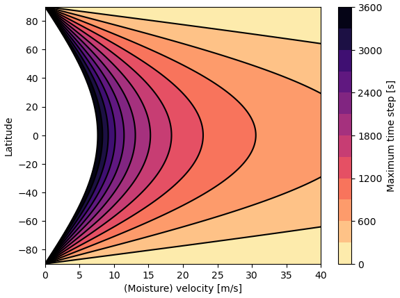
Figure 5 Time step for which the Courant number resolves to unity, based on a grid spacing of 0.25°, as in the ERA5 input data, and a typical range of moisture velocities seen in the example cases.

In principle, the time step should be chosen to be sufficiently small so as to satisfy the Courant–Friedrichs–Lewy (CFL) criterion. However, choosing a very small time step increases the computation time and exacerbates numerical diffusion. So there is an incentive to choose a time step that is sufficiently small for, say, ∼ 95 % of the time and to accept that there may be some extreme circumstances in which the CFL criterion would be violated. In this case, however, we do need to constrain the fluxes for these extremes. To this end, WAM2layers imposes some limits such that the combined moisture fluxes will at most be able to empty the upper or lower grid cell completely. The first limit is such that the meridional and zonal fluxes combined can at most empty the grid cell but cannot create any numerical water gains. The second limit is such that the gross vertical flux can also at most empty the grid cell. These limits are not entirely strict when both horizontal and vertical fluxes are large, which can theoretically lead to numerical tagged moisture gains. However, this is being monitored in the logging and should warrant a reconsideration of the time step.

At the end of each time step, WAM2layers checks against moisture surplus or deficit in any grid cell. Notably, tagged moisture cannot exceed the total moisture in a grid cell. Should there be any imbalance, WAM2layers attempts to redistribute the moisture between the upper and lower layer. If this is not sufficient, tagged moisture is lost from the system internally. In v3, we have added log messages to monitor the ongoing experiment, and the spatial fields are included in the output for later analysis. This provides confidence as long as everything is okay, and it highlights problems early if they arise. Similarly, WAM2layers logs and report transport over the boundary of the domain, which is naturally expected. However, if a research question requires, for instance, an identification of 80 % of the moisture sources, then the boundary transport and where that boundary transport occurred provide information for rerunning the model with a larger domain.

5 Example use cases

Here, we present two example cases to show some of the possibilities of WAM2layers v3. We selected one forward-tracking and one backward-tracking example with a different event duration. The input data and the configuration for these cases are available via the 4TU.ResearchData repository (Benedict and Weijenborg, 2024; Gaasbeek and Van der Ent, 2024), and WAM2layers implements a download utility to automatically retrieve these datasets by their DOI. As such, anyone can easily reproduce these example cases and get started with WAM2layers.

The backward-tracking example case determines the moisture sources of the extreme precipitation event over the Eiffel region in western Europe (Belgium, France, Germany, Luxembourg, and the Netherlands) on 13–14 July 2021. This was a catastrophic event during which extreme precipitation resulted in large floods in the tributaries of the Lower Rhine, such as the Ahr, Erft, and Wupper, and in the tributaries of the Meuse River, such as the Ourthe, Rur, and Geul (Kreienkamp et al., 2021; Mohr et al., 2023). The moisture sources of this event have been previously quantified using different moisture-tracking models, as shown in Insua-Costa et al. (2022) and Staal and Koren (2023), and now by WAM2layers, as presented in Fig. 6. Results show that the evaporative sources of this heavy-precipitation event were mostly located over Germany and France. Moreover, there is a substantial contribution from the Atlantic Ocean and a small contribution from the Mediterranean Sea. The spatial pattern of the sources corresponds to the sources determined by Insua-Costa et al. (2022) and Staal and Koren (2023). Please note that this configuration only considers a limited domain and time span, as it is intended as a lightweight example case. For a full comparison with previous studies, extra simulations are recommended. In this regard, it is worth noting that an intercomparison study of moisture-tracking methods, including WAM2layers, is currently being conducted (Benedict et al., 2024).

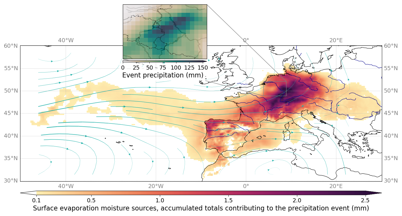
Figure 6 Outcome of the backward-tracking example case “Eiffel”. The figure shows the accumulated tracked moisture sources of the extreme precipitation event of 13–14 July 2021. Total precipitation over the sink region during the event is displayed in the inset. Backward tracking was performed until 1 July. By then, 42 % of moisture was tracked to its source, 3.4 % of was still in the domain's atmosphere, and 54 % was associated with transport across the boundaries of the domain. Streamlines depict the average vertically integrated moisture flow during 1–14 July.

The forward-tracking example case tracks evaporation in the Lake Volta region (Ghana) forward in time for July 1998 to identify the precipitating sinks (Fig. 7). This case was also used in a comparison of moisture-tracking models (Van der Ent et al., 2013), although it is not exactly the same. Input data for the previous study were from the regional climate model MM5 (Knoche and Kunstmann, 2013), the domain was smaller, and the evaporation was tagged during August as well. Nonetheless, we can observe similar moisture sink patterns. These patterns are caused by the southwesterly winds transporting moisture in the lower levels, until the African easterly Jet picks up the tagged moisture and transports it back in a westerly direction towards the Atlantic. Note that the average vertically integrated moisture fluxes alone, as shown by the streamlines in Fig. 7, cannot capture the complicated moisture transport in this system with strong wind shear and, as such, highlight the importance of having two layers in WAM2layers.

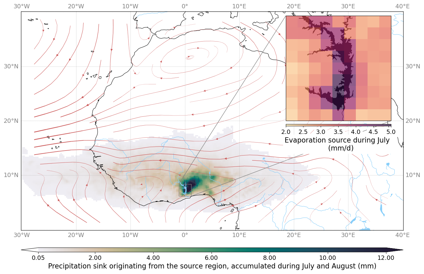
Figure 7 Outcome of the forward-tracking example case “Volta”. The figure shows the tracked moisture sinks of the evaporation from the Lake Volta region during July 1998, although the tracking continued until the end of August 1998. The inset shows the time-averaged evaporation in the source region. A total of 86 % of the total tagged evaporated moisture was attributed to surface precipitation, and 14 % of the tagged moisture was transported across the boundaries of the domain. Of the tagged evaporation, 7.8 % precipitated within the source region. Streamlines depict the average vertically integrated moisture flow during July and August.

6 Best practices in research software development

During the development of WAM2layers v3, we have put a lot of emphasis on the incorporation of research software engineering best practices aimed at making WAM2layers more user-friendly, ensuring that it is easier to maintain, and enabling a more open and transparent scientific process (Barker et al., 2022; Martinez-Ortiz et al., 2023).

One of the key innovations is that WAM2layers has been turned into an installable command-line program. Users no longer need to edit the source code in order to be able to configure their model. Instead, they simply edit a configuration file. This file contains all settings of the model, including the direction of tracking (forward or backward), the internal time step of the model, the interval on which the output data are provided, and the dates for which the tracking should be performed. This makes it easier to share and reproduce experiments. To further enhance reproducibility, WAM2layers creates a dedicated output folder for each experiment, which includes a copy of the configuration file and a log file. Each release of WAM2layers has a corresponding DOI, so users can always refer to the exact version of WAM2layers used for their experiments – here version 3.1 (Van der Ent et al., 2024b).

Importantly, we have added extensive user and developer documentation, which is available at https://wam2layers.readthedocs.io (last access: 14 July 2025). The user documentation includes a quickstart guide, which lets the user run both example cases described in Sect. 5 in a matter of minutes. To this end, we have made WAM2layers available as a Python package on PyPI, such that it can be installed with a single command. Additionally, we have made sample data available at the 4TU.ResearchData repository (Benedict and Weijenborg, 2024; Gaasbeek and Van der Ent, 2024) and added functionality to automatically download these datasets. This could easily be extended to include more reference cases, so we encourage users of WAM2layers to make their cases available in a similar manner. To wrap up the quickstart, WAM2layers includes a quick-analysis module to quickly inspect the input or output of an experiment, but we recommend that users employ more elaborate case-specific code to produce publication-quality figures.

Apart from technical contributions, we have invested in building a welcoming community on GitHub (https://github.com/WAM2layers/WAM2layers/, last access: 14 July 2025). All development happens openly, and we encourage users to engage and contribute through opening issues or pull requests or through the discussion forum where they can ask questions, showcase their results, and share codes. The documentation includes community guidelines and instructions for developing the model as well as an explanation of the collaborative development process. With respect to the developer experience, we have formulated guidelines for code formatting and have set up automated tests to ensure the continuity of the model code. It is verified that results for simple test cases do not change upon making changes to the model code, unless this is expected based on the changes. This strategy is known as “regression testing” (e.g.  Pezze, 2008), and it can provide a lot of confidence for (new) developers.

7 Discussion

Since its inception, the Water Accounting Model (Van der Ent et al., 2010) has evolved from a loose collection of scripts to calculate moisture recycling characteristics into a widely used atmospheric-moisture-tracking software with a broad range of applications (Fig. 2). This paper documents WAM2layers v3 (Van der Ent et al., 2024a), which forms a solid basis for future experiments and further development. Here, we discuss some key strengths as well as aspects where we think the model could still be improved.

7.1 Important simplifications

In WAM2layers, the evolution of (tagged) moisture is completely governed by precipitation, evaporation, and redistribution through advection, vertical mixing, and (artificially) numerical diffusion. Horizontal mixing, microphysics, and other subgrid processes are omitted. These simplifications, partly born of necessity, introduce inaccuracies that users of WAM2layers should beware of. Below, we discuss these simplifications in more detail and how future work may test the importance of these simplifications and potentially improve on them.

Historically, WAM2layers has always operated on the same grid as the input data, i.e. reanalysis and climate model output that is typically retrieved at an equirectangular latitude–longitude grid. As shown in Sect. 4, this limits its applicability over polar areas. While alternatives exist, assumptions about the current grid structure are deeply woven into the implementation; thus, changing this structure is not trivial, especially as we foster continuity of the codebase to keep existing users on board and avoid alienation. Nonetheless, WAM2layers v3 includes substantial efforts to improve the code structure, isolating the solver and related numerical aspects from other parts of the code that deal with things like I/O and orchestration. This enables experimentation with different solvers, which could eventually enable a different core design. For research questions that focus on moisture transport over polar areas (but not globally), a more feasible workaround could be to remap the input data to another equirectangular grid that is optimized for polar areas. This would keep the existing assumptions intact, although it would still require various code changes that are beyond the scope of this paper.

The donor cell scheme employed in WAM2layers (i.e. the “upstream” or “Godunov” scheme) has some favourable properties: it is simple, intuitive, conservative, and numerically stable. Above all, it does not permit overshoot or undershoot, which is a highly suitable property for a moisture-tracking model considering the absolute minimum of 0 (tagged) moisture. On the downside, this scheme is known to be numerically diffusive (Hourdin and Armengaud, 1999), and this artificial diffusion may even exceed the true physical diffusion, which is undesirable (Cushman-Roisin and Beckers, 2011). It limits WAM2layers' usability at high latitudes and may lead to an overestimation of far away sources. Ideally, one would want to suppress or eliminate numerical diffusion altogether (or at least be able to quantify it). One option could be to explore the use of alternative solvers, such as flux limiters (Hourdin and Armengaud, 1999; Cushman-Roisin and Beckers, 2011) or MPDATA (Smolarkiewicz and Margolin, 1998). WAM2layers v3 isolates the numerical solver such that is becomes easier to experiment with such alternatives. However, we emphasize that any changes in this regard should be carefully evaluated to ensure that their benefits outweigh the existing advantages.

WAM2layers uses water vapour as a proxy for total water, and it does not represent microphysical processes associated with phase changes or the transport of ice and liquid water. This is a common limitation in offline moisture-tracking models (e.g.  Cheng and Lu, 2023; Dey and Döös, 2020; Dirmeyer and Brubaker, 1999; Holgate et al., 2020; Keune et al., 2022; Sodemann et al., 2008; Tuinenburg and Staal, 2020). As discussed in Sect. 3, we can sometimes partly correct the states and horizontal fluxes for the presence of ice and liquid water via the application of Eq. (19). However, condensation and re-evaporation may be most relevant in the vicinity of precipitation, in which case they could bring about a strong vertical exchange of (tagged) moisture, e.g. condensating in the upper layer and re-evaporating in the lower layer. This is one of the reasons why it is important to realize that the vertical transport term, which is calculated as a closure term in WAM2layers, effectively acts as a generic redistribution term, incorporating the effects of unresolved processes, such as microphysics and (turbulent) diffusion, and even compensating for discontinuities in the input data or errors in the horizontal fluxes.

Finally, a note on the reduction to two layers. Van der Ent et al. (2013) found that a two-layer model was both necessary and sufficient to represent large-scale atmospheric moisture transport. The two-layer model simplifies the computation of the vertical moisture flux and the partitioning of precipitation between the layers of the model. However, it also leads to a two-step procedure in which all 3D fields first need to be aggregated onto the new grid. Generalizing to N layers (where N corresponds to the number of levels in the input data) could potentially simplify the code. However, it remains to be seen whether this would actually improve the results, as a correct representation of all vertical exchange processes would remain challenging and should be thoroughly tested.

7.2 A note on performance

WAM2layers v3 is written in Python. This programming language is very popular among (atmospheric) scientists, which makes it easy to use. Moreover, Python's simple syntax makes it easy to understand the models internal workings, which we deem key from a transparency point of view. However, Python has somewhat of a poor reputation when it comes to computational performance. Evidently, the use of numerical computing libraries such as NumPy alleviates this to a certain extent (Harris et al., 2020; Langtangen and Cai, 2008). Further performance gains could potentially be achieved by using dedicated libraries for stencil computations or by porting some of the performance-critical code to more performant languages. A potential downside of using experimental third-party libraries or mixing languages is that it puts a bigger constraint on the maintainability of the software. Therefore, treading this path remains a balancing act, and we tend to favour usability and code transparency over performance.

7.3 Future developments

Software development is planned to continue after the WAM2layers release associated with this paper (version 3.1.0 at the time of writing). Future developments notably aim to bring back some old features that have not yet been ported to version 3, such calculations for moisture recycling within a single grid cell for all grid cells of the domain at once (e.g.  Van der Ent and Savenije, 2011; De Hertog et al., 2024), time tracking (e.g.  Van der Ent et al., 2014; Van der Ent and Tuinenburg, 2017), distance tracking (e.g.  Guo et al., 2019, 2020), and advanced spline interpolation of the humidity profile in the case of limited vertical information (Benedict et al., 2020). We are planning to reincorporate these features in a backwards-compatible manner. Similarly, we would also like to port preprocessing codes for other reanalyses datasets (e.g.  Keys et al., 2024; Li et al., 2022) as well as climate model output with which WAM2layers has been used in the past (e.g.  Bosmans et al., 2020; De Hertog et al., 2024; Findell et al., 2019; Guo et al., 2020) to future model releases.

In developing WAM2layers v3, we have made substantial efforts to generalize the derivation presented here and to isolate the implementation of the numerical scheme in the code. We believe that this work, together with the changes made for WAM2layers v3, forms a good basis for modelling exercises such as implementing alternative solvers or further increasing the performance.

Concurrently to writing this article, we are co-organizing a coordinated moisture-tracking intercomparison study (Benedict et al., 2024) to gain an understanding of the uncertainties in different tracking methods. We expect that these community activities will help to (1) shed a better light on the strengths and weaknesses of WAM2layers and other models and (2) gain confidence in moisture tracking results in general.

8 Conclusions

To conclude, this paper fills an important gap in the documentation of a widely used atmospheric-moisture-tracking model. We have provided an updated description of the model that facilitates comparison with other models and literature and have pointed out some important assumptions, which facilitates the interpretation of past and future results obtained with WAM2layers.

This paper and the associated v3 release mark a new milestone in the evolution of WAM2layers. While the core tracking principle and assumptions remain unchanged, the code is now much more efficient and modular, making it ready for future developments. We have pointed out several directions for future work, including a more thorough investigation of the numerical aspects and opportunities for improved model validation in collaboration with the moisture-tracking community.

With the incorporation of various best practices, as outlined in the practical guide to software management plans (Martinez-Ortiz et al., 2023), and engagement with the wider community, we have made important steps to carry out FAIR (Barker et al., 2022) and open, collaborative research software development, and we are committed to improving this further into the future. We hope that this approach will inspire others to follow suit, as we believe that transparency and collaboration are crucial for the credibility of prosperity of the scientific field.