A time-dependent three-dimensional dayside magnetopause model based on quasi-elastodynamic theory

The interaction between the solar wind and Earth's magnetosphere is a critical area of research in space weather and space physics. Accurate determination of the magnetopause position is essential for understanding magnetospheric dynamics. While numerous magnetopause models have been developed over past decades, most are time-independent, limiting their ability to elucidate the dynamic movement of the magnetopause under varying solar wind conditions. This study introduces the first time-dependent three-dimensional magnetopause model based on quasi-elastodynamic theory, named the POS (Position–Oscillation–Surface wave) model. Unlike existing time-independent models, the POS model physically reflects the dynamic responses of magnetopause position and shape to time-varying solar wind conditions. The predictive accuracy of the POS model was evaluated using 38 887 observed magnetopause-crossing events. The model achieved a root-mean-square error of 0.774 Earth radii (R_E, representing a 17.9 % improvement over five widely used magnetopause models. Notably, the POS model demonstrated superior accuracy under highly disturbed solar wind conditions (22.1 % better) and in higher-latitude regions (27.0 % better) and flank regions (33.3 % better) of the magnetopause. The POS model's remarkable accuracy, concise formulation, and fast computational speed enhance our ability to predict magnetopause position and shape in real time. This advancement is significant for understanding the physical mechanisms of space weather phenomena and improving the accuracy of space weather forecasts. Furthermore, this model may provide new insights and methodologies for constructing magnetopause models for other planets.

1 Introduction

The magnetopause, the boundary between the interplanetary magnetic field (IMF) and Earth's magnetic field, plays a crucial role in space weather forecasting and in understanding solar wind–magnetosphere coupling mechanisms (Willis, 1971; Song et al., 1996; Russell, 2003). It acts as a protective shield against hazardous energetic particles while simultaneously serving as the primary interaction region for solar wind–magnetosphere coupling. The magnetopause exhibits considerable dynamic behaviour due to continuous solar wind variations and various instabilities – even under steady solar wind conditions (Anderson et al., 1968; Song et al., 1988; Eastwood et al., 2015). These dynamics can lead to radiation-belt particle loss, field-aligned current intensification, ultra-low-frequency wave generation, and solar wind energy conversion, which affect the radiation belts, polar regions, and ionosphere (Haerendel, 1990; Mann et al., 2012; Plaschke, 2016; Mottez, 2016; Archer et al., 2019). Consequently, comprehending the interactions between the solar wind and the magnetopause is vital for advancing magnetospheric dynamics and improving space weather prediction capabilities (Feng, 2020; Zong et al., 2020).

Numerous magnetopause models have been established over the past few decades, generally categorized as physical (or principal) models (Ferraro, 1952; Beard, 1960; Spreiter et al., 1966) and empirical models (Fairfield, 1971; Tsyganenko, 1989; Shue et al., 1998; Lin et al., 2010). Physical models are primarily based on the classic Chapman–Ferraro theory proposed in the 1930s (Chapman and Ferraro, 1930), which states that the magnetopause's equilibrium position is determined by the pressure balance between solar wind dynamic pressure (P_dyn) and magnetospheric magnetic pressure (P_b). Since the 1960s, the launch of numerous satellites has provided us with a large number of samples of magnetopause-crossing events (MCEs), thereby creating the possibility for the establishment of empirical models (Fairfield, 1971; Sibeck, 1991; Petrinec and Russell, 1996; Shue et al., 1998; Lin et al., 2010). Many empirical models rely on two key parameters, P_dyn and IMF B_z, and some models use the Earth's dipole tilt angle (Φ) to calibrate the higher-latitude zone. Besides, some empirical models proposed in the 1980s combine physical processes of solar wind–magnetosphere interactions with satellite observation fitting and involve the impact of the magnetospheric current system (Tsyganenko, 1989; Tsyganenko and Stern, 1996). Regardless of the assumptions on which these models are based, all these models have contributed to our understanding of magnetopause movement and its response to solar wind conditions. In particular, many of them have been widely used in the prediction of the magnetopause due to their simple form and high prediction accuracies.

However, it should be stated that these models primarily describe the average steady-state characteristics of the magnetosphere. To accurately describe the dynamic coupling process of solar wind–magnetosphere interaction, it is essential to incorporate time-partial derivatives into dynamic equations (Smit, 1968; Petrinec, 2001; Borovsky and Alejandro Valdivia, 2018). This approach, however, complicates the solution of model equations, often necessitating numerical simulations such as magnetohydrodynamic (MHD) simulations (Powell et al., 1999; Raeder et al., 2001; Lyon et al., 2004; Tóth et al., 2005; Merkin and Lyon, 2010), particle-in-cell (PIC) simulations (Moritaka et al., 2012; Ashida et al., 2014; Walker et al., 2019), and hybrid simulations (Gargaté et al., 2008; Omelchenko et al., 2021; Ala-Lahti et al., 2022). Numerical simulations are widely used in exploring solar wind–magnetosphere coupling and can accurately reveal the position of the magnetopause changing with the time-varying solar wind conditions. Collado-Vega et al. (2023) compared the magnetopause predictions obtained from different MHD models, showing the discrepancies in the standoff position. Their analysis also specifically addressed the impact of extreme solar wind conditions, which are known to cause space weather hazards, on the magnetopause. However, the introduction of time-partial derivatives makes equations very difficult to solve. Additionally, many prominent numerical simulation models may not properly include all magnetospheric current systems (e.g. the ring current or the magnetospheric–ionospheric currents); therefore, this omission may result in systematic errors in the magnetopause prediction (Samsonov et al., 2016). Moreover, numerical models are solved on supercomputers, consuming a significant amount of computing resources and time, rendering them impractical for real-time space weather forecasting (Raeder et al., 2001; Lyon et al., 2004; Tóth et al., 2005; Feng, 2020). This limitation highlights the need for more efficient yet accurate magnetopause models that can capture the dynamic nature of the magnetopause while remaining computationally feasible for real-time applications. Such models would significantly enhance our ability to predict and understand space weather phenomena, bridging the gap between theoretical understanding and practical forecasting capabilities.

Apart from numerical simulations, very few time-dependent magnetopause models have been historically developed (Smit, 1968; Børve et al., 2011; Freeman et al., 1995; Sato et al., 2022). Figure 1 illustrates the fundamental difference between time-independent and time-dependent models. In time-independent models, the magnetopause position is directly correlated with instantaneous solar wind conditions. For example, a step-like increase in solar wind dynamic pressure (such as a shock) corresponds to an immediate step-like compression of the magnetopause (Fig. 1a). However, this simplification fails to capture the real dynamics of the magnetopause. In reality, the magnetopause undergoes a more complex process of compression and recovery, exhibiting oscillatory characteristics in response to abrupt changes in solar wind conditions, as shown in Fig. 1b (Freeman and Farrugia, 1998; Hu et al., 2005; Desai et al., 2021). Time-dependent models aim to capture these dynamic processes, providing a more accurate representation of magnetopause behaviour. To describe these dynamic responses, it is necessary to incorporate time-partial derivatives into the governing equations. However, this inclusion significantly complicates the solution process. Consequently, existing time-dependent models are predominantly one-dimensional and remain in a preliminary stage of development.

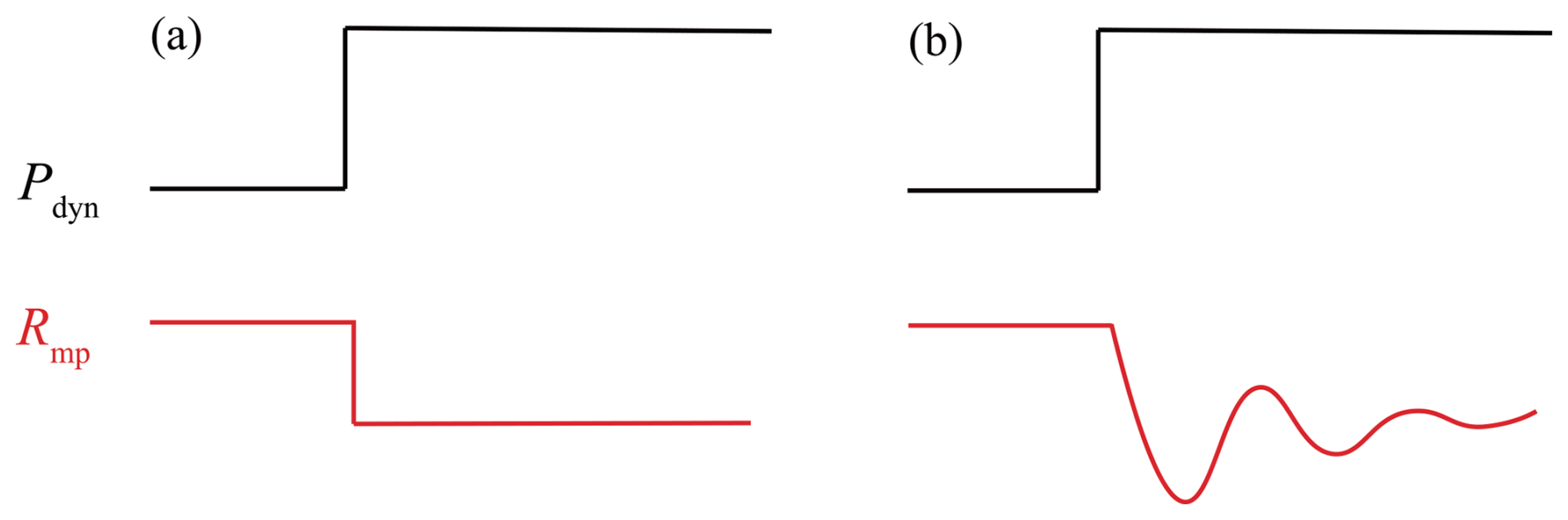
Figure 1 The schematic diagram of time-independent (a) and time-dependent (b) magnetopause models.

Smit (1968) conceptualized the magnetopause as a rigid surface and attempted to explain its motion from the perspective of periodic vibration; Freeman et al. (1995) investigated the influence of inertial and damping effects on the magnetosphere, employing magnetohydrodynamics to analyse the magnetopause motion; and Børve et al. (2011) set up a non-adjustable model to analyse the oscillation period of the magnetopause. By investigating the movement of the subsolar point in response to time-varying solar wind conditions, these models are primarily constructed to elucidate specific physical phenomena linked to solar wind–magnetosphere interaction, yet they lack the capability to provide a real-time depiction of the three-dimensional magnetopause position and shape.

Hence, the challenge of constructing time-dependent models lies in balancing the need for accurate dynamic representation with computational feasibility. Although time-dependent models offer a more realistic depiction of magnetopause behaviour, their complexity has limited their development and application, particularly in three-dimensional space. This highlights the necessity for new strategies that can capture time-dependent dynamics while ensuring practical utility for computation, especially for real-time space weather forecasting and related magnetospheric research. Previously, our work revealed the quasi-elastodynamic processes involved in the interaction between the solar wind and the magnetosphere (Gu et al., 2023). It suggests that the dynamic behaviour of each point on the magnetopause can be viewed as an equilibrium position (P), as radial global oscillations around the equilibrium position (O), and as a surface-wave-like structure around the flank regions (S). This work offers a practical framework for developing a time-dependent three-dimensional magnetopause model.

However, our previous work primarily focused on elucidating the quasi-elastic process, with less emphasis on the outcomes of model predictions (Gu et al., 2023). Key factors influencing magnetopause dynamics, such as the IMF B_z and Earth's dipole tilt angle (Φ), were not incorporated. Additionally, the adjustable parameters in the equations were simply chosen and lacked thorough calibrations. Moreover, our prior work and most published magnetopause models (Petrinec and Russell, 1996; Shue et al., 1998; Gu et al., 2023) relied on a relatively limited dataset of low-latitude satellite observations, leading to constraints in accurately representing the higher-latitude and flank regions of the magnetopause. To address these limitations and overcome the inherent shortcomings of time-independent models, particularly their inability to reflect the dynamic responses of the magnetopause position and shape to time-varying solar wind conditions, we propose a time-dependent three-dimensional magnetopause model. This model, which has been tested with the largest dataset of MCEs to date (38 887 events), demonstrates remarkable prediction accuracy compared to those of five widely used magnetopause models. Besides, it offers unparalleled real-time computation speed and a concise form relative to numerical simulations. We have named this model the position–oscillation–surface wave (POS) model.

2 Datasets and other magnetopause models for comparison

The THEMIS (Time History of Events and Macroscale Interactions during Substorms) mission (Angelopoulos, 2008), which consists of five spacecraft launched into similar elliptical, near-equatorial orbits in 2007, has significantly enhanced our ability to observe the magnetosphere. The mission provides high-resolution (∼ 3 s) magnetic field measurements through the THEMIS/Fluxgate Magnetometer (FGM) (Auster et al., 2008) and plasma data from the THEMIS/Electrostatic Analyser (EA) (McFadden et al., 2008). The CLUSTER II mission (Escoubet et al., 2001), involving four identical spacecraft launched in 2000, also offers high-resolution (∼ 4 s) magnetic field measurements using the CLUSTER/Fluxgate Magnetometer (FGM) (Balogh et al., 1997), particle data, and moments from the CLUSTER Ion Spectrometry-Hot Ion Analyser (CIS–HIA) (Rème et al., 1997).

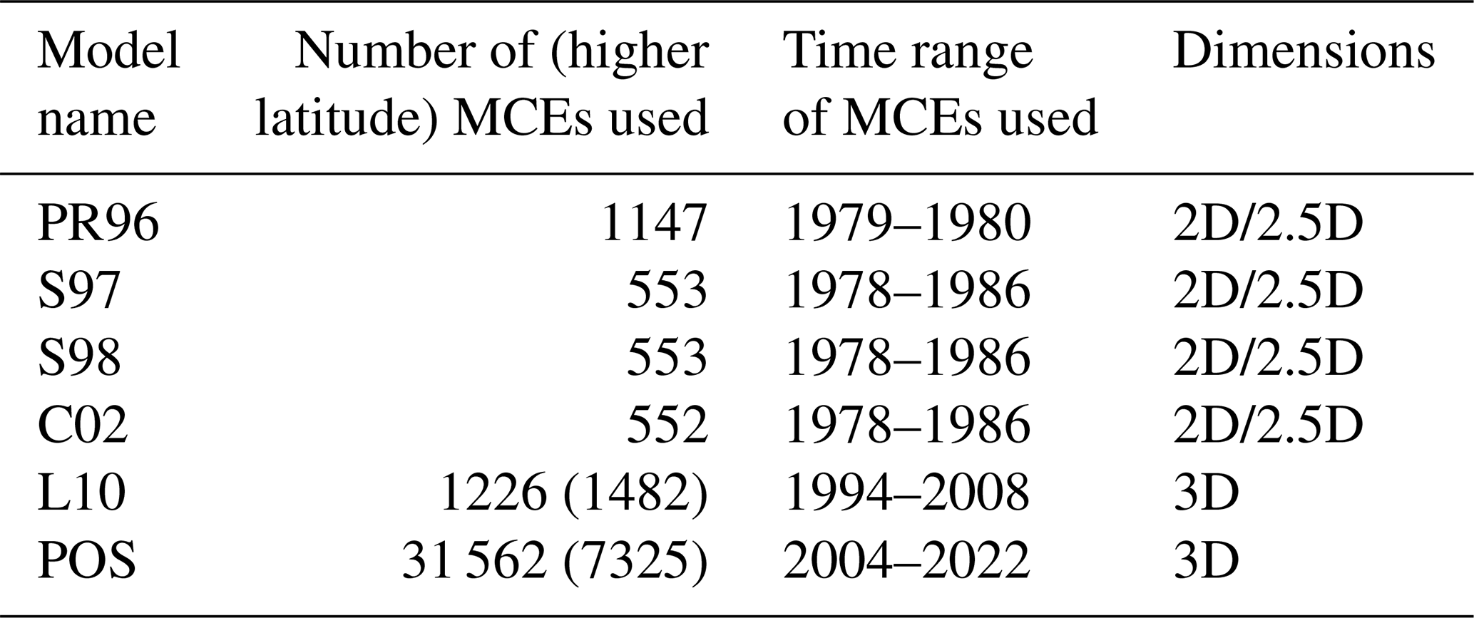
The WIND spacecraft, launched into orbit around Earth in 1994 and relocated to the Lagrange L1 point after 2004, provides continuous, high-quality in situ solar wind observations. This study utilizes high-resolution (∼ 3 s) plasma data from the WIND/3D Plasma Analyzer (3DP) (Lin et al., 1995) and magnetic field data from the Magnetic Fields Investigation (MFI) (Lepping et al., 1995) for upstream solar wind observations. For this study, we have compiled a dataset consisting of 51 590 THEMIS MCEs and 38 321 CLUSTER MCEs. After excluding redundant crossings (i.e. those occurring simultaneously on the same satellite), invalid data (i.e. crossings without valid upstream solar wind observations), and nightside MCEs (where X_GSM<0 R_E), 38 018 THEMIS MCEs and 869 CLUSTER MCEs (see Fig. 2) are selected for this study. The time shift (δt) from WIND and the satellite MCE is determined by comparing the time of each crossing (t₁) with the probable arrival time of the corresponding solar wind observation from WIND (t₀+δt), satisfying (t₀+δt)− t₁<300 s. The 300 s threshold is set as the potential error window for the time shift from L1 to the magnetopause. δt, calculated as (L1−r)$/$ 〈v_x〉, L1 (L1 = 235 R_E), is the distance from the Earth to the L1 point, r denotes the radial position of the magnetopause, and 〈v_x〉 is the 1 h sliding average of the solar wind velocity in the x component (Chao et al., 2002). A summary of these events is provided in Table 1. The distribution of matched solar wind conditions for MCEs is shown in Fig. 3. All data are available in the CDAWeb database (http://cdaweb.gsfc.nasa.gov/, last access: 24 July 2024), and the time resolutions of both the magnetic field and plasma data used in the study are interpolated to a 3 s resolution, set in GSM coordinates.

Table 1 Summary of 89 911 satellite MCEs and datasets used in this paper.

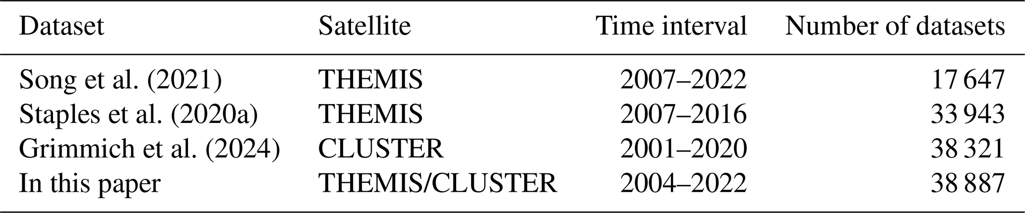
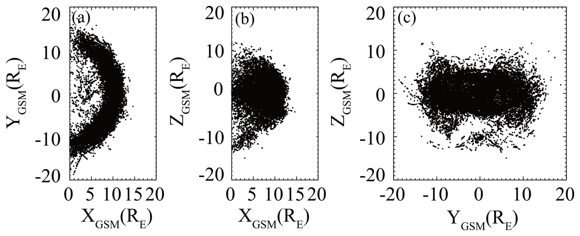
Figure 2 Projections of 38 887 MCEs in the GSM coordinate (a) X–Y plane, (b) X–Z plane, and (c) Y–Z plane.

In previous research on time-independent magnetopause models, the physical models (Ferraro, 1952; Beard, 1960; Spreiter et al., 1966), although theoretically grounded, usually oversimplify intricate solar wind–magnetosphere interactions to facilitate calculations, usually without demonstrating apparent higher prediction accuracies compared to widely used empirical models (Petrinec and Russell, 1996; Shue et al., 1997; Shue et al., 1998; Chao et al., 2002; Lin et al., 2010). Hence, this article concentrates on comparing several notable time-independent empirical models renowned for their superior prediction accuracies (Petrinec and Russell, 1996; Shue et al., 1997; Shue et al., 1998; Chao et al., 2002; Lin et al., 2010).

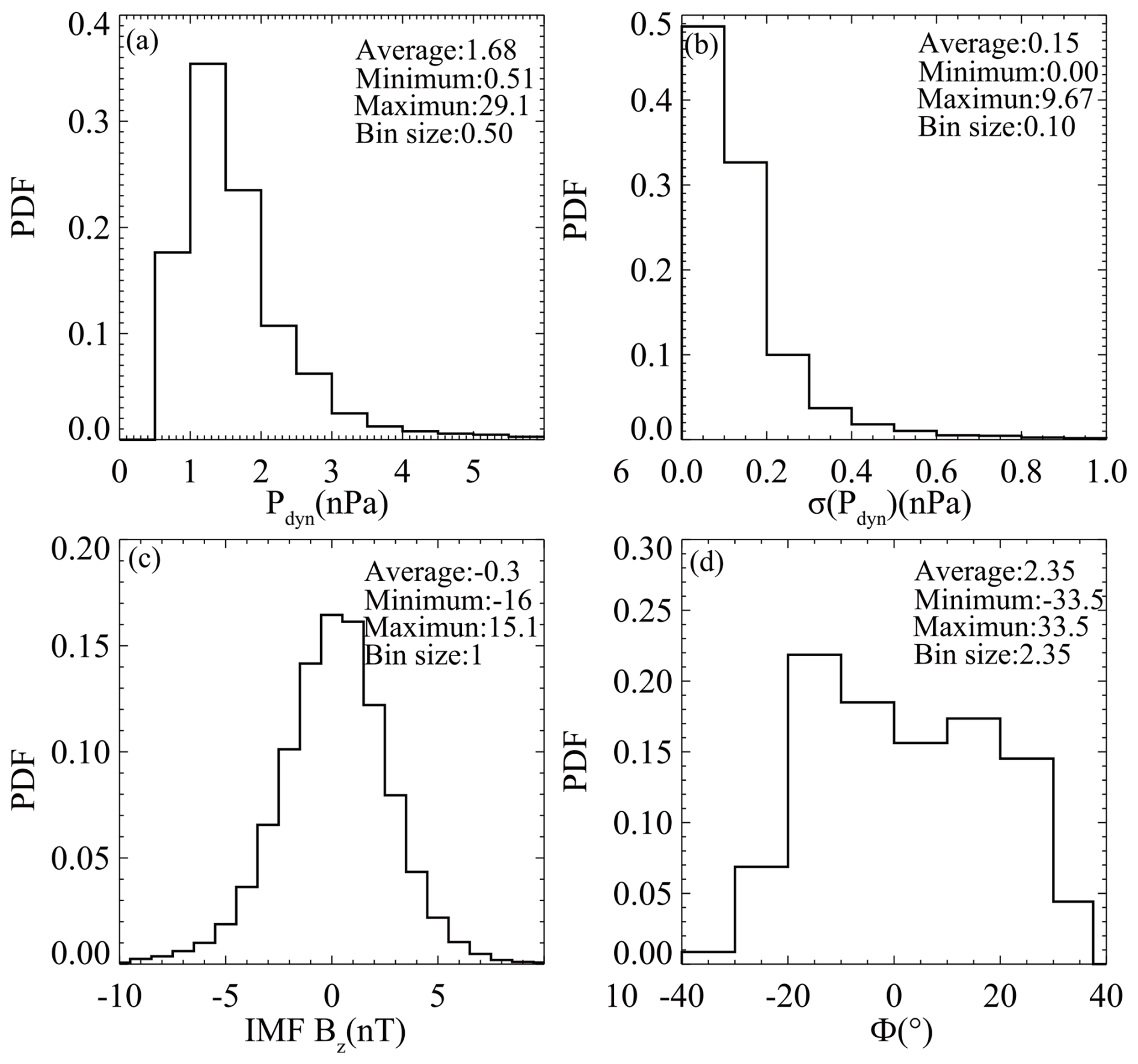
Figure 3 Probability density function of upstream solar wind observations in terms of (a) the solar wind dynamic pressure (P_dyn), (b) the standard deviation of dynamic pressure (P_dyn), (c) the interplanetary magnetic field B_z component (IMF B_z), and (d) the dipole tilt angle (Φ).

Empirical models are typically constructed using satellite observations of MCEs. While these models vary in their use of satellite datasets, parameters considered, coordinate systems employed, and functions applied, most are parameterized using the dynamic pressure (P_dyn) and the interplanetary magnetic field B_z component (IMF B_z). For example, Petrinec and Russell (1996) (hereafter PR96) employed an ellipsoidal function to construct a magnetopause model, while Shue et al. (1997) (hereafter S97) developed a flexible function incorporating two variables: the subsolar magnetopause position (R₀) and the tail flaring angle (α). This function has gained widespread use as a foundational approach to describing magnetopause shape. For instance, Shue et al. (1998) (hereafter S98) accounted for the saturation effect of the IMF B_z on R₀, and Chao et al. (2002) (hereafter C02) extended their model for application under normal and extreme solar wind conditions.

Nevertheless, these models primarily rely on low-latitude satellite observations and may not adequately capture the distinctive characteristics of the magnetopause in the higher-latitude region. Besides, they are constructed with the P_dyn and the IMF B_z, while it is found that the dipole tilt angle Φ is of great significance when modelling the magnetopause, especially in the higher-latitude region. Formisano et al. (1979) constructed an average magnetopause size and shape for two dipole tilt angle values (Φ). Boardsen et al. (2000) developed a higher-latitude magnetopause model parameterized not only by the P_dyn and the IMF B_z but also by the dipole tilt angle (Φ), recognizing its significant influence on the shape of the higher-latitude region of the magnetopause. While this model is specifically designed for higher-latitude regions, it is not as effective in accurately calculating the magnetopause at low latitudes compared to other models due to inherent limitations.

Table 2 Summary of five widely used magnetopause models and the POS model.

The above models are generally developed under the assumption of axial symmetry, while the actual magnetopause shape is asymmetrical in both the Y and Z directions, so they are essentially 2D or 2.5D models. To describe the 3D structure of the magnetopause, Lin et al. (2010) (hereafter L10) developed a three-dimensional magnetopause model parameterized by the P_dyn, the thermal pressure (P_t), the IMF B_z, and the Φ. The coordinate systems employed in these empirical models are typically comprised of aberrated coordinates, which account for Earth's orbital motion (Petrinec and Russell, 1996; Shue et al., 1997; Shue et al., 1998; Chao et al., 2002), or corrected coordinates which compensate for both Earth's orbital motion and deviations in solar wind velocity from the Sun–Earth line (Boardsen et al., 2000; Lin et al., 2010). A summary of the five widely used magnetopause models is presented in Table 2.

3 The POS model

In our previous work (Gu et al., 2023), we modelled the compression–recovery process of the magnetopause as a quasi-elastodynamic phenomenon. In this framework, the dynamic pressure, $P_{\mathrm{dyn}}=n_{\mathrm{sw}}{m}_{\mathrm{p}}{v}_x^{\mathrm{2}}$, serves as the driving force on the system, where n_sw, m_p, and v_x are the number density, proton mass, and x component of the solar wind velocity in GSM coordinates, respectively. The system's restoring force is described by $P_{\mathrm{b}}=B^{\mathrm{2}}/\mathrm{2}{\mathit{\mu }}_{\mathrm{0}}$, where B is the total magnetic field at the magnetopause and μ₀ is the vacuum permeability. After accounting for damping and non-ideal effects, P_damp, and excluding the complex coupling interactions, the momentum equation for the magnetosheath in a unit cylinder can be represented by Eq. (1).

$$\begin{array}{}\text{(1)}& M_{\mathrm{msh}}{a}_{\mathrm{msh}}=P_{\mathrm{b}}-P_{\mathrm{dyn}}-P_{\mathrm{damp}}\end{array}$$

Given that the derivation process of the foundational formula is the same as our previous work and that this paper is focused on model predictions rather than physical processes, we will refrain from reiterating it here. The relationship depicting the temporal evolution of the magnetopause position (r) is introduced in Eq. (2):

$$\begin{array}{}\text{(2)}& \begin{array}{rl}{n}_{\mathrm{sw}}{m}_{\mathrm{p}}r\ddot{r}& ={\displaystyle \frac{\left(\mathit{\lambda }{\mathit{B}}_{\mathrm{d}}\right(r,\mathit{\theta },\mathit{\phi })+{\mathit{B}}_c(r,\mathit{\theta },\mathit{\phi }){)}^{\mathrm{2}}}{\mathrm{2}{\mathit{\mu }}_{\mathrm{0}}}}\\ & -n_{\mathrm{sw}}{m}_{\mathrm{p}}{\mathit{v}}_x^{\mathrm{2}}{\cos }^{\mathrm{2}}\mathit{\alpha }-k{\mathrm{\Sigma }}_{\mathrm{p}}{\mathit{B}}_{\mathrm{p}}^{\mathrm{2}}\dot{r}-\mathit{\eta }\dot{r}/r,\end{array}\end{array}$$

where r, θ, and ϕ represent the corresponding spherical coordinates. The variable r is the radial distance; θ is the latitude angle in the range [−90°, 90°]; and φ is the longitude angle, adjusted to the range [−180°, 180°] with 0° oriented towards the Sun for simplicity – all the vectors have been projected to the normal direction of the magnetopause (Gu et al., 2023). This simplified equation enables us to capture the fundamental dynamics of the magnetopause's response to solar wind fluctuations while ensuring computational efficiency. The first term on the right side of Eq. (2) signifies the restoring force P_b. Here, B_d denotes the Earth's dipole field, λ is the magnetospheric compressibility coefficient, and B_c accounts for contributions from various magnetospheric currents. The second term on the right side represents the driving force P_dyn, where α denotes the angle between the x direction and the normal direction of the magnetopause. The third term on the right side of Eq. (2) characterizes a position-dependent dragging effect estimated from the ionosphere. The fourth term illustrates a global non-ideal viscous effect. B_p is the estimated ionospheric magnetic field in the polar region, Σp stands for the equivalent Pederson conductivity, k serves as a position-dependent mapping factor, and η represents the viscous coefficient. The final two terms contribute to the damping and non-ideal effects of the system, denoted as P_damp. Equation (2) provides a foundation for developing a time-dependent magnetopause model that can reflect the system's dynamic behaviour more accurately compared to conventional time-independent models. We will introduce the key parameters in detail in the following sections. All the parameters are in SI units.

In this study, we incorporate the impact of IMF B_z and Φ in the magnetospheric magnetic pressure. To determine the equation's final fitting coefficients, we conducted 1000 independent iterations, each involving a random selection of 5000 MCEs from our dataset of 38 887 MCEs.

3.1 The magnetospheric compressibility coefficient (λ)

The magnetospheric compressibility coefficient, λ, measures the magnetosphere's response to solar wind pressure, specifically the ratio of the magnetospheric magnetic field to the pure dipolar magnetic field (Spreiter et al., 1966; Schield, 1969). This coefficient is one of the most critical parameters directly affecting the position of the magnetopause. Typically, λ has a value of 2.44 at the subsolar point, but it changes as the magnetopause shifts and varies with latitude and longitude, suggesting a more complex formulation (Shue et al., 2011; Chen et al., 2023). Mead and Beard (1964) used a self-consistent method and discovered an inward-concave structure at the higher-latitude magnetopause, which is influenced by the inclination angle of Earth's dipole. Their work also determined the surface shape of the magnetopause when the solar wind flow is perpendicular to the dipole axis (Φ=0°), providing an expression for λ as a function of the angles θ and φ.

Several models (Formisano et al., 1979; Boardsen et al., 2000; Lin et al., 2010) have been developed to investigate the influence of Φ (the angle between Earth's magnetic axis and the solar wind direction) on the magnetopause's position and shape, offering valuable insights into the magnetosphere's three-dimensional structure. These models predict an asymmetrical response of the magnetosphere to variations in Φ. Boardsen et al. (2000) quantified the effects of Φ on the higher-latitude region of the magnetopause using MCE data from the Northern Hemisphere. Their work revealed how the dipole tilt angle influences the magnetopause structure in polar regions, which are particularly sensitive to changes in the orientation of Earth's magnetic field relative to the solar wind. Lin et al. (2010) further demonstrated that an increase in Φ causes a slight shift in the centres of the magnetopause cross-sections, moving them towards the negative Z direction in the subsolar region and towards the positive Z direction in the tail region. According to Olson (1969), who provided a detailed representation of λ for various tilt angles (Φ = 0, 10, 20, 30°) on a 15°×15° grid of θ and φ values, the dipole tilt angle significantly alters the fundamental behaviour of λ, with varying effects on θ and φ. This influence is more pronounced in higher-latitude regions (θ>30°). Building on previous work by Gu et al. (2023), in which $\mathit{\lambda }=\mathrm{2.44}-\mathrm{0.4}{\mathit{\theta }}^{\mathrm{2}}+{\mathit{\phi }}^{\mathrm{2}}$, we incorporate the effect of Φ on different positions of the magnetopause λ(θ,φ) and derive a more precise expression for λ, specifically tailored to our model, as presented in Eq. (3):

$$\begin{array}{}\text{(3)}& \begin{array}{rl}A& =\tanh \left[\mathrm{5.568}(\left|\mathit{\theta }\right|-\mathrm{0.5325})\right]+\mathrm{1.0}\\ & \mathit{\lambda }(\mathit{\theta },\mathit{\phi },\mathrm{\Phi })=\mathrm{2.44}-(\mathrm{0.4}+\mathrm{0.3}A)(\mathit{\theta }+\mathrm{0.2}A\mathrm{\Phi }{)}^{\mathrm{2}}\\ & +(\mathrm{1.0}-\mathrm{0.5}A\left|\mathrm{\Phi }\right|){\mathit{\phi }}^{\mathrm{2}}.\end{array}\end{array}$$

3.2 Contributions from various magnetospheric currents (B_c)

Previous studies on the impact of magnetospheric currents on the position of the magnetopause led to the development of a static magnetopause current model, where the magnetic fields of the magnetopause surface currents and tail currents were fitted using polynomials to reveal the relationship between variations in the magnetospheric magnetic field and changes in magnetopause position, e.g. $B_{\mathrm{surf}}(r,\mathit{\theta },\mathit{\phi })$ and $B_{\mathrm{tail}}(r,\mathit{\theta },\mathit{\phi })$ (Choe and Beard, 1974a, b; Matsuoka et al., 1995). In our earlier study (Gu et al., 2023), the magnetic field of the current system, denoted as B_c0 (r), did not account for variations in θ and ϕ. This limitation is addressed in the present study. The fundamental form of B_c0 $(r,\mathit{\theta },\mathit{\varphi })$, incorporating these angular dependencies, is introduced in Eq. (4). The current system exhibits asymmetrical effects consistent with other models such as T96 and T01 (Tsyganenko, 2001; Tsyganenko and Stern, 1996). These models also incorporate dawn–dusk asymmetry in the magnetospheric current, reflecting the influence of these angular dependencies.

$$\begin{array}{}\text{(4)}& \begin{array}{rl}{\mathit{B}}_{\mathrm{c}\mathrm{0}}(r,\mathit{\theta },\mathit{\phi })& =[-\mathrm{401}\mathrm{904}/{\left({\displaystyle \frac{r}{R_{\mathrm{E}}}}\right)}^{\mathrm{4}}+\mathrm{65}\mathrm{489}/{\left({\displaystyle \frac{r}{R_{\mathrm{E}}}}\right)}^{\mathrm{3}}\\ & +\mathrm{1500}/{\left({\displaystyle \frac{r}{R_{\mathrm{E}}}}\right)}^{\mathrm{2}}-\mathrm{40}\left]\right[\mathrm{1}+\mathrm{0.4}\sin \left(\mathrm{2}\mathit{\theta }{)}^{\mathrm{2}}\right]\\ & [\mathrm{1.0}-\mathrm{0.1}\sin (\mathit{\phi }\left)\right]\times {\mathrm{10}}^{-\mathrm{9}}\end{array}\end{array}$$

In our previous work, B_c(r) was defined as a piecewise function of P_dyn, which could yield discontinuous and non-physical results at the transition points (Gu et al., 2023). To address this limitation, we now consider the impact of P_dyn in a continuous form, eliminating the piecewise dependence. Furthermore, the impact of the IMF B_z on the magnetopause position is directionally dependent, with a southward IMF triggering dayside magnetic reconnection, an essential process already incorporated in most existing models (Aubry et al., 1970; Dungey, 1961; Fairfield, 1971). To quantify this effect, we adopt a hyperbolic tangent function, similar to that used in Shue et al. (1998). Finally, by considering the combined effects of both IMF B_z and P_dyn, B_c is expressed as follows in Eq. (5):

$$\begin{array}{}\text{(5)}& \begin{array}{rl}{\mathit{B}}_{\mathrm{c}}& ={\mathit{B}}_{\mathrm{c}\mathrm{0}}(r,\mathit{\theta },\mathit{\phi })f\left({\mathit{B}}_z\right)f\left(P_{\mathrm{dyn}}\right)\\ & ={\mathit{B}}_{\mathrm{c}\mathrm{0}}(r,\mathit{\theta },\mathit{\phi })[\mathrm{1.0}+\mathrm{0.2}\tanh \left(-\mathrm{0.5}\left({\mathit{B}}_z+\mathrm{2.5}\right)\right)]\\ & [\mathrm{1}+\mathrm{0.1}{\mathit{P}}_{\mathrm{dyn}}].\end{array}\end{array}$$

This formulation of B_c provides a more refined and physically accurate depiction of the influence of the magnetospheric current system on magnetopause dynamics. By incorporating the dependence of the B_c on the IMF B_z and the P_dyn and specific locations on the magnetopause, the expression captures the complex spatial variations in the magnetospheric current system that contribute to magnetic pressure, making our model fully three-dimensional.

3.3 The damping items

The damping terms in our model consist of a position-dependent dragging effect from the ionosphere ${\mathit{F}}_{\mathrm{d}}=k{\mathrm{\Sigma }}_{\mathrm{p}}{B}_{\mathrm{p}}^{\mathrm{2}}{\dot{r}}_{\mathrm{mp}}$ and a global non-ideal viscous effect ${\mathit{F}}_{\mathrm{N}}=\mathit{\eta }{\dot{r}}_{\mathrm{mp}}/{\mathit{r}}_{\mathrm{mp}}$, consistent with our previous work (Chen and Wolf, 1999; Wang and Chen, 2008; Gu et al., 2023). We set $B_{\mathrm{p}}=\mathrm{3}\times {\mathrm{10}}^{-\mathrm{5}}$ T to represent the approximate ionospheric magnetic field in the polar region, while Σp=3.4 S serves as the equivalent Pedersen conductivity. The viscous coefficient is artificially set to $\mathit{\eta }=\mathrm{2}\times {\mathrm{10}}^{-\mathrm{8}}$. As defined in Eq. (6), the position-dependent mapping factor k is empirically calibrated based on the magnetopause location ($r,\mathit{\theta },\mathit{\phi }$), increasing when the magnetopause compresses and decreasing with increasing latitude and longitude.

$$\begin{array}{}\text{(6)}& k=\left[\mathrm{196}\right(\mathrm{0.05}+e^{-\mathrm{0.05}(r/R_{\mathrm{E}}{)}^{\mathrm{2}}})-\mathrm{3.2}\left|\mathit{\theta }\right|-\mathrm{1.6}\left|\mathit{\phi }\right|]\times {\mathrm{10}}^{-\mathrm{7}}\end{array}$$

4 Results

By substituting the relevant parameters into Eq. (2) and assuming the initial shape of the magnetopause as a paraboloid, $x=-\mathrm{0.03}(y^{\mathrm{2}}+z^{\mathrm{2}})+R_{\mathrm{0}}$, where R₀ is determined by the pressure balance at the subsolar point. The position of each point on the magnetopause can be computed instantaneously on a personal computer. The prediction accuracies of the POS model and other notable time-independent models mentioned earlier are evaluated and compared with MCEs at the real THEMIS location. Prediction accuracy is quantified using the root-mean-square error (RMSE, Δ), calculated between model outputs and their corresponding MCE observations. A dataset of 38 887 MCEs observed by the THEMIS and CLUSTER satellites is used for testing. To evaluate the performance of the POS model relative to the performances of other models, we calculate the ratio $\mathit{\delta }\left(\mathrm{\Delta }\right)/{\mathrm{\Delta }}_{\mathrm{POS}}$: where δ(Δ) represents the difference in RMSE between a previous model and the POS model and Δ_POS is the RMSE of the POS model. This comparison is conducted from various perspectives. The probability density distributions of RMSE for each model are illustrated in Fig. 4.

It can be seen that all models are capable of adequately predicting magnetopause positions, with the majority (> 70 %) showing RMSE within 1 R_E. Our model demonstrates superior accuracy, with 80 % of its prediction errors falling below 1 R_E. For the other models, predicting the magnetopause under disturbed solar wind conditions is more challenging, while the POS model shows improved performance in such conditions, with 60 % of predictions remaining within 1 R_E. Given the inherent asymmetry of the magnetopause, we evaluated the performance of each model in both the flank region ($\left|\mathit{\phi }\right|\ge \mathrm{60}\mathit{°}$) and the higher-latitude region ($\left|\mathit{\theta }\right|\ge \mathrm{30}\mathit{°}$). The POS model consistently outperforms the other models in both regions, especially in the flank region. Notably, as a time-dependent three-dimensional model, the POS model seldom produces poor predictions, with RMSE exceeding 3 R_E in only rare cases.

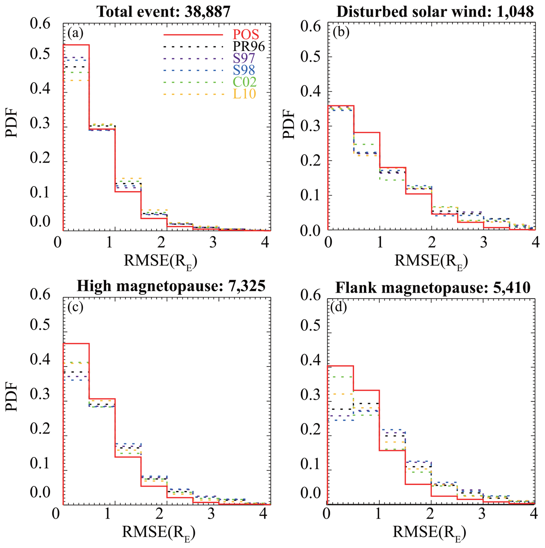
Figure 4 Distribution of models' RMSE in total (a) and under disturbed solar wind conditions (b); (c) and (d) show the prediction accuracies for the higher-latitude magnetopause region ($\left|\mathit{\theta }\right|\ge \mathrm{30}\mathit{°}$) and the magnetopause flank region ($\left|\mathit{\phi }\right|\ge \mathrm{60}\mathit{°}$), respectively.

4.1 Time-dependent feature

The models' prediction accuracies are listed in Table 3; it can be seen that all evaluated models exhibit remarkable predictive capabilities, with Δ<1R_E, aligning closely with other statistical results found in the literature (Staples et al., 2020b). It should be noted that the Δ values calculated for other models in this study may slightly differ from those reported in their original papers. This discrepancy arises due to our use of a significantly larger MCE dataset for comparison.

Table 3 Prediction accuracies of the five models and the POS for all MCEs and for MCEs under disturbed solar wind conditions.

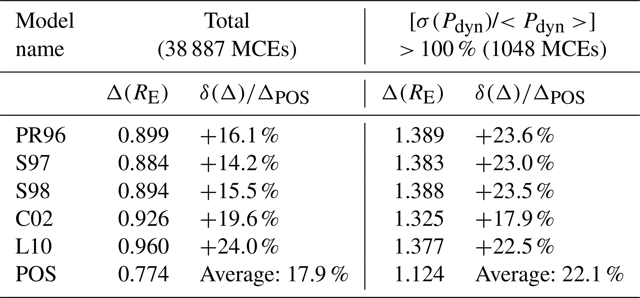
Notably, the POS model demonstrates superior predictive performance, with an average improvement of 17.9 % over the other models. Additionally, time-independent models have inherent limitations when capturing the dynamic response of the magnetosphere to solar wind fluctuations, particularly when the magnetopause standoff distance is not in phase with the P_dyn (Archer et al., 2019). In cases of highly disturbed upstream solar wind conditions, where the ratio of the standard deviation of P_dyn to the average P_dyn ($\mathit{\sigma }\left(P_{\mathrm{dyn}}\right)/<P_{\mathrm{dyn}}>$) exceeds 100 %, the POS model shows an even greater improvement in predictive accuracy, with a 22.1 % enhancement compared to other models. These results suggest that by incorporating time-dependent effects into magnetopause modelling, particularly during periods of solar wind disturbance, the POS model can more effectively capture the non-linear and out-of-phase responses of the magnetopause to rapidly changing solar wind conditions. These results also indicate that the time-dependent model represents an obvious advancement in predicting and understanding magnetospheric dynamics across a wide range of solar wind conditions.

The magnetopause is rarely static, exhibiting continuous motion under varying solar wind conditions and displaying complex dynamics during both intense disturbances and gentle changes. A notable feature of these dynamics is the periodic oscillation within the Pc5 frequency range (2–7 mHz), often termed the “magic frequency” in magnetospheric physics (Samson et al., 1992; Plaschke et al., 2009a, b). The magnetopause oscillations can be driven by quasi-periodic solar wind dynamic fluctuations or explained by magnetospheric cavity mode and Kruskal–Schwarzschild mode (Archer et al., 2013; Kruskal and Schwarzschild, 1954; Kepko and Spence, 2003; Kivelson et al., 1984). Our previous research indicates that the oscillations of the magnetopause ought to have eigenfrequencies (f₀) which are determined by the restoring force (P_B), the external driving force (P_dyn), and the damping force (P_damp) (Halliday et al., 2021; Freeman et al., 1995; Gu et al., 2023). The magnetopause will respond to solar wind conditions with phase differences ranging from 0 to 180°, depending on the driving frequency of the solar wind (f_drive). The magnetopause behaves as a low-pass filter, effectively screening out very high-frequency solar wind fluctuations (e.g. f_drive>15f₀, where f₀ is the eigenfrequency of the magnetopause). This filtering effect results in smoother predictions of magnetopause behaviour, which can be found in Fig. 5. For relatively high fluctuations (e.g. $\mathrm{15}{f}_{\mathrm{0}}>f_{\mathrm{drive}}>\mathrm{2}{f}_{\mathrm{0}}$), the phase difference between the solar wind and the magnetopause approaches 180°, indicating an anti-phase response. At resonance (f_drive≈f₀), the magnetopause exhibits a 90° phase lag relative to the solar wind forcing. Conversely, the magnetopause only behaves in-phase with the solar wind under low-frequency fluctuations (f_drive<0.5f₀), which is the scenario typically revealed by time-independent models.

The time-dependent POS model demonstrates the capability to depict these magnetospheric oscillations and the phase differences accurately. Figure 5 presents two specific cases illustrating the POS model's time-dependent performances compared with subsolar MCEs projected from THEMIS. In Case I, both models initially predict the magnetopause position at ∼ 11.5 R_E before a pressure pulse in the solar wind. The POS model uniquely predicts four oscillations around its equilibrium position (∼ 10 R_E) before the magnetopause reaches a new pressure balance. This dynamic behaviour cannot be physically captured by any time-independent models. In Case II, the POS model accurately captures the oscillations around 21:24–21:33 UT, which are not all in-phase with the solar wind dynamic pressure (P_dyn). Notably, the POS model depicts anti-phase responses observed in the second and third crossings, while the S98 model shows a reverse trend in motion, which deviates more from the observations. These results suggest that by incorporating time-dependent effects into magnetopause modelling, particularly during periods of solar wind disturbance, the POS model can more effectively capture the non-linear and out-of-phase responses of the magnetopause to rapidly changing solar wind conditions.

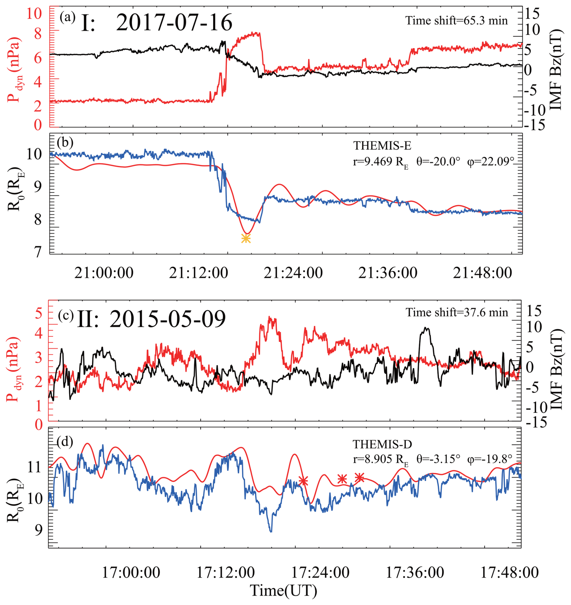
Figure 5 Case study of the overall oscillation of the magnetopause using the time-independent model S98 and the time-dependent POS model to predict its position. Panels (a) and (c) show the corresponding upstream solar wind dynamic pressure P_dyn (red line) and the interplanetary magnetic field B_z component (black line) observed by WIND with time shifts of 65.3 and 37.6 min, respectively. Panels (b) and (d) show the predictions of the S98 (blue) and the POS (red) models based on the solar wind input; the asterisks represent the subsolar positions of MCEs projected from THEMIS.

4.2 Three-dimensional characteristic

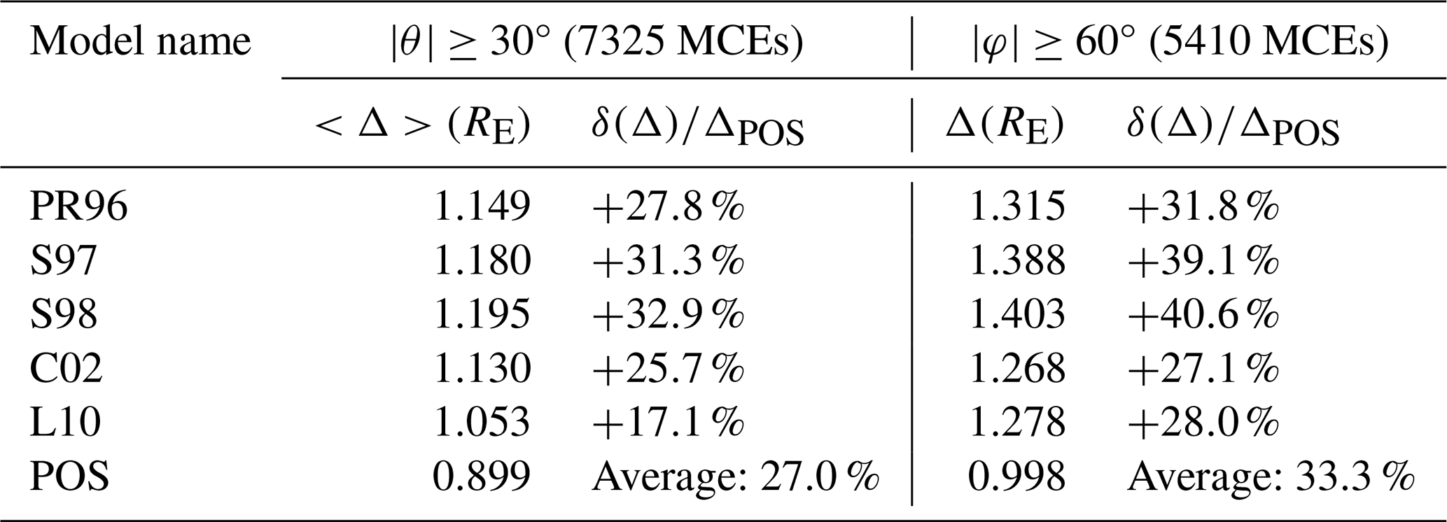
The POS model developed here incorporates the asymmetrical effects of dipole tilt angles, latitude, and longitude differences, as integrated into Eqs. (2) and (3). The model's parameters were comprehensively calibrated, allowing it to more accurately depict the three-dimensional shape of the magnetopause. To assess its validity across different magnetopause regions, extensive tests were performed, with results presented in Table 4. In the higher-latitude region of the magnetopause ($\left|\mathit{\theta }\right|\ge \mathrm{30}\mathit{°}$), a region where many models face challenges, the POS model, alongside the L10 model, demonstrates superior performance, showing an impressive 27.0 % improvement in accuracy compared to other models. Similarly, in the flank regions ($\left|\mathit{\phi }\right|\ge \mathrm{60}\mathit{°}$), where surface waves and other magnetospheric fluctuations complicate position and shape determination, the POS model maintains its high accuracy, with a 33.3 % improvement over other models. These results suggest that the POS model offers a more accurate and comprehensive representation of the magnetopause across its entire structure, outperforming other models in both higher-latitude and flank regions.

Table 4 The prediction accuracies of the five models and the POS for higher-latitude and flank regions.

Surface waves are a distinct feature of the magnetopause, originating from various factors, including the solar wind conditions, bow shock dynamics, and instabilities within the magnetopause and the magnetosphere under specific conditions. Several localized physical processes have been identified as potential drivers of these surface waves, including the Kelvin–Helmholtz instability, magnetic reconnection, and flux transfer events (Hartinger et al., 2013; Agapitov et al., 2009; Archer et al., 2021). It is also found that tailward-moving surface wavelets could be driven by disturbed solar wind conditions (large $\mathit{\sigma }\left(P_{\mathrm{dyn}}\right)/<P_{\mathrm{dyn}}>)$ (Sibeck et al., 1989). Our previous study revealed a distinct mechanism for the formation of surface-wave-like structures in the magnetopause (Gu et al., 2023). The interplay between dynamic pressure (P_dyn), magnetic pressure (P_b), and damping pressure (P_damp) results in different oscillation periods at various points on the magnetopause. These variations create a time lag within the magnetopause structure, manifesting as a surface-wave-like pattern. Figure 6 shows a surface-wave-like structure predicted by the POS model during relatively disturbed upstream solar wind conditions. The POS model's predictions are compared with those of the C02 model, which has been demonstrated as the most effective time-independent model in the flank region according to our evaluation. Figure 6 presents a specific case study illustrating the POS model's time-dependent performance compared with the positions of the THEMIS MCEs mapped to the X–Y plane. Figure 6a displays the solar wind dynamic pressure and the north–south component of the interplanetary magnetic field. The radial positions of the different points in the magnetopause in the X–Y plane (Z=0), as calculated by our model (being fully three-dimensional) exhibiting an asymmetrical flank region, are traced in Fig. 6b. Positive and negative flanks respond differently to variations in the solar wind, with discrepancies becoming more pronounced at higher φ. In this specific example, the dusk region is more significantly disturbed than the dawn region. Notably, the magnetopause shapes calculated in Fig. 6c–e reveal surface-wave-like structures evolving over time. THEMIS MCEs observed in the flank region corroborate this predicted surface-wave-like structure, indicating that the magnetopause position predicted by the POS model is more accurate than the position predicted by the C02 model.

The POS model's predictions are compared with those of the C02 model, which has been demonstrated as the most effective time-independent model in the flank region according to our evaluation. Figure 6 illustrates a surface-wave-like structure predicted by the POS model during relatively disturbed upstream solar wind conditions. The predicted surface-wave-like structure is corroborated by THEMIS MCEs in the flank region, where the actual magnetopause position is closer to Earth than the position predicted by the C02 model.

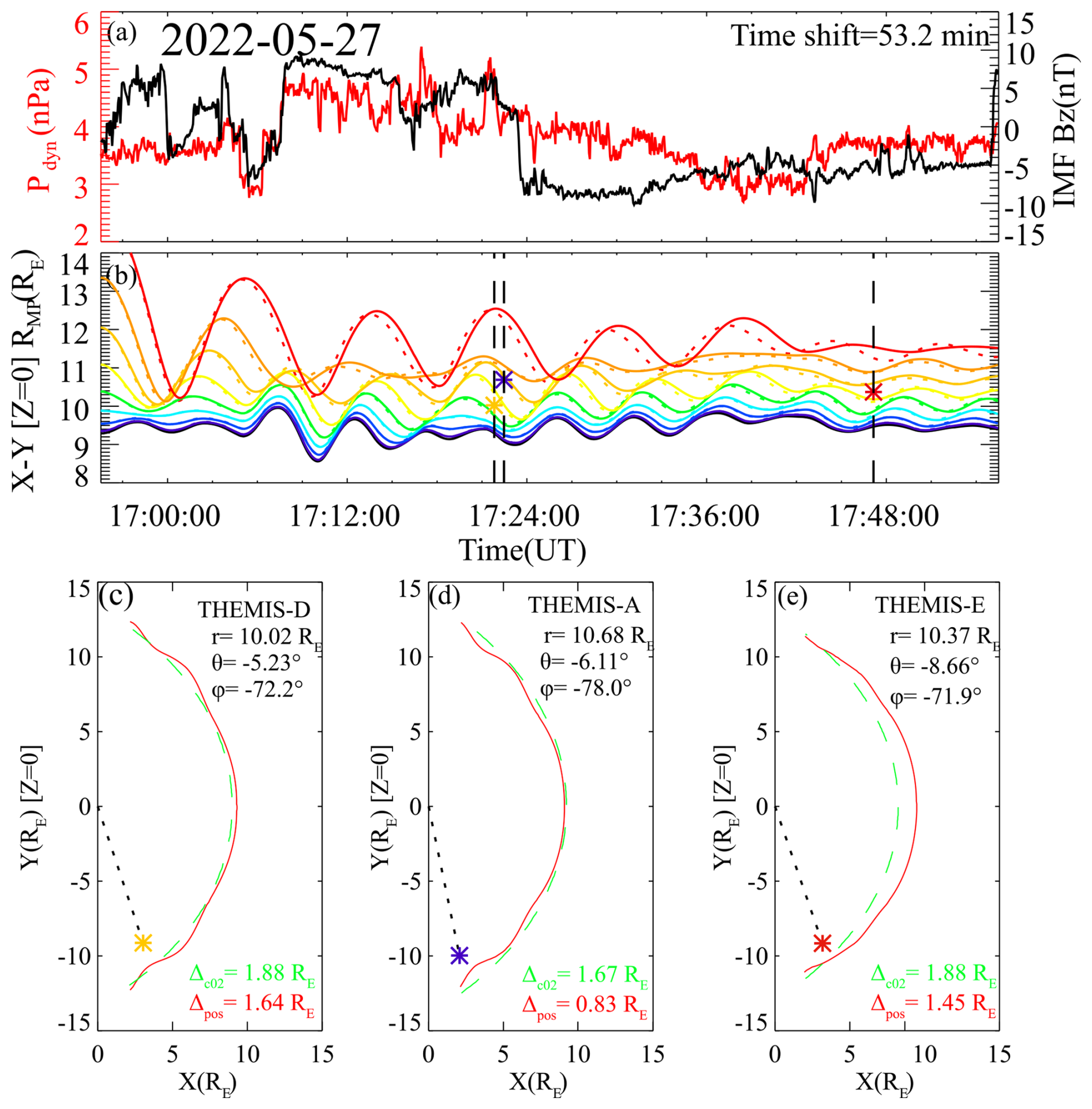
Figure 6 A surface-wave-like structure in the X–Y magnetopause flank region. Panel (a) shows the corresponding solar wind dynamic pressure (red) and IMF B_z component (black). Panel (b) shows red, orange, light orange, yellow, green, blue, dark blue, purple, and black colours representing the initial magnetopause positions at $\mathit{\phi }=\pm \mathrm{80},\pm \mathrm{70},\pm \mathrm{60},\pm \mathrm{50},\pm \mathrm{40},\pm \mathrm{30},\pm \mathrm{20},\pm \mathrm{10}$, and 0°, respectively. The dotted line indicates the corresponding negative value of φ. The asterisks in purple (THEMIS-A), yellow (THEMIS-D), and red (THEMIS-E) indicate the satellite observations of MCEs projected onto the X–Y plane. Panels (c), (d), and (e) show the shape of the magnetopause in the X–Y plane at different times predicted by the POS model (red dashed line) and the C02 model (green dotted line); the asterisks represent the THEMIS MCE positions mapped to the X–Y plane.

5 Discussion and conclusions

Accurately calculating the position of the magnetopause is essential for space weather forecasting and understanding the underlying physical mechanisms involved in the solar wind–magnetosphere interaction. In this work, we developed the POS model, the first time-dependent three-dimensional magnetopause model based on quasi-elastodynamic theory. By incorporating key solar wind parameters such as P_dyn, IMF B_z, and Φ, this model effectively depicts magnetopause dynamics. The POS model offers a new approach to describing the magnetopause position, overall oscillation, and surface-wave-like structures as interconnected phenomena. Its time-dependent feature excels in capturing dynamic processes, particularly under highly disturbed solar wind conditions. The three-dimensional nature allows for accurate depiction of the overall magnetopause shape, with notable precision in higher-latitude regions and flank areas. This capability addresses limitations in existing models and provides a more comprehensive picture of magnetopause dynamics from a different perspective. However, there are still limitations and areas for improvement that future research should address.

1. Adaptation to extreme solar wind conditions. Similar to the force–deformation relationship of a spring, which requires a specific range of applicability, the POS model has not been specifically optimized for extreme solar wind conditions (e.g. P_dyn<0.5 nPa and P_dyn>40 nPa). When the solar wind dynamic pressure is low, the quasi-elastic process between the solar wind and the magnetopause exhibits stronger damping characteristics, while at very high solar wind dynamic pressures, the magnetopause shows increased rigidity. Future iterations could incorporate more suitable damping coefficients and include P_dyn in the magnetospheric compressibility coefficient to broaden the model's applicability range.

2. Incorporation of additional solar wind factors. Existing research has shown that even under similar solar wind dynamic pressure conditions, changes in the solar wind density and velocity have distinct effects on magnetopause position (Samsonov et al., 2020). Additionally, the influence of the solar wind temperature, more comprehensive IMF effects (e.g. B_x and B_y), and other solar wind components (e.g. alpha particles) on magnetopause position are not reflected in the current model. Moreover, magnetosheath transient effects and other perturbations on the magnetopause position are not addressed (Silveira et al., 2024; Silveira and Sibeck, 2023; Sibeck et al., 2022). Future models could consider introducing these factors to achieve better predictive results.

3. Extension of the nightside magnetopause. The current POS model is primarily based on the dayside quasi-elastodynamic theory and is calibrated and validated using dayside MCEs. In the future, the model's calculation results for the nightside region could be improved by combining the fitting approach of empirical models with a more flexible curve function calibrated using a larger number of nightside MCE observations.

4. Improved representation of the cusp region. Accurately modelling the magnetopause cusp region, shaped by Earth's dipole field, remains challenging. While some models approximate this region by fitting two distinct curves, capturing its shape and position precisely is complex. Improving the representation of the cusp region will require further analysis of higher-latitude satellite data to enhance model accuracy.

5. Fine-tuning of model parameters. Further refinement of model parameters, potentially through machine learning techniques or implementing piecewise functions for different regions, could improve the model's accuracy. However, as noted in the introduction, it is important to balance model complexity with practicality. Overly complex parameter expressions can lead to increased inconvenience and higher computational costs. For those seeking the highest possible prediction accuracy, a more practical approach might involve using numerical simulations.

The upcoming SMILE mission (Solar Wind Magnetosphere Ionosphere Link Explorer), a joint mission between the Chinese Academy of Sciences and the European Space Agency, is set to launch in 2025 (Branduardi-Raymont et al., 2018; Wang and Branduardi-Raymont, 2018). This mission will provide more detailed data on magnetopause position and polar-cap shape over time, enhancing the ability to validate and refine existing magnetopause models.

In summary, this study introduces the POS model, the first time-dependent three-dimensional magnetopause model based on quasi-elastodynamic theory. Unlike time-independent models, the POS model effectively captures the dynamic movement of the magnetopause under varying solar wind conditions. When compared to five widely used models, the POS model demonstrates superior predictive accuracy, showing a 17.9 % improvement with RMSE = 0.774 R_E. As a time-dependent model, it demonstrated superior accuracy under highly disturbed solar wind conditions (22.1 % better). Its three-dimensional nature allows for enhanced accuracy in higher-latitude regions (27.0 % better) and flank regions (33.3 % better) of the magnetopause. Moreover, compared to numerical simulations, the POS model offers a concise formulation with rapid computational speed, making it feasible for direct deployment on satellites in the future – when onboard chips could complete calculations – greatly enhancing satellite intelligence. By providing a more precise and dynamic representation of the magnetopause, the POS model enhances our ability to predict and analyse space weather events and may also offer new insights and methodologies for developing magnetopause models for other planets.