Development and assessment of the physical–biogeochemical ocean regional model in the Northwest Pacific: NPRT v1.0 (ROMS v3.9–TOPAZ v2.0)

The Northwest Pacific is characterized by the presence of the warm and nutrient-depleted Kuroshio Current and the cold and nutrient-enriched Oyashio Current. In this region, surface primary production leads to increased nutrient consumption and CO₂ exchange. The Yellow and East China Seas (YECS) are predominantly influenced by freshwater input. A high resolution regional numerical model tailored to the specific features of each area is required to reproduce the different characteristics of each region. Therefore, to accurately analyze the physical and biogeochemical system, this study developed a new coupled physical–biogeochemical model combining the three-dimensional Regional Ocean Modeling System (ROMS) and the Generic Ocean Turbulence Model Tracers of Phytoplankton with Allometric Zooplankton (TOPAZ) for the Northwest Pacific, including the YECS. The simulated physical and biogeochemical variables in the ROMS–TOPAZ (NPRT) were evaluated by comparing them with available observational data. NPRT successfully simulated the seasonal variability of chlorophyll and nutrients, capturing two peaks in spring and autumn that were not captured by the CMIP6 data. Particularly in the YECS, NPRT effectively represented the high phytoplankton biomass driven by the riverine effect, which is difficult to reproduce in global biogeochemical models with low-resolution. However, NPRT still exhibits significant biases in the subarctic region and marginal seas. To minimize the uncertainties in biogeochemical variables, it is necessary to refine the initial and boundary conditions, adjust parameters, and apply discharge forcing based on observational data. Despite these limitations, NPRT is an important tool for studying the interaction between ocean physics and biogeochemistry at a high resolution.

1 Introduction

Ocean biogeochemical processes are among the most important fields for understanding Earth's carbon and ecosystem cycles, as well as the global climate system (Reid et al., 2009; Kang et al., 2017; Park et al., 2014; 2018, Lee et al., 2022). Previous studies utilized Earth system models to analyze ocean biogeochemistry, climate feedback, and the carbon cycle (Kang et al., 2017; Park et al., 2018, 2019). In particular, significant efforts have been made to analyze physical–biogeochemical features at the global scale as well as at regional scales (Hauri et al., 2020; Zhao et al., 2021; Wu et al., 2023; Na et al., 2024).

The North Pacific is a key region where the biological carbon pump occurs effectively (Chierici et al., 2006; Takahashi et al., 2009). Low-frequency physical and ecological variabilities in the North Pacific are closely related to various climatological variability patterns, such as the Pacific Decadal Oscillation (PDO) and El Niño–Southern Oscillation (ENSO). Numerous studies have been conducted on the responses of ecosystems to climatic and environmental conditions influenced by these long-term climatological variability patterns, especially in the Northeast Pacific (Overland et al., 2008; Yatsu et al., 2013; Ma et al., 2020). However, in the Northwest Pacific, including marginal seas, regional-scale oceanographic and ecological variabilities are independent across regions and show relatively weak linkages to climatological variability patterns, such as the PDO and ENSO (Jung et al., 2017; Ma et al., 2020). In particular, the Northwest Pacific is known as the Kuroshio–Oyashio Confluence Region (142–160° E, 35–40° N; Kawai, 1972; Hanawa and Mitsudera, 1987); the Oyashio Current is formed from the East Kamchatka Current, flowing southwestward along the Hokkaido coast while mixing with the Okhotsk Sea Mode Water, and the Kuroshio Current flows northeastward along the east of Japan, originating from Luzon Island (Nitani, 1972). Therefore, this region is known for the convergence of distinct water properties, resulting in a complex frontal structure, thermohaline mixing, and significant variability in the upper layer circulation (Qiu, 2001; Yasuda, 2003; Taguchi et al., 2007). Specifically, the water mass of the Oyashio Current has low temperature and low salinity, i.e., lower than 7 °C and 33.7 psu at a depth of 100 m (Kawai, 1972). Conversely, the water mass of the Kuroshio Current has a temperature higher than 14 °C and salinity higher than 34.7 psu (Nitani, 1972; Wang et al., 2022). In this region, the biogeochemical characteristics also exhibit significant regional differences. The cyclonic subarctic gyre, located west of the Oyashio Current, is characterized by high nutrient levels and low chlorophyll concentration (Taniguchi, 1999). Conversely, the anticyclonic tropical gyre, situated in the Kuroshio Current, is characterized by low nutrient levels (Siswanto et al., 2015). The interaction between gyres with distinct biogeochemical characteristics results in increased nutrient availability and the simulation of high phytoplankton biomass (Shiozaki et al., 2014). Consequently, the Northwest Pacific has been extensively studied from the perspectives of hydrography, climate change, nutrient transport, the carbon cycle, phytoplankton production, and community structure in relation to external conditions (Okamoto et al., 2010; Kuroda et al., 2019; Wang et al., 2021).

The Northwest Pacific is an important region for understanding the global carbon cycle and enhancing its predictability. Many previous studies have analyzed the carbon cycle, ecosystems, and future climate change using low-resolution global climate models with biogeochemical modules (Park et al., 2014; Jung et al., 2020; Hauri et al., 2020; Lee et al., 2022). However, coupled physical–biogeochemical ocean models with low horizontal resolutions involve limitations regarding accurately reproducing and analyzing the characteristics of oceanic environmental systems – particularly in the physical–biogeochemical factors in regional areas. Therefore, in this study, to accurately understand the physical–biogeochemical processes at the regional scale and address uncertainties, a regional ocean model and a biogeochemical model were coupled at a high resolution. Specifically, we employed the Generic Ocean Turbulence Model–Tracers of Phytoplankton with Allometric Zooplankton (TOPAZ) developed by the US National Oceanic and Atmospheric Administration's Geophysical Fluid Dynamics Laboratory (GFDL) in conjunction with the Regional Ocean Modeling System (ROMS).

This study introduces a new high-resolution coupled physical–biogeochemical model, named the “Northwest Pacific ROMS–TOPAZ model version 1.0 (hereafter NPRT)”, which is a valuable tool for not only understanding the interactions between physical and biogeochemical processes but also for predicting the future ocean carbon system. We describe and evaluate the simulation results of the coupled physical–biogeochemical model (NPRT) through comparison with available observational data. Section 2.1 and 2.2 describe the characteristics of the models used in this study and Sect. 2.3 and 2.4 elaborate on the developed NPRT, the methodology behind it, and the specific model design for the study area. In Sect. 3, the model results are evaluated using observations of physical and biogeochemical variables, such as sea surface height (SSH), salinity, chlorophyll, nutrients, dissolved inorganic carbon (DIC), alkalinity (Alk), and dissolved oxygen (DO). In addition, we analyze the characteristics of the physical–biogeochemistry regional ocean model with high resolution. Finally, a summary is presented in Sect. 4.

2 Data and model

2.1 Physical Ocean model (ROMS v3.9)

For conducting the physical–biogeochemical model coupling in this study, we employed ROMS version 3.9 (hereafter ROMS; Song and Haidvogel, 1994), which is a popular physical regional ocean model. ROMS is a three-dimensional primitive-equation physical ocean model that uses hydrostatic and Boussinesq approximations. The horizontal grid system is the Arakawa-C grid system, which enhances computational stability and efficiency (Arakawa and Lamb, 1977). The vertical coordinate system is the S-coordinate (stretched terrain-following coordinate), which combines the advantages of implementing the z-coordinate for the planetary boundary layer (PBL) and the σ-coordinate for the bottom boundary layer. In this way, it allows for accurate analyses of physical phenomena in the thermocline or bottom boundary layer, while reducing pressure gradient errors that are sensitive to the terrain (Song and Wright, 1998; Shchepetkin and McWilliams, 2003).

ROMS can utilize horizontal advection schemes, such as second-, and fourth-order centered differences and a third-order upstream scheme. Various options are available for vertical mixing, including the K-profile parameterization (KPP; Large et al., 1994), M–Y (Mellor and Yamada, 1982), generic length scale (GLS; Umlauf et al., 2003). In addition, bulk parameterization involving the wind, sensible heat flux, and latent heat flux provides better calculations of the heat budget changes, which is essential for elucidating the atmosphere–ocean interactions (Fairall et al., 1996). For more information on ROMS, we refer to Shchepetkin and McWilliams (2005) and McWilliams (2009).

2.2 Biogeochemical model (TOPAZ v2.0)

TOPAZ version 2.0 (hereafter TOPAZ) is a biogeochemical module that simulates the cycles of carbon, nitrogen, phosphorus, silicon, iron, DO, and lithogenic material, while also considering the growth cycles of the zooplankton and phytoplankton. In biogeochemical processes, phytoplankton members are categorized based on their sizes into small and large, including the nitrogen-fixing diazotrophs. Overall, TOPAZ handles a total of 30 prognostic and 11 diagnostic tracers. The state variable C in various tracers reproduced in TOPAZ can be calculated using the following continuity equation to describe local changes.

$$\begin{array}{}\text{(1)}& {\displaystyle \frac{\partial C}{\partial t}}=-\mathrm{\nabla }\cdot \stackrel{\mathrm{̃}}{v}C+\mathrm{\nabla }K\mathrm{\nabla }C+S_{\mathrm{c}},\end{array}$$

where $\stackrel{\mathrm{̃}}{v}$ and K represent the vector velocity and diffusivity, respectively, and S_c indicates the source-minus-sink terms of the state variable C calculated at each grid. TOPAZ considers eight types of biogeochemical processes: the dissolved organic matter (DOM) cycle, particle sinking, dry/wet atmospheric decomposition, gas exchange, river input, removal, sediment input, and scavenging (Dunne et al., 2005, 2007). Various equations for these processes are available, utilizing relationships between variables derived from observational data (Dunne et al., 2012). In addition, TOPAZ includes an “optical feedback” module that considers the chlorophyll photosynthesis. Optical feedback calculates the total surface irradiance (I(z)) as a function of the solar radiation wavelength (Manizza et al., 2005). This scheme regulates vertically penetrating irradiance due to shortwave radiation absorption in the visible light, which is influenced by the distribution of chlorophyll concentration in the water column of the model.

$$\begin{array}{}\text{(2)}& \begin{array}{rl}I\left(z\right)=& I_{\text{IR}}\cdot e^{-k_{\text{IR}}^{\mathrm{2}}}+I_{\text{RED}(z-\mathrm{1})}\cdot e^{-k_{\left(r\right)}\mathrm{\Delta }z}\\ & +I_{\text{BLUE}(z-\mathrm{1})}\cdot e^{-k_{\left(b\right)}\mathrm{\Delta }z},\end{array}\end{array}$$

where the first term in the right hand side represents the penetration of the infrared wavelength band, and the second and third terms represent the photosynthetically active radiation (PAR), which is divided into two visible wavelength bands, namely the red and blue/green bands. PAR is used to calculate the growth rate of phytoplankton groups and is a key factor in biogeochemistry. For more detailed information on TOPAZ, we refer to Dunne et al. (2012).

In the TOPAZ model, there are not only the primary 11 diagnostic variables but also many secondary diagnostic variables. Net primary production (NPP) was calculated using the secondary diagnostic variables such as the maximum growth rate, temperature, nutrients, and light limitation factors (Laufkötter et al., 2015). Unfortunately, the TOPAZ model used in this study does not store secondary diagnostic variables related to NPP. Nevertheless, since it simulates various nutrients, chlorophyll concentrations, and carbon cycles, the TOPAZ model can be effectively used to analyze biogeochemical processes.

2.3 The coupled ROMS–TOPAZ model (NPRT version 1.0)

In this study, to couple ROMS with TOPAZ, we employed the stand-alone version of TOPAZ, which was separated from the Modular Ocean Model version 5 (MOM5) developed by the GFDL in a previous study (Jung et al., 2020). For the stand-alone version of TOPAZ, the air–sea gas exchange for CO₂ and O₂ is based on Wanninkhof (1992) and Najjar and Orr (1998) and the optical feedback is based on Manizza et al. (2005). In addition, TOPAZ forces the surface fluxes of nutrients from the atmosphere to the ocean for nitrate (NO₃), ammonia (NH₄), lithogenic aluminosilicate (LITH), and dissolved iron (Fed) (Jung et al., 2020). For these atmospheric chemistry values for the surface flux, this study employs climatological monthly mean data as provided by the official MOM GitHub (https://mom-ocean.github.io/docs/quick-start-guide/, last access: 1 March 2023).

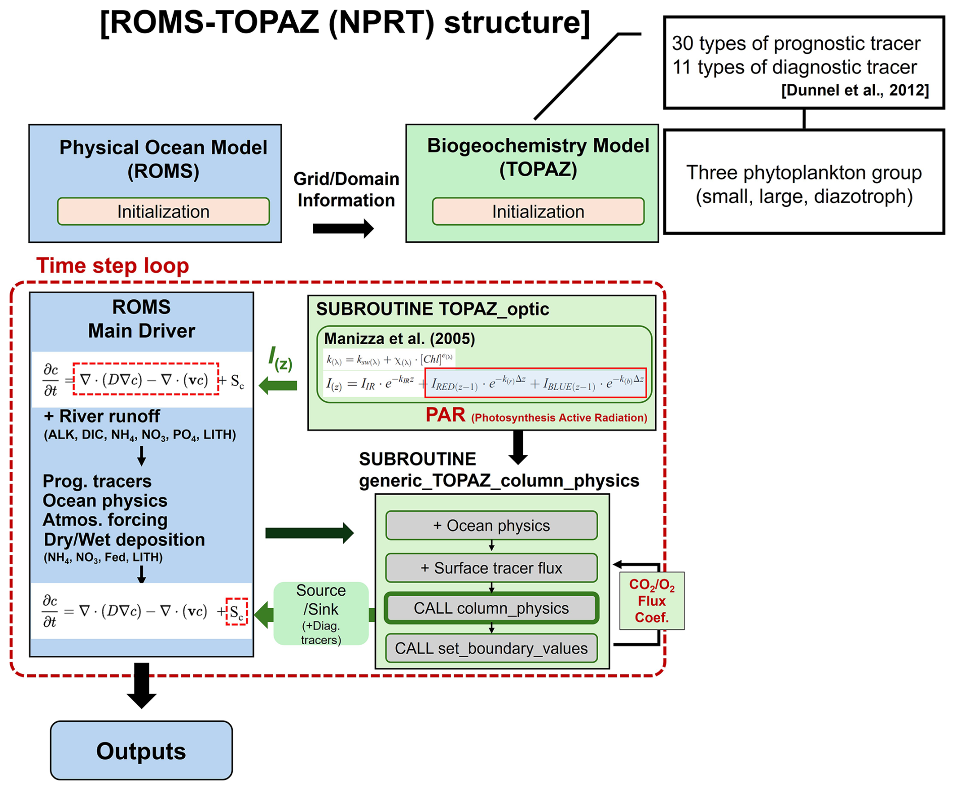
Figure 1 Flow diagram of the ROMS–TOPAZ model (NPRT). Blue and green boxes represent the ocean physical and biogeochemical modules, respectively. The black arrows indicate the process of transferring oceanic physical information to biogeochemical modules and the green arrows represent the vice versa process.

Figure 1 shows the structure of the NPRT. During the initialization process, TOPAZ receives the grid and domain information from ROMS. Subsequently, integration with the ROMS Main Driver occurs to calculate S_c within the “time step loop” using Eq. (1). Simultaneously, the chlorophyll optical feedback is also considered in each time step, with the PAR modified by chlorophyll concentrations influencing S_c, whereas the total radiation is used in the physical processes of ROMS. In the ROMS Main Driver, the advection and diffusivity terms are calculated considering river runoff (Alk, DIC, NH₄, NO₃, LITH, and PO₄). Information such as prognostic tracers, ocean physical variables, atmospheric forcing, and dry/wet deposition (LITH, NH₄, NO₃, and Fed) are then transmitted to the TOPAZ module, where the source/sink term (S_c) is calculated. In other words, the state variable C is calculated using data related to the transport tendency of the tracers and source/sink term through the ROMS physics and generic_TOPAZ_column_physics modules (Fig. 1).

2.4 Experimental setup

To operate NPRT, it is necessary to obtain the initial and boundary conditions for the biogeochemical variables considered by TOPAZ; however, it is impossible to encompass all biogeochemical observational data, since TOPAZ considers 30 prognostic and 11 diagnostic tracers. Therefore, in this study, the results of MOM5–TOPAZ were employed as the initial and boundary conditions of TOPAZ. To operate MOM5–TOPAZ, the default input datasets provided by the official MOM GitHub were employed for the initial condition. MOM5–TOPAZ was initially operated for a 100 year spin-up integration under a pCO₂ environment (369.6 ppm) and ECMWF Reanalysis v5 (ERA5; Hersbach et al., 2020) of year 2000. Séférian et al. (2016) suggested that biochemical models require spin-up times longer than those required by physical ocean models. However, in this study, we adopted a 100 year spin-up time integration because of limited computing and time resources. After the 100 year spin-up time integration, using the results from the last time step as the initial condition, MOM5–TOPAZ was operated for 2000–2014, with a realistic atmospheric CO₂ concentration and atmospheric forcings from ERA5. Through these spin-up process described above, the initial and boundary conditions for the biogeochemical variables required to conduct NPRT were obtained. Nutrient concentrations for dry/wet atmospheric deposition and runoff were obtained from the default input data of the official MOM GitHub.

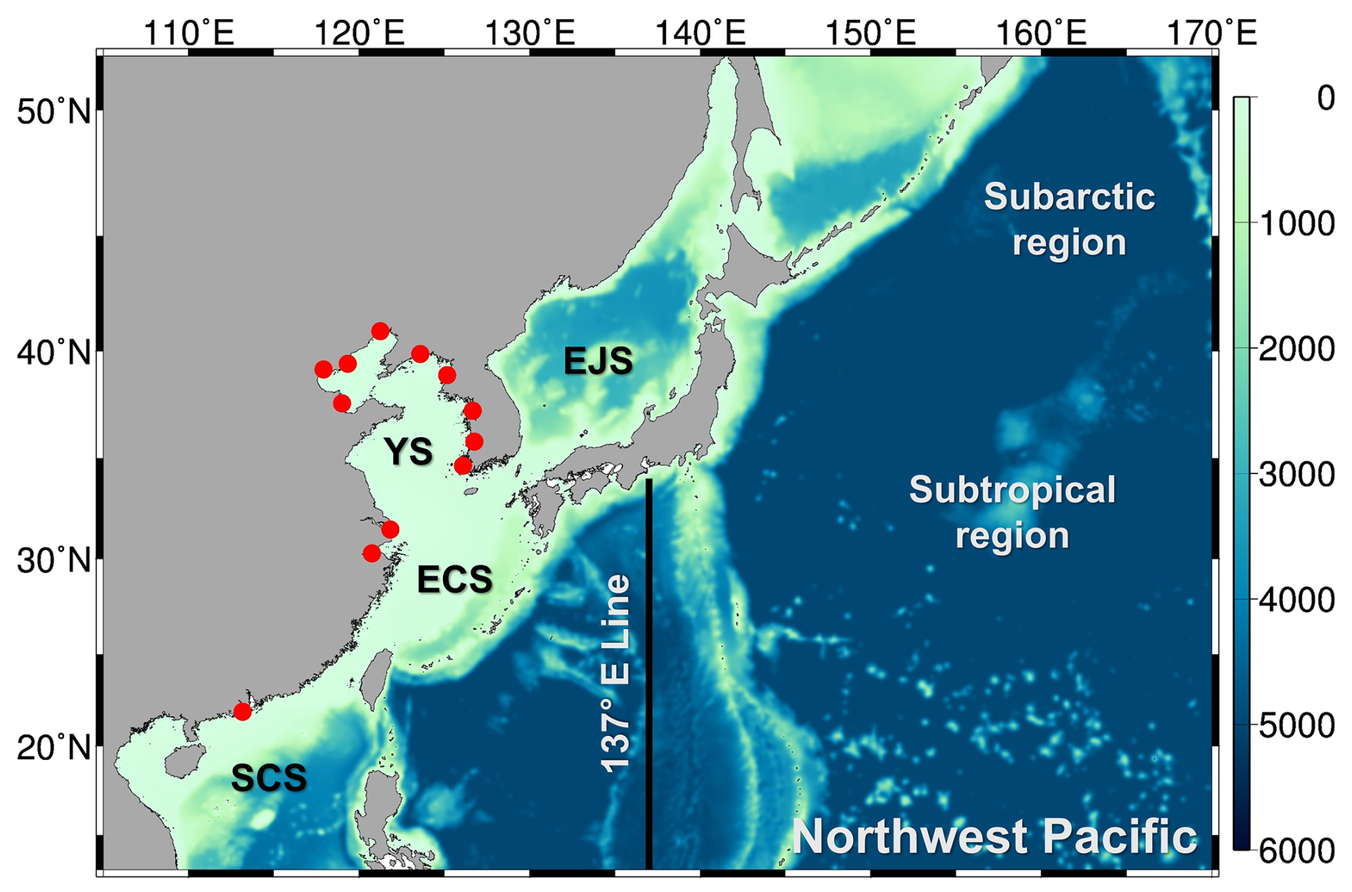
Figure 2 Model domain and bottom topography for NPRT coupled modeling system. EJS: East/Japan Sea, YS: Yellow Sea, ECS: East China Sea, SCS: South China Sea. The red circles indicate river runoff points and the black line (137° E line) is the observation line of the Japanese Meteorological Agency (JMA).

The initial and boundary conditions used for the physical variables were monthly mean data from the Hybrid Coordinate Ocean Model (HYCOM; Bleck, 2002) reanalysis with a $\mathrm{1}/\mathrm{12}$° (approximately 8 km) horizontal resolution. We used the six-hourly atmospheric external forcings, as provided by ERA5, as well as climatological monthly mean discharges of 12 major rivers, including the Yangtze, Huanghe, Yungsan, Keum, Han, Haihe, Luanhe, Amnokgang, Taedong, Qiantang, and Pearl rivers (Fig. 2; Kwon, 2007). In addition, to obtain the tidal mixing effect, we considered 10 major tidal and tidal current harmonic components (M₂, S₂, N₂, K₂, K₁, O₁, P₁, Q₁, M_f, and M_m) from TPX07 (Egbert and Erofeeva, 2002). The GLS vertical mixing scheme was used for parameterization (Umlauf et al., 2003). The bottom stress is parameterized with a quadratic drag law using a drag coefficient (2.5 × 10⁻³); horizontal viscosity and diffusion coefficients are 25 and 50 m² s⁻¹, respectively.

In this study, the model domain (13–52° N, 105–170° E) is the Northwest Pacific (NWP), which is one of the key regions for conducting global air–sea gas exchange, and includes the East/Japan Sea (hereafter East Sea), the Yellow and East China Seas (YECS), and South China Sea (Fig. 2). The horizontal resolution is $\mathrm{1}/\mathrm{12}$°, both in longitude and latitude, and the number of vertical layers is 50. The bottom topography from GEBCO data (Weatherall et al., 2015) is interpolated onto the model grid. NPRT was operated for a total of 15 years (2000–2014). To address the requirement for a sufficiently long spin-up time for executing the biogeochemical model, we conducted an additional spin-up for the initial five years. Therefore, in this study, the model results averaged over the last 10 years were used for the analysis.

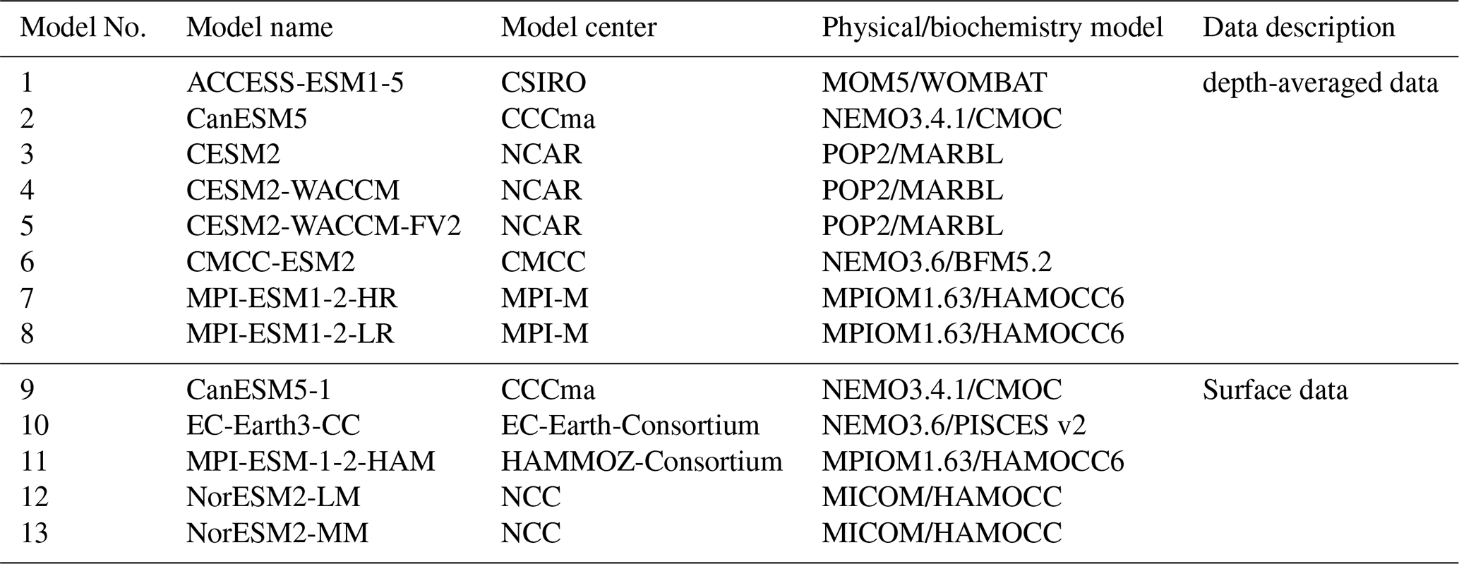
Table 1 CMIP6 Earth system models were used in this study for comparison with chlorophyll concentration.

To compare NPRT simulations with available observational data, in this study we divided the Northwest Pacific into four regions on the base of physical and biological environments: the NWP, further subdivided into subtropical (south of 40° N) and subarctic regions (north of 40° N), the East Sea, and the YECS (Fig. 2). The SSH distribution was obtained from the Copernicus Marine Environment Monitoring Service (CMEMS) satellite data from 2005–2014. Sea water temperature and salinity are not only key factors in phytoplankton growth but also essential physical factors that determine the water mass distribution in the ocean. In this study, the water temperature and salinity simulated from NPRT were verified via annual and monthly climatological datasets from the World Ocean Atlas 2018 (WOA18) at a horizontal resolution of 1° × 1°. In addition, to evaluate the reproducibility of chlorophyll concentrations, the Moderate Resolution Imaging Spectroradiometer (MODIS; Barnes et al., 1998) and the Coupled Model Intercomparison Project phase 6 (CMIP6; Eyring et al., 2016) were employed. As shown in Table 1, this study adopted six models from CMIP6, providing chlorophyll concentrations for the historical period (2005–2014). Each model is a single ensemble member, typically the “r1i1p1f1” model: r, i, p, and f denote the realization, initialization, physics, and forcing indices, respectively (Taylor et al., 2018). For dissolved oxygen and nutrients, we also used annual and monthly climatological datasets from WOA18. In addition, we utilized conductivity–temperature–depth (CTD) measurement data such as DO, from the Japan Meteorological Agency (JMA) along the 137° E line from 2005–2014. The simulated DIC and alkalinity in NPRT was compared with observational data from the Global Ocean Data Analysis Project version 2 (GLODAPv2; Lauvset et al., 2016) with a horizontal resolution of 1° × 1° and 33 vertical layers from 0 to 5500 m. GLODAPv2 is the mapped climatology field averaged from 1972–2013 at the Carbon Dioxide Information Analysis Center (CDIAC).

3 Results and discussion

3.1 Physics

The study area is characterized by diverse oceanic environments that determine the biogeochemical characteristics. For example, in the Kuroshio–Oyashio Confluence Region, the distributions of biogeochemical variables are determined by various physical and biological processes, such as advection, horizontal mixing, vertical mixing, photosynthesis, and respiration. In addition, the YECS is a river-dominated marginal sea, where large amounts of nutrients are discharged into the sea along with freshwater (Dai et al., 2022; Na et al., 2024). Therefore, to accurately simulate the biogeochemical properties, validating the oceanic physical characteristics, such as water temperature, current, and salinity, is necessary. The distribution of ocean currents, in conjunction with water temperature and salinity, is essential for determining the oceanic physical characteristics. This key factor plays a fundamental role in direct and indirect assessments of all aspects of the marine environment. To validate the reproducibility of the physical characteristics, the simulated SSH data were compared with satellite-observed altimetry data from CMEMS.

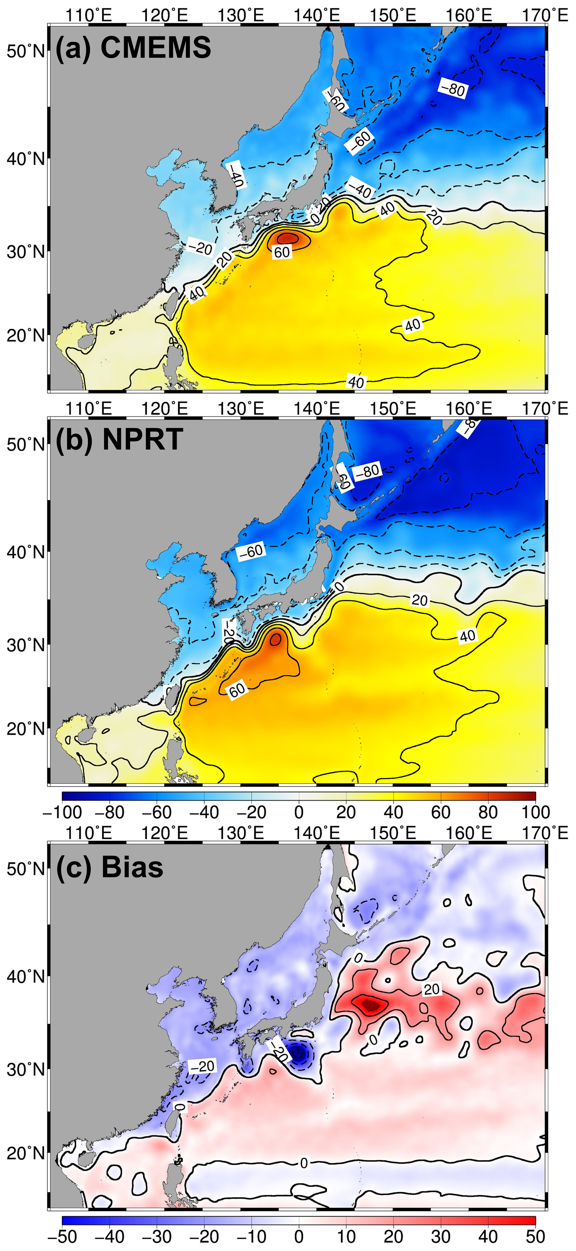
Figure 3 Distributions of the annual mean sea surface height (SSH; cm) in (a) satellite altimeters (CMEMS), (b) NPRT, and (c) biases between NPRT and observations (WOA18) from 2005 to 2014. To compare the two datasets, the spatial mean was subtracted from each one.

Figure 3 shows the long-term mean SSH distributions in CMEMS and NPRT during 2005–2014. The Kuroshio Current originates from east of the Philippine coast, where it flows northeastward, passes through the Tokara Strait, and continues eastward, meandering along the southern coast of Japan. Furthermore, in the Shikoku Basin, there is a long-standing anticyclonic eddy associated with ocean-bottom topography (Ding et al., 2022). In the subarctic region, the Oyashio Current flows southward and converges with the Kuroshio Current, resulting in the mixing of distinct water masses; the region where this happens is known as Kuroshio–Oyashio Confluence Region (Sugimoto and Hanawa, 2011; Zhu et al., 2019). As mentioned previously, the NPRT results generally agree well with the observed characteristics of the upper-layer circulation system in the NWP.

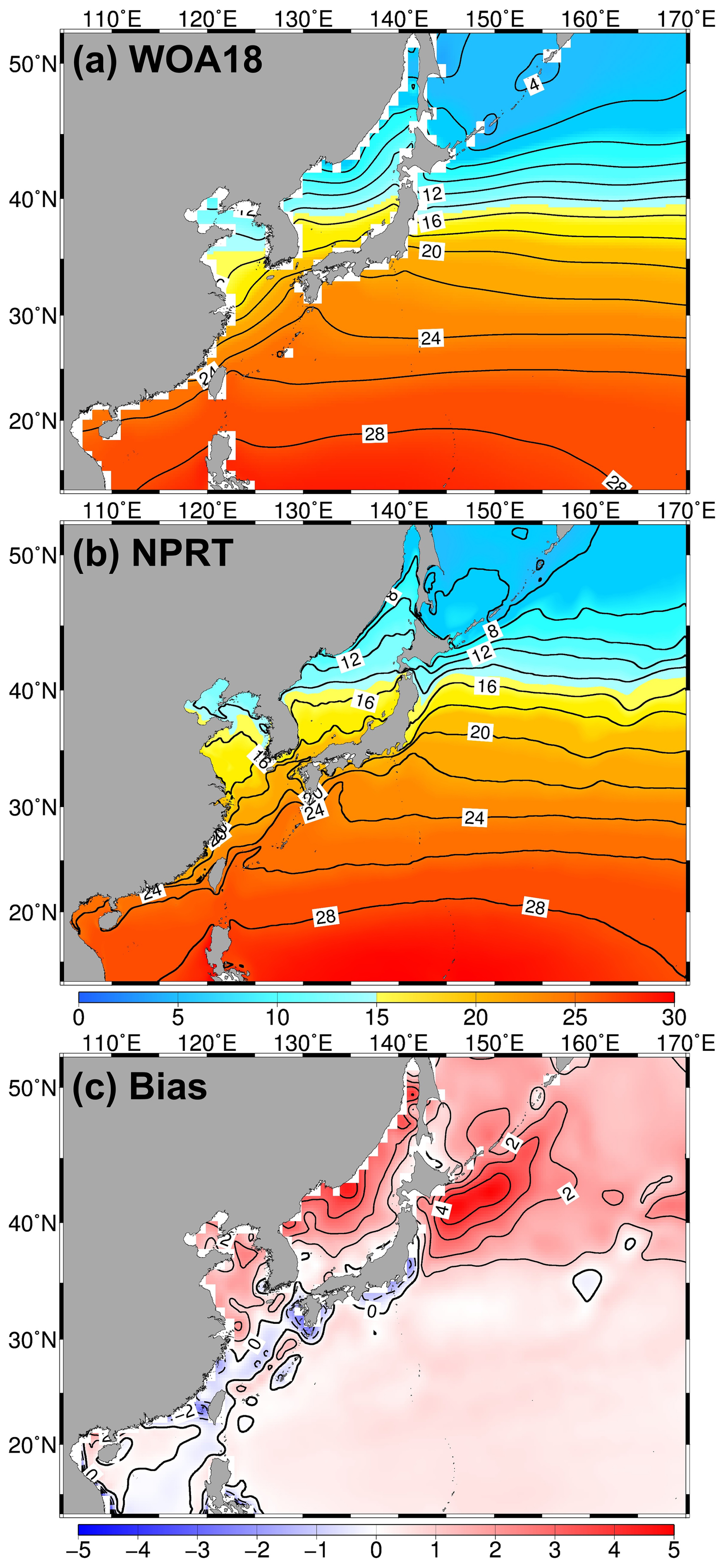
Figure 4 Same as Fig. 3 but applied to in the annual mean sea surface temperature (SST) from (a) World Ocean Atlas 2018 (WOA18), (b) NPRT, and (c) bias (NPRT – WOA18).

Figure 4 shows the annual mean sea surface temperature (SST) in WOA18 and NPRT. The Northwest Pacific exhibits subtropical characteristics, with high temperatures above 25 °C typical at approximately 20° N. Additionally, this region is predominantly influenced by the Kuroshio Current with its warm water mass, which results in the northward distribution of isotherms along the Japanese coast. As mentioned above, a significant north–south temperature gradient is also observed between 35 and 40° N, corresponding to the Kuroshio–Oyashio Confluence Region. The characteristics of the SST distribution in the Northwest Pacific are highly pronounced in NPRT, although the simulated sea surface temperature predominantly shows a positive bias, with a particularly significant positive bias (> 4 °C) observed in the Kuroshio–Oyashio Confluence Region (Fig. 4c). Notably, the location of the Kuroshio–Oyashio Confluence Region, which plays a crucial role in the formation of the North Pacific Intermediate Water (NPIW), is also accurately simulated.

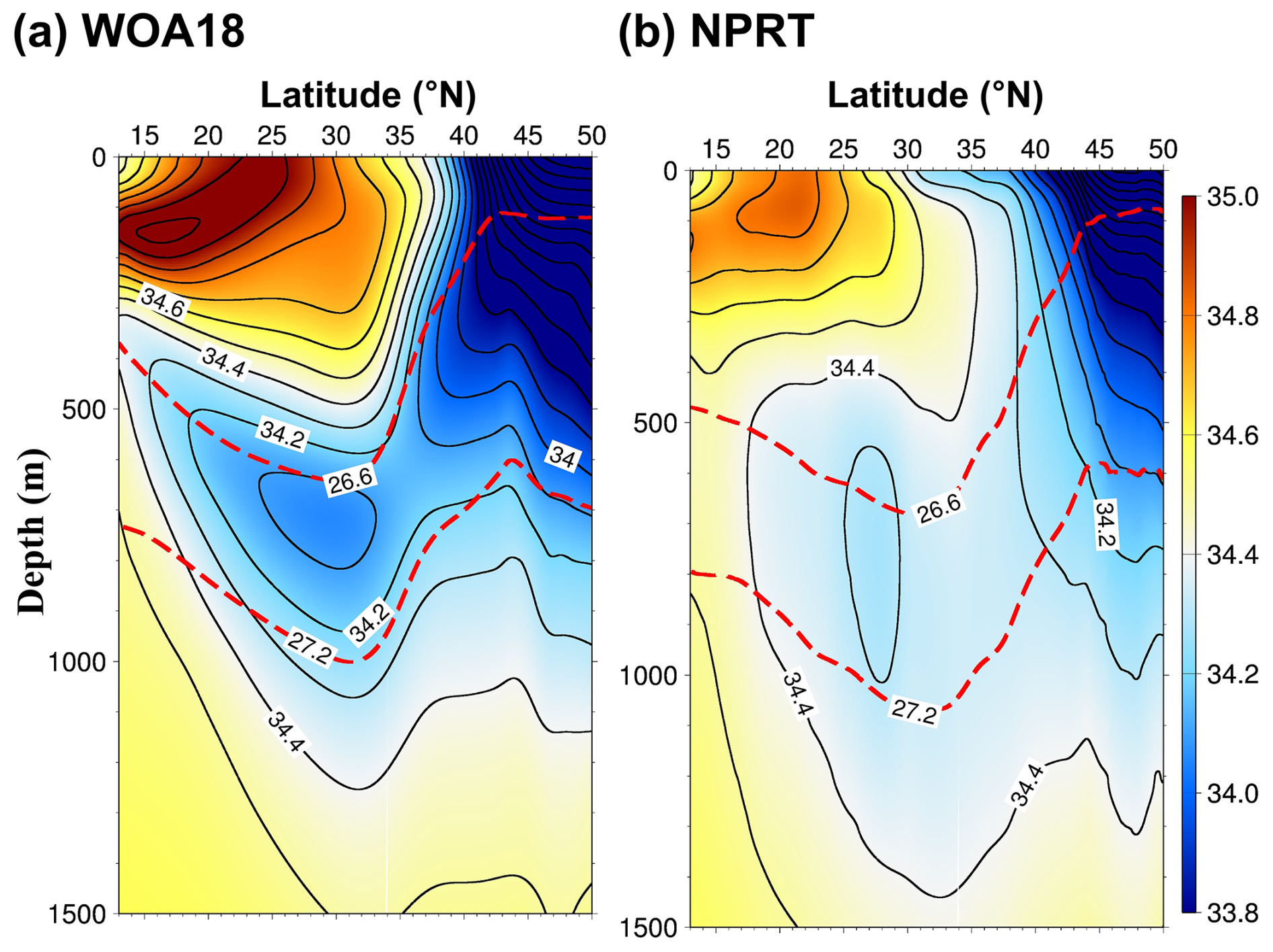
Figure 5 Vertical structures of the climatological zonally averaged annual mean salinity between 145 and 160° E in (a) the WOA18 data and (b) NPRT. The red dashed lines represent potential 26.6 and 27.2 σ_θ isopycnals, corresponding to the NPIW density range.

The NPIW is characterized by salinity and potential vorticity minima, with its salinity minimum layer primarily distributed between density 26.6 and 27.2 σ_θ, corresponding to depths of 600–800 m (Lembke-Jene et al., 2017). The NPIW transports large amounts of nutrients to the NWP. Therefore, simulating the NPIW is important for the reproduction of biogeochemical characteristics in the NWP. Comparing the vertical structures of zonal mean salinity between 140 and 160° E to those in the WOA18 data shows that the depth of the salinity minimum layer is approximately 600–800 m, similar to the observational data (Fig. 5). However, the salinity minimum layer is about 0.2 psu higher than that of the observations. This is attributed to a significant positive bias of salinity simulated in NPRT in Kuroshio–Oyashio Confluence Region. Nevertheless, NPRT adequately reproduces not only the surface currents but also the ventilation for the formation of the NPIW.

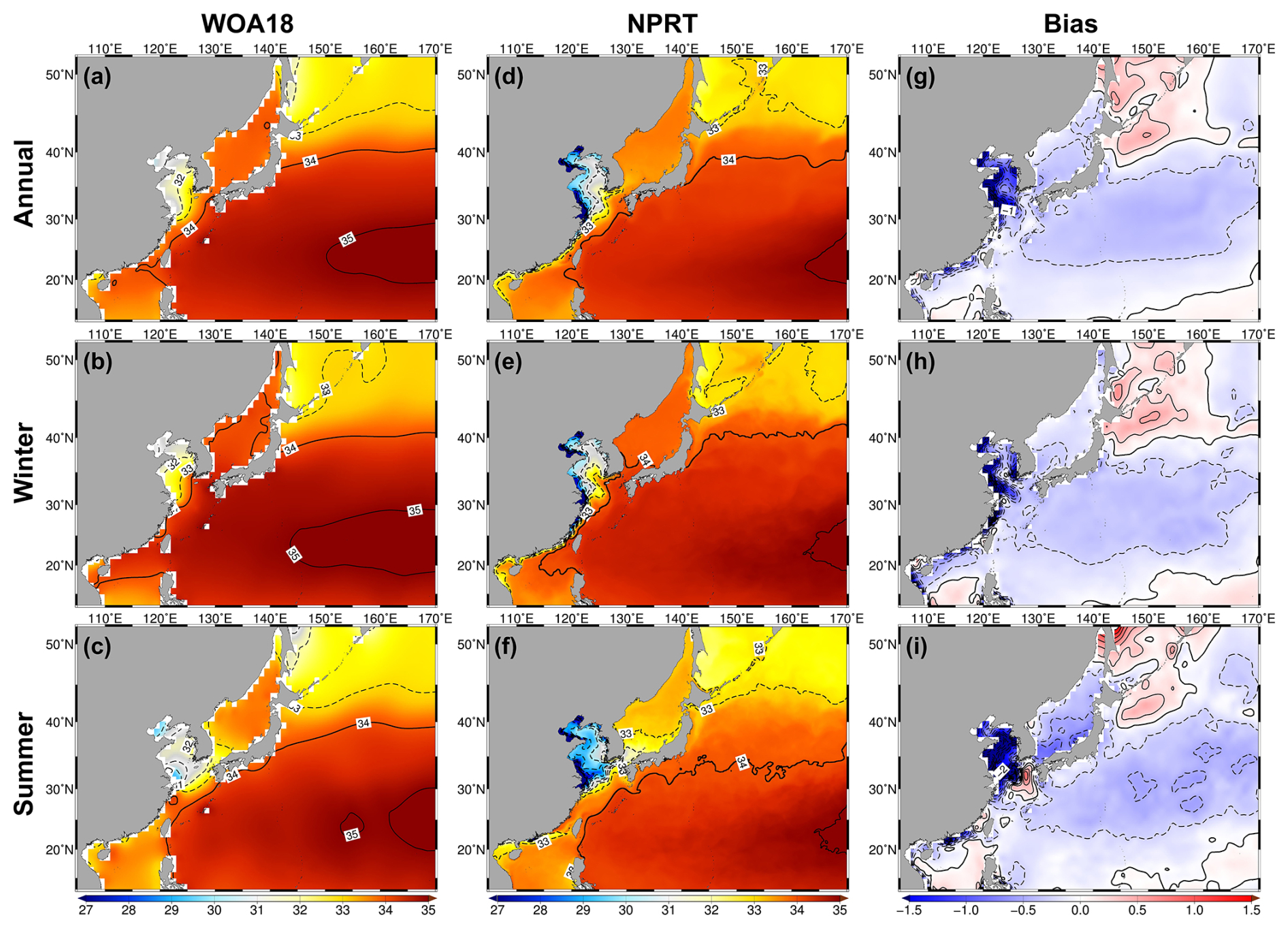
Figure 6 Distributions of the surface salinity in (a–c) the WOA18 data, (d–f) NPRT, and (g–i) biases for (a, d, g) the climatological mean, (b, e, h) winter, and (c, f, i) summer.

The YECS are characterized by the dominant effects of tidal mixing and runoff. Freshwater discharged from the Yangtze River, one of the major sources of nutrients in the East China Sea, forms a low-salinity plume that spreads and influences the stratifications of the surrounding areas (Moon et al., 2009). NPRT did not include all rivers in the YECS; nevertheless, a total of 12 rivers, including the Yangtze River, were included (Fig. 2). Regarding the oceanographic characteristics of the YECS, the model exhibits similar patterns with those of the observations from WOA18, despite a negative bias (Figs. 6 and S1 in the Supplement). During winter (February; Figs. 6e and S1e), the simulated sea surface salinity distribution in the YECS is below 32.0 psu, whereas during the freshwater discharge-intensive summer (August; Figs. 6f and S1f), the salinity drops below 30 psu, forming a low-salinity tongue shaped feature extending toward the Korean coast. In the NWP, high salinity water (> 34.0 psu) extends northward to around 40° N during winter and around 35° N during summer. The reproduced distinct seasonal variability is similar to that in the WOA18 data, with all spatial correlation coefficients and root-mean-square error (RMSE) for surface salinity distribution in the annual mean, winter, and summer being over 0.93 and 0.33–0.42 psu, respectively.

Overall, NPRT reasonably simulates the major characteristics observed in each region and is, therefore, suitable for analyzing the spatiotemporal distribution and characteristics of chlorophyll concentration, nutrients, and the carbon cycle influenced by these physical properties.

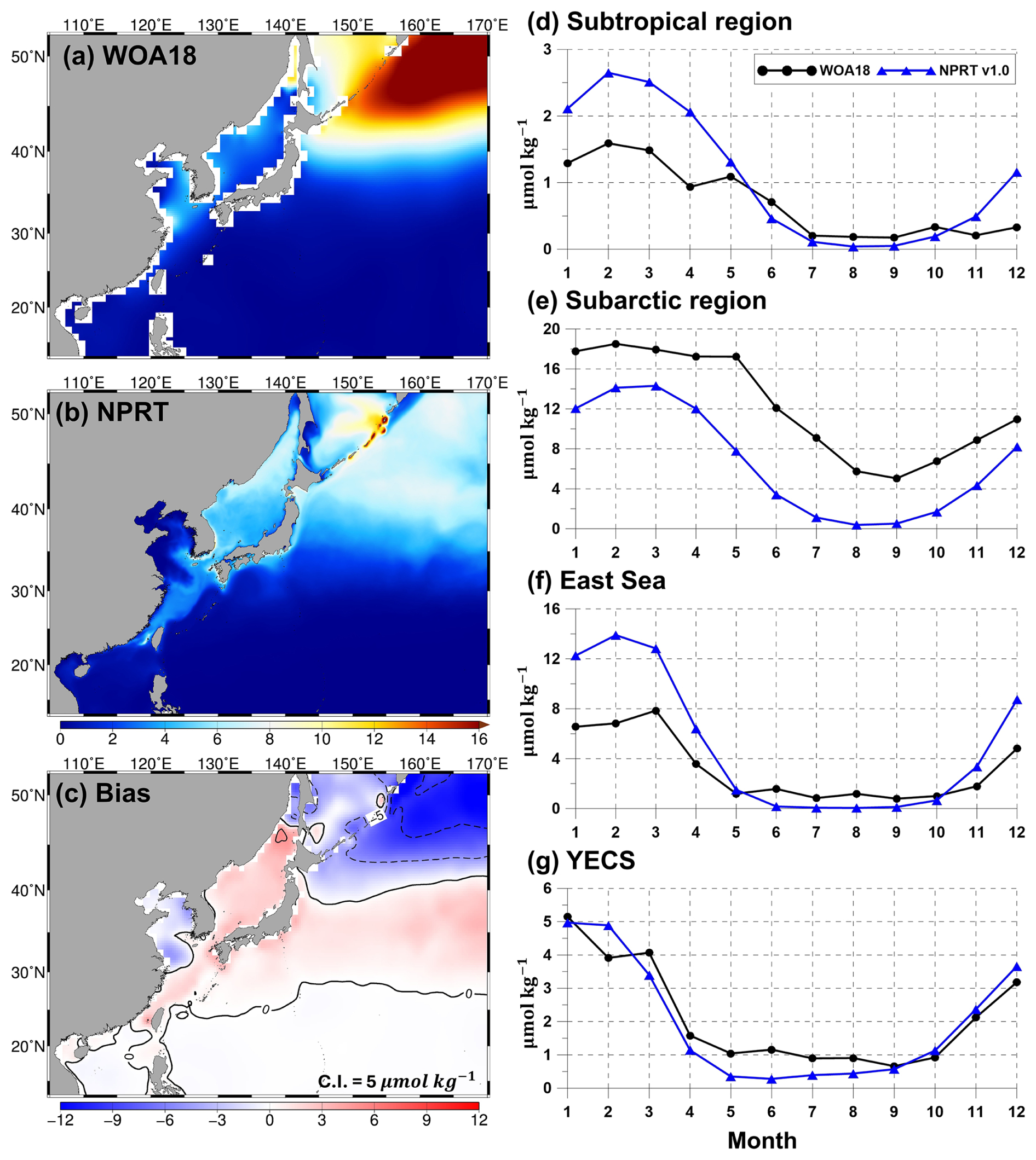
Figure 7 Horizontal distributions of the annual mean surface nitrate concentrations (µmol kg⁻¹) in (a) WOA18, (b) NPRT, and (c) biases between NPRT and observations (WOA18). Seasonal variations in (d) the subtropical region (south of 40° N in the Northwest Pacific), (e) the subarctic region (north of 40° N in the Northwest Pacific), (f) the East Sea, and (g) the Yellow and East China Seas (YECS).

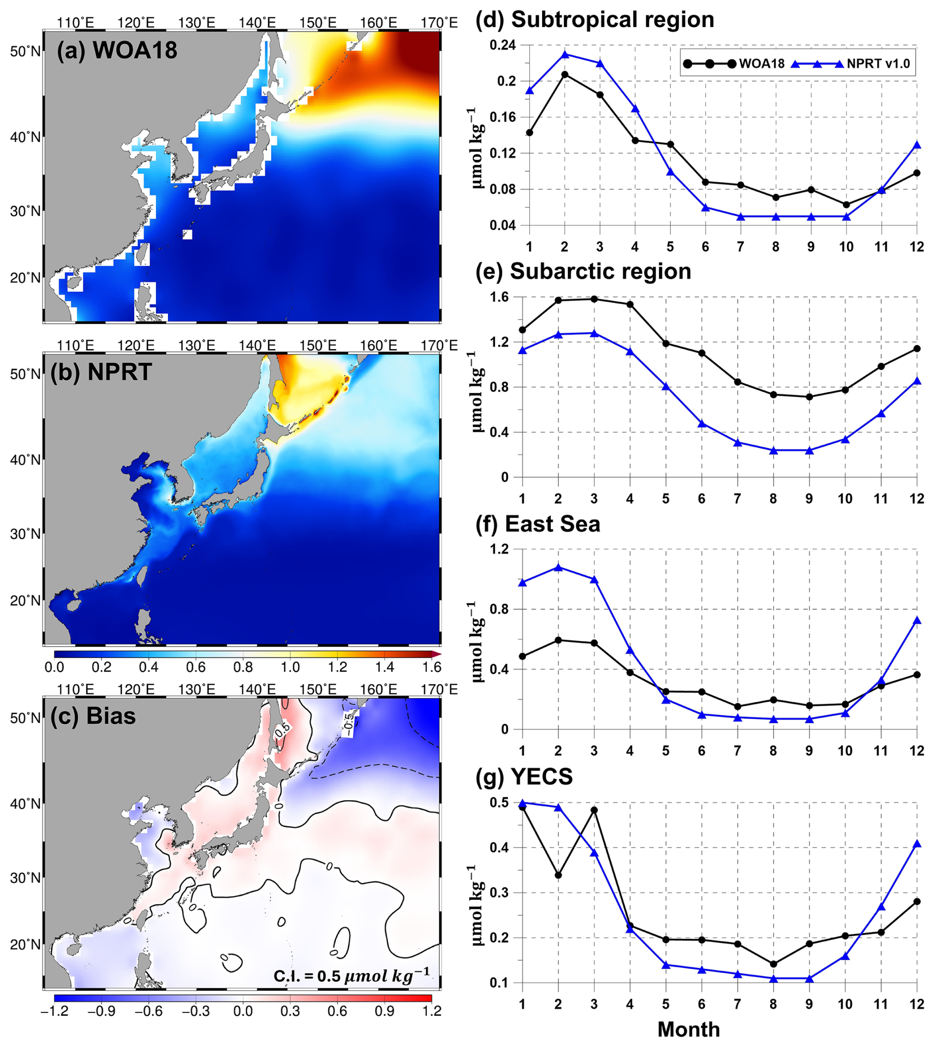
Figure 8 Same as Fig. 7 but applied to the annual mean surface phosphate concentration (µmol kg⁻¹).

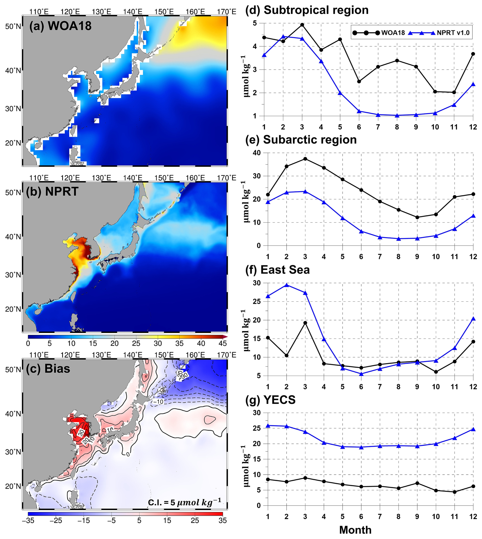
Figure 9 Same as Fig. 7 but applied to the annual mean surface silicate concentration (µmol kg⁻¹).

3.2 Biogeochemistry

3.2.1 Nutrients

The results of the simulated nitrates, phosphates, and silicates, which are essential for the growth of phytoplankton, were compared with the results of the observationally based WOA18 climatology (Figs. 7–9). Figure 7a–c show the comparison of the simulated surface annual mean nitrates with the observed ones. The distribution of the annual mean surface nitrate concentration in the observational data reveals a characteristic increase from low to high latitudes, with concentrations exceeding 15 µmol kg⁻¹ in the subarctic region (Fig. 7a). In the model results, the annual mean concentration of nitrate also increases with increasing latitude and is predominantly distributed in the East Sea, Okhotsk Sea, and the Oyashio extension region (Fig. 7b). Compared with that in the observations, the overall distribution of annual mean surface nitrate concentrations is underestimated (Fig. 7c). In particular, in the subarctic region, the model results exhibit a large negative bias of over −10 µmol kg⁻¹, whereas in the East Sea and the Kuroshio and its extension regions, it exhibits a positive bias. The pattern correlation and RMSE for nitrate in the study area are 0.83 and 5.70 µmol kg⁻¹, respectively. The distribution of the annual mean surface phosphates in NPRT is similar to that in WOA18 (pattern correlation: 0.83; Fig. 8a and b). However, there is a negative bias in the subarctic region and a positive bias in the eastern coast of Sakhalin and the East Sea (Fig. 8c). The bias range is approximately −1.2 to 0.5, and the RMSE is approximately 0.53 µmol kg⁻¹. Unlike other nutrients, the simulated silicate exhibits a significant positive bias (> 30 µmol kg⁻¹) and a negative bias (> 30 µmol kg⁻¹) in the YECS and the subarctic region, respectively (Fig. 9c).

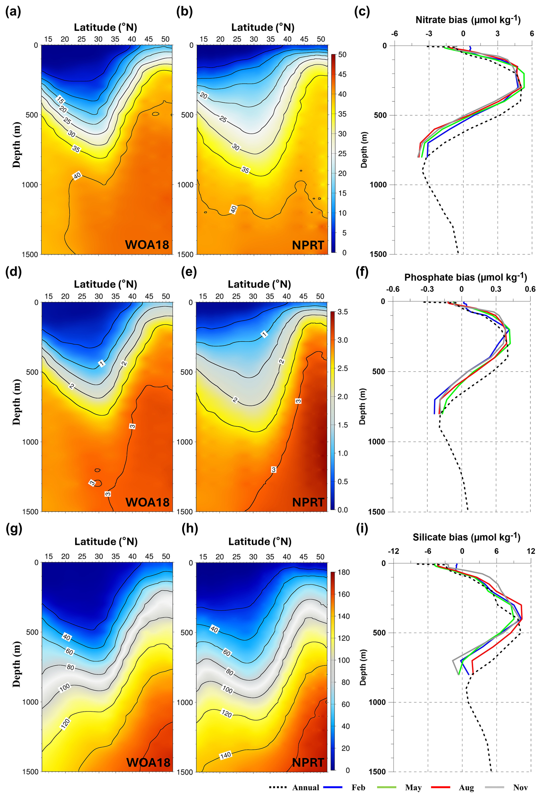
Figure 10 Vertical structures of the zonal averaged annual mean for (a, b) nitrate, (d, e) phosphate, and (g, h) silicate concentrations (µmol kg⁻¹) in the Northwest Pacific. The vertical profile of annual and monthly biases between observation and NPRT results for (c) nitrate, (f) phosphate, and (i) silicate.

The vertical errors of the zonally averaged annual mean nutrients (nitrate, phosphate, and silicate) in the NWP were overestimated south of the Kuroshio–Oyashio Confluence Region (40° N) until a depth of 500 m (Fig. 10). However, in the 500–1500 m, an underestimation error appears which seems to be related to the NPIW simulation. In the intermediate layer of the NWP, the subarctic intermediate water nutrient pool (SINP), with high nutrient concentrations, appears along with the NPIW formed in the Kuroshio–Oyashio Confluence Region (Nishioka et al., 2020, 2021). However, it is considered that the SINP is not distinct in NPRT due to the negative bias in the subarctic region, which is the source of the SINP. Positive biases for nutrients were distributed within a depth of 500 m in all seasons, similar to the annual mean bias, whereas negative biases were exhibited in deeper depths (black solid line in Fig. 10c, f, and i). Regardless of the season, the depth of the positive bias peak for all nutrients is approximately 100–300 m.

The simulated surface nutrient concentrations in NPRT exhibited a clear seasonal variability (Figs. 7–9). In winter, high nitrate concentrations distributed in the subsurface are supplied to the surface by vertical mixing, resulting in an increase in the upper–layer nutrient concentrations from winter to spring. In summer and autumn, distinct seasonal variability is observed, with concentrations gradually decreasing owing to enhanced stratification. The temporal correlation coefficients between the model results and observations (WOA18) for nutrients (nitrate, phosphate, and silicate) are approximately 0.78–0.98, indicating that the seasonal variability is well represented, except for the silicate concentration in the YECS (temporal correlation coefficient: 0.47). In the subarctic region, all nutrients are consistently underestimated regardless of the season, which is likely attributed to the initial and boundary biogeochemical conditions. The initial conditions for nutrients derived from the MOM5–TOPAZ results are approximately 10 µmol kg⁻¹ lower than those derived from the WOA18 data (not shown here).

In addition, we need to give particular attention to the overestimation of silicate in the YECS (Fig. 9). In TOPAZ, silicate is regulated through biogeochemical processes such as dissolution and uptake by large phytoplankton within the mixed layer, as well as by particles sinking into the deep ocean (Dunne et al., 2012). In NPRT, the overestimation of the silicate concentration can be attributed to two possible factors. The first possibility is that silicate, unlike other nutrients, is only considered to be taken up by large phytoplankton. The second factor is that the YECS, which is a shallow marginal sea with a maximum depth of less than 50 m, experiences strong vertical mixing throughout the entire water column due to strong winds, surface heat fluxes during winter, and tidal effects. In shallow marginal seas, rather than a decrease in the upper layer silicate concentration due to particles sinking into the deep ocean, it is speculated that particles remain within the mixed layer, continuously increasing through dissolution. To address the large bias in silicates observed in marginal seas such as the YECS, it is necessary to consider the specific marine environment of each region and adopt accurate parameters and external forcings.

To statistically evaluate the reproducibility of NPRT, this study calculated the monthly Taylor diagram score (TD score; Taylor, 2001; Jin et al., 2023) in each region (Table 1) via the following formulation.

$$\begin{array}{}\text{(3)}& \text{TD (Taylor diagram) score}=\left|\mathrm{1}-R\right|+\left|\mathrm{1}-{\displaystyle \frac{{\mathit{\sigma }}_{\mathrm{M}}}{{\mathit{\sigma }}_{\mathrm{O}}}}\right|+{\displaystyle \frac{E^{\prime }}{{\mathit{\sigma }}_{\mathrm{O}}}},\end{array}$$

where R is the pattern correlation and σ_M and σ_O indicate the standard deviations in the model and observations, respectively. E^′ is the RMSE. The TD scores for nitrate and phosphate concentrations tend to increase from summer to winter, except in the subarctic region. In particular, the TD scores for nitrate in the subtropical region sharply increase in November and December (Table 1), which is due to the large bias distribution in the Kuroshio–Oyashio Confluence Region (not shown here). The positive bias distributed in this region is thought to be due to the relatively high nutrient concentrations in the subsurface in NPRT, which are transported to the surface layer through vertical mixing (Fig. 10). In the subarctic region, the TD scores for all nutrients are greater than 2.5 (Table 1), but as mentioned above, the seasonal variability is well reproduced. Therefore, the dominant negative bias is expected to improve significantly with the use of more accurate initial and boundary conditions. The TD scores for nitrate and phosphate in the East Sea and the YECS are approximately 1.0–2.5 higher than those in the subtropical region. In the case of silicate, the TD score was greater than 10.0 for all months.

3.2.2 N:P ratio

The study area, the Northwestern Pacific, can be broadly divided into three limitation regions: the subtropical and subarctic regions and the YECS, which are characterized by nitrogen limitation (Browning et al., 2022), Fe limitation (Watson, 2001; Zhang et al., 2021), and phosphate limitation (Lee et al., 2023), respectively. The N : P molar ratio in seawater is commonly used to evaluate whether the growth of phytoplankton is potentially limited by nitrogen or phosphorus. Figure 11 shows the distribution pattern of the N : P molar ratio in the Northwestern Pacific. In the subtropical region, the N : P molar ratios in WOA18 and NPRT were approximately 3.4 and 4.3, respectively. However, NPRT shows a clear positive bias in the Kuroshio Current and its extension region. This characteristic is also evident in the distribution of nutrient biases (Fig. 11c). The large meander of the Kuroshio Western Boundary Current significantly influences not only physical characteristics but also biological processes (Hayashida et al., 2023). Therefore, to analyze the biological processes in the Kuroshio meandering region accurately in the future improving the model's representation of Kuroshio meandering is important. In WOA18, the N : P molar ratio in the YECS was approximately 7.3, with the ratio exceeding 16.0, particularly in the Yangtze River estuary, where a distinct phosphate limitation region was observed (Fig. 11a). However, the simulated N : P ratio was relatively lower than the observed values in the Yangtze River estuary (Fig. 11b). As mentioned earlier, despite the significant influence of river discharge in regions such as the YECS, the relatively low N : P molar ratio simulated in this study is likely due to inaccuracies in the estimated nutrient input from riverine sources.

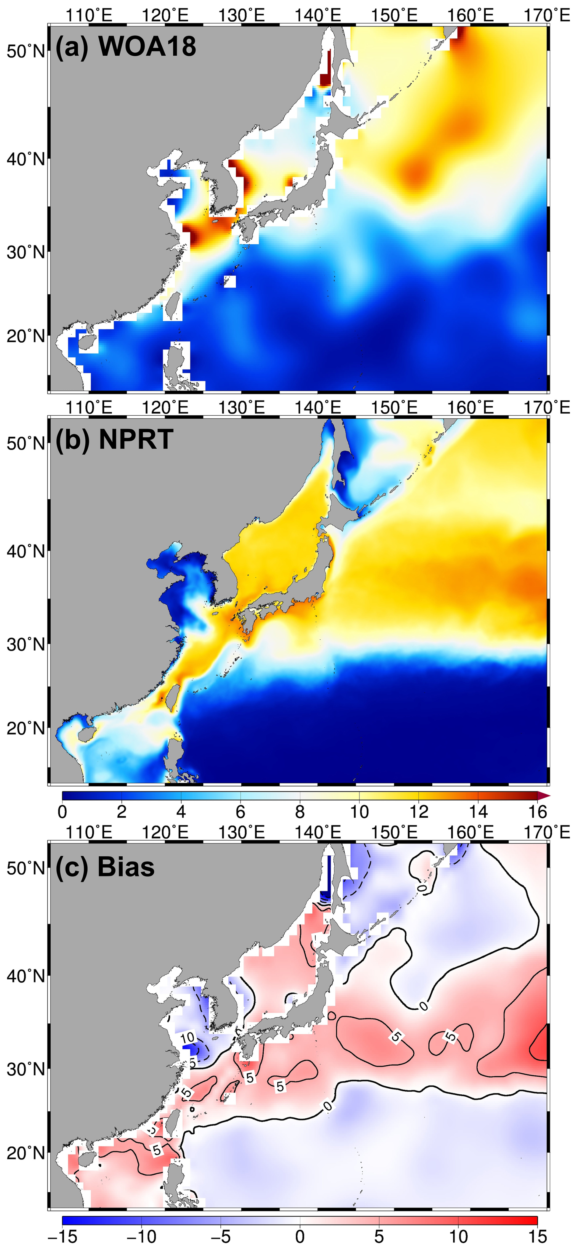
Figure 11 Same as Fig. 3 but applied to the annual mean surface N:P molar ratio.

Table 2 CMIP6 Earth system models used in this study for comparison with chlorophyll concentration.

3.2.3 Chlorophyll

The characteristics of the simulated chlorophyll distributions were compared with those inferred from the MODIS satellite data (Fig. 12). The chlorophyll concentrations derived from satellite data include both sea surface and mixed layer components because of the backscattering effect of reflected light (Jochum et al., 2010; Park et al., 2014; Jung et al., 2020). Therefore, in this study, 0–20 m depth-averaged chlorophyll concentrations from NPRT were compared with satellite data from 2005–2014. Although NPRT was conducted with external forcings that include interannual variations, the results may have several uncertainties due to insufficient spin-up time and/or climatological data for river input and atmospheric deposition. In addition, we analyzed the characteristics of the high-resolution regional model (NPRT) compared with the global biogeochemical models in the CMIP6 datasets. Biogeochemical models include various variables, among which the chlorophyll concentration is influenced by physical factors (temperature and circulation system), light, and various nutrients; these variables exhibit distinct seasonal variability. In this study, we considered the chlorophyll concentration a representative variable for evaluating the performance of biogeochemical models and used a total of ensemble members in the CMIP6 models (Table 2). Among the 13 members (Table 2), ensemble numbers 1 to 8 were calculated using the 0–20 m depth averaged chlorophyll concentration, whereas the remaining ensembles provided only surface data. In addition, we compared the chlorophyll concentrations of GFDL–ESM2M and GFDL–ESM2G (hereafter ESM2M and ESM2G), which are published in the Fifth Assessment Report of Intergovernmental Panel on Climate Change (IPCC AR5), with the NPRT results. Since the historical data for ESM2M and ESM2G are available only up to 2005, we analyzed the data from 1996 to 2005.

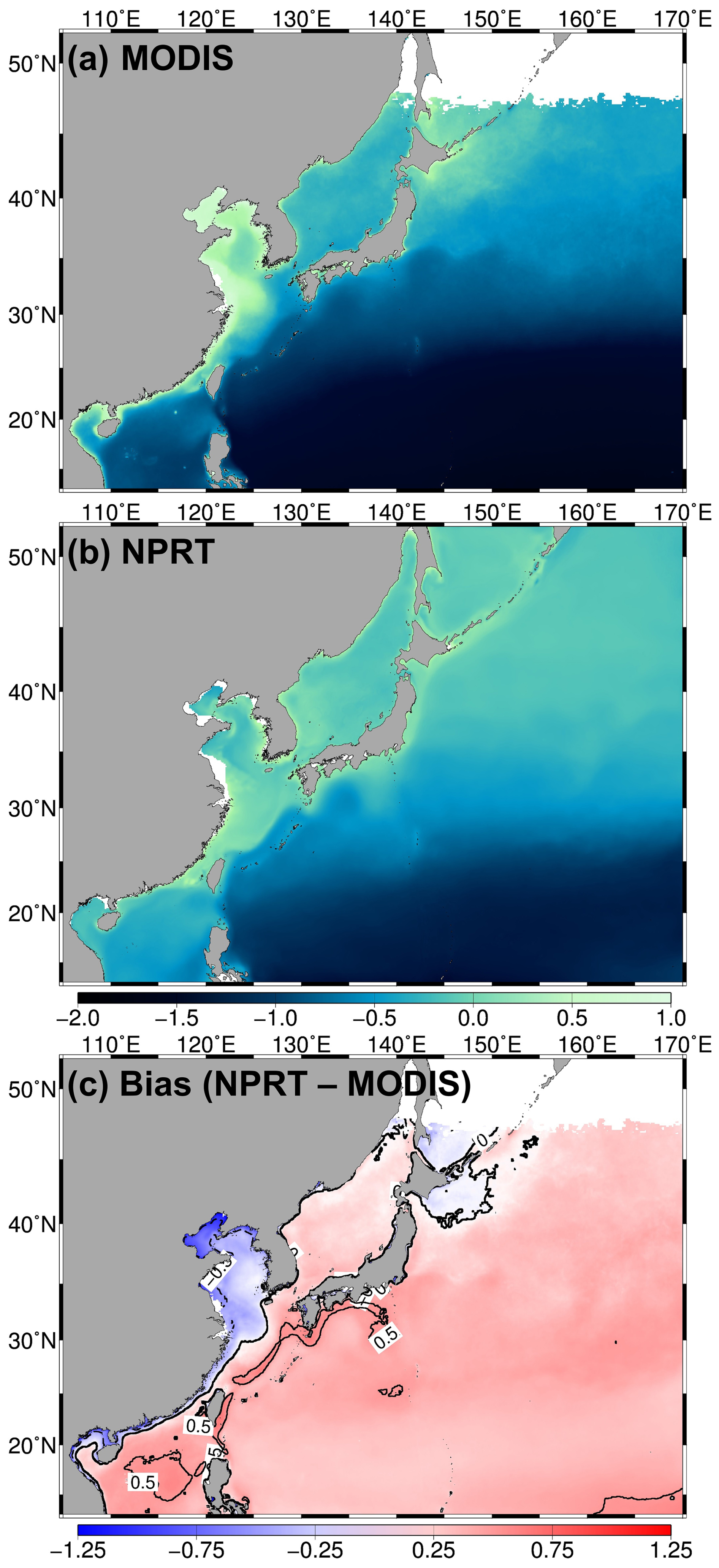
Figure 12 Logarithm of the climatological annual-mean surface chlorophyll concentrations (µmol kg⁻¹) from (a) MODIS, (b) NPRT, (c) bias of between NPRT and observation (MODIS).

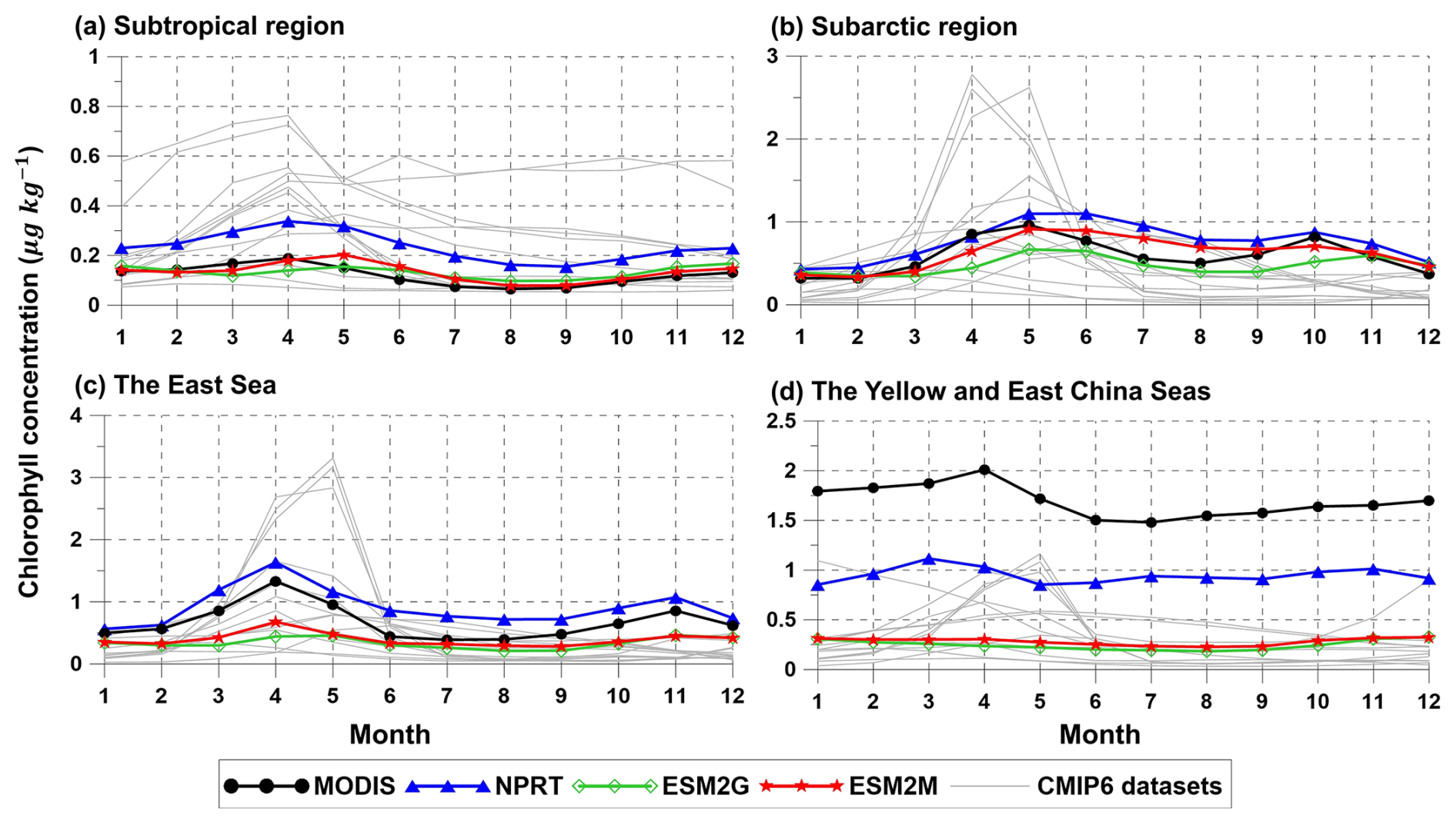
Figure 13 Seasonal variations of the spatial averaged chlorophyll concentrations (µmol kg⁻¹) in (a) the subtropical and (b) subarctic regions, (c) the East Sea, and (d) the YECS. Black, blue, green, red, and light gray lines indicate MODIS, NPRT, GFDL–ESM2G, GFDL–ESM2M, and each ensemble model in CMIP6, respectively.

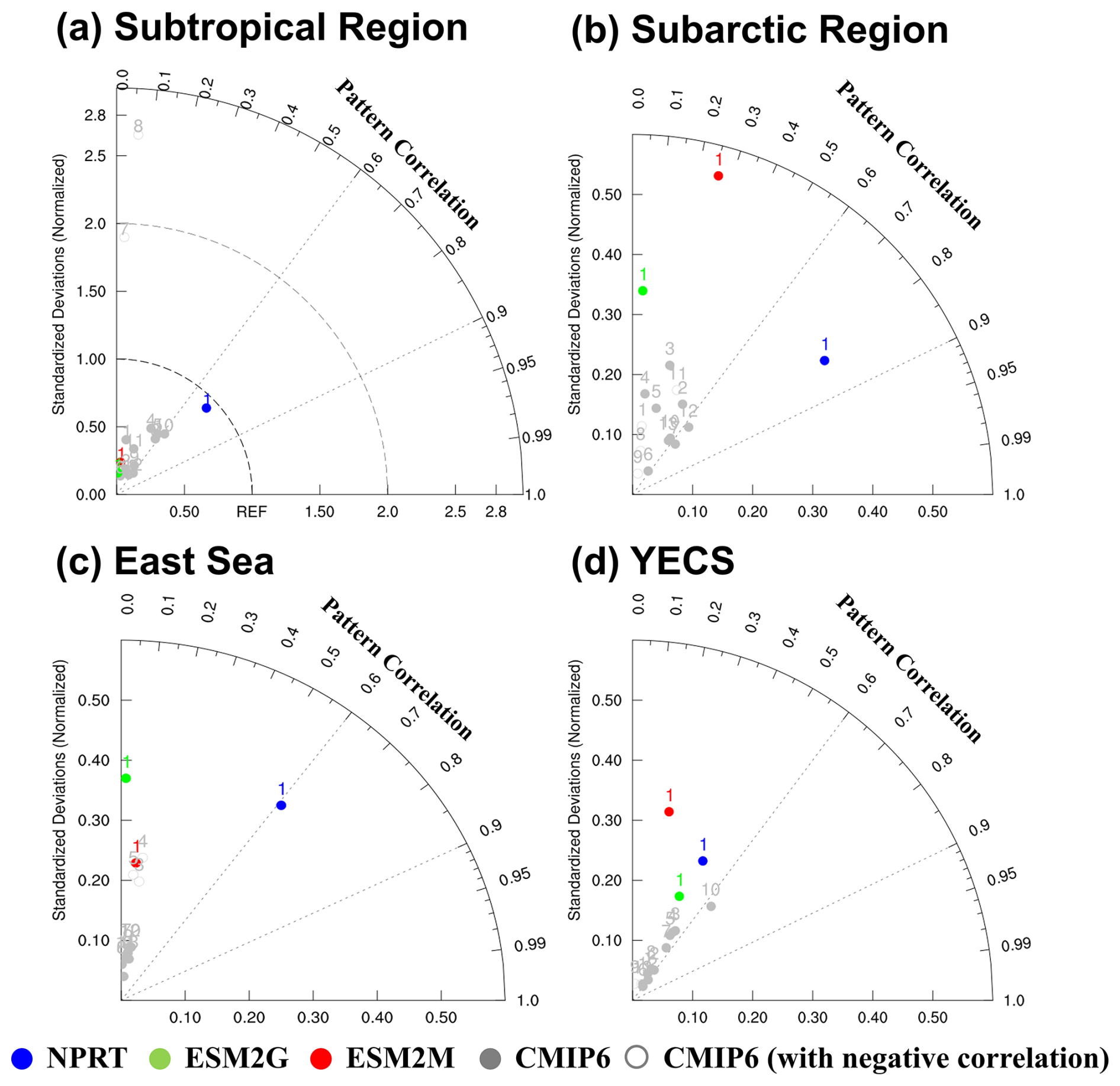
Figure 14 Taylor diagrams (Taylor, 2001) of spatial models (NPRT (blue dots), GFDL–ESM2G (green dots), GFDL–ESM2M (red dots) and each ensemble model in CMIP6 (gray dots)) for surface chlorophyll concentrations compared to observation (MODIS) at each region. The gray open dots (◦) in CMIP6 indicate a negative pattern correlation. Taylor diagrams for time were calculated by comparing observational data with annual mean simulated fields of four models (NPRT, GFDL–ESM2G, GFDL–ESM2M and each ensemble in CMIP6) in the (a) subtropical and (b) subarctic regions, (c) East Sea, and (d) YECS; the numbers represent each ensemble model in Table 1.

Table 3 Summary of the Taylor diagram scores for annual mean surface chlorophyll concentrations in the subtropical and subarctic regions, East Sea, and the Yellow and East China Sea (YECS) in NPRT, each ensemble model in CMIP6, GFDL–ESM2M and GFDL–ESM2G. The subarctic (subtropical) region is north (south) of 40° N in the NWP.

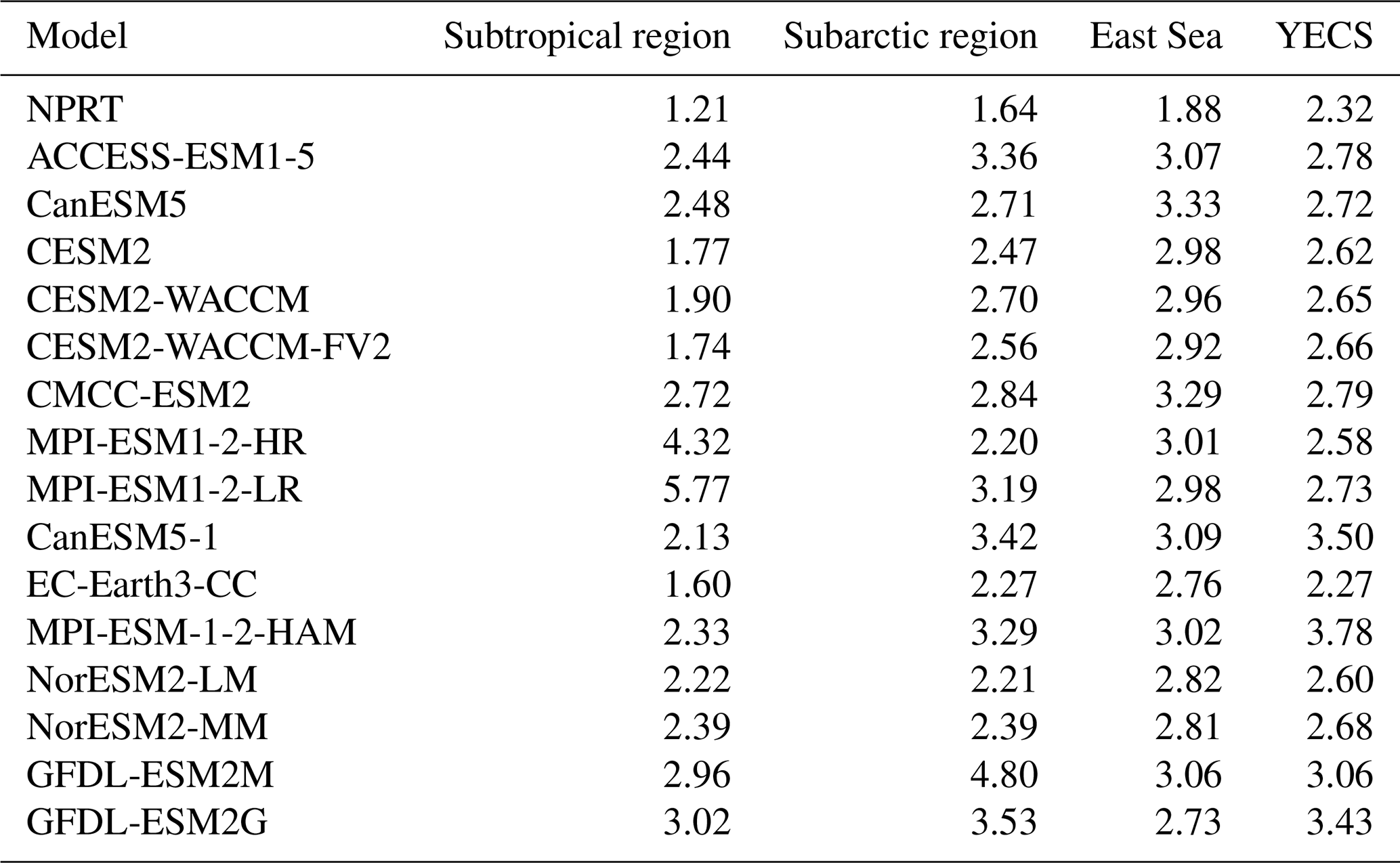
Since the chlorophyll distribution and seasonal variation exhibit different characteristics in each region, the analysis in this study was divided into subtropical and subarctic regions, the East Sea, and the YECS. First, when the data from subtropical and subarctic regions and the East Sea are analyzed, the chlorophyll concentrations generally increase from low to high latitudes according to observations (Fig. 12a). In NPRT, the distribution of the annual mean chlorophyll concentration was similar to the observations in the subtropical region and East Sea (pattern correlations: 0.72 and 0.61, respectively). However, a positive bias is dominant regardless of season, primarily due to the positive bias in nutrients related to phytoplankton growth (Figs. 7–9). Despite the positive biases in the chlorophyll concentration distributions in the subtropical and subarctic regions and the East Sea, as represented in NPRT, the seasonal variation in the chlorophyll concentration, which has spring and autumn biomass peaks, was similar to the observations (Fig. 13a–c). The reproducibility of seasonal variability in NPRT is comparable to the results of ESM2M and ESM2G. However, most of the results of the CMIP6 models do not adequately capture the autumn peak in the subtropical and subarctic regions and East Sea. The pattern correlation ranges of the annual mean chlorophyll concentrations for each ensemble member of CMIP6 in the subtropical and subarctic regions and the East Sea are −0.06 to 0.61, −0.39 to 0.65 and −0.15 to 0.17, respectively (Fig. 14). Some models in the CMIP6 datasets show negative pattern correlations. Although ESM2M and ESM2G were well represented, the range of pattern correlation coefficients was quite low, ranging from −0.12 to 0.26. As a result, the TD scores in NPRT are lower than those in the ESM2M, ESM2G, and CMIP6, especially in the East Sea, and the reproducibility of the chlorophyll concentration distribution has significantly improved (Table 3).

In the YECS, the spatial correlation coefficient in NPRT was approximately 0.45 (Figs. 12a, b and 14d), which was relatively low compared with that in the other regions. However, the NPRT-simulated biomass blooms near the Yangtze River and along the Chinese coast were driven by high freshwater discharge (Fig. 12b). In addition, NPRT, ESM2M and ESM2G effectively reproduced the seasonal variability (spring peak and increasing from summer) that was not captured by the CMIP6 models. In the case of the CMIP6 models, negative bias is dominant regardless of the season (Fig. 13d) and they also lack clear seasonal variability in the chlorophyll concentration. In the YECS, the discharge of freshwater and nutrient concentrations from rivers is one of the most important input forcings determining the spatiotemporal pattern and variability (Zhou et al., 2008). In this study, to apply observation data for freshwater discharge and nutrient concentrations from river outflows, tracer concentrations were determined with a volume flux at the river source point, following an approach similar to that adopted in regional biogeochemical models such as FENNEL (Fennel et al., 2006) and a modified version of the Carbon, Ocean, Biogeochemistry and Lower Trophic model (COBALT; Hauri et al., 2020). However, the chlorophyll concentrations in NPRT still tend to be underestimated (RMSE: 1.62 µmol kg⁻¹) in the YECS, including the Yangtze River estuary (Fig. 12c). Nonetheless, the TD score in NPRT was approximately 2.32, which is lower than that in ESM2M, ESM2G, and CMIP6 (2.23–3.5) (Table 3), and NPRT reproduced the seasonal variability (Fig. 13d) and spatial characteristics such as biomass blooms near the Yangtze River and along the Chinese coast which are driven by high freshwater discharge (Fig. 12b).

In the YECS, the underestimated chlorophyll concentration in NPRT may also be related to the distribution of low nutrient concentrations in the YECS. Furthermore, this can be attributed to the incomplete consideration of the influences exerted by numerous rivers along the Chinese and Korean coasts, as well as the utilization of default data provided by MOM GitHub, which deviates from the actual diverse biogeochemical variables (LITH, NH₄, NO₃, and Fed) introduced from the atmosphere. In addition, we need to consider the uncertainties associated with the satellite observational data from MODIS. MODIS indirectly estimates chlorophyll concentrations by measuring the spectrum of light reflected from the sea surface (visible and near-infrared); however, completely eliminating the influence of colored dissolved organic matter (CDOM) and suspended particles in the water is difficult. Coastal regions, classified as type II waters, are particularly prone to bias in estimated surface chlorophyll concentrations because of the high concentrations of CDOM and suspended particles (Mauri et al., 2007). The CDOM calculated using MODIS data was significantly greater in the YECS than in the other regions (Fig. S2), and the absorption of blue light by CDOM can lead to an overestimation of the chlorophyll concentration (Figs. 12 and S2). In other words, owing to the influence of CDOM, the chlorophyll distribution observed by MODIS may be overestimated, potentially leading to a negative bias in the chlorophyll simulated by NPRT in the YECS. Furthermore, CDOM enhances shortwave heating at the surface while reducing it below the surface (Kim et al., 2016). This process can influence penetrating shortwave radiation, mixing, and surface heat flux. Focusing on the variability in physical processes caused by CDOM could greatly contribute to future research on the interactions between biogeochemistry and physical oceanography.

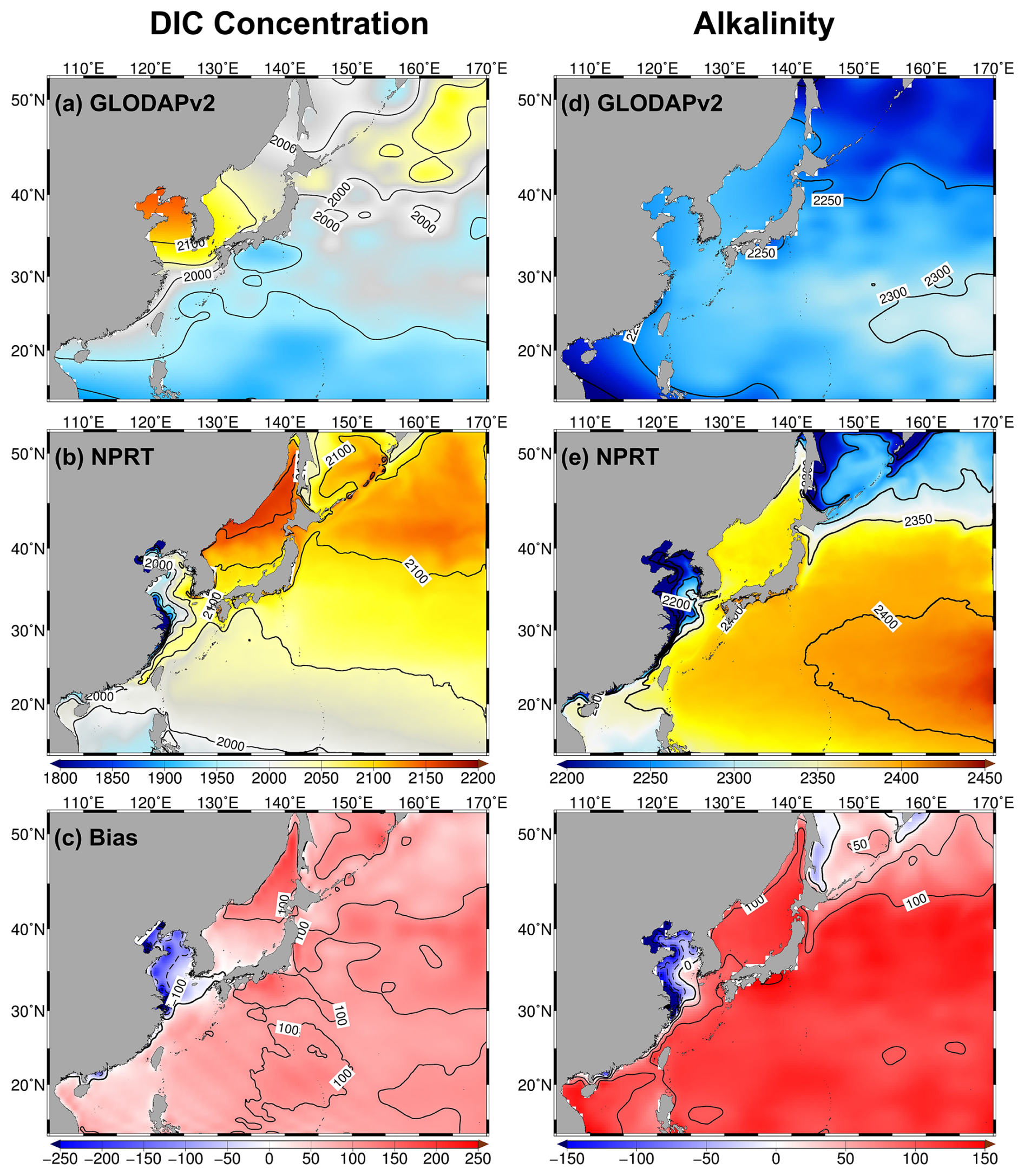
Figure 15 Horizontal distributions of annual mean surface dissolved inorganic carbon (DIC; a–c) concentrations (µmol kg⁻¹) and alkalinity (µeq kg⁻¹; d–f) in the (a, d) GLODAPv2 and (b, e) NPRT in the Northwest Pacific. Biases (c, f) represent NPRT minus observation (GLODAPv2).

3.2.4 Dissolved inorganic carbon and alkalinity

The variables of the carbon system, including dissolved inorganic carbonic (DIC) and alkalinity (Alk), simulated in NPRT were analyzed. First, DIC is a crucial component of ocean biogeochemistry and is directly linked to plankton photosynthesis and respiration; hence, it is a valuable parameter for the analysis of the carbon system (Ding et al., 2018). The results of NPRT, averaged from 2005–2014, were compared with the observed climatological data obtained from GLODAPv2 (Fig. 15a–c). For both the model results and observational data, the annual mean surface DIC concentration in the subarctic region is significantly higher than that in the subtropical region. The simulated annual mean surface DIC concentration in NPRT generally exhibited a positive bias. However, in the YECS, there was a significant negative bias of over −300 µmol kg⁻¹. In particular, low DIC concentrations (below 1900 µmol kg⁻¹) appeared in the Yangtze River estuary. The bias range for the entire study area is approximately between −650 and 180 µmol kg⁻¹, with a pattern correlation of approximately 0.41 and a RMSE of 99.84 µmol kg⁻¹. The GLODAPv2 dataset does not seem to adequately reproduce the low DIC concentrations caused by discharge from the Yangtze River. This is because previous studies using ship-based observations reported that low concentrations are distinctly observed in the Yangtze River estuary (Zhai et al., 2007; Wang et al., 2016). If the YECS are not considered, the pattern correlation and RMSE excluding the YECS are approximately 0.81 and 95.67 µmol kg⁻¹, respectively.

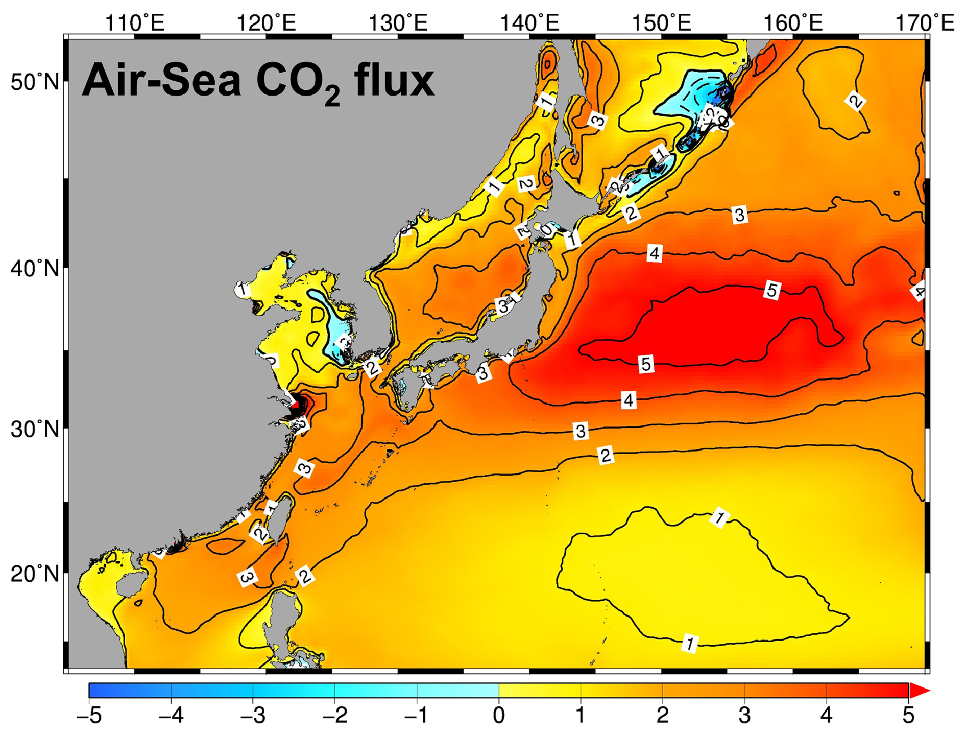
Figure 16 Distribution of the annual mean air–sea CO₂ flux ($\mathrm{mol}{\mathrm{m}}^{-\mathrm{2}}{\mathrm{d}}^{-\mathrm{1}}$) in NPRT in the Northwest Pacific. Positive value indicates the absorption from the atmosphere to the ocean.

The Alk simulated in NPRT also exhibited a significant positive bias (> 150 µeq kg⁻¹) in the study area, excluding the YECS (Fig. 15d–f). The overestimation of Alk in NPRT facilitates the accumulation of pCO₂ from the atmosphere into the ocean, which may contribute to the increase in the surface DIC concentration. The simulated annual mean surface CO₂ flux was predominantly characterized by an influx from the atmosphere to the ocean (Fig. 16). However, it may be premature to conclude that the results of carbonate variables in NPRT are positively biased because the time series of DIC concentrations in MOM5–TOPAZ did not reach the equilibrium state during the spin-up period (Fig. S3). Consequently, the initial and boundary conditions derived from the MOM5–TOPAZ model results exhibit significantly higher DIC concentrations and Alk values than the observations do. In particular, the DIC concentration at the eastern boundary is higher than that observed, which may contribute to the elevated DIC levels in the subtropical region due to the influence of the North Equatorial Current and Kuroshio Current. To improve this bias, more accurate boundary conditions must be considered.

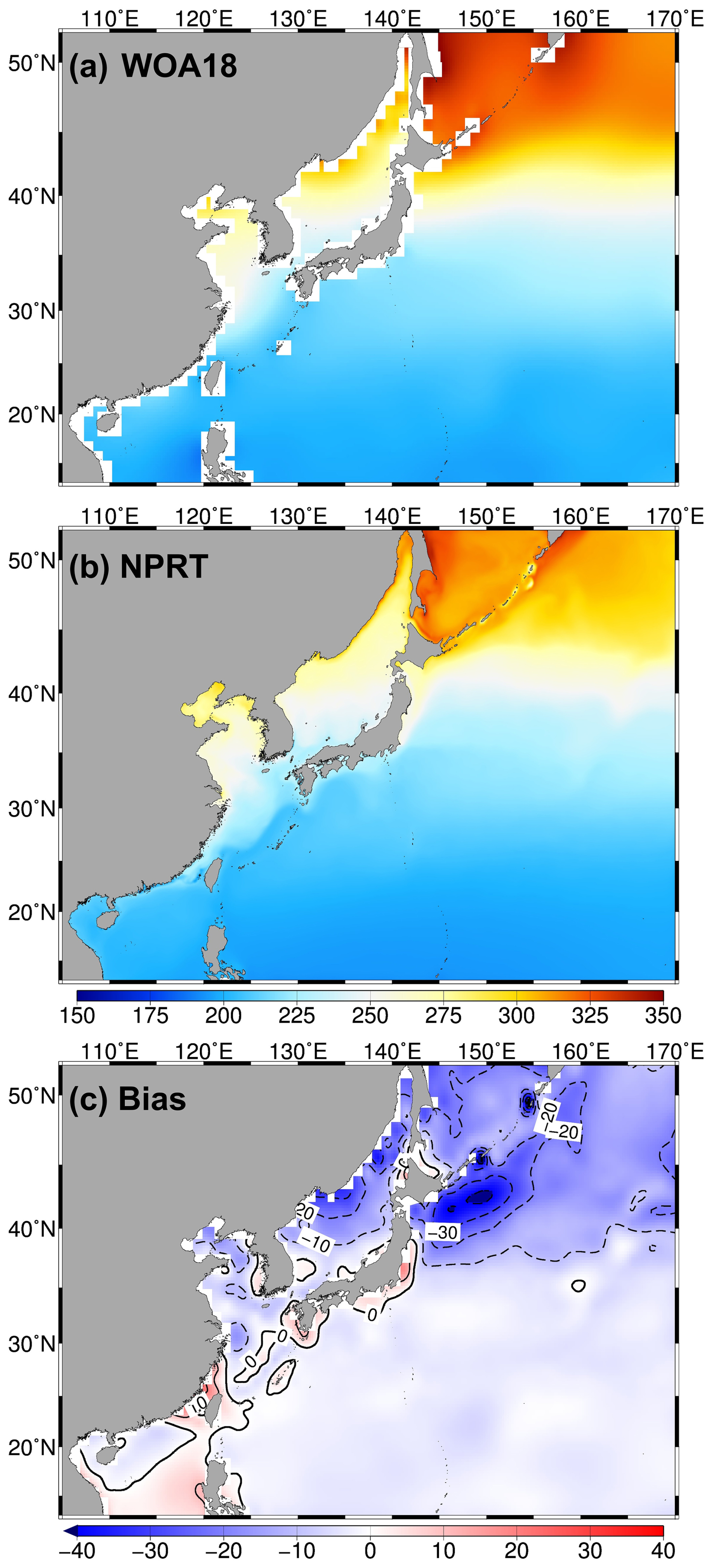
Figure 17 Horizontal distributions of the annual mean surface dissolved oxygen (DO) concentration (µmol kg⁻¹) in (a) WOA18 and (b) NPRT, and (c) bias between NPRT and WOA18.

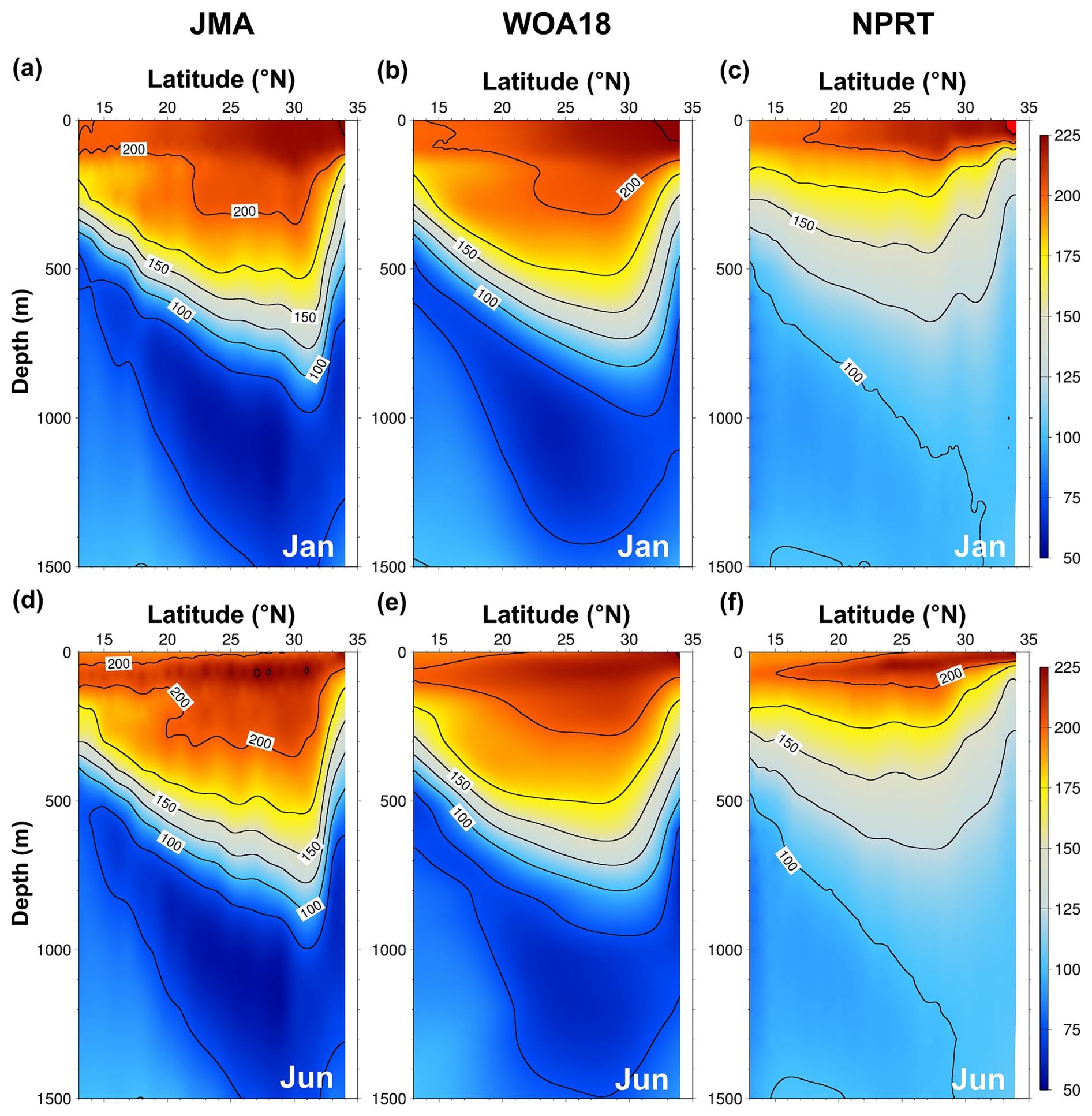
Figure 18 Vertical structures of the annual mean dissolved oxygen (DO) concentration (µmol kg⁻¹) along 137° E line from (a, d) JMA and (b, e) WOA18, and (c, f) NPRT in January (top) and June (bottom).

3.2.5 Dissolved Oxygen

DO is important for analyzing the ecological and physical characteristics of marine ecosystems and serves as a tracer. It is associated with ocean temperature, air–sea exchange, and phytoplankton photosynthesis. The simulated DO results were compared with the WOA18 climatological data and observations from the JMA (Figs. 17 and 18). Both the observations (i.e., WOA18) and the model results demonstrate a typical increase in surface DO concentrations from low to high latitudes, with high concentrations of DO more than 300 µmol kg⁻¹ being distributed in the Okhotsk Sea and the Oyashio region (Fig. 17). With respect to that of the WOA18 observations, the model tends to underestimate DO exhibiting a dominant negative bias (up to approximately −30 µmol kg⁻¹) in the Oyashio region. The pattern correlation and the RMSE of DO concentration between the model results and WOA18 data are 0.99 and 9.99 µmol kg⁻¹, respectively. The primary cause of the negative bias in the simulated DO is related to the positive bias in surface temperature (Figs. 4c and 17c), which is thought to be due to the weakening of thermal solubility. To compare the vertical structures of DO, ship measured DO data from the JMA were employed along the 137° E line across the Kuroshio main path in January and June (Fig. 18). Both the observations and the model results show the presence of an oxycline layer, where the DO decreases sharply with depth. Below this layer, a DO minimum zone is evident. The depth of the DO minimum zone in NPRT appears below 500 m regardless of the season, similar to the observations (JMA); however, the minimum DO concentrations are approximately 25 µmol kg⁻¹ higher than the JMA data. This is presumed to be caused by the weak NPIW formation. These characteristics are also evident in the results obtained using the TOPAZ module (Lee et al., 2022). Consequently, NPRT adequately qualitatively reproduces the spatiotemporal distribution of the DO circulation system. However, sufficient observational data, accurate initial and boundary conditions, improvement in physical processes simulation, and adequate spin-up times are required for quantitative and reproducibility improvements, particularly in the intermediate layer.

4 Conclusions

The coupled physical–biogeochemical ocean model developed in this study, namely ROMS–TOPAZ (NPRT v1.0), is a preliminary investigation that reflects the characteristics of local regions with high resolution, enabling analysis of the interactions between the physical and biogeochemical processes in the ocean. The study area comprises the NWP, East Sea, and YECS, which exhibit diverse characteristics depending on the region. The study area is one of the main regions where nutrients are consumed by primary production. CO₂ exchange between the air and sea is dominant in the NWP (Takahashi et al., 2009; Ishizu et al., 2021); however, in the YECS, the biogeochemical environment is significantly influenced by riverine discharge (Zhou et al., 2008). In these oceanic regions with such diverse features, we evaluated the reproducibility of the spatial distribution and seasonal variability of the physical and biogeochemical variables derived using NPRT. To generate the initial and boundary data for the biogeochemical variables required to simulate NPRT, first MOM5–TOPAZ was integrated for 100 years under the pCO₂ environment and ERA5 was integrated for 2000, after which the model was run for an additional 15 years under actual atmospheric CO₂ concentration conditions (2000–2014). Using the biogeochemical variables reproduced by MOM5–TOPAZ and the physical variables from HYCOM, NPRT was subsequently integrated for 15 years (2000–2014). In this study, model results from the last 10 years (2005–2014) were used in the analysis.

NPRT successfully reproduced the overall spatial distributions, such as upper-layer circulation, the NPIW formation via ventilation, and salinity in the YECS influenced by freshwater input, as well as the seasonal variability in biogeochemical variables. For nutrients (nitrate, phosphates, and silicate), there was a high pattern correlation coefficient for the annual mean surface nutrient concentrations. In particular, both pattern correlation coefficients for nitrate and phosphate concentrations in the study area were approximately 0.83 but the coefficient for silicate was low (approximately 0.42). All nutrients were underestimated in the subarctic region regardless of season, likely because low values were prescribed for the initial and boundary conditions. In contrast, the Kuroshio–Oyashio Confluence Region, characterized by strong vertical mixing, exhibited a positive bias, especially during winter, due to the relatively high nutrient concentrations at the subsurface in NPRT. Although biases are distributed depending on the region, the overall seasonal variability in all nutrients was well simulated. The temporal correlation coefficients for nutrients were approximately 0.78–0.98 in the study area, except for the silicate content in the YECS. In marginal seas at shallow depths, such as the YECS, silicate is presumed to accumulate continuously because of insufficient reduction caused by phytoplankton uptake and particles sinking into the deep ocean due to strong vertical mixing, leading to a significant positive bias. In other words, parameter adjustments considering physical and biogeochemical environments are necessary.

For chlorophyll concentration, although NPRT showed positive and negative biases in the study area, it effectively reproduced not only the seasonal variation in the subtropical and subarctic regions, East Sea, and YCES, but also the improved TD scores in all regions compared with the ESM2M, ESM2G, and CMIP6 data. In addition, in the YECS, because a significant amount of nutrients is discharged from the Yangtze River along with a large amount of freshwater (leading to biomass blooms around the Yangtze River estuary) the chlorophyll concentrations start to increase in July. As a result, low DIC concentrations associated with river effects were also simulated around the Yangtze River. These regional characteristics are difficult to reproduce via low-resolution global models. Furthermore, in the subtropical and subarctic regions, significant positive biases for DIC and Alk were predominantly simulated, which is due to the spin-up time (100 years) in this study being insufficient for reaching the equilibrium state.

In summary, the coupled model NPRT developed in this study is an important tool for studying the interactions between ocean physics and biogeochemistry at a high resolution, enabling research at the regional scale. In the future, this tool is expected to provide a basis for understanding the mechanisms of oceanic physics and biogeochemical environments in various regions, ultimately improving the accurate assessment and predictability of carbon cycling.