Process-based modeling framework for sustainable irrigation management at the regional scale: integrating rice production, water use, and greenhouse gas emissions

Rice cultivation faces multiple challenges from rising food demand as well as increasing water scarcity and greenhouse gas emissions, intensifying the tension of the food–water–climate nexus. Process-based modeling is pivotal for developing effective measures to balance these challenges. However, current models struggle to simulate their complex relationships under different water management schemes, primarily due to inadequate representation of critical physiological effects and a lack of efficient spatially explicit modeling strategies. Here, we propose an advancing framework that addresses these problems by integrating a process-based soil–crop model with vital physiological effects, a novel method for model upscaling, and the non-dominated sorting genetic algorithm II (NSGA-II) multi-objective optimization algorithm at a parallel computing platform. Applying the framework accounted for 52 %, 60 %, 37 %, and 94 % of the experimentally observed variations in rice yield, irrigation water use, methane, and nitrous oxide emissions in response to irrigation schemes. Compared with the original model using traditional parameter upscaling methods, the advancing framework significantly reduced simulation errors by 35 %–85 %. Moreover, it well reproduced the multi-variable synergies and tradeoffs observed in China's rice fields and identified an additional 18 % areas feasible for irrigation optimization, along with an additional 11 % and 14 % reduction potentials of water use and methane emissions, without compromising production. Over 90 % of the potentials could be realized at the cost of 4 % less yield increase and 25 % higher nitrous oxide emissions under multiple objectives. Overall, this study provides a valuable tool for multi-objective optimization of rice irrigation schemes at a large scale. The advancing framework also has implications for other process-based modeling improvement efforts.

1 Introduction

Rice is the staple food for more than half of the world's population and is also the most water-intensive cereal crop with a significant contribution to greenhouse gas emissions (GHGs) (Lampayan et al., 2015; Carlson et al., 2017). Rice cultivation currently accounts for 40 % of global irrigation water use (IRR), 30 % of methane (CH₄), and 11 % of nitrous oxide (N₂O) emissions in agriculture (Yuan et al., 2021). To meet the demand of the growing population, a 50 %–60 % increase in global rice production along with a 15 % increase in water use is required by 2050, potentially leading to higher greenhouse gas emissions and intensifying the food–water–climate tensions of rice fields (Flörke et al., 2018; World Bank, 2017). Therefore, ensuring food security while conserving water resources and reducing GHGs in rice cultivation is essential for achieving multiple United Nations Sustainable Development Goals.

Optimizing water management is promising to address the multiple challenges. However, different water management schemes can lead to a wide range of outcomes in rice yield (−16.9 % to 21.9 %), IRR (−68.0 % to −0.3 %), CH₄ (−85.5 % to −0.1 %), and N₂O (0 % to 364 %) across climatic zones, reflecting complex interactions between environmental factors and management strategies (Bo et al., 2022). Process-based models are powerful tools for predicting and managing the complicated interactions in responses to water management, given their strength in simulating crop growth, water dynamics, and soil biogeochemical processes under diverse genotype × environment × management conditions (Tian et al., 2021; Chen et al., 2022; Yan et al., 2024). Despite several relevant studies at site scales, extrapolation of optimized water management schemes from limited sites to the broader rice growing regions is hindered by the diverse climate, soil, crop variety, field management, etc. (Yan et al., 2024; Liang et al., 2021). Region-specific simulations of the food–water–climate nexus are thus urgently needed to identify tailored solutions. Nevertheless, current models face challenges in accurately predicting yield responses to various water management practices and adequately reproducing the spatial heterogeneity of these responses.

Despite extensive experimental research to understand critical physiological effects underlying yield responses, these processes have not been fully represented in models, especially the compensation mechanisms. Compared to continuous flooding, imposing moderate water deficit and then rewatering the field could increase both effective leaf area and net photosynthetic rate upon re-irrigation to enhance photosynthesis for biomass production (Yang and Zhang, 2010). In addition, harvest index could increase due to enhanced remobilization of assimilates and accelerated grain filling rate (Zhang et al., 2008). However, prevailing models (for example, ORYZA, DSSAT, APSIM, and WHCNS) primarily focus on the negative impacts of water deficit (i.e., reduced photosynthesis or leaf rolling), while neglecting or indirectly simulating crop adaptation processes (e.g., enhanced root growth and water uptake in deeper soil layers) (Bouman et al., 2001; Li et al., 2017; Liang et al., 2021; Tsuji et al., 1998). As a consequence, yield sensitivities to water management could be overestimated, as evidenced by evaluations of the ORYZA (v3) model (Xu et al., 2018). Moreover, physiological processes respond differently to water availability at different growth stages, while crop models generally use a constant water effect coefficient throughout the rice growing season (Ishfaq et al., 2020). These imply model deficiencies in predicting yield response to water management, although no assessment across large scales exists.

Accurate model parameters are essential for reproducing spatial heterogeneity of yield, IRR, and GHGs. Previous studies usually used either the same parameters at different pixels, calibrated against all observations, or the spatial proximity principle to extrapolate model parameters for regional simulations, as a result of a lack of sufficient observations (Zhang et al., 2024, 2016). However, critical model parameters varied considerably when calibrated under different environmental and management conditions, reflecting important impacts of these factors on underlying physiological and biogeochemical processes (Tan et al., 2021). As a consequence, traditional model parameterization approaches are unlikely to capture variability of yield, IRR, and GHGs due to their neglect of the environmental and management-related impacts (Song et al., 2023; Zhang et al., 2023). Besides, previous studies only evaluated simplified irrigation protocols (i.e., once drainage at midseason or alternative wetting and drying with a constant threshold across the growing season) or only set bi-objectives as optimization targets (Tian et al., 2021; Chen et al., 2022), which likely underestimated the regulation potentials. Therefore, an integrated framework composed of a reliable modeling platform, broader water management schemes, and multi-objective optimization targets is required for sustainable water management optimization.

To address these challenges, this study proposed an advancing framework that integrated a process-based soil–crop model (Soil Water Heat Carbon Nitrogen Simulator, WHCNS) with key physiological effects, a novel model upscaling method, and a multi-objective optimization algorithm (non-dominated sorting genetic algorithm II, NSGA-II) at a parallel computing platform (see Fig. 1 for workflow). This study focused on rice yield (yield), irrigation water use (IRR), methane (CH₄), and nitrous oxide emissions (N₂O) of irrigated rice fields. First, three physiological effects were quantified and embedded into WHCNS to enhance the prediction of yield responses. Regionalized model parameters were then derived by developing parameter transfer functions for regional simulations. The model's ability to reproduce the variations in the food–water–climate nexus was extensively validated against field observations. Multi-objective optimization was conducted using NSGA-II to investigate tradeoffs within the food–water–climate nexus and assess the regulation potentials of water management optimization. This framework was applied to China's rice cropping system as an example, considering its position as the world's largest rice producer and the ongoing conflicts between production demand, water scarcity, and greenhouse gas emissions. This study aims to provide a valuable framework for predicting and regulating rice's food–water–climate nexus towards sustainable water management.

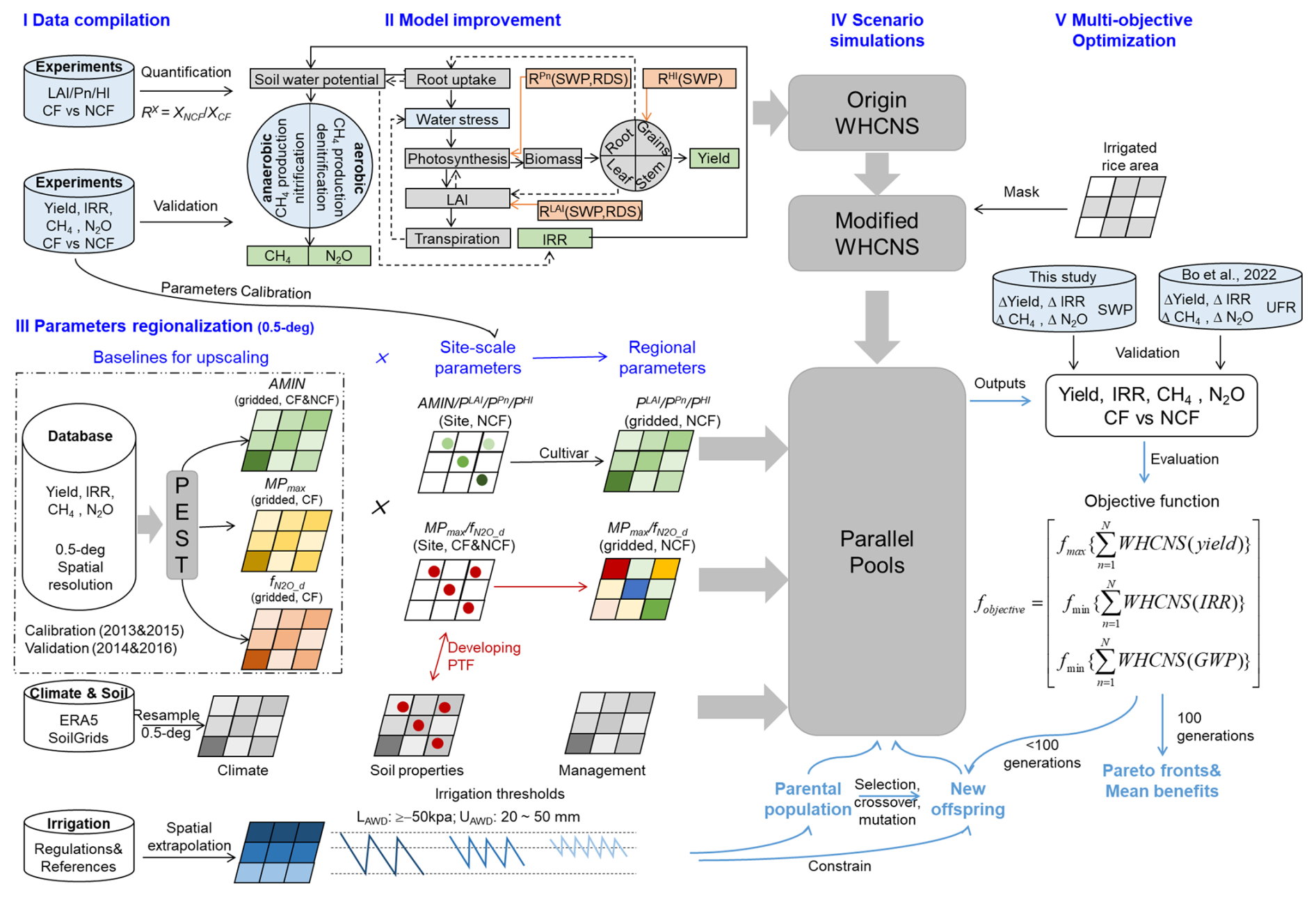
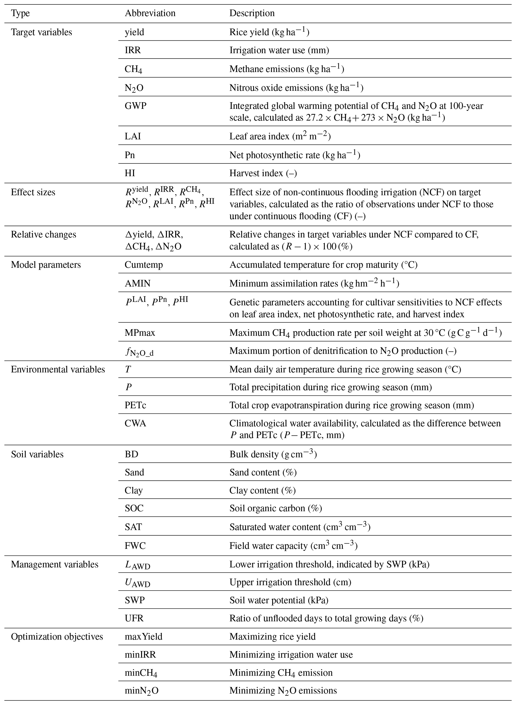
Figure 1 Research framework of this study. The framework mainly combines data compilation, model improvement, parameter regionalization, scenario simulations, and multi-objective optimization. The framework can be flexibly adapted with alternative irrigation scenarios, optimization objectives, and optimization algorithms in other modeling studies. LAI, Pn, and HI represent leaf area index, net photosynthetic rate, and harvest index. AMIN, MPmax, $f_{{\mathrm{N}}_{\mathrm{2}}\mathrm{O}\mathrm{\_}\mathrm{d}},P^{\mathrm{LAI}}$, P^Pn, and P^HI are model parameters calibrated and mapped in this study (Sect. 2.4). CF and NCF represent continuous flooding and non-continuous flooding irrigation. SWP and UFR represent soil water potential and the ratio of unflooded days to total rice growing days, indicating different irrigation schemes. (See Table A1 for detailed descriptions of parameters and variables.)

2 Data and methods

2.1 WHCNS model and input data

The soil Water Heat Carbon Nitrogen Simulator (WHCNS) model was improved and incorporated into the advancing framework in this study to simulate rice yield, irrigation water use (IRR), methane (CH₄), and nitrous oxide (N₂O) emissions of irrigated rice fields at each pixel. The WHCNS model is a process-based agroecosystem model that runs at a daily time step and comprises six major components: surface ponding water dynamics, soil water movements, soil heat transfer, soil N transformation and transport, soil organic turnover, and crop growth. Detailed model descriptions can be found in Liang et al. (2022, 2023, 2021). This model was chosen for several considerations: (i) The model directly outputs all four target variables simultaneously. This avoids biogeochemical models relying on crop models for detailed physiological parameters to simulate yield and calculating IRR externally to obtain all four targets as previously done (Tian et al., 2021; Yan et al., 2024). (ii) The model has been proven to simulate the effects of frequent dry–wet cycles effect reasonably well in Chinese rice fields, due to simulating water and nitrogen dynamics in the surface ponding water layer that is specific to rice fields (Liang et al., 2021). (iii) The model is executable at both site and regional scales with high efficiency and performs well in capturing spatial variation in key processes (Liang et al., 2023). (iv) The model has a very flexible irrigation setup, which allows for the precise control of paddy field water surface levels by setting the minimum and maximum irrigation thresholds. It also enables calculating water usage for paddy field irrigation under various water management scenarios (Jiang et al., 2021). The model is particularly suitable for simulating the regional food–water–climate nexus of rice fields.

This study ran the model at both site and regional scales (0.5 degree spatial resolution). Model input data include daily meteorological variables, soil properties by depth, and management variables related to planting, fertilization, and irrigation (Table S1). For site-scale simulations, these variables were obtained from experimental studies; if unreported, they were extracted from spatial datasets according to geographical locations. All spatial datasets were resampled to 0.5° spatial resolution for regional simulations. (1) Meteorological variables, including daily mean, maximum, and minimum air temperature; wind speed; precipitation; humidity; and downward solar radiation, were obtained from the fifth-generation ECMWF reanalysis (ERA5) at 0.25° resolution (Hersbach et al., 2023). (2) Soil data, including bulk density, clay contents, and soil hydraulic properties (i.e., saturated water content, field water capacity, wilting point, and saturated hydraulic conductivity) at soil depths of 5, 15, 30, 60, 100, and 200 cm, were obtained from SoilGrids (10 km) (Han et al., 2015). (3) The planting and harvest dates were obtained from the crop calendar data of the Global Gridded Crop Model Intercomparison (GGCMI) phase 3 (Jägermeyr et al., 2021). (4) Fertilization practices were conducted by the auto-fertilization component of the WHCNS model, assuming no nitrogen stress (Liang et al., 2023). (5) Irrigation practices are defined by three variables at a daily step, including upper threshold (U_IRR), lower threshold (L_IRR, with a positive value representing field water level and a negative value representing soil water potential at 15 cm below the soil surface), and maximum allowable field water level after rainfall (H_p, also referred to as bund height). Since there is no spatially explicit information about realistic water management schemes, daily irrigation thresholds were set following Chen et al. (2022) for regional simulations. The model simulates field water level of surface ponding layer and soil water potential of stratified layers at a daily step. Irrigation would be triggered whenever field water level (L_IRR > 0) or soil water potential at 15 cm below the soil surface (L_IRR < 0) reaches the predetermined L_IRR. Irrigation demand is then calculated as the differences between L_IRR and U_IRR.

2.2 Compilation of experimental observations

Extensive literature reviews were conducted to collect experimental observations for model improvement and parameter calibration. Relevant studies should meet the following criteria: (1) Only field experiments covering an entire growing season were included, while pot and laboratory experiments under controlled environmental conditions were excluded. (2) The control and treatments only differed with respect to water management, with continuous flooding (CF) as the control and non-continuous flooding irrigation (NCF) as the treatment but not with respect to other agronomic practices (e.g., cropping intensity, fertilizer management, and tillage). This was to isolate water management effects while avoiding confounding effects of other factors. (3) Upper and lower irrigation thresholds were explicitly reported, and lower thresholds were indicated by soil water potential measured at the soil depth of 15–20 cm. Observations based on soil water potential at other soil depths or other soil-water indicators (e.g., soil water contents) were excluded. (4) At least one of the target variables was observed, including rice yield (yield), irrigation water use (IRR), methane emissions (CH₄), nitrous oxide emissions (N₂O), leaf area index (LAI), net photosynthetic rate (Pn), and harvest index (HI). For LAI and Pn, the growth stages of observations (i.e., tillering, booting, heading, and ripening stage) were recorded to account for growth stage-dependent effects. As a result, we collected observations of 119 experiments from 37 studies covering 28 sites in six countries (i.e., China, India, Philippines, Japan, Bangladesh, and Peru) (Fig. S1). These observations were split into two datasets according to target variables. The first dataset including yield, IRR, CH₄, or N₂O observations was used for calibration of model parameters. The second dataset of LAI, Pn, or HI observations was used to quantify water management effects on physiological processes for model improvement (Sect. 2.3).

For each paired observation under the control and treatment, the effects of non-continuous flooding irrigation were calculated as the ratio of observations under treatment to those under control (Eq. 1). This yielded 251 records for R^yield, 235 for R^IRR, 37 for $R^{{\mathrm{CH}}_{\mathrm{4}}}$,14 for $R^{{\mathrm{N}}_{\mathrm{2}}\mathrm{O}}$, 561 for R^LAI (including 61 from tillering stage, 159 from booting stage, 202 from heading stage, and 139 from ripening stage), 84 for R^Pn (including 42 between the tillering and filling stages), and 351 for R^HI, calculated as follows:

$$\begin{array}{}\text{(1)}& R^X=X_{{}^{\mathrm{NCF}}}/X_{{}^{\mathrm{CF}}},\end{array}$$

where R^X represents non-continuous flooding effects (NCF) on target variables X (including yield, IRR, CH₄, N₂O, LAI, Pn, and HI), and X_NCF and X_CF represent variable values under non-continuous flooding (NCF) and continuous-flooding irrigation (CF), respectively. Relative changes in target variables were calculated as (R^X−1) × 100 for interpretation and representation (e.g., Δyield, ΔIRR, ΔCH₄, ΔN₂O).

For each paired observation, four categories of information were also collected. First, climatic variables included mean daily air temperature (T), precipitation (P), and crop evapotranspiration (ETc) during the growing season. The difference between P and ETc was further calculated to indicate climatological water availability (CWA). Second, soil variables included sand content, bulk density (BD), soil organic carbon (SOC), pH, and soil hydrological properties (e.g., saturated water content (SAT), field water capacity (FWC)). Third, management-related variables included nitrogen application rate, timing, and lower (L_AWD) and upper (U_AWD) irrigation thresholds. Fourth, experimental parameters included geographical location (latitude, longitude), dates of seeding (also transplanting date in transplanted systems), anthesis, and harvest. These variables were used for running WHCNS (Sect. 2.1) and conducting correlation analyses (Sect. 3.1).

2.3 Model improvement

2.3.1 Incorporation of physiological effects

In the original WHCNS model, water management effects on crop growth were simulated by calculating the water stress factor based on the Feddes reduction function (Feddes and Zaradny, 1978). Specifically, the water stress factor is calculated at a daily step as a function of soil water potential to reduce root water uptake, assuming 70 and 1500 kPa as thresholds for when root water uptake starts to decrease and approaches 0 (Eqs. 2–3). The calculated water stress factor was used to reduce the simulated actual biomass production rate, which further indirectly impacted the produced biomass allocated for leaf growth and yield formation, as shown in the following equations (Eqs. 4–6):

$$\begin{array}{}\text{(2)}& {\displaystyle }{T}_{\mathrm{a}}=\underset{L_{\mathrm{R}}}{\int }S(h,h_{\mathrm{\Phi }},z)\mathrm{d}z=T_{\mathrm{p}}\underset{L_{\mathrm{R}}}{\int }{a}_{\mathrm{w}}(h,z)a_{\mathrm{s}}(h_{\mathrm{\Phi }},z)b\left(z\right)\mathrm{d}z,\text{(3)}& {\displaystyle }\mathrm{cf}\left(w\right)={\displaystyle \frac{T_{\mathrm{a}}}{T_{\mathrm{p}}}}=\left\{\begin{array}{l}\frac{\underset{L_{\mathrm{R}}}{\int }{a}_{\mathrm{w}}(h,z)a_{\mathrm{s}}(h_{\mathrm{\Phi }},z)b\left(z\right)\mathrm{d}z}{\mathit{\omega }}=\frac{\mathit{\omega }}{\mathit{\omega }}=\mathrm{1}\mathit{\omega }>{\mathit{\omega }}_{\mathrm{c}}\\ \begin{array}{l}\\ \frac{\underset{L_{\mathrm{R}}}{\int }{a}_{\mathrm{w}}(h,z)a_{\mathrm{s}}(h_{\mathrm{\Phi }},z)b\left(z\right)\mathrm{d}z}{{\mathit{\omega }}_{\mathrm{c}}}=\frac{\mathit{\omega }}{{\mathit{\omega }}_{\mathrm{c}}}<\mathrm{1}\end{array}\mathit{\omega }\le {\mathit{\omega }}_{\mathrm{c}}\end{array},\right.\text{(4)}& {\displaystyle }\begin{array}{rl}& \mathrm{Fgc}=\mathrm{DL}\times {\displaystyle \frac{\mathrm{AMAX}}{K_{\mathrm{e}}}}\\ & \times \ln \left[{\displaystyle \frac{\mathrm{AMAX}+\mathrm{CC}}{\mathrm{AMAX}+\mathrm{CC}\times (-\mathrm{LAI}\times K_{\mathrm{e}})}}\right]\end{array},\text{(5)}& {\displaystyle }\mathrm{Fgass}=\mathrm{Fgc}\times {\displaystyle \frac{\mathrm{30}}{\mathrm{44}}}\times \mathrm{cf}\left(w\right)\times \mathrm{cf}\left(\mathrm{N}\right),\text{(6)}& {\displaystyle }\mathrm{GAA}\left(\mathrm{org}\right)=\mathrm{Fgass}\times \mathrm{fr}\left(\mathrm{org}\right),\end{array}$$

where T_a and T_p are actual and potential root water uptake (cm d⁻¹). L_R indicates root length (cm). a_w(h,z) and a_s(h_Φ,z) are water and salt stress functions. b(z) is the root distribution function. w_c is the critical threshold of volumetric soil water content w above which root water uptake is reduced in water-limited layers of the root zone, but the plant compensates by uptaking more water from other layers that have sufficient available water. Fgc is the daily potential dry matter production accounting for the light interception, radiation use efficiency, and the CO₂ effects (kg hm⁻² d⁻¹). AMAX is the maximum assimilation rate accounting for temperature effect (kg hm⁻² h⁻¹). DL, K_e, and CC indicate day length (h d⁻¹), extinction coefficient (–) and actual radiation use (kg hm⁻² h⁻¹). Fgass is the daily actual dry matter production (kg hm⁻² d⁻¹) accounting for water (cf(w)) and nitrogen stress (cf(N)). GAA indicates the produced biomass allocated to organs (leaf or grains) (kg hm⁻² d⁻¹) with the fraction fr(org).

To modify the WHCNS, NCF effects on leaf expansion, photosynthesis rate, and assimilate partition were quantified based on experimental observations and incorporated into WHCNS (Fig. S2). To do so, mean values of observed effects were first calculated by experimental gradient of soil water potential (SWP, negative values) and rice development stages (RDS, 0–1) (Tables S2–S4). The RDS corresponds to planting, tillering, booting, heading, and filling, and maturity stages were quantified as 0, 0.20, 0.40, 0.55, 0.75, and 1. Effects at other levels of SWP and RDS were then estimated by bilinear interpolation (i.e., F^LAI(SWP, RDS), F^Pn(SWP, RDS), F^HI(SWP)). Three functions were thus developed involving three new genetic parameters to account for differences in cultivar sensitivities (P^LAI, P^Pn, P^HI, Eqs. 7–9). The three functions were added to the original crop growth module to modify simulations of leaf area index, net photosynthesis rate, and biomass allocated into grains (Eqs. 10–12, Fig. 2a).

$$\begin{array}{}\text{(7)}& {\displaystyle }\begin{array}{rl}{R}^{\mathrm{LAI}}(\mathrm{SWP},\mathrm{RDS})& =\mathrm{1}+\left[\left(F^{\mathrm{LAI}}(\mathrm{SWP},\mathrm{RDS})\right)-\mathrm{1}\right]\\ & \times P^{\mathrm{LAI}},\end{array}\text{(8)}& {\displaystyle }{R}^{\mathrm{Pn}}(\mathrm{SWP},\mathrm{RDS})=\mathrm{1}+\left[\left(F^{\mathrm{Pn}}(\mathrm{SWP},\mathrm{RDS})\right)-\mathrm{1}\right]\times P^{\mathrm{Pn}},\text{(9)}& {\displaystyle }{R}^{\mathrm{HI}}\left(\mathrm{SWP}\right)=\mathrm{1}+\left[F^{\mathrm{HI}}\left(\mathrm{SWP}\right)-\mathrm{1}\right]\times P^{\mathrm{HI}},\text{(10)}& {\displaystyle }{\mathrm{LAI}}^{\prime }=\mathrm{GAA}\left(\mathrm{leaf}\right)\times \mathrm{SLA}\times R^{\mathrm{LAI}},\text{(11)}& {\displaystyle }{\mathrm{AMAX}}^{\prime }=\mathrm{AMAX}\times R^{\mathrm{Pn}},\text{(12)}& {\displaystyle }\mathrm{GAA}\left(\mathrm{grains}\right){}^{\prime }=\mathrm{Fgass}\times \mathrm{fr}\left(\mathrm{grains}\right)\times R^{\mathrm{HI}},\end{array}$$

where R^LAI, R^Pn, and R^HI represent NCF effects on leaf area index, net photosynthetic rate, and harvest index, respectively. SWP represents soil water potential at 15–20 cm soil depth. RDS represents relative development stages (0–1). P^LAI, P^Pn, and P^HI are genetic parameters indicating cultivar sensitivities to irrigation regulation that were calibrated based on observations (Sect. 2.4). LAI and SLA are leaf area index (m² m⁻²) and specific leaf area (m² kg⁻¹). LAI', AMAX', and GAA(grains)' denote simulations of the modified model. It is worth noting that the three functions can be flexibly coupled to other process-based crop models to modify the simulation of leaf area growth, biomass production, and allocation processes. The genetic parameters need to be recalibrated against observed yield responses, considering different model structures.

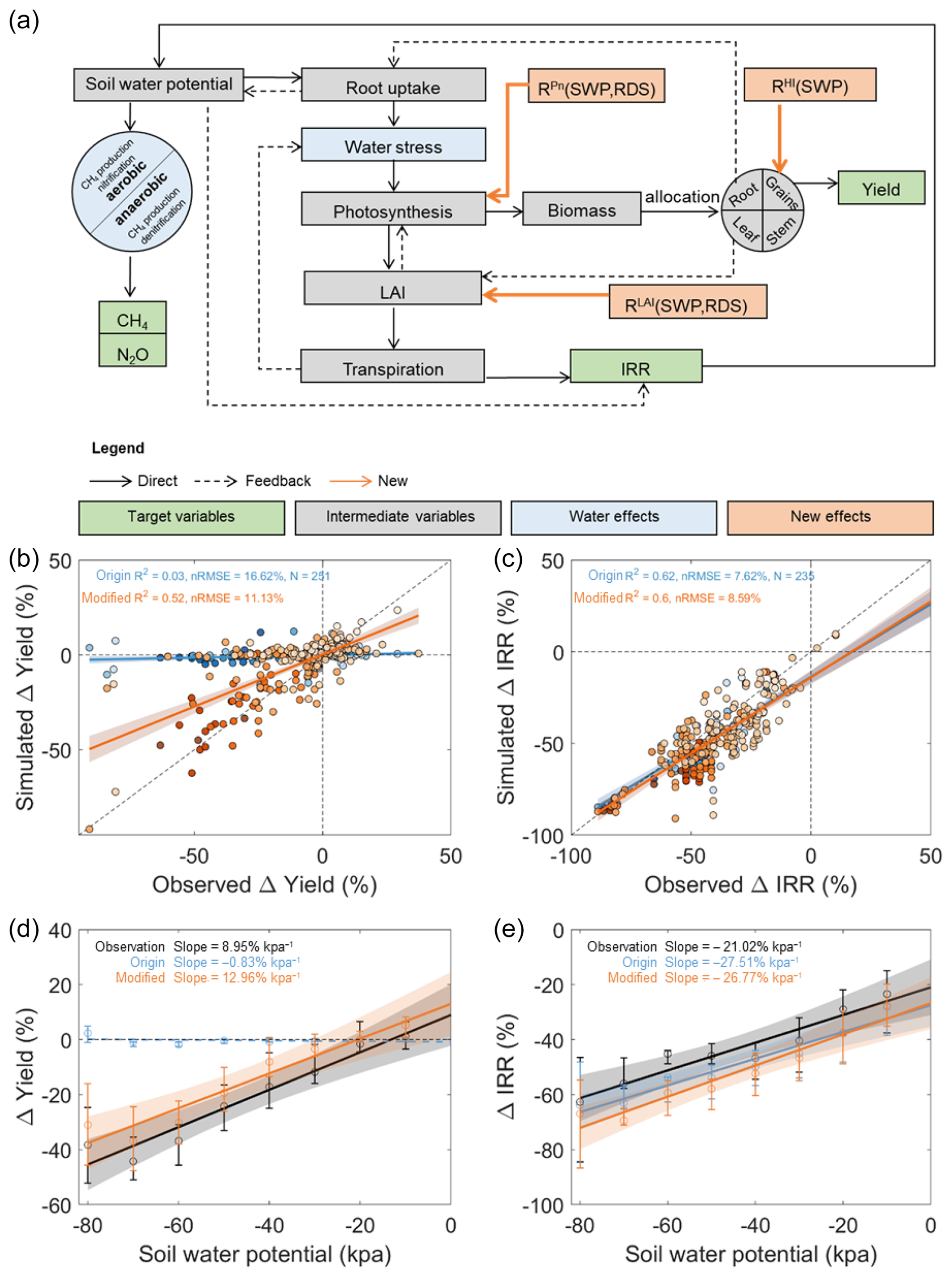
Figure 2 Model improvements by incorporating water effects on physiological processes. (a) Schematic of critical physiological effects in response to different irrigation schemes and their representation in the WHCNS model. (b, c) Model performance for simulating Δyield (b) and ΔIRR (c) based on the origin (blue) and modified (orange) WHCNS model. Darker colored dots indicate lower soil water potential (unit: kPa). (d, e) Sensitivity of Δyield and ΔIRR to lower irrigation threshold of soil water potential. Black, blue, and orange colors show the results of observations and simulations based on the origin and modified WHCNS model, respectively. The circles are mean values; error bars show the 25 %–75 % interquartile range. The lines are the linear regression lines, with dashed lines indicating non-significant relationships based on a two-sided t test (P>0.05). The shaded areas around each line represent the 95 % confidence interval.

2.3.2 Contribution analysis

Scenario simulations were conducted to isolate the contributions of the three physiological effects on yield changes (Δyield) (Table S5). Four scenarios were simulated by considering all the three effects (Table S5) and omitting one of the three effects at a time (Table S5). For each scenario, the model was run under CF and NCF conditions, respectively, to calculate Δyield. The differences in the simulated Δyield between S1 and S2–S4 represent yield changes induced by changes in leaf expansion, photosynthesis rate, and assimilate partition, respectively (i.e., Δyield^LAI, Δyield^Pn, Δyield^HI). The relative contribution of each process was calculated as the ratio of the absolute yield change induced by the process to the sum of the absolute yield changes induced by the three processes (Eq. 13).

$$\begin{array}{}\text{(13)}& {\mathrm{CON}}^p={\displaystyle \frac{\left|\mathrm{\Delta }{\mathrm{yield}}^p\right|}{{\sum }_{p=\mathrm{1}}^{\mathrm{3}}\left|\mathrm{\Delta }{\mathrm{yield}}^p\right|}}\times \mathrm{100},\end{array}$$

where p represents the three new physiological processes (i.e., p= 1, 2, 3), CON^p indicates the relative contribution of the process p to Δyield, and Δyield^p is the yield change induced by the process p.

2.4 Parameters regionalization

Spatially explicit model parameters are critical for reasonably reproducing spatial variability of target variables. In this study, seven key model parameters were selected and mapped at 0.5° spatial resolution due to their high influence on target variables, including accumulated temperature for crop maturity (Cumtemp), minimum assimilation rates (AMIN), the maximum CH₄ production rate per soil weight at 30 °C (MPmax), the maximum portion of denitrification to N₂O production ($f_{{\mathrm{N}}_{\mathrm{2}}\mathrm{O}\mathrm{\_}\mathrm{d}}$), and the three new genetic parameters (P^LAI, P^Pn, P^HI). These parameters were first finely calibrated at site scales (Sect. 2.4.1) and then upscaled to regional scales (Sect. 2.4.2). To capture spatial variability of NCF effects, different parameters were used under CF and NCF conditions, except for the genetic parameters. This was consistent with a previous modeling study, aiming to indicate different potentials of methane production and denitrification under different water management regimes (Song et al., 2023).

2.4.1 Calibration of site-scale parameters

Under CF conditions, the parameter Cumtemp was first determined by cultivar as the minimum cumulative daily temperature higher than 10 °C (base temperature for rice growth) across all experiments using the cultivar. Then AMIN, MPmax, and $f_{{\mathrm{N}}_{\mathrm{2}}\mathrm{O}\mathrm{\_}\mathrm{d}}$ were calibrated to achieve the best fit of predicted target variables with observations under continuous flooding conditions (i.e., experimental control). Under NCF conditions, Cumtemp and AMIN were the same as those calibrated from CF conditions. The other parameters (MPmax, $f_{{\mathrm{N}}_{\mathrm{2}}\mathrm{O}\mathrm{\_}\mathrm{d}},P^{\mathrm{LAI}}$, P^Pn, and P^HI) were then calibrated by minimizing the sum of simulated squared residuals under non-continuous flooding conditions (Table S6). To obtain more accurate parameter estimates, the advanced parameter estimation algorithm (PEST) was used (Doherty, 2010). As a result, 51 groups of genetic parameters (Cumtemp, AMIN, P^LAI, P^Pn, and P^HI), 56 parameter values of MPmax (19 for control and 37 for treatment), and 24 parameter values of $f_{{\mathrm{N}}_{\mathrm{2}}\mathrm{O}\mathrm{\_}\mathrm{d}}$ (10 for control and 14 for treatment) were calibrated.

2.4.2 Parameter upscaling

To upscale genetic parameters (AMIN, Cumtemp, P^LAI, P^Pn, P^HI) calibrated at site scales to regional scales, the rice cultivar for each grid was first determined. Then, the calibrated genetic parameters of the cultivar were used to create the grid. Since the spatial distribution of rice cultivars is unknown, the cultivar of each grid cell was determined as follows. First, cultivars with Cumtemp lower than the effective accumulative temperature requirement of the grid were identified. This ensures that the cultivar could reach maturity under the grid cell's temperature conditions. The grid's temperature requirement was calculated as Cumtemp during rice growing periods specified by the crop calendar data of GGCMI phase 3 (Jägermeyr et al., 2021). Subsequently, cultivars with AMIN that closely match the baseline AMIN of the grid cells were selected. The baseline AMIN was estimated using PEST to achieve the best fit of the yield simulation with the records in the county-scale statistical yearbooks of China (downscaled to 0.5° spatial resolution). These procedures were designed to ensure that yield simulations were aligned with the cultivar's genetic potential and were spatially consistent with observations.

To upscale parameters MPmax and $f_{{\mathrm{N}}_{\mathrm{2}}\mathrm{O}\mathrm{\_}\mathrm{d}}$, two parameter transfer functions (PTFs) were developed. The dependent variables were the ratio of site-calibrated parameters under treatment to those under control (i.e., R^MPmax and $R^{f_{{\mathrm{N}}_{\mathrm{2}}\mathrm{O}\mathrm{\_}\mathrm{d}}}$) (Eqs. 14–15). The independent variables were determined as field water capacity (FWC) for R^MPmax and bulk density (BD) for $R^{f_{{\mathrm{N}}_{\mathrm{2}}\mathrm{O}\mathrm{\_}\mathrm{d}}}$, due to their higher correlations with the dependent variables. The function forms were determined as the form with the highest R². As a result, the relationship between field water capacity and R^MPmax was best fitted by an exponential function (R²= 0.62, p<0.001), and the relationship between bulk density and $R^{f_{{\mathrm{N}}_{\mathrm{2}}\mathrm{O}\mathrm{\_}\mathrm{d}}}$ was best fitted by a quadratic function (R²= 0.91, p<0.001) (Fig. S5). The importance of soil properties in regulating spatial heterogeneity of denitrification potentials aligns with previous studies (Tang et al., 2024). Parameters of the PTFs were calibrated using the least squares method (Eqs. 14–15). With the calibrated PTFs, the ratio of parameters under NCF relative to CF (R^MPmax and $R^{f_{{\mathrm{N}}_{\mathrm{2}}\mathrm{O}\mathrm{\_}\mathrm{d}}}$) for each grid could be predicted by combining a spatial dataset of FWC and BD. Then, gridded MP_max and $f_{{\mathrm{N}}_{\mathrm{2}}\mathrm{O}\mathrm{\_}\mathrm{d}}$ for CF conditions (MP${}_{\max }^{\mathrm{CF}}$ and $f_{{\mathrm{N}}_{\mathrm{2}}\mathrm{O}\mathrm{\_}\mathrm{d}}^{\mathrm{CF}}$) were estimated using PEST, targeting CH₄ from the EDYGA v8.0 dataset (Crippa et al., 2024), and N₂O emissions estimated by Cui et al. (2024) (Fig. S4). These parameters were estimated for 2013 and 2015 and subsequently validated for 2014 and 2016 to assess their ability to reproduce the spatial variability of target variables (Fig. S3). Finally, MP_max and $f_{{\mathrm{N}}_{\mathrm{2}}\mathrm{O}\mathrm{\_}\mathrm{d}}$ for NCF conditions were calculated by multiplying MP${}_{\max }^{\mathrm{CF}}$ and $f_{{\mathrm{N}}_{\mathrm{2}}\mathrm{O}\mathrm{\_}\mathrm{d}}^{\mathrm{CF}}$ with the predicted ratio (R^MPmax and $R^{f_{{\mathrm{N}}_{\mathrm{2}}\mathrm{O}\mathrm{\_}\mathrm{d}}}$).

$$\begin{array}{}\text{(14)}& {\displaystyle }{R}^{{\mathrm{MP}}_{\max }}={\mathrm{MP}}_{\max }^{\mathrm{NCF}}/{\mathrm{MP}}_{\max }^{\mathrm{CF}}=\mathrm{986}\times e^{-\mathrm{26}\times \mathrm{FWC}},\text{(15)}& {\displaystyle }\begin{array}{rl}{R}^{f_{{\mathrm{N}}_{\mathrm{2}}\mathrm{O}\mathrm{\_}\mathrm{d}}}& =f_{{\mathrm{N}}_{\mathrm{2}}\mathrm{O}\mathrm{\_}\mathrm{d}}^{\mathrm{NCF}}/f_{{\mathrm{N}}_{\mathrm{2}}\mathrm{O}\mathrm{\_}\mathrm{d}}^{\mathrm{CF}}=\mathrm{268}\\ & \times {\mathrm{BD}}^{\mathrm{2}}+\mathrm{789}\times \mathrm{BD}+\mathrm{581}\end{array},\end{array}$$

where R^MPmax and $R^{f_{{\mathrm{N}}_{\mathrm{2}}\mathrm{O}\mathrm{\_}\mathrm{d}}}$ represent the ratio of the parameter MPmax and $f_{{\mathrm{N}}_{\mathrm{2}}\mathrm{O}\mathrm{\_}\mathrm{d}}$ calibrated under non-continuous flooding (treatment) to that under continuous flooding (control). FWC and BD represent field water capacity (cm³ cm⁻³) and soil bulk density (g cm⁻³) obtained from SoilGrids (10 km) (Han et al., 2015).

To prove the efficacy of the PTFs, two other parameter upscaling approaches were also used for comparison, including the mean parameters approach and the spatial proximity approach. These approaches were widely used in previous modeling studies to derive regional parameters and conduct regional simulations (Zhang et al., 2024). To adopt the mean parameter approach, the mean value of the site-calibrated MPmax and $f_{{\mathrm{N}}_{\mathrm{2}}\mathrm{O}\mathrm{\_}\mathrm{d}}$ (Sect. 2.4.1) was calculated, respectively, for CF and NCF conditions, and then the two constant mean parameters were used in regional simulations. To adopt the spatial proximity approach, the nearest site of a site was first identified according to geographical coordinates. Then, both MPmax and $f_{{\mathrm{N}}_{\mathrm{2}}\mathrm{O}\mathrm{\_}\mathrm{d}}$ calibrated from the nearest site were used for simulation of this site. The three approaches were compared in their performance to reproduce the observed variations in ΔCH₄ and ΔN₂O (Fig. 3).

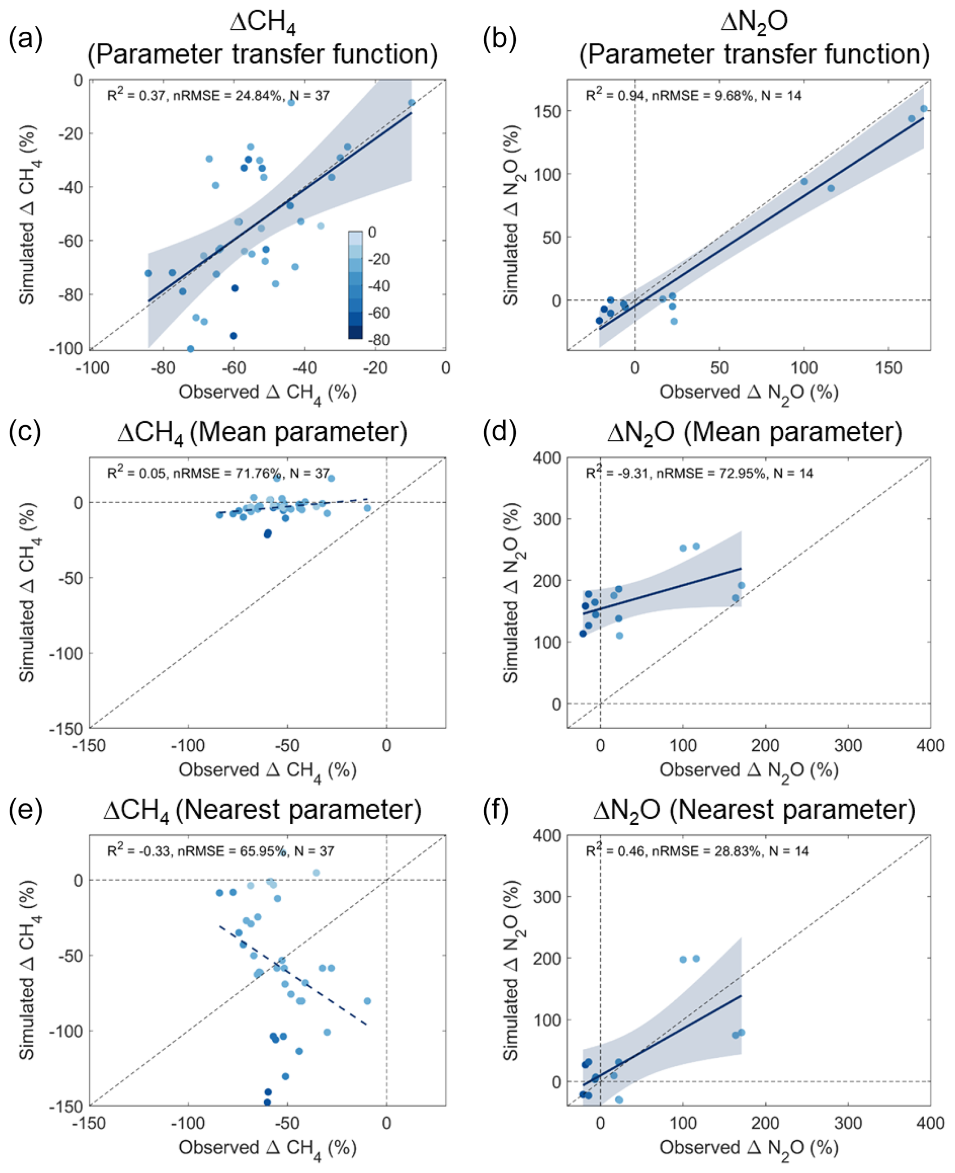
Figure 3 Comparison of model parameter upscaling approaches. Model performance in simulating methane and nitrous oxide emissions changes based on parameters derived from (a, b) parameter transfer functions (PTFs), (c, d) mean site-calibrated parameters, and (e, f) spatially nearest parameters. The color of the dots indicates lower irrigation thresholds of soil water potential under non-continuous flooding irrigation (unit: kPa). The solid lines are regression lines, with dashed lines indicating non-significant relationships (P>0.05). Blue shading around each line represents the 95 % confidence interval.

2.5 Regional scenario simulations and driver identification

Scenario simulations were conducted to test whether the proposed framework could reasonably predict the response sensitivity of target variables and their relations under different irrigation schemes. To do so, the well-calibrated WHCNS model was run under the baseline and a series of non-continuous irrigation scenarios using the parallel computing framework (Liang et al., 2023). For the baseline condition, irrigation thresholds were set according to Chen et al. (2022). For non-continuous flooding irrigation scenarios, a range of the lowest irrigation threshold levels were set based on observations (−5, −10, −15, −20, −30, −40, and −50 kPa). The upper irrigation thresholds were kept the same as the baseline for consistency with experiments. NCF effects were then calculated from model simulations and compared with observed effects. Observed effects were obtained from two datasets. The first is the one compiled for this study (Sect. 2.2) using soil water potential to distinguish irrigation schemes. The second was obtained from Bo et al. (2022), who used the ratio of days with no surface water to total growing days (UFR) to differentiate irrigation schemes. To facilitate comparison, the UFR of each irrigation scenario was also calculated and output by WHCNS (Fig. S9).

To identify the dominant factor driving spatial patterns of NCF effects, correlation analyses between simulated NCF effects and variables were performed following Cui et al. (2021). Climatic, soil, and management-related factors were selected as independent variables, including T, P, ET, Clay, BD, SOC, and fertilizer rate. The analyses were conducted, respectively, for Δyield, ΔIRR, ΔCH₄, and ΔN₂O using 3.5° by 3.5° moving windows. The data resolution was 0.5° by 0.5°, meaning the surrounding 49 pixels were used for each grid. The correlation coefficient and its significance in each grid were first calculated and the dominant driver was then defined as the factor with the largest absolute correlation coefficient. To assess the robustness of the results, similar analyses were done with moving windows at higher spatial resolutions (e.g., 2.5° by 2.5°).

2.6 Single-objective and multi-objective optimizations

Based on scenario simulations, four single-objective and a multiple-objective were designed to identify optimal irrigation schemes. The four single-objective targets are (1) maxYield, which maximizes rice yield; (2) minIRR, which minimizes irrigation water use; (3) minCH₄, which minimizes CH₄ emissions; and (4) minN₂O, which minimizes N₂O emissions. Under all targets, yield reduction compared to CF conditions was avoided. With the optimal solution under the four single-objective scenarios, the largest regulation potentials to increase yield and reduce IRR, CH₄, and N₂O emissions were assessed. For comparison, the scenario simulations and optimization were also conducted using the original WHCNS model (Fig. 5).

The multi-objective optimization was conducted by combining the improved WHCNS model and the NSGA-II (Deb et al., 2002). First, a set of 100 parental populations was initialized with random solutions. Each population includes 1993 individuals, corresponding to 1993 grid cells of irrigated rice areas. Second, the objective functions were computed with each solution by executing the WHCNS model (Eq. 16). Third, the performance of each population was evaluated by ranking the fitness of its objective functions. Fitness is a measure of how well a solution performs and is calculated based on the non-dominated sorting rank. Then, a new generation was generated through selection, crossover, and mutation based on fitness. Finally, Pareto fronts were generated after 100 generations had been evaluated (that is, 10 000 populations).

$$\begin{array}{}\text{(16)}& {\displaystyle }{f}_{\mathrm{objective}}=\left[\begin{array}{l}{f}_{\max }\mathit{\left\{}\sum _{n=\mathrm{1}}^N\mathrm{WHCNS}\right(\mathrm{yield}\left)\mathit{\right\}}\\ f_{min}\mathit{\left\{}\sum _{n=\mathrm{1}}^N\mathrm{WHCNS}\right(\mathrm{IRR}\left)\mathit{\right\}}\\ f_{min}\mathit{\left\{}\sum _{n=\mathrm{1}}^N\mathrm{WHCNS}\right(\mathrm{GWP}\left)\mathit{\right\}}\end{array}\right],\text{(17)}& {\displaystyle }\begin{array}{rl}\mathrm{WHCNS}\left(\mathrm{GWP}\right)& =\mathrm{27.2}\times \mathrm{WHCNS}\left({\mathrm{CH}}_{\mathrm{4}}\right)\\ & +\mathrm{273}\times \mathrm{WHCNS}\left({\mathrm{N}}_{\mathrm{2}}\mathrm{O}\right),\end{array}\end{array}$$

where f_objective (yield, IRR, and GWP) denotes the collection of objective functions, f_max denotes the objective that needs to be maximized (e.g., rice yield), and f_min denotes the objective that needs to be minimized (e.g., IRR and GWP). GWP is the integrated global warming potential of combined emissions of CH₄ and N₂O and is calculated based on WHCNS simulations (Eq. 17) (IPCC, 2021). It should be noted that this study set equal weight for each target variable to evaluate the fitness of each solution. Decision-makers can simply set the weight values of different objectives according to their preferences to adopt advanced multi-objective decision-making methods such as the efficiency coefficient method (Guo et al., 2021). The regulation potentials of multiple-objective optimization were calculated as the averaged NCF effects (Δyield, ΔIRR, ΔCH₄, ΔN₂O, ΔGWP) of all non-dominated solutions. The potentials were further compared with those from single-objective optimizations to investigate tradeoffs between target variables (Fig. 6).

3 Results and discussion

3.1 Performance of model improvement

The origin WHCNS model was first evaluated in reproducing variabilities of rice yield and irrigation water use under various irrigation schemes. For rice yield, model performance is satisfying when mixing observations under continuous flooding (CF, experimental control) and non-continuous flooding (NCF, experimental treatments) irrigation schemes together (R²= 0.41, normalized root mean square error, nRMSE = 11 %) (Fig. S6). In particular, with fine-tuned crop genetic parameters (i.e., Cumtemp and AMIN), the origin model performed well under CF conditions (R²= 0.74, nRMSE = 13 %), while it had worse performance under NCF conditions (R²= 0.22, nRMSE = 13 %) (Fig. S6). As a consequence, the origin model failed to reproduce variations in observed yield changes (Δyield) (R²= 0.03, nRMSE = 17 %) (Fig. 2b). More importantly, the simulations could not reproduce Δyield sensitivities to soil water potentials presented in field experiments (Fig. 2d). In contrast to yield, model performance in simulating irrigation water use responses (ΔIRR) variability and its sensitivities to soil water potentials was acceptable (Fig. 2c and e). These results highlight the primary modeling deficiency in simulating Δyield. Given the satisfying model performance in simulating yield under CF and ΔIRR, the underperformance is likely due to a lack of critical physiological processes responsible for yield responses to NCF rather than uncertainties of crop parameters.

After incorporating the three functions of NCF effects and fine calibration of genetic parameters (Sect. 2.3, Fig. 2a), the model performance was substantially improved. The explained variabilities of Δyield increased from 3 % to 52 % and nRMSE decreased from 17 % to 11 % (Fig. 2b). The observed Δyield sensitivities to soil water potential (9 % kPa⁻¹, P < 0.001) could be reasonably reproduced by the modified model (13 % kPa⁻¹, P < 0.001) rather than the origin model (P > 0.05) (Fig. 2d). The cultivar differences of yield responses could also be simulated (R= 0.67) (Fig. S7). Across the three processes, leaf area growth (Δyield^LAI) was primarily responsible for yield losses, while net photosynthetic rate (Δyield^Pn) and biomass translocation (Δyield^HI) contributed to yield increases (Sect. 2.3.2, Fig. S8). The positive contributions are larger in warmer and more humid areas and in acidic soils with larger field water holding capacity and higher SOC. These findings conform with empirical relationships between Δyield and environmental factors reported by previous meta-analysis (Carrijo et al., 2017). These results prove the efficacy of the modified model to predict and regulate Δyield under diverse irrigation schemes and environmental conditions.

Besides being coupled to WHCNS as an integrated system, the new functions also contribute to advancing related modeling studies by directly involving positive physiological effects and considering stage-dependent response sensitivities (Li et al., 2017). By contrast, most prevailing crop models only account for negative effects of soil drying and reduced transpiration, while they do not incorporate direct compensation effects (such as increased photosynthesis rate upon rewatering). Moreover, constant stress sensitivity parameters were generally used for all growth stages (such as ORYZA and DSSAT) (Bouman et al., 2001; Tsuji et al., 1998). These models could flexibly incorporate the three new functions and recalibrate the genetic parameters (i.e., P^LAI, P^Pn, and P^HI) following the procedures of this study to improve their performance in predicting yield responses.

3.2 Performance of regionalized parameters

To simulate regional NCF effects, the model was first run for CF (baseline) and NCF conditions, respectively, using the parallel computing framework at a spatial resolution of 0.5°. NCF effects were then calculated using model simulations following Eq. (1) (Fig. 1 and Sect. 2.4). Using the PEST-calibrated gridded model parameters for CF (Sect. 2.4.1), the nRMSE between model simulations and their spatial datasets was 20 % to 29 % for yield, ∼ 7 % for IRR, ∼ 4 % for CH₄, and 4 % to 6 % for N₂O during the validation period (year 2014 and 2016) (Fig. S2). It was noted that the nRMSE of rice yield was relatively larger than that of other target variables, despite being within an acceptable range (< 30 % for the validation periods). This could be caused by interannual cultivar changes, which were difficult to consider in large-scale simulations due to the lack of spatial distribution of rice cultivars. Overall, these results reveal a satisfying model calibration to simulate baseline values and spatial variabilities of target variables.

To reproduce observed variabilities of NCF effects on target variables, NCF effects on key model parameters (MPmax and $f_{{\mathrm{N}}_{\mathrm{2}}\mathrm{O}\mathrm{\_}\mathrm{d}}$) were incorporated for constraining model simulations. To do so, NCF effects on model parameters were first quantified from site-scale calibrations and extrapolated to regional scale (Sect. 2.4). Three approaches of parameter extrapolation were tested and compared, including developing parameter transfer functions (PTFs), using mean site-calibrated parameters (mean), and using spatially nearest calibrated parameters (spatial) (Sect. 2.4.3). Results showed that developing PTFs performed the best to reproduce observed variabilities of ΔCH₄ and ΔN₂O (Fig. 3). Model simulations using parameters estimated by PTFs explained 37 % and 94 % of variations in ΔCH₄ and ΔN₂O, with nRMSE being 25 % for ΔCH₄ and 10 % for ΔN₂O (Fig. 3a–b). By contrast, simulations based on the other two approaches could hardly reproduce observed variabilities of ΔCH₄ and ΔN₂O, with nRMSE achieving 66 % to 72 % for ΔCH₄ and 29 % to 73 % for ΔN₂O (Fig. 3c–f). These results prove the efficacy of the developed PTFs and suggest soil variables as good predictors for spatial extrapolation of site-calibrated parameters to simulate CH₄ and N₂O. The PTFs could also be referred by other biogeochemical models for regional simulations of CH₄ and N₂O (such as the Denitrification–Decomposition model and the Dynamic Land Ecosystem Model) (Zhang et al., 2016).

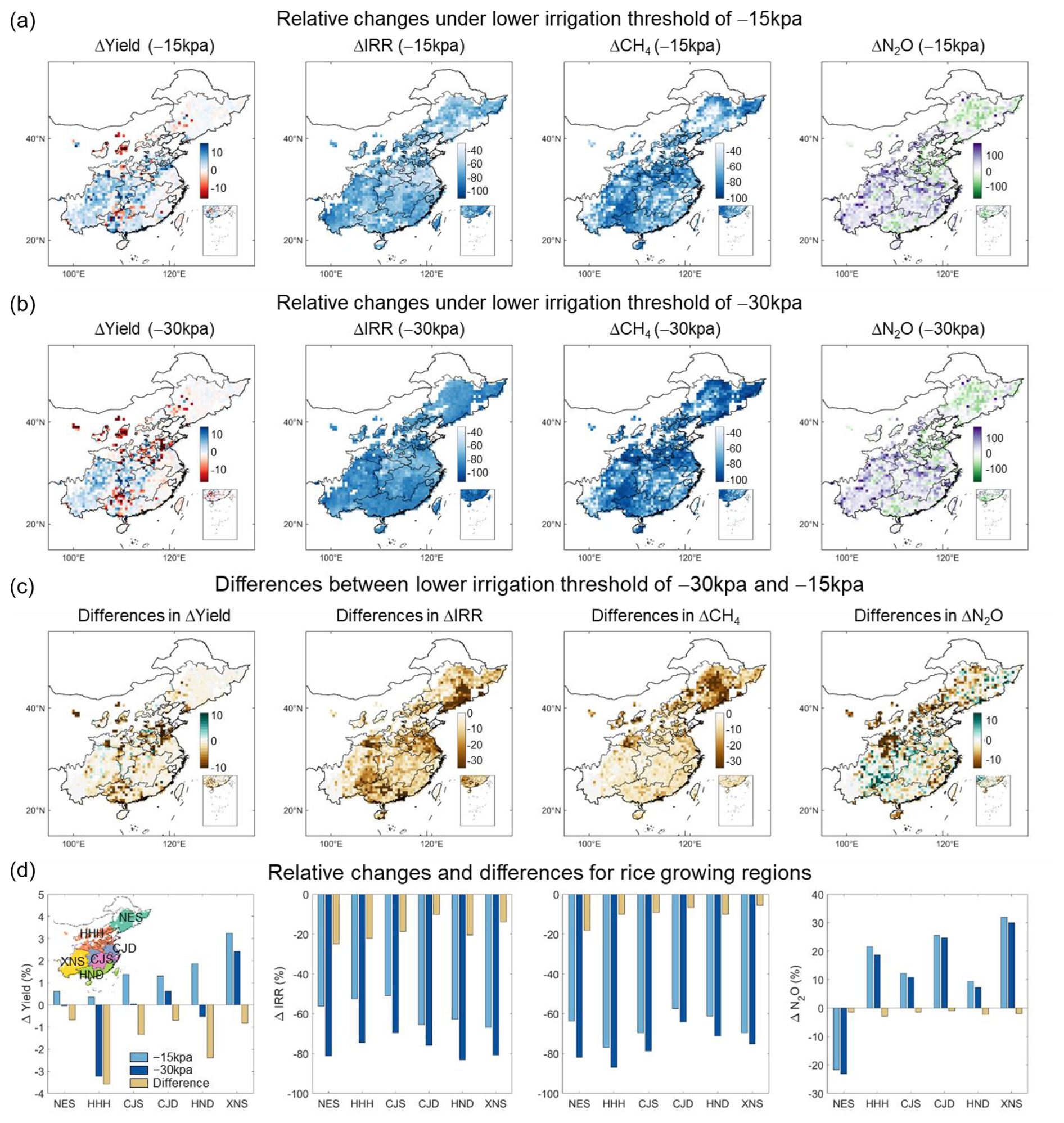
Figure 4 Spatial pattern of relative changes in target variables under different irrigation schemes. The four columns correspond to the four target variables Δyield, ΔIRR, ΔCH₄, and ΔN₂O, respectively. (a) Relative changes in target variables under a lower irrigation potential of −15 kPa, (b) relative changes in target variables under a lower irrigation potential of −30 kPa, (c) differences between (b) and (a), and (d) the results for different rice growing regions. NES (northeast single rice), HHH (HuangHuaiHai single rice), CJS (Yangtze River single rice), CJD (Yangtze River double rice), HND (South China double rice), and XNS (Southwest China single rice) represent six major rice-growing areas in China, respectively. Publisher's remark: please note that the above figure contains disputed territories.

Considering scarce observations of NCF effects across space, it was impractical to directly evaluate the regionalized parameters in reproducing spatial variability of NCF effects. Therefore, the proposed framework was evaluated in terms of the response sensitivity of target variables and their relationships under different irrigation schemes (Sect. 2.5). Scenario simulations broadly conformed with observations regarding the magnitude of NCF effects and response sensitivity across soil water potential gradients (Fig. S9). With decreased soil water potential threshold, Δyield decreased quasi-linearly, ΔCH₄ and ΔIRR decreased at a decelerating rate, while ΔN₂O showed slight variabilities (Fig. S9a). The decelerating decrease in ΔCH₄ was also observed in experiments, suggesting the model's ability to simulate maximum potentials of CH₄ mitigation (Balaine et al., 2019). The response sensitivity was further validated using an alternative observation dataset (Fig. S9b). Besides, the observed synergy or tradeoffs of the yield–IRR–GHGs nexus were broadly covered by scenario simulations using the modified model rather than by using the original model (Fig. S9c). Such bias could further impact assessment of regulation potentials of the food–water–climate nexus.

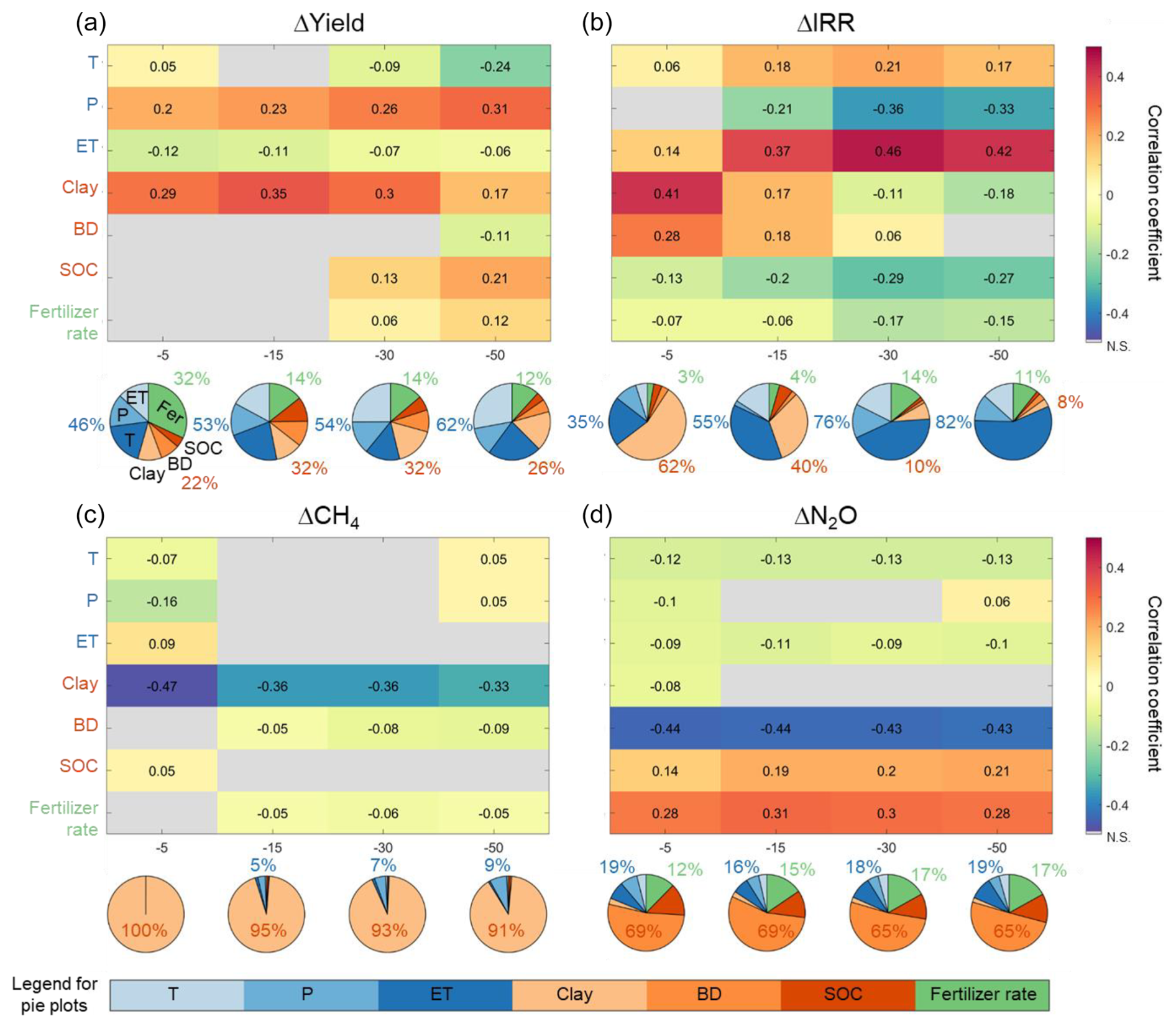
Figure 5 Drivers regulating spatial variations in relative changes in yield (a), IRR (b), CH₄ (c), and N₂O (d). The numbers and colors indicate correlation coefficients, with gray indicating non-significant correlations (N.S., P>0.05). The pie plots represent the proportion of irrigated rice areas (%) for which variation in relative changes is regulated by the dominant drivers. The dominant driver is defined as the factor with the largest absolute correlation coefficient in each grid cell, identified based on 3.5° by 3.5° moving windows. The numbers in blue, orange, and green around the pie plots denote the area proportions dominated by climate (i.e., T+P + ET), soil (i.e., Clay + BD + SOC), and management-related (i.e., fertilizer rate) factors under corresponding lower irrigation threshold. Spatial distributions of dominant drivers are shown in Figs. S10 and S11.

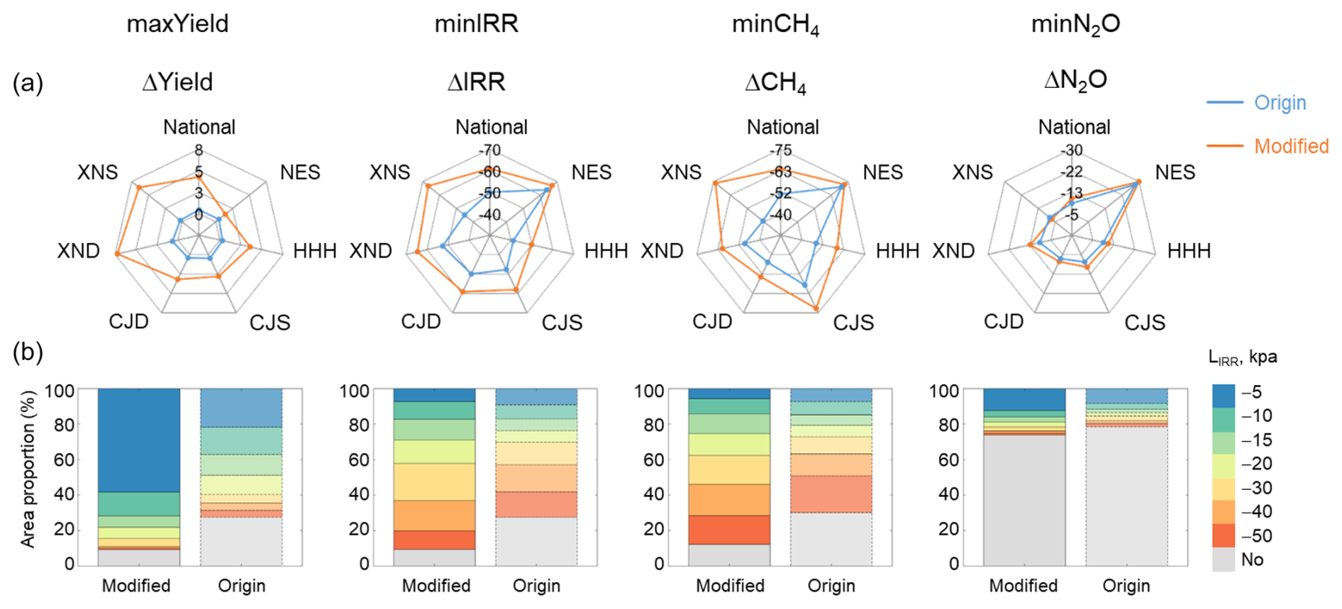
Figure 6 Comparison of the origin and modified model between (a) regulation potentials and (b) optimized irrigation schemes under single-objective targets. The four columns show results under four single-objective targets: maximizing rice yield (maxYield), minimizing irrigation water use (minIRR), minimizing CH₄ emissions (minCH₄), and minimizing N₂O emissions (maxN₂O). (a) Area-weighted Δyield, ΔIRR, ΔCH₄, and ΔN₂O for China and six rice growing regions. Blue and orange indicate results from the origin and modified model, respectively. (b) Proportions of rice areas with corresponding optimized lower irrigation thresholds (L_IRR) to total irrigated rice areas under the four single objective targets. NES, HHH, CJS, CJD, HND, and XNS indicate six rice growing areas of China, namely, northeast single rice, HuangHuaiHai single rice, Yangtze River single rice, Yangtze River double Rice, South China double rice, and Southwest China single rice, respectively.

3.3 Assessment of regional regulation potentials

Scenario simulations revealed large spatial variabilities of NCF effects on all target variables (Fig. 4). Applying the same irrigation scheme (e.g., lower irrigation threshold of −15 or −30 kPa) could induce larger yield increase in the southwestern single-rice region (XNS: 2.4 % to 3.4 %), while larger yield losses in northern regions (HHH: −3.2 %) (Fig. 4a and b). The HHH region also showed larger yield sensitivity with decreased lower irrigation threshold (−0.24 % kPa⁻¹) (Fig. 4c). For IRR, relatively larger water saving benefits occurred in the southern regions, whereas response sensitivity was larger in the northeastern regions (−1.7 % kPa⁻¹). For CH₄, the northern rice growing regions showed relatively higher reductions (NES: 64 % to 82 %, HHH: 77 % to 88 %) and higher response sensitivity to decreased soil water potential threshold. The findings about larger water saving benefits in South China and larger CH₄ mitigation in North China were consistent with previous assessments (Tian et al., 2021). However, N₂O emissions showed widespread increase regardless of lower irrigation threshold, except for northeastern regions, indicating low opportunities to reduce N₂O by only optimizing water management.

To further understand the drivers shaping the spatial variations in NCF effects, correlation analyses were conducted for each target variable across varying lower irrigation thresholds. Overall, climatic and edaphic variables were the most important drivers, while management-related variables were less important (Fig. 5). Exceptions occurred in the southern double rice region (HND) for Δyield and the southwestern single rice region (XNS) for ΔN₂O, where a higher fertilizer application rate was associated with a larger yield increase but decreased N₂O reduction potentials (Figs. S10 and S11). For both Δyield and ΔIRR, clay content was the most important driver at higher irrigation thresholds, while climate factors showed increasing importance with decreased irrigation thresholds (Fig. 5a and b). By contrast, reduction potentials for CH₄ and N₂O emissions were dominated by edaphic factors regardless of irrigation threshold (i.e., clay for CH₄ and bulk density for N₂O) (Fig. 5c and d). These findings highlight the complex interplay of factors influencing regulation potentials of rice production, irrigation water use, and greenhouse gas emissions through NCF adoption.

To identify the largest regulation potentials from NCF adoption, four single objective targets were designed, including maximizing rice yield, minimizing IRR, CH₄ emissions, or N₂O emissions (denoted as maxYield, minIRR, minCH₄, and min N₂O, in Sect. 2.6). Results indicated that the largest regulation potentials of Δyield, ΔIRR, ΔCH₄ and ΔN₂O were 4.6 %, −61.0 %, −64.2 % and −10.9 %, respectively (Fig. 6a). These potentials could be achieved respectively over 91 %, 91 %, 88 % and 26 % of national rice areas (Fig. 6b). Spatially, larger yield increase potential occurred in the south (HND: 7.7 %) and southwestern regions (XNS: 6.8 %) (Fig. S12a). The reduction potential of IRR and CH₄ showed relatively slight spatial variabilities. In contrast, reduction potential of N₂O primarily concentrated in northern regions (NES: −30 %) due to increased N₂O in southern regions (Figs. 5a and S12a). N₂O increase in southern regions is associated with higher nitrogen application rates, providing substrate for nitrification and denitrification processes to facilitate N₂O emissions (Jiang et al., 2019). The results conform to previous studies in that irrigation and nitrogen should be co-regulated for these areas to avoid unintended N₂O emissions from water management (Jiang et al., 2019; Kritee et al., 2018).

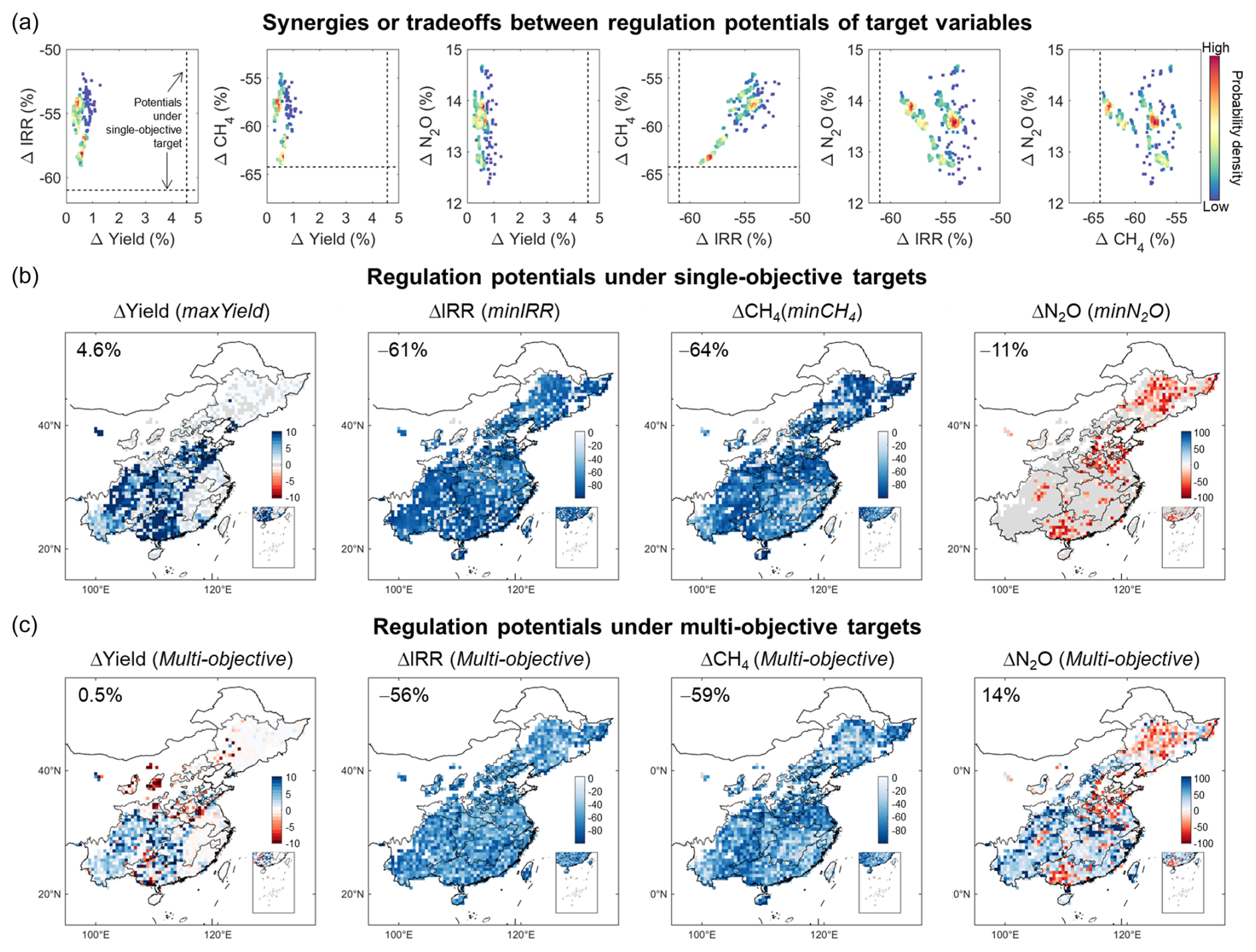
Figure 7 Regulation potentials of Δyield, ΔIRR, ΔCH_4,, and ΔN₂O under single-objective and multi-objective targets. (a) Synergies or tradeoffs between target variables with different solutions of multi-objective optimization. Dot colors indicate probability density distributions of variable changes from all non-dominated solutions (N= 10 000) of the NSGA-II optimization. The vertical and horizontal dashed lines show national regulation potentials of the target variable under single-objective targets, with corresponding spatial distributions presented in panel (b). Note that the results of ΔN₂O potentials (−11 %) were not shown in the third, fifth, and sixth subplots for a clearer view. (b) Δyield, ΔIRR, ΔCH₄, and ΔN₂O under single-objective targets of maximizing rice yield (maxYield), minimizing irrigation water use (minIRR), minimizing CH₄ emissions (minCH₄), and minimizing N₂O emissions (maxN₂O). These results indicate the maximum benefits of each target variable from adopting non-continuous irrigation, which could not necessarily be realized simultaneously. (c) Δyield, ΔIRR, ΔCH₄, and ΔN₂O under multi-objective optimization. These figures show mean benefits from all non-dominated solutions of the NSGA-II optimization (N= 10 000). Publisher's remark: please note that the above figure contains disputed territories.

The largest regulation potentials of Δyield, ΔIRR, ΔCH_4, and ΔN₂O are not likely to be achieved at the same time, as evidenced by different optimized irrigation strategies between single-objective targets (Figs. 6 and S13). For example, the lower irrigation threshold should be higher than −20 kPa for most areas (84 %) under maxYield, while lower than −20 kPa over half areas under minIRR and minCH₄. This suggests tradeoffs between yield increase and IRR/CH₄ mitigation (Bo et al., 2022). To compare, using the origin model could overlook nearly 20 % feasible areas for applying optimized irrigation schemes (Fig. 6). As a consequence, regulation potentials of Δyield, ΔIRR, ΔCH₄, and ΔN₂O could be underestimated by 4 %, 11 %, 14 %, and 2 %, especially for the southwestern regions (XNS) (Fig. 6a). Moreover, optimal NCF strategies also differed from those identified by the improved model, particularly under maxYield targets (Fig. 6b). These results showed important implications of the improved framework for prompting sustainable water management.

3.4 Tradeoffs between food, water, and greenhouse gas emissions

The NSGA-II was conducted to investigate synergies or tradeoffs of the food–water–climate nexus (Fig. 7 and Sect. 2.6). There were evident tradeoffs between reducing CH₄ (or IRR) and N₂O (Fig. 7a). In contrast, synergies were noted between reducing IRR and CH₄, and between inhibiting N₂O emissions and increasing rice yield. The relationships between yield increase and CH₄ (or IRR) reductions were more complicated due to the impacts of varying irrigation timing and no-flooded days (Yan et al., 2024). Adopting non-dominated solutions from multi-objective optimization could realize over 90 % of the largest reduction potentials of IRR and CH₄, while at the cost of 4 % less yield increase (4.6 % versus 0.5 %) and 25 % higher nitrous dioxide emissions (−11 % versus 14 %). The N₂O increase is because this study used integrated warming potentials of CH₄ and N₂O emissions (GWP) to indicate greenhouse gas emissions so that CH₄ outweighed N₂O due to large emission quantities (Sect. 2.6).

Spatially, over 90 % of the reduction potentials for IRR and CH₄ could be achieved across 53 % and 60 % of the national rice areas, primarily in southern regions (Figs. 7 and S14). In these areas, N₂O increase was inevitable, but yield increase could be expected. By contrast, stronger tradeoffs occurred in the northern regions, where the reduction potentials of IRR and CH₄ were limited even with decreased yield and increased N₂O emissions. Therefore, NCF adoption should be prioritized in southern regions (e.g, XND, CJD, and CJS) to achieve a national optimum balance among rice production, water use, and greenhouse gas emissions mitigation. Note that other objective functions could also be designed for multi-objective optimization, such as applying other indicators (e.g., water productivity and yield-scaled GWP), setting distinguished weights for each indicator or grid cell.

3.5 Uncertainties and future direction

This framework is subject to several uncertainties, mainly sourced from observational gaps and management-related input data. First, the absence of field observations for baseline CH₄ and N₂O emissions across regional scales forced us to use estimates from inventory or data-driven approaches as a proxy for deriving gridded model parameters in this study (Cui et al., 2021; Crippa et al., 2024). Despite uncertainties in predicting absolute values, these parameters could reasonably reproduce the spatial patterns and could be further refined given increased field observations. Second, the limited experimental observations of CH₄ (n = 37) and N₂O (n= 14) under various irrigation schemes have contributed to uncertainties in developing and applying parameter transfer functions (PTFs). The values of PTF predictors (bulk density and field water capacity) in the observation dataset (1.34–1.48 g cm⁻³ and 0.25–0.30 cm³ cm⁻³) did not encompass the full range across national rice areas (1.24–1.48 g cm⁻³ and 0.22–0.32 cm³ cm⁻³), indicating potential extrapolation in parameters regionalization (Fig. S1). Despite these uncertainties, the PTFs significantly improved over previous approaches (constant parameters or spatial proximity approach). Lastly, current irrigation practices across large scales remain largely unknown, so that irrigation thresholds were set following previous recommendations. However, actual farmer practices are influenced by various factors and may not align with these recommendations. This discrepancy could lead to an overestimation or underestimation of target variables and further introduce uncertainties to the assessment of regulation potentials.

These uncertainties provide insights to enlighten future research efforts, including conducting extensive observations and experiments and developing high-resolution input data. On the one hand, intensive GHG monitoring networks are essential to reduce uncertainties associated with parameterization (Arenas-Calle et al., 2024). To better constrain the PTFs and reduce extrapolation uncertainty, field experiments combined with incubation experiments across a broader range of climate conditions (e.g., colder and more humid areas) and soil properties (e.g., areas with higher SOC or lower bulk density) should be conducted (Fig. S1). In addition, extensive field experiments with simultaneous measurements of yield, IRR, CH_4, and N₂O emissions across diverse environments are required to validate the framework further. On the other hand, developing a high-resolution dataset of current irrigation schemes is crucial for more accurate model parameter calibration and realistic assessment of regulation potentials. This could be achieved by integrating remote sensing technologies with extensive field investigations (Novick et al., 2022).

4 Conclusion

This study introduced an advancing framework for process-based modeling of the complex food–water–climate nexus in rice fields under various water management schemes. By integrating the Soil Water Heat Carbon Nitrogen Simulator (WHCNS) with key physiological effects, a novel model upscaling method, and the NSGA-II multi-objective optimization algorithm at a parallel computing platform, the framework provides a comprehensive approach to optimize irrigation strategies. Applying this framework to China's rice cropping system, we assessed the largest regulation potentials of Δyield, ΔIRR, ΔCH_4,, and ΔN₂O as 4.6 %, −61.0 %, −64.2 %, and −10.9 % from 91 %, 91 %, 88 %, and 26 % of national rice areas. However, these regulation potentials could not be simultaneously realized due to complicated tradeoffs among food–water–GHGs. Based on NSGA-II multi-objective optimization targeting food–water–GHG co-benefits, over 90 % of the reduction potentials in water use and methane emissions could be realized, while at the cost of 4 % less yield increase and 25 % higher nitrous dioxide emissions. The proposed framework is a valuable tool for irrigation optimization in rice cultivation and also offers a transferable paradigm for incorporating other management effects into process-based models, thus supporting comprehensive assessments of sustainable management measures.

Appendix A

Table A1 Abbreviation table of parameters and variables.