An updated non-intrusive, multi-scale, and flexible coupling interface in WRF 4.6.0

The Weather Research and Forecasting (WRF) model has been widely used for various applications, especially for solving mesoscale atmospheric dynamics. Its high-order numerical schemes and nesting capability enable high spatial resolution. However, a growing number of applications are demanding more realistic simulations through the incorporation of coupling with new model compartments and an increase in the complexity of the processes considered in the model (e.g., ocean, surface gravity wave, land surface, and chemistry). The present paper details the development and the functionalities of the coupling interface we implemented in WRF. It uses the Ocean–Atmosphere–Sea–Ice–Soil Model Coupling Toolkit (OASIS3-MCT) coupler, which has the advantage of being non-intrusive, efficient, and very flexible to use. OASIS3-MCT has already been implemented in many climate and regional models. This coupling interface is designed with the following baselines: (1) it is structured with a two-level design through two modules: a general coupling module and a coupler-specific module, allowing for easy additions of other couplers if required; (2) variable exchange, coupling frequency, and any potential time and grid transformations are controlled through an external text file, offering great flexibility; and (3) the concepts of external domains and a coupling mask are introduced to facilitate the exchange of fields to/from multiple sources (different models, fields from different models/grids/zooms, etc.). Finally, two examples of applications of ocean–atmosphere coupling are proposed. The first is related to the impact of ocean surface current feedback to the atmospheric boundary layer, and the second concerns the coupling of surface gravity waves with the atmospheric surface layer.

1 Introduction

The Weather Research and Forecasting (WRF, Skamarock, 2004) model is probably among the most popular atmospheric regional model with more than 50 000 users in 160 countries. This state-of-the-art non-hydrostatic atmospheric model is used in a wide range of atmospheric research and operational forecasting applications at scales ranging from thousands of kilometers to tens of meters. WRF's success can be explained in many ways (easy configuration setup, a large and active community, etc.), but the key feature of this model is definitely the quality of its results thanks to the extended choice of available physical parameterizations and to its dynamic solver (ARW, Skamarock and Klemp, 2008) that was especially designed with high-order numerical schemes to enhance the model's effective resolution of mesoscale dynamics. Another popular feature of WRF is its capability to nest, which allows for running a part of the model domain at higher spatial resolution. These nests can be defined either at the same level (sibling nests) or nested within each other to a certain depth (parent–children nests). The position of the nest within the parent grid can be fixed in time or can move, either along a specified trajectory or following a predefined criterion (e.g., low in the 500 mb height).

The WRF community continually proposes new contributions to improve and/or add features to the model. One way of improving the quality and realism of numerical simulations is to refine the representation of physical processes in the model. This can be achieved by increasing the level of detail and complexity of modeled processes or incorporating new processes or even new model compartments into the system. Following the example of the climate modeling community, which started to use coupled models more than 50 years ago (Manabe and Bryan, 1969), there is a growing number of applications using regional atmospheric models such as WRF coupled with another model such as ocean, surface gravity wave, land surface, or chemistry. WRF has been coupled to numerous ocean models, notably the Coastal and Regional Ocean Community Model (CROCO, Renault et al., 2019a), the MIT General Circulation Model (MITgcm, Sun et al., 2019), the Nucleus for European Modelling of the Ocean (NEMO, Samson et al., 2014), the Princeton Ocean Model (POM, Liu and al 2011), the Hybrid Coordinate Ocean Model (HYCOM, Chen et al., 2013), the Parallel Ocean Program (POP, Cassano et al., 2017), or the Regional Ocean Modeling System (ROMS, Warner et al., 2010).

Coupling WRF with another model can simply be achieved by exchanging data through files (e.g., Jullien et al., 2014); however, most coupled models nowadays use a coupler, which allows for direct data exchange, offering better performances and more flexibility, particularly with regards to grid interpolation. Today, WRF is therefore coupled using the most common couplers, such as, for example, the Earth System Modeling Framework (ESMF, Hill et al., 2004); the Community Coupler (C-Coupler, Liu et al., 2014); the Model Coupling Toolkit (MCT, Larson et al., 2005), either directly or through CPL7 (Craig et al., 2012) or through the Ocean–Atmosphere–Sea–Ice–Soil Model Coupling Toolkit v5 (OASIS3-MCT version 5, Craig et al., 2017), as detailed in the present paper. Each coupler has its own benefits and drawbacks, with none being universally suitable for all constraints, requirements, and practices of the various groups that employ them. Valcke (2022) classifies them into two main categories: the external coupler or coupling library (typically C-Coupler and OASIS3-MCT) and the integrated coupling framework (typically ESMF and CPL7). WRF incorporates a coupling interface with one representative from each of these two categories: ESMF (already in WRF version 3) and OASIS3-MCT (since version 3.6 in 2014). The main objective of this publication is to provide an extensive description and user guide of this OASIS-MCT coupling interface. The update of this interface, phased with WRF 4.6.0, has motivated the writing of this paper, which fills the gap in the documentation of this work we initiated a decade ago. Note that all changes made to the code are available on GitHub at the following address: https://github.com/massonseb/WRF/commits/GMD_wrf_coupling/?author=massonseb (last access: 8 November 2024). They are limited to a few routines, so porting them to older versions of WRF will be fairly straightforward.

The OASIS3-MCT coupler was designed to easily couple various models with minimal changes required to the models being coupled. Often described as the “Swiss army knife” coupler, OASIS3-MCT is a set of libraries, which allows for variable exchange between different models and performs grid interpolations and time transformations if requested by the user (see the OASIS3-MCT user guide for all details; Valcke et al., 2021). OASIS3-MCT is fully parallelized (thanks to the MCT engine), ensuring good computational performance. It has the advantage of being non-intrusive (only a few calls in the model time stepping, and a few additional calls for communicators, grids and subdomains' definition) and very flexible to use. Once the coupling interface has been implemented into the code, the users can define their coupling strategy (which variables are exchanged with what spatial and temporal treatment) directly through an external text input file, allowing for flexibility without requiring any additional adjustments to the source code. The qualities of OASIS3-MCT explain its high popularity and its use in seven of CMIP6 global climate models as well as in various components of regional models (see examples at https://oasis.cerfacs.fr/en/results-of-the-survey-2019-on-oasis3-mct-coupled-models/, last access: 21 June 2021). WRF has thus been coupled through this interface with various models, including the chemistry-transport model CHIMERE (Briant et al., 2017), the land surface model ORCHIDEE (Guion et al., 2022), the surface gravity wave model WAVEWATCH III (Tolman, 2009), the coastal ocean model FVCOM (Kayastha et al., 2023), or the previously mentioned ocean models CROCO and NEMO.

The ocean–atmosphere coupling is by far the most popular application of this work, which has already been used in numerous studies. Many of them showed the importance of the air–sea coupling at oceanic (sub)mesoscale in various regions: the Agulhas Current (Renault et al., 2017), the Bay of Bengal (Krishnamohan et al., 2019), the California Current (Renault et al., 2016a, 2018), the English Channel (Renault and Marchesiello, 2022), the Gulf of Mexico (Larrañaga et al., 2022), the Gulf Stream (Renault et al., 2016a, 2019c), the Mediterranean Sea (Renault et al., 2021), the south-eastern Pacific (Oerder et al., 2016, 2018), the tropical Atlantic (Gévaudan et al., 2021) or even the entire tropical channel (Jullien et al., 2020; Renault et al., 2019c, 2020, 2023). Other studies used this coupling interface to focus on tropical cyclones (e.g., Samson et al., 2014; Lengaigne et al., 2019; Neetu et al., 2019) or the Indian monsoon (Samson et al., 2017; Terray et al., 2018). The Model of the Regional Coupled Earth System (MORCE, Drobinski et al., 2012) platform is also benefiting from this coupling interface. MORCE was used in diverse projects such as Med-CORDEX (Ruti et al., 2016) with application in the local atmospheric dynamic (Drobinski et al., 2018) or extreme meteorological events (Lebeaupin Brossier et al., 2015; Berthou et al., 2016; Panthou et al., 2018).

The present paper describes in detail the implementation and the usage of the OASIS3-MCT coupling interface in WRF. In Sect. 2, the general philosophy of the non-intrusive and flexible interface is given. Its detailed implementation in the code, the changes to the original code to add the coupling interface and the few modifications needed to activate the coupling interface at the compilation stage are detailed. In Sect. 3, different applications of the interface are illustrated, along with the few additional changes to the WRF original code. Finally, in Sect. 4, the ability of this tool to go towards multi-scale applications is exposed, with the implemented concept of a coupling mask allowing for the coupling of various domains, including embedded zooms or not.

2 A non-intrusive and flexible coupling interface

The design of this coupling interface was motivated by the idea of limiting modifications to the original WRF code as much as possible in order to facilitate its maintainability. To do so we used the OASIS3-MCT coupler (Craig et al., 2017), which requires very few intrusions into the code, and we adopted a few coding rules:

• Isolate the interface itself in dedicated new modules, module_cpl.F and module_cpl_oasis3.F (which are detailed in Sect. 2.1).

• Limit the modifications to the original code by only adding calls to coupling subroutines.

• Distinguish these coupling subroutines with a name starting with cpl_.

• Mark off and control the calls to these subroutines with a test on a logical, named coupler_on.

The implementation is fully detailed in Sect. 2.4, but let's first introduce the overall philosophy of our coupling strategy.

2.1 A two-level coupling interface

The coupling interface was written to be used with OASIS3-MCT. However, one could argue that the main steps of the coupling are quite generic and applicable to most couplers. We therefore structured our coupling interface with a two-level design through two modules: a generic coupling module, frame/module_cpl.F, and a dependency module for the chosen coupler, frame/module_cpl_oasis3.F.

The first module, frame/module_cpl.F, gathers all the subroutines called in the other parts of the code. This module is thus the only coupling module “used” in the other original WRF routines (i.e., with the Fortran instruction USE module_cpl). Its public subroutines constitute the set of generic actions that should be required by the coupler. This module is always compiled, even if the user is not doing any coupling, along with other WRF modules. We tried to limit the use of C preprocessor keys, which tend to create “dead code” over time. This also makes the code easier to read by limiting the preprocessing command lines and ensures that the coupling interface is compiled when new modifications are made to the code (and therefore checked obvious bugs).

In this module, we define the logical coupler_on and the string of characters coupler_name which defines the coupler we are using, as shown in Fig. 1.

Figure 1 Declaration of coupler_on and coupler_name in frame/module_cpl.F.

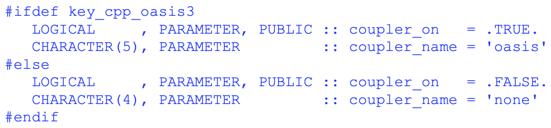
As of today, the only implemented coupler using this interface is OASIS3-MCT. The choice of the definition of coupler_name is thus limited to two cases: 'none' or 'oasis', but the structure of frame/module_cpl.F is designed to add more choices.

The OASIS3-MCT-specific interface is isolated and defined in a separate new module: frame/module_cpl_oasis3.F. This second module is the only location where we use OASIS3-MCT routines. It is thus the only file containing the following call to OASIS module:

USE mod_oasis ! OASIS3-MCT module

The public routines of frame/module_cpl_oasis3.F are only used in frame/module_cpl.F, which minimizes the intrusion of OASIS3-MCT into WRF code. The use of the C preprocessor key key_cpp_oasis3 ensures that this routine can be compiled without key_cpp_oasis3 and generates, in this case, dummy routines allowing for the compilation of frame/module_cpl.F.

2.2 The coupling sequence

The coupling sequence (Fig. 2) is structured into three steps with functionalities corresponding to specific Fortran subroutines provided in the coupling interface that are callable from the original code:

• Initialization and definition phase. Take care of message passing interface (MPI) communicators and MPI subdomains definition.

• Temporal loop and exchange phase. Potentially receive/send data from/to the coupler at the beginning/end of each time step.

• End of simulation. Finalize or abort coupling.

The initialization, definition and finalization steps are done once in each model outside of the temporal loop, while the send/receive interfaces are called at every time step (Fig. 2). Nevertheless, the effective exchanges of data between two models are done at the coupling time step that is usually larger than the model time step (e.g., 1 h). This coupling time step, which must be a common multiple of each model time step, is defined by the user in an external text file read by the coupler (see next sub-section). An example of a coupling sequence is illustrated in Fig. 3, featuring two models with distinct time steps, dt₁ and dt₂. In this example, the coupling time step is 2 times dt₁ and 4 times dt₂.

In forced mode, WRF reads the surface boundary conditions at the beginning of the time step. In coupled mode, these quantities are provided by the coupler. In the real world, the air–sea exchanges are continuous, but it is not easy to achieve such synchronicity in coupled models. The cleanest way would be to iterate the coupling procedure several times at each coupling time window until flux computation converges (Lemarié et al., 2015). The computational cost of this methodology is, however, prohibitive. A compromise could be to have a coupling time step small enough to represent the continuous air–sea exchanges. This solution is often not compatible with the relatively large time step of ocean models and the uncertain validity over small time windows (< 10 min) of bulk formulations that have been calibrated using average hourly measurements (Large, 2006). The usual solution is to exchange averaged fields over a coupling time window that is considered small enough to represent a kind of synchronicity while being compatible with the ocean model time step and the bulk formulations. To obtain the best compromise between numerical performance and the coherence of the coupling fields, the ocean and atmospheric models run in parallel rather than sequentially (see Fig. 4 of Valcke, 2013) using dedicated MPI resources (see details on MPI communication in Sect. 2.4 and MPI resource allocation in Sect. 2.6). The atmosphere modifies the ocean state which will not provide feedback to the atmosphere immediately but with a delay of the coupling time window. In OASIS3-MCT, a functionality called lag is used to synchronize the send and receive functions and avoid deadlock between models (detailed in Sect. 2.5.3 of the OASIS3-MCT user guide; Valcke et al., 2021). In our implementation, the sending function is called at the end of the time step, and the receiving function is called at the beginning. Synchronous exchanges therefore require sending to take place during the time step preceding reception, which is ensured by defining the lag as one time step of the sending model. Note that at the beginning of the simulation, the variables to be received are read in NetCDF restart files written by the sending models at the end of the previous simulation.

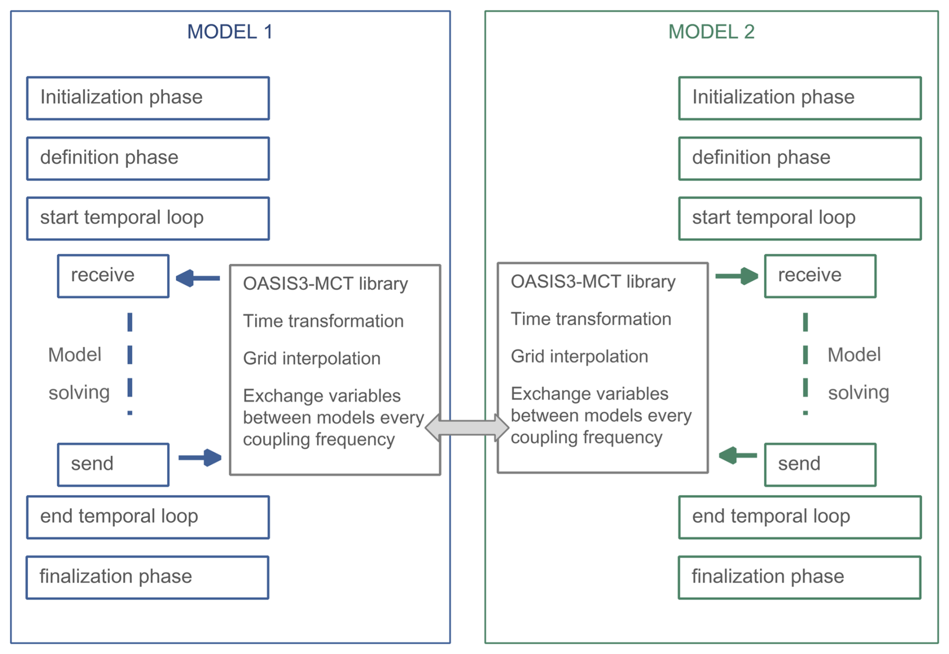
Figure 2 Schematic view of the coupling steps implemented in the WRF coupling interface: initialization, definition, exchanges and finalization. Here, an example of two models coupled through OASIS3-MCT is illustrated.

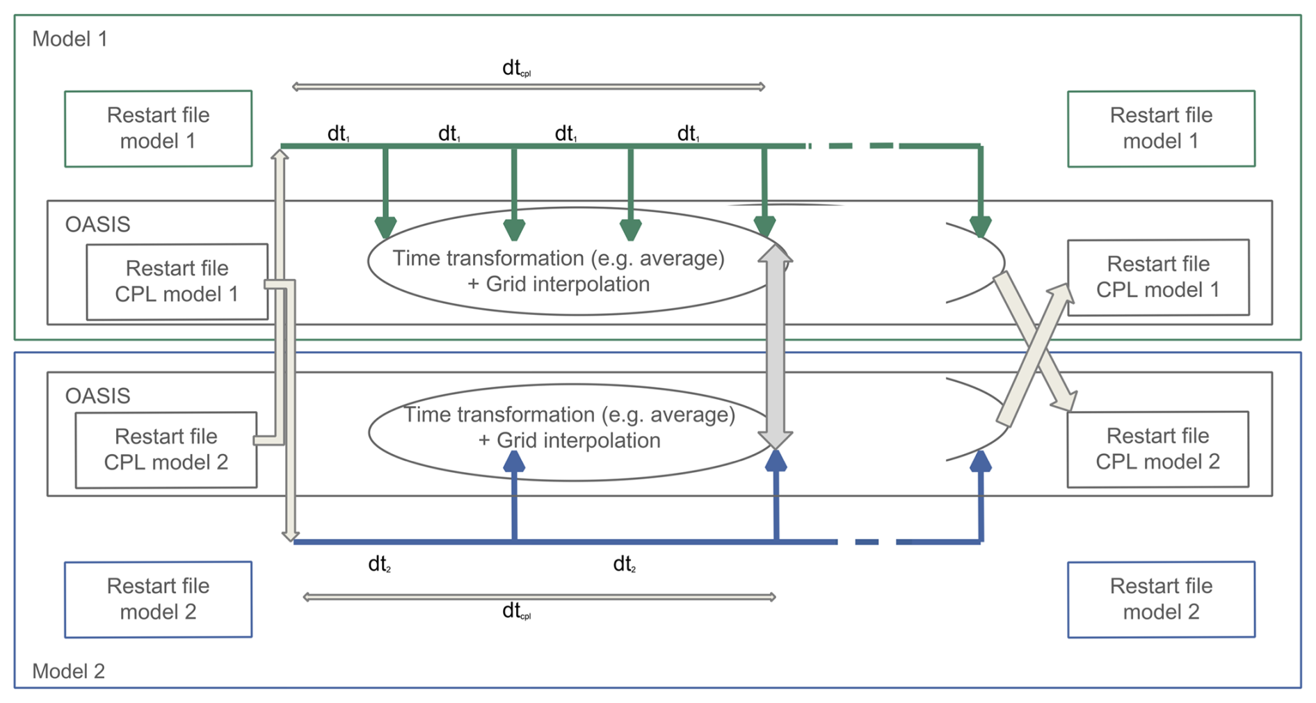
Figure 3 Schematic view of the coupling sequence used in a coupled simulation between two models interfaced using the OASIS3-MCT library.

2.3 A coupling strategy controlled by an external file

Following OASIS3-MCT approach, the coupling interface is further configured through a simple external text file which allows for the setup of the coupled simulation without modifying or recompiling the code. In the OASIS3-MCT coupler, this file is called the namcouple. It allows for a complete configuration of the coupled simulation by specifying

• which variable will be exchanged,

• to/from which domain,

• at which frequency,

• with which temporal treatment and spatial interpolation.

The list of variables potentially sent or received by WRF is hard-coded in the subroutine cpl_init of frame/module_cpl.F. However, this does not necessarily mean that they will be used or coupled. The variables to be coupled are selected in the namcouple file and, in WRF, for each potential coupling variable, we check whether it is actually required in the user-defined namcouple. Each coupling variable is identified through a name, which is hard-coded and stored in a character array, named either rcvname (received) or sndname (sent) and defined as private variables of the module frame/module_cpl.F. The maximum length of rcvname or sndname names is arbitrarily defined to 64 characters. The current list of these potentially exchanged variables is detailed in Sect. 3.3.

The coupling subroutines designed for the exchanges (cpl_tosend and cpl_toreceive in frame/module_cpl.F) are called at every time step which is, for example, needed to compute the time average or check if it is time to receive some data. Note that, when sending data, all time transformations are performed locally by the model sending data without requiring any MPI communication. The effective exchange of data between models, involving MPI communications, is performed only when the domain integration reaches a coupling time step defined independently for each exchanged variable in the namcouple (Fig. 3).

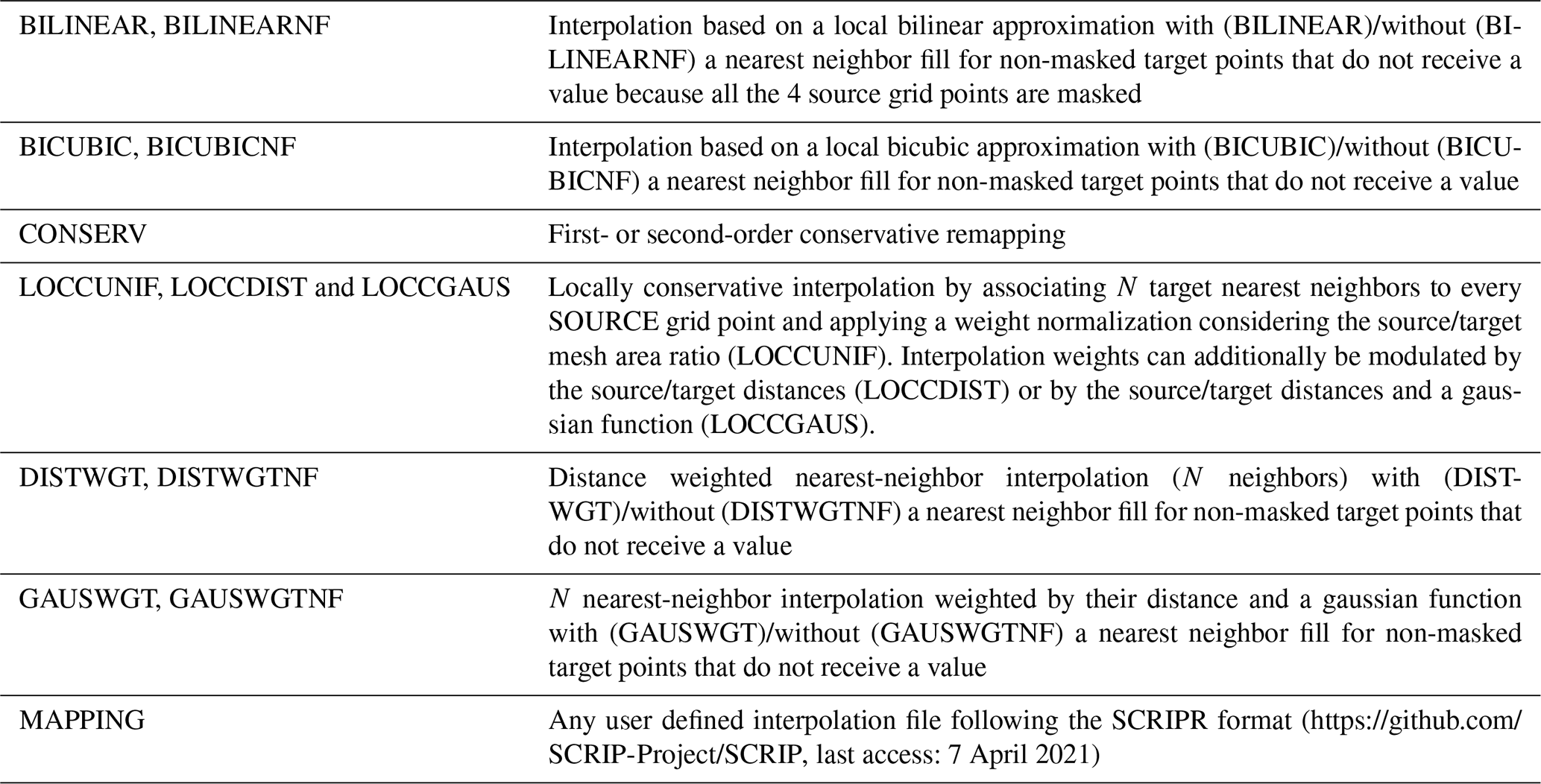
The time transformations and grid interpolation methods available in OASIS3-MCT are summarized in Tables 1 and 2 (see also the OASIS3-MCT user guide for further details; Valcke et al., 2021). All intermediate arrays needed for some of the time transformations (e.g., average) are managed internally and automatically by OASIS3-MCT without any additional code lines in WRF. In the OASIS3-MCT namcouple, users have the option to determine whether spatial interpolations should be applied to time-transformed data by the sending or the receiving model. This strategy provides greater flexibility in optimizing the load balance of the models. OASIS3-MCT can automatically compute interpolation weights for certain spatial interpolations based on input files specifying the grid characteristics (see Valcke et al., 2021, for all details). These input files, called grids.nc, masks.nc and areas.nc, can be automatically built from the WRF geogrid files (i.e., geo_em.dxx.nc, where xx is WRF domain number) using the shell script in Appendix A. Finally, OASIS3-MCT uses a dedicated restart file for each model. Since our model uses quantities accumulated during the previous coupling step, the OASIS restart file contains the initial or restart fields that will be used to initiate or restart a simulation. At the end of the run, OASIS3-MCT automatically writes the new restart files to be used at the start of the next chunk of the simulation.

Table 1 Time transformations available in OASIS3-MCT using the LOCTRANS keyword in the namcouple. See the OASIS3-MCT user guide for more detailed information (Valcke et al., 2021).

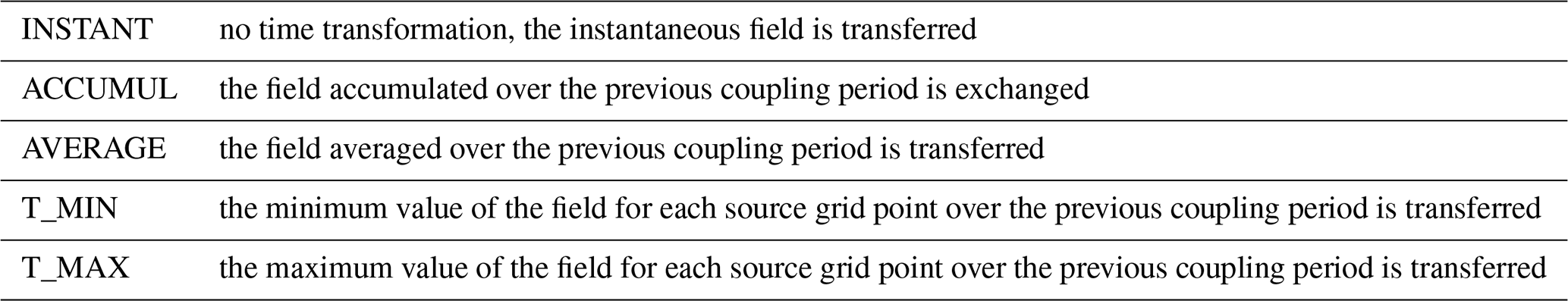
Table 2 Spatial interpolation available in OASIS3-MCT. See the OASIS3-MCT user guide for more detailed information (Valcke et al., 2021).

2.4 Detailed implementation in WRF

In the following, we detail the implementation of the coupling interface in WRF. A schematic representation is also depicted in Fig. 4.

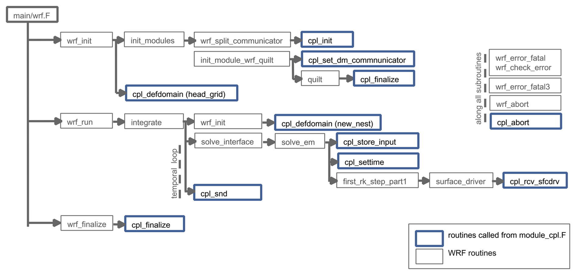
Figure 4 Schematic view of the coupling interface implementation in WRF. WRF original routines are in grey. All new routines (in blue) are gathered in frame/module_cpl.F.

2.4.1 Initialization phase

Defining the MPI communicator

The first task of the coupler is to handle the MPI communicator. This is done in the WRF split_communicator subroutine of external/RSL_LITE/module_dm.F. WRF uses the variable mpi_comm_here as a global communicator, which is defined as MPI_COMM_WORLD by default. When coupling, this MPI communicator is defined by calling the cpl_init subroutine, as shown in Fig. 5.

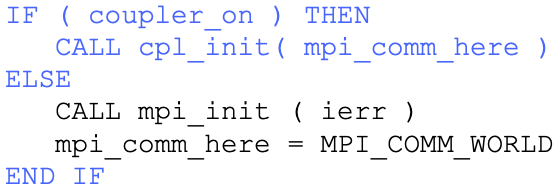
Figure 5 Modification of external/RSL_LITE/module_dm.F to add the call to cpl_init. Lines added for the coupling interface are in blue. Original code lines are in black.

When using OASIS3-MCT as the coupling library, mpi_comm_here is given by OASIS3-MCT, which defines a local communicator for each model, including all the model processes involved in the coupling. The MPI_COMM_WORLD communicator is reserved by OASIS to properly close the simulation. It is also possible to couple through OASIS3-MCT with all components gathered in a single executable. In this case, OASIS3-MCT split the single executable communicator into several communicators, each of them addressing one component. The current implementation of the coupling interface follows the first strategy, which corresponds to the usual usage of OASIS3-MCT that is less intrusive.

An additional step is required when WRF uses its input/output (I/O) quilting. We must indeed specify to the coupler which MPI tasks are dedicated to the model integration (the “computing nodes”) and which are dedicated to the I/O quilting (the “server nodes”). This code modification is done in WRF init_module_wrf_quilt subroutine of frame/module_io_quilt_old.F or frame/module_io_quilt_new.F. Computing nodes send to the coupler their local communicator, mpi_comm_local (defined by wrf_set_dm_communicator) by calling the cpl_set_dm_communicator subroutine, whereas server nodes send the MPI_COMM_NULL communicator to specify to the coupler that they are not included in the coupling, as shown in Fig. 6.

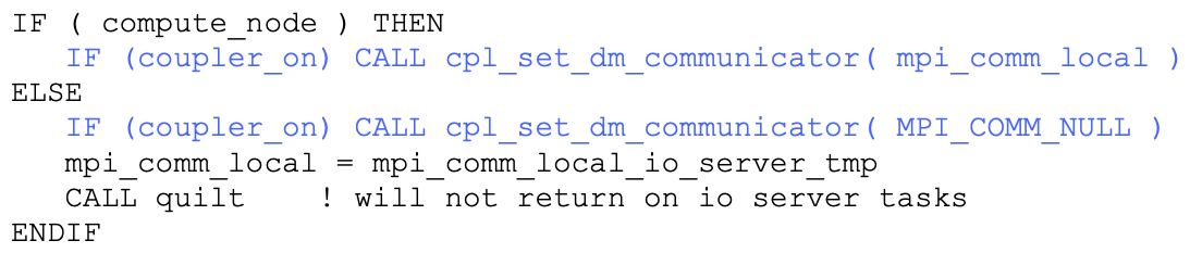
Figure 6 Modification of frame/module_io_quilt_old.F to add the call to cpl_set_dm_communicator. Lines added for the coupling interface are in blue. Original code lines are in black.

Mapping the MPI subdomains

Once the proper MPI communicators are defined, the next step is to provide to the coupler the mapping of the MPI subdomains that identifies which computing node is dedicated to which part of the model grid integration. In WRF, the domain decomposition is defined in alloc_and_configure_domain, which is called at two different places in the code: wrf_init subroutine in main/module_wrf_top.F for the head grid and integrate subroutine in frame/module_integrate.F for the nested child grids. In both cases, the cpl_defdomain subroutine is used to provide the grid definition to the coupler.

For the parent grid, the call to cpl_defdomain is done at the end of the wrf_init subroutine, as shown in Fig. 7.

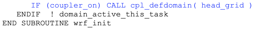
Figure 7 Modification of main/module_wrf_top.F to add the call to cpl_defdomain. Lines added for the coupling interface are in blue. Original code lines are in black.

For the child grids, the call to cpl_defdomain is done at the end of the while loop on the number of children at the beginning of integrate, as shown in Fig. 8.

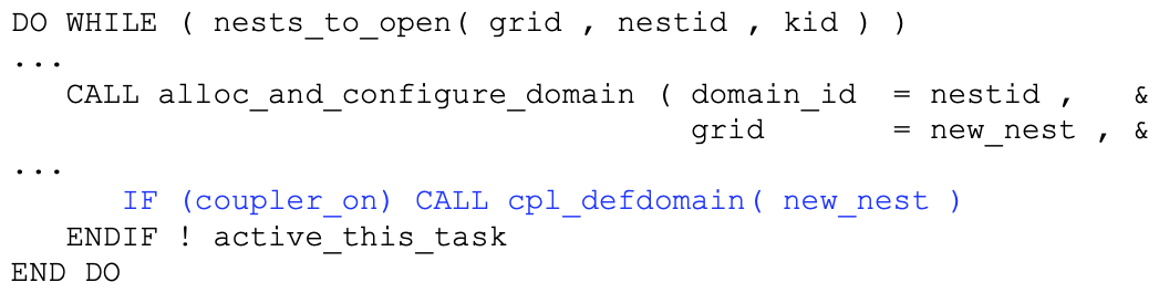
Figure 8 Modification of frame/module_integrate.F to add the call to cpl_defdomain. Lines added for the coupling interface are in blue. Original code lines are in black.

In addition to the grid partitioning, the cpl_defdomain subroutine determines the variable exchange between parent or child domains. This selection of the coupled variables is further detailed in Sect. 3.3.

Note that OASIS3-MCT imposes that all grid and MPI partitioning definitions are done before starting exchanges from/to a given model. This constrain has three consequences regarding the use of nested grids in coupled mode:

1. First, in coupled mode with OASIS3-MCT, all the nested grids must be initiated and ceased at the same time of the parent grid. This is not required in WRF stand-alone mode.

2. Second, as the grid definition must be done only once and before any variable exchange, moving nests can be used but cannot be directly coupled. As detailed in the “Conclusion and discussion” section, they can however be coupled indirectly by coupling only the static parent domain on which the moving nests provide feedback.

3. Third, as presently implemented in WRF, the coupling interface works with a maximum of one level of nested grids. Indeed, in WRF, the definition of the child domains is done at the beginning of the first time step of the parent grid (notably to allow different start/stop dates for nested grid, as mentioned in the first point). Thus, the first level of child grid (whose parent is head_grid) is defined before any exchange, which is ok for OASIS3-MCT. However, as the integrate subroutine is recursive, the second level of the child grid is defined after the first step of the grandparent grid, which is not allowed by OASIS3-MCT. A solution to this limitation is proposed in the discussion.

2.4.2 Temporal loop

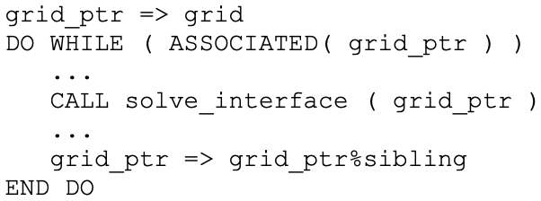
The temporal loop is performed within the recursive integrate subroutine in frame/module_integrate.F with a while loop. The time integration of a single time step is ensured by a call to the solver (dyn_em/solve_em.F in our case), which is applied in a do loop on each sibling domain (i.e., domains at the same level in the zooms hierarchy), as shown in Fig. 9.

Figure 9 Recursive integration of the different nest in frame/module_integrate.F.

Initialization part of the solver

Two calls to the coupling routines are performed in the initialization part of the solver before the call to the first part of the Runge–Kutta scheme. We first call the cpl_store_input subroutine, which eventually copies data that have been read in the AUXINPUT4 input file (wrflowinp_dxx file, with xx representing the domain number) in order to keep a copy of the wrflowinp values before the reception of the corresponding data from the coupler (see Sect. 3.1.2 for additional information):

IF (coupler_on) CALL cpl_store_input
( grid, config_flags )

The cpl_store_input subroutine requires an update of the variable just_read_auxinput4 at the end of the solve_em subroutine to specify if new data have just been read in the AUXINPUT4 input file.

IF (coupler_on) grid%just_read_auxinput4
= Is_ alarm_tstep(grid%domain_clock,
grid%alarms(AUXINPUT4_ALARM))

The second call to coupling routines before the actual integration is the call to cpl_settime, which provides to the coupler the time (in seconds) since the beginning of the simulation (from the cold or hot restart):

IF (coupler_on) CALL cpl_settime(
curr_secs2 )

Exchanging variables

Up to now, all coupling fields defined in the coupling interface are “surface” data (2D arrays) sent by an external domain (i.e., another domain grid than WRF d01, d02, etc.) belonging for example to an ocean, a wave or a land model. These surface data must be received before the calls to the surface parameterizations. The reception of the data sent by the coupler must thus be done at the beginning of the surface_driver subroutine of phys/module_surface_driver.F. This is done by a simple call to the coupling subroutine named cpl_rcv_sfcdrv (for the surface driver), as shown in Fig. 10.

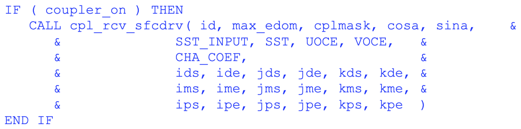
Figure 10 Call to cpl_rcv_sfcdrv that was added in phys/module_surface_driver.F. Lines added for the coupling interface are in blue.

The surface data SST, UOCE, VOCE and CHA_COEF are the output parameters (see Sect. 3.3 for details) of the cpl_rcv_sfcdrv subroutine, whereas all other parameters are intent(in). For each sibling, a recursive call to the integrate subroutine is ensuring that all children are also proceeding their temporal integration by calling solve_em.

Coupling fields are then sent to the coupler at the end of the integrate subroutine once the parent grid time step and the child grid sub-time-step integrations have been performed and once all child domains have given feedback to their parent. The cpl_snd subroutine is called to achieve this task, as shown in Fig. 11.

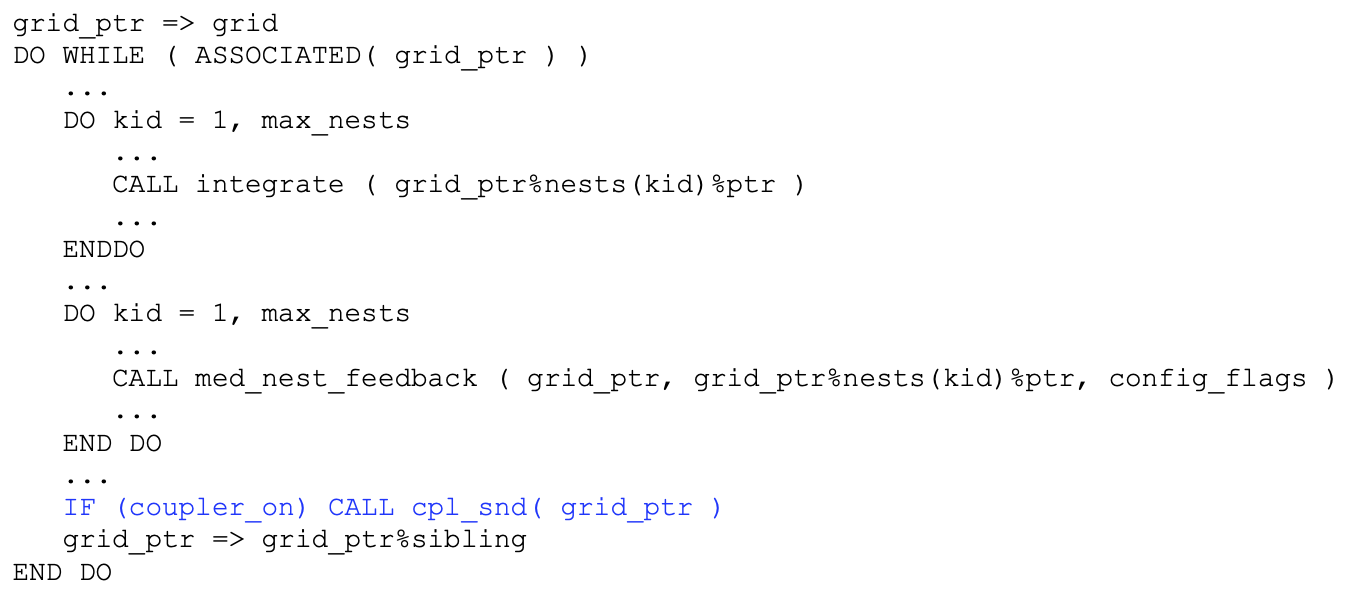
Figure 11 Schematic representation of the while loop on the different nests in frame/module_integrate.F with the added call to cpl_snd. Lines added for the coupling interface are in blue. Original code lines are in black.

2.4.3 End of the simulation

In coupled mode, at the end of the simulation, when reaching the last lines of the wrf_finalize subroutine in main/module_wrf_top.F, the cpl_finalize subroutine is called instead of WRFU_Finalize and wrf_shutdown in stand-alone mode, as shown in Fig. 12.

Figure 12 Added call to cpl_finalize in main/module_wrf_top.F. Lines added for the coupling interface are in blue. Original code lines are in black.

The wrf_abort subroutine in external/RSL_LITE/module_dm.F has also been modified to allow for, in the case of an error, a clean abort of WRF in the coupling interface and a clear associated error message. This prevents for any deadlock in the coupling interface. The dedicated cpl_abort subroutine is thus called in coupled mode instead of the usual mpi_abort (see Fig. 13).

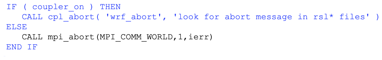
Figure 13 Added call to cpl_abort in external/RSL_LITE/module_dm.F. Lines added for the coupling interface are in blue. Original code lines are in black.

2.5 Compilation

As detailed previously, our coupling interface is structured as a two-level design separating generic coupling routines and coupler-specific routines. This allows for coupling WRF with different couplers. At the current stage, we have only interfaced the OASIS3-MCT coupler, but the procedure should be similar with couplers which require the same kind of input as OASIS, such as YAC (Hanke et al., 2016) or C-Coupler (Liu et al., 2014).

OASIS3-MCT is a set of libraries that has to be downloaded and compiled before compiling WRF (with the same compiler and preferably with the same compiler version; see https://oasis.cerfacs.fr/en/home/, last access: 3 April 2023, for details) and then linked at the end of WRF compilation. Activating the OASIS3-MCT coupling interface in WRF thus requires a dedicated WRF compilation with a few changes in the configure.wrf file:

First, the additional C preprocessor key named key_cpp_oasis3 must be added to the list of keys already defined in the ARCH_LOCAL variable:

ARCH_LOCAL = -Dkey_cpp_oasis3 -D...

Second, the paths to OASIS3-MCT directories containing the library (lib) and the included files (include) must be added so that the compiler knows where to find them. The simplest way to proceed is to follow what is done, for example, for the treatment of NetCDF include and library paths in configure.wrf. First, we define an additional variable OA3MCT_ROOT_DIR, which defines the root directory for OASIS3-MCT:

OA3MCT_ROOT_DIR = /.../oasis3-mct/BLD

Then, we add OASIS3-MCT paths to the list of include modules, as shown in Fig. 14.

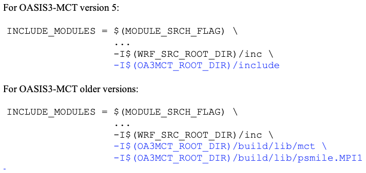
Figure 14 Added path to OASIS3-MCT includes in configure.wrf. Added lines are in blue. Original lines are in black.

Finally, we complete the list of library paths, keeping in mind that it is safer to respect the following rule in the order of the libraries: “if library A depends on library B, library A must be listed before library B”. As OASIS3-MCT depends on NetCDF, the OASIS3-MCT libraries must be listed before NetCDF libraries, as shown in Fig. 15.

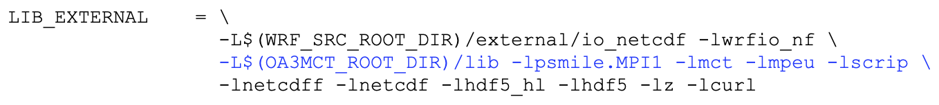
Figure 15 Added path to OASIS3-MCT libraries in configure.wrf. Added lines are in blue. Original lines are in black.

Once these modifications of configure.wrf have been done, WRF can be compiled as usual.

2.6 Running the coupled model

To achieve higher parallelism and keep the different models as independent as possible, each model has its own executable with its dedicated MPI resources. All the executables run in parallel and share the same MPI world using the multiple programs, multiple data (MPMD) launch mode. WRF can be coupled to one or several external models. WRF and the external models can include one or several domains (e.g., embedded zooms, see Sect. 4). For example: if X is the number MPI tasks allocated to WRF and Y the number of MPI tasks allocated to the external model to which WRF is coupled (e.g., an ocean model), the number of MPI tasks that must be allocated to run the simulation is X+Y. Then, if using WRF IO quilting, the X WRF MPI tasks will be split among X1 computing nodes and X2 server nodes, with X= X1 + X2. If WRF is configured with one nested zoom, the parent and the child domains, d01 and d02, will run sequentially on X1 MPI tasks. The same applies to the external model, which could include its own zoom domains running on Y MPI tasks. Note that the external models do not use/see WRF I/O quilting. OASIS3-MCT can couple models sharing the same executable, so we could imagine further integrating WRF I/O quilting in the coupling interface, but this would require specific modifications of the external models and greater entanglement between the different codes, which is not our objective.

3 Ocean–wave–atmosphere coupling and exchanged variables

This section details some of the coupling applications that could be done with the current coupling interface.

3.1 Ocean–atmosphere coupling and, in particular, ocean current coupling with modifications to the PBL schemes

Since a decade ago or so, ocean–atmosphere interactions have been shown to have a large influence not only on the climate but also at smaller scales, such as oceanic mesoscale and submesoscale, with a rectifying effect at a larger scale (Seo et al., 2023). These interactions are mainly driven by two feedback mechanisms from the ocean to the atmosphere: the thermal feedback (TFB), which is the influence of sea surface temperature (SST) gradients and anomalies on the atmosphere, and the current feedback (CFB), which is the influence of sea surface currents on the atmosphere. Coupling the atmosphere with the ocean therefore involves the exchange of several fields. From the atmosphere to the ocean model, the surface heat, water and momentum fluxes are sent. These only require some fields' transformation in the cpl_snd subroutine of module_cpl.F (e.g., computing wind stress components and net heat fluxes) and does not imply any modifications to the original WRF routines. From the ocean to the atmosphere model, the SST and the ocean current components (UOCE, VOCE) are sent to the atmosphere. The SST coupling does not imply any changes to the WRF original routines, while the current feedback to the atmosphere requires a few modifications to both the surface driver and the planetary boundary layer (PBL) parameterization routines (Renault et al., 2019b). Indeed, because of the implicit treatment of the bottom boundary condition, accounting for the relative motion of the atmosphere and the ocean involves a modification of both the surface layer parameterization and the tridiagonal matrix for vertical turbulent diffusion (Lemarié, 2015). In WRF, as the building of the tridiagonal system is done locally in each PBL parameterization, accounting for current feedback thus has to be done for each PBL parameterization. The implementation of the requested modifications has, for now, been done in two popular PBL schemes: the Yonsei University (YSU, Hong et al., 2006) and the Mellor–Yamada–Nakanishi–Niino (MYNN, Nakanishi and Niino, 2009) schemes. The required modifications are summarized in Fig. 16. Samelson et al. (2024) explored the impact of the relative wind in other PBL schemes and proposed the corresponding WRF modifications in the GitHub repository associated with the publication. These modifications have no implications in the case of a WRF stand-alone run as the ocean current velocities (i.e., UOCE and VOCE variables) are set to 0 by default.

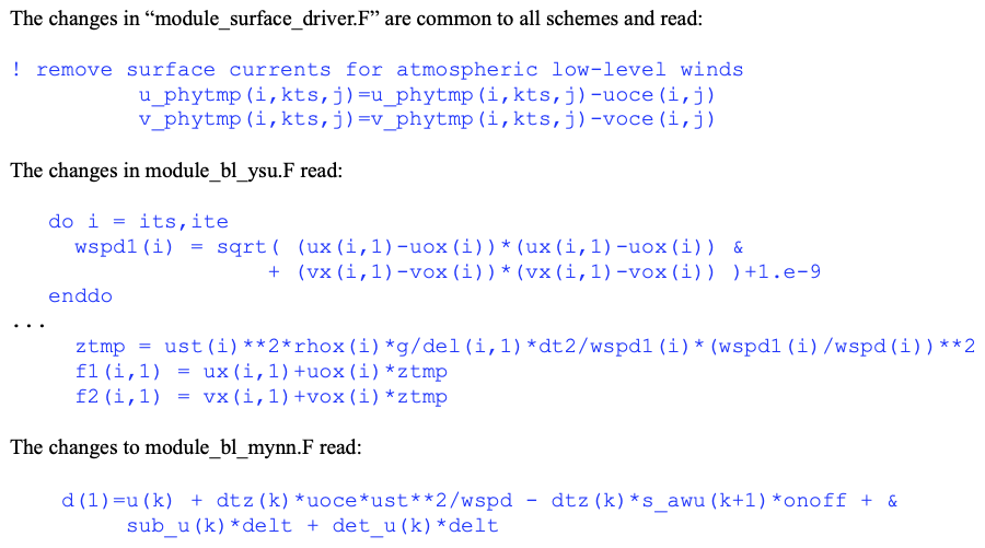
Figure 16 Modifications of phys/module_surface_driver.F, phys/module_bl_ysu.F and phys/module_bl_mynn.F to include ocean currents coupling.

3.2 Atmosphere–wave coupling and modifications to the surface schemes

Atmosphere and surface gravity wave coupling may appear obvious while observing the ocean surface under various wind conditions. In atmospheric models, the wave interface and energy transfers at the air–sea interface are parameterized through a bulk formulation of air–sea fluxes (e.g., Charnock, 1955). However, the underlying mechanisms responsible for atmosphere–wave coupling continue to be a topic of ongoing discussion (e.g., Soloviev and Kudryavtsev, 2010; Hristov, 2018; Ayet et al., 2020). The effect of waves in bulk formulations is also considered an average effect varying only with wind speed, while observations show that the sea state depends on numerous other factors (e.g., wave age, crossed seas and wave–current interactions). One way to account for the variability related to sea state is to incorporate a Charnock coefficient that is dependent on the sea state in the bulk formulation. This can be achieved by either calculating it from a modeled wave spectrum (Janssen et al., 2001) or using it as a function of key wave parameters, such as the wave age or steepness (e.g., Moon et al., 2004; Drennan et al., 2005) or wave height and mean wavelength (e.g., Warner et al., 2010).

Following this approach, we use the Charnock coefficient (CHA_COEF) computed in the wave model to compute roughness length in the WRF surface layer schemes. Like the current feedback, wave feedback to the roughness length requires change in each surface scheme as each scheme computes roughness length locally. Here, the implementation has been performed in the two schemes that use the isftcflx namelist parameter defining alternative drag coefficient Cd formulations: the revised MM5 Monin–Obukhov scheme (Jiménez et al., 2012, sf_sfclay_physics = 1 or 91 in namelist.input) and the MYMM scheme (Olson et al., 2021, sf_sfclay_physics = 5 in namelist.input). Coupling through the exchange of the Charnock coefficient is activated by isftcflx = 5. The changes made in module_sf_mynn.F, module_sf_sfclay.F and module_sf_sfclayrev.F are shown in Fig. 17.

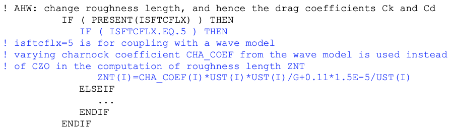
Figure 17 Modifications of module_sf_mynn.F, module_sf_sfclay.F and module_sf_sfclayrev.F to include roughness length coupling. Lines added for the coupling interface are in blue. Original code lines are in black.

Implementation of atmosphere–wave coupling in other surface schemes is not done yet, but as shown here, it only requires a few modifications of the WRF original routines.

Implementing other ways to account for wave feedback, such as using bulk formulations based on wave parameters as the significant wave height, wavelength, wave age or others (e.g., Taylor and Yelland, 2001; Oost et al., 2002; Warner et al., 2010; Sauvage et al., 2023), only requires a few modifications of WRF original routines, similarly to what is performed here, and the addition of new coupled fields in module_cpl.F, similarly to what is performed for CHA_COEF. Note that the MYNN surface scheme (module_sf_mynn.F) already includes options to use parameterizations like those in Taylor and Yelland (2001), which estimate wave parameters from 10 m wind speed and do not incorporate actual wave parameters. Implementing the use of mean wave parameters provided by an actual coupled wave model would therefore be straightforward in this scheme. It would only require receiving the necessary coupled fields in the coupling interface module_cpl.F, similarly to what is performed for CHA_COEF.

3.3 Exchanged variables

The complete list of variables that can be exchanged between WRF and an external model is shown in Tables 3 (received variables) and 4 (sent variables). Extending the list of coupling variables if the proposed set does not meet the user's needs is easy. The maximum number of coupling variables to be potentially sent or received is defined by the parameter max_cplfld in frame/module_driver_constants.F. Its default value (20) can be increased to any size if needed.

Each coupling variable is identified through a name which is hard-coded and stored in a character array: either rcvname or sndname that are private variables of the module frame/module_cpl.F. The maximum length of rcvname or sndname names is arbitrarily defined to 64 characters. For code readability and easy identification of the exchanged variables and of the external domain (i.e., a grid domain other than WRF d01, d02, etc.) from which/to which they are exchanged, we decided that names used to identify coupling variables must be composed of three parts following this convention:

1. Start with WRF_dxx, with xx being a two-digit integer specifying WRF domain number (parent or child) which sends or receives the data.

2. Continue with _EXT_dyy, where yy is a two-digit integer specifying the number of the external domain with which the exchange must be done (see Sect. 4.1 for further details on external domain usage).

3. End with the suffix _XXX, where XXX is a made of any character used to designate the field to be exchanged.

For example, if we want to exchange the sea surface temperature (identified as SST) between the second domain of WRF and the third external domain, we use the following name: WRF_d02_EXT_d03_SST.

Table 3 List of the variables potentially received, in the current version of the coupling interface.

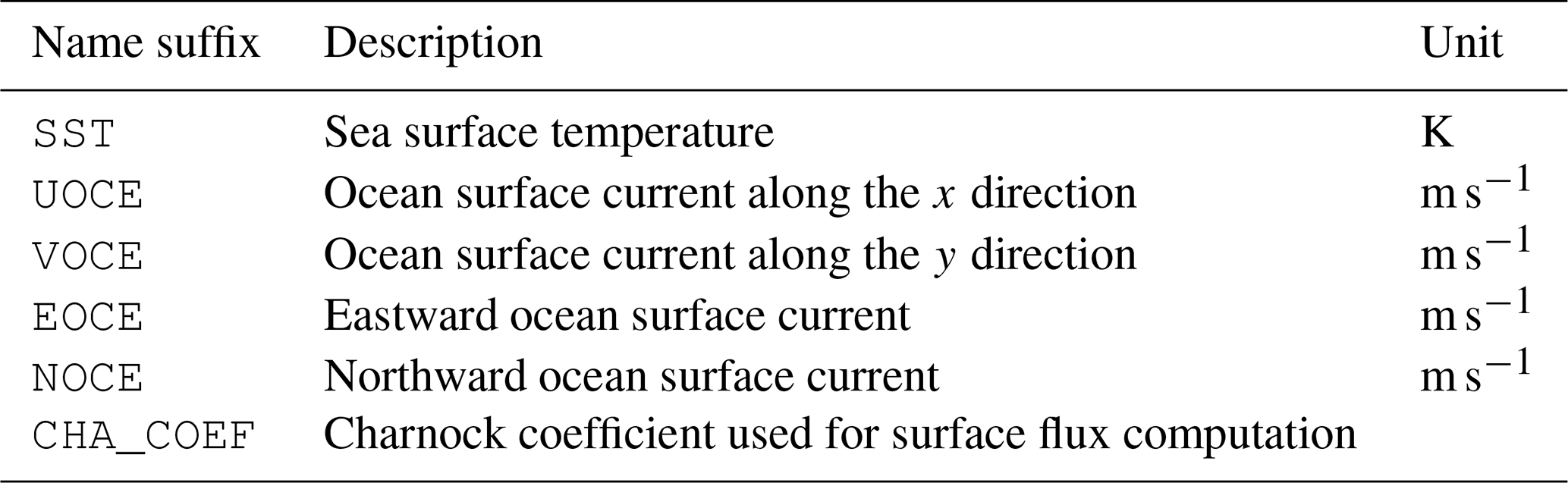
Table 4 List of the variables potentially sent in the current version of the coupling interface.

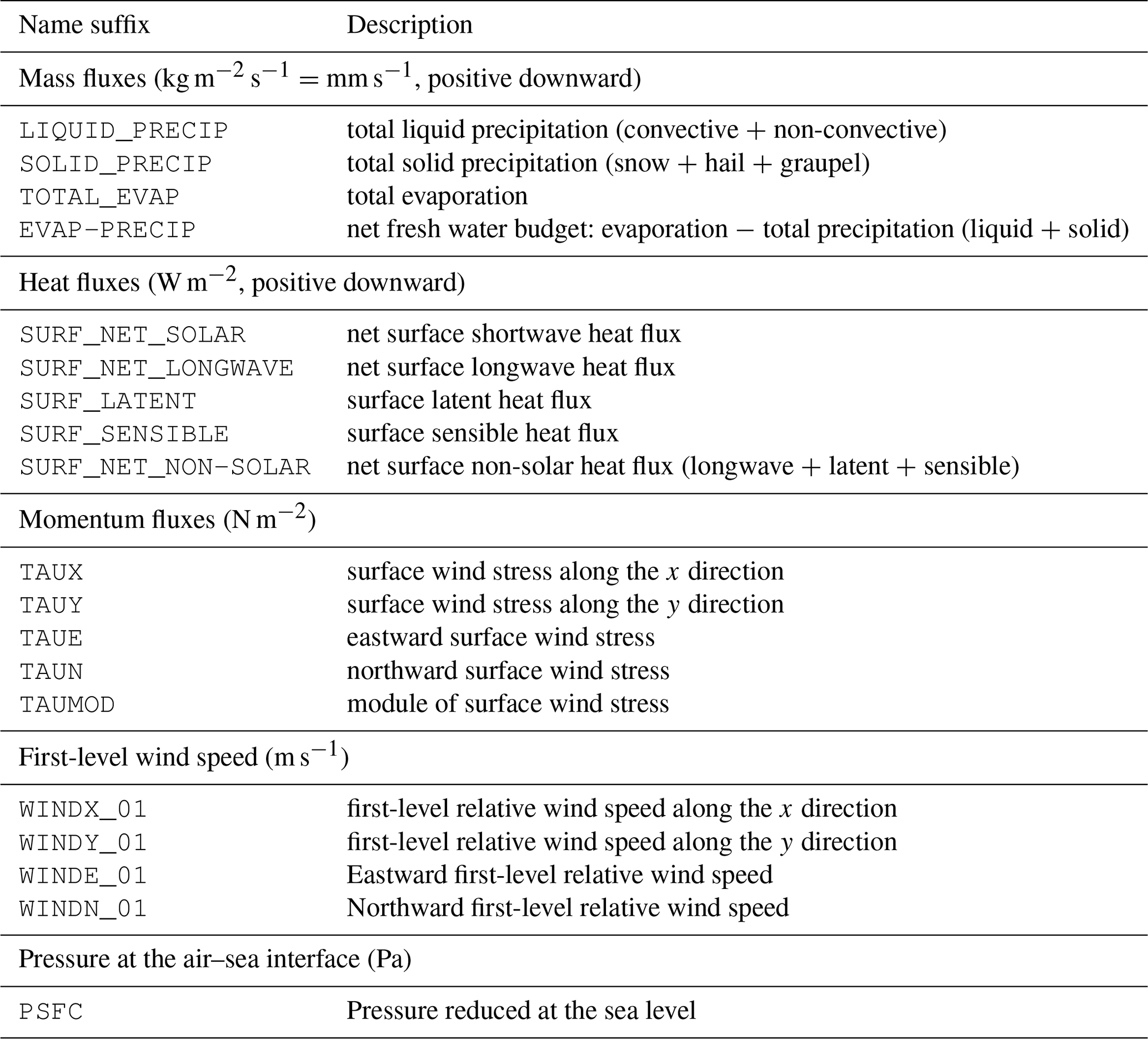
The variables potentially sent by WRF to the coupler are either directly available in WRF (already defined in WRF registry files) or are computed based on existing variables (defined in WRF registry) before being sent to the coupler. We typically compute net solar and non-solar heat fluxes, as well as the net freshwater flux. We additionally coded several options for the vector fields to send or receive as they may need to be rotated if the local orientation of the i and j directions of the WRF grid differs from that of the external domain to which they are coupled. We therefore provide the vector fields in a common geographic orientation (east and north components). An example of such treatment is available in the current code for the first-level wind speed (WINDE_01, WINDN_01), the surface wind stress (TAUE, TAUN), and the ocean surface currents (EOCE, NOCE). This work is done in the subroutine cpl_snd of frame/module_cpl.F.

As mentioned in Sect. 2.4.2, in the current version, all received variables are 2D surface fields used in phys/module_surface_driver.F and are treated in the subroutine cpl_rcv_sfcdrv. Adding other variables to be received is quite trivial as soon as we know how to use them in a different part of WRF code.

4 A multi-scale tool

After detailing the general structure of our coupling interface implementation in WRF, this section describes how we designed it in order to be (1) compatible with nested domains in WRF and/or in the models coupled with WRF, (2) as flexible as possible in its usage, and (3) easy to maintain and to adapt to any future application.

4.1 Coupling mask for received variables

Our coupling interface has been especially designed to be compatible with the nesting capability available in WRF and/or in external models coupled to WRF. We have introduced the concept of a coupling mask to meet our needs in terms of coupling interface. This coupling mask will be used, for example, when coupling an atmospheric domain whose geographical extent is greater than that of the ocean model. To do this, we use for the SST in WRF a blend of the SST received from the ocean model over the area common to both models and the SST read in wrflowinp_dxx over the part of the atmospheric domain not covered by the ocean model. The coupling mask will also be used when coupling an atmospheric domain with two nested oceanic grids. In this case, the SST of the two ocean grids will have to be combined to fulfill the WRF SST field.

4.1.1 Coupling mask definition

The coupling mask, called CPLMASK, is between 0 and 1, where 1 corresponds to coupled points and 0 to uncoupled points. Values between 0 and 1 can be used to merge coupled and uncoupled values as described in Sect. 4.1.2 and 4.1.3. This coupling mask is defined as a 3D array. Its third dimension, called num_ext_model_couple_dom, is the maximum number of external domains involved in the coupling. Note that in the wrfinput file, CPLMASK appears as a 4D array, with the third dimension called num_ext_model_couple_dom_stag and the fourth dimension called Time (that is always equal to 1). The third dimension must always exist even if we consider only one external domain in the coupling. In this case, num_ext_model_couple_dom is be equal to 1. CPLMASK is declared in the file Registry/Registry.EM_COMMON:

state real cplmask i{ ncpldom} j misc 1 z i0r
"CPLMASK" "COUPLING MASK (0:VALUE FROM
 SST UPDATE; 1:VALUE FROM COUPLED
OCEAN), vertical dim is number of
 external domains" ""

The dimension num_ext_model_couple_dom is declared in the file Registry/registry.dimspec:

dimspec ncpldom 2 namelist=num_ext_model_
 couple_dom z num_ext_model_couple_dom

The value of num_ext_model_couple_dom is defined in the domains section of the WRF namelist through the variable num_ext_model_couple_dom (equal to 1 by default). This namelist variable is also defined in the file Registry/Registry.EM_COMMON:

rconfig integer num_ext_model_couple_dom
 namelist,domains 1 1 - "number of
  external models
domains for coupling, used for the
 coupling mask" "" ""

As specified by i0r in the definition of CPLMASK in Registry/Registry.EM_COMMON, this variable is added in the main input and restart files of WRF domain number xx (wrfinput_dxx and wrfrst_dxx) and is by default set to 0 everywhere. CPLMASK must therefore be modified according to the coupled configuration requested by the user.

Here we give a simple example of how to modify CPLMASK using the land category for the ocean flag in the LU_INDEX variable of wrfinput_dxx. This example uses ncap2, one of the NCO operators, which are common tools to manipulate NetCDF files (Zender 2008).

# modify CPLMASK based on the LU_INDEX
 used for ocean
(here 17)

ncap2 -O -s "CPLMASK(0,0,:,:)=LU_INDEX == 17"
wrfinput_d01 wrfinput_d01

As each WRF domain (parent and children) has its own wrfinput_dxx input files, CPLMASK may differ for each WRF domain. In the current implementation, as CPLMASK is defined in wrfinput_dxx, it is fixed in time. If needed, we could imagine defining it differently, either through a time-varying auxiliary input file (e.g., wrflowinp_dxx) or even by means of a physical criterion on a given variable, e.g., the sea ice cover.

4.1.2 Coupling mask use

To favor a simple and generic management of exchanged variables and coupling mask, all variables received by a WRF domain are defined over the entire domain independently of the geometry of the external domain which send them. In other words, the coupler must interpolate the data from the external domain to the WRF domain without leaving any undefined point. CPLMASK(:,:,nn), where nn is the index of the external domain of interest, is then used as a multiplying factor applied to each variable received from the external domain nn.

It must be equal to 1 only if the field received from domain nn is considered and 0 if the field from domain nn is not considered. Fractional values, between 0 and 1, of CPLMASK can be used as weight factors to merge data received from several external domains (different external model grids and/or input data prescribed in the wrflowinp_dxx file). The mask value used to consider the data prescribed in wrflowinp_dxx is equal to 1 minus the sum of the CPLMASKs of all the external domains involved in the coupling. The data received from the coupler and read in wrflowinp_dxx is then merged by adding together all the weighted data:

field = sum(CPLMASK(:,:,nn)*field_rcv_nn)
+ (1-sum(CPLMASK(:,:,nn))*field_from_wrflowinp

For example, in an ocean–atmosphere configuration where SST for WRF domain 1 is received from two ocean model domains and from the wrflowinp_d01 file, the merged SST would be

SST(:,:) = CPLMASK(:,:,1) *
 SST_received_from_external_domain_01

+ CPLMASK(:,:,2) *
  SST_received_from_external_domain_02

+ (1 - (CPLMASK(:,:,1) + CPLMASK(:,:,2))
  * SST_from_wrflowinput

As the coupling frequency of a given variable can be different for each external domain and can also be different from the forcing interval of the wrflowinp_dxx file, it is necessary to store in memory each received or read field. This allows for an update to the consolidated value by re-merging the fields as soon as one of them has been newly received from the coupler or read in wrflowinp_dxx. All variables received from the coupler are thus stored in a structure, named srcv, which is internal to frame/module_cpl_oasis3.F. They are, in this way, available for a merge at any time step even if the timing does not correspond to the coupling date with a given external domain. Variables read in wrflowinp_dxx are stored in memory by calling the subroutine cpl_store_input from frame/module_cpl.F. Today, this routine deals only with the SST, which is duplicated in the new variable SST_INPUT (declared in Registry/Registry.EM) as soon as it is read in wrflowinp_dxx. It would be trivial to do the same for the other variables received by WRF (such as UOCE, VOCE and CHA_COEF). Today, for the sake of simplicity, these variables have a default constant value that will be used when the sum of external coupled domain CPLMASKs is not equal to 1 (see Sect. 4.1.3). This default value is defined in the cpl_rcv_sfcdrv subroutine of frame/module_cpl.F. We use 0.0185 for CHA_COEF. If not specified, this default value is equal to 0.0 (case of UOCE and VOCE).

4.1.3 An example: ocean–atmosphere coupling with nests on both sides

This example illustrates the coupling between WRF and an ocean model. Both WRF and the ocean model include a two-way nested domain. There are therefore two domains in WRF (d01 and d02) that will be coupled to two external domains (d01 and d02) coming from the same executable, here named OCE. In order to represent the different cases possibly found in such a coupling, we define the models' domains with different extents as follows (see Fig. 18a):

• WRF d01 (45° S–20° N, 110–50° W, resolution of $\mathrm{1}/\mathrm{4}$°, largest orange rectangle),

• WRF d02 (40° S–3°  N, 95–55° W, resolution of $\mathrm{1}/\mathrm{12}$°, smallest orange rectangle),

• OCE d01 (43° S–10° N, 100–68.5° W, resolution of $\mathrm{1}/\mathrm{12}$°, largest cyan rectangle),

• OCE d02 (37–5° S, 90–69.5° W, resolution of $\mathrm{1}/\mathrm{36}$°, smallest cyan rectangle).

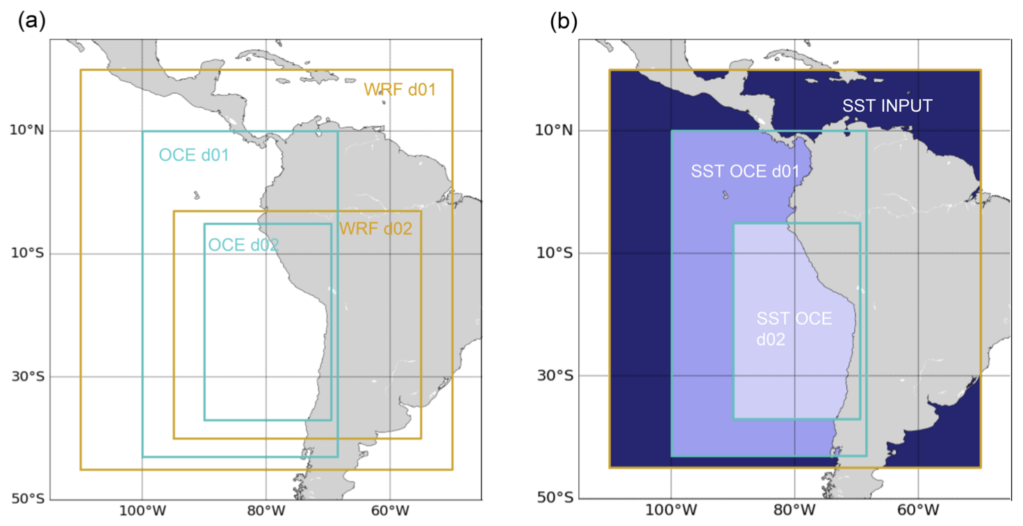
Figure 18 Example of a configuration with two nested domains in the atmospheric and ocean models with different extents: (a) extents of the WRF domains (WRF d01 and WRF d02, orange boxes) and of the ocean domains (OCE d01 and OCE d02, cyan boxes) and (b) available sea surface temperatures (SSTs) from the wrflowinp file (identified as SST INPUT, dark blue) and the two ocean domain SSTs (identified as SST OCE d01 in blue and SST OCE d02 in light blue).

Let us consider the SST as an example of a received field. As WRF parent domain d01 encompasses a larger region than both ocean domains, WRF d01 will use SST_INPUT from the wrflowinp_d01 file over places not covered by the ocean parent domain and over WRF “water points” excluded from the ocean model land–sea mask: e.g., lake Maracaibo in Venezuela or the small part of the Atlantic Ocean off the shore of Costa Rica, Panama and Colombia (dark-blue part in Fig. 18b). As OCE d01 ($\mathrm{1}/\mathrm{12}$°) is updated by the OCE d02 ($\mathrm{1}/\mathrm{36}$°) and has a finer resolution than WRF d01 ($\mathrm{1}/\mathrm{4}$°), we consider it is sufficient to send the OCE SSTs to WRF d01 only from OCE d01. The coupled mask used by WRF d01 is thus set as follows:

• The first level, CPLMASK(:,:,1), is set to 1 over the ocean part covered by OCE d01 with a 10-point wide linear transition to 0 close to the OCE d01 limits and is set to 0 elsewhere (Fig. 19a). This ensures a smooth transition between the prescribed SST_INPUT out of the OCE d01 limits and the received SST inside the OCE d01 limits.

• The second level, CPLMASK(:,:,2), is 0 everywhere as we decided to not send the SST of OCE d02 to WRF d01 (Fig. 19b).

WRF child domain d02 is almost fully covered by the ocean domains except for its southeastern corner over the Atlantic Ocean and non-ocean waterbodies such as lakes and rivers/deltas, where it will thus use SST_INPUT. Over the Pacific area, both OCE d01 SST (in dark blue) and OCE d02 SST (in light blue) will be used (Fig. 19b). The coupled mask used by WRF d02 is thus set up as follows:

• The first level, CPLMASK(:,:,1), is set to 1 over the ocean part covered by OCE d01 (Fig. 19c).

• The second level, CPLMASK(:,:,2), is set to 1 over the ocean part covered by OCE d02 (Fig. 19d).

Input files for running real coupled applications and the OASIS namcouple file, which is used to set the exchanges between WRF and the OCE model in such a complex example, are provided in Appendix B.

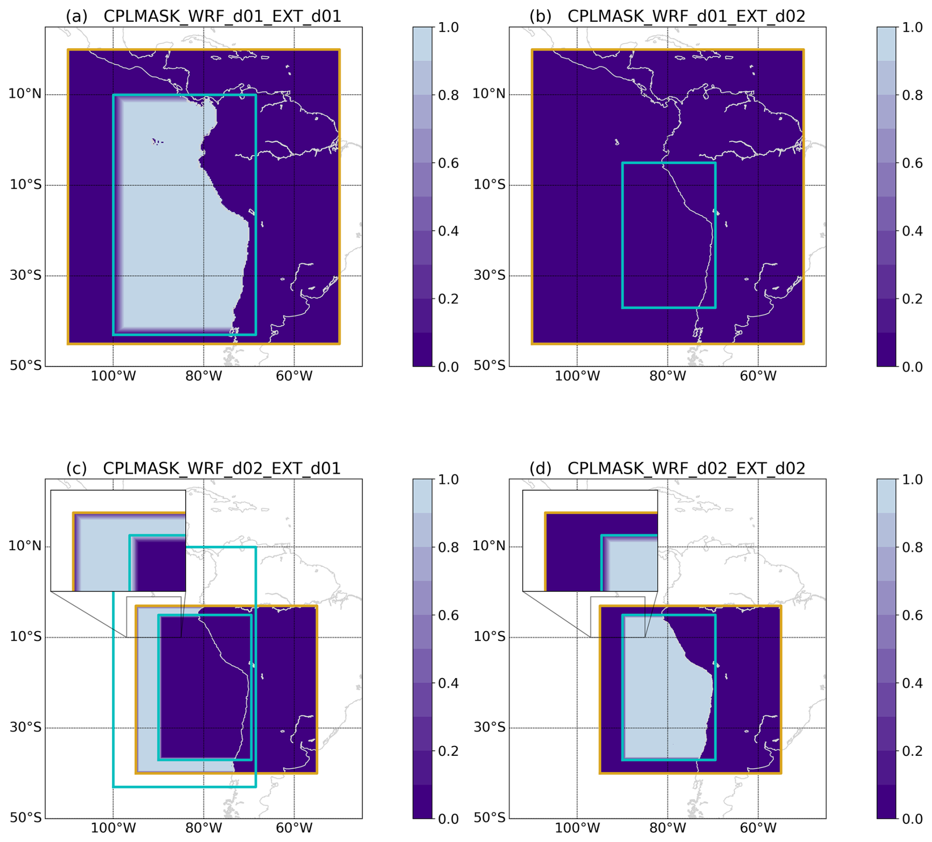
Figure 19 Coupling masks for the example configuration presented in Fig. 18: (a) CPLMASK for WRF d01 from external domain 1 (OCE d01), (b) CPLMASK for WRF d01 from external domain 2 (set to 0 as we do not consider the input from OCE d02 for this domain), (c) CPLMASK for WRF d02 from external domain 1 (OCE d01), (d) CPLMASK for WRF d02 from external domain 2 (OCE d02). A value of 1.0 corresponds to fully coupled; 0.0 corresponds to not coupled; and, for example, 0.5 to half coupled.

4.2 Deeper in the external domain concept and use

Other types of coupling could be performed with this coupling interface. We could, for example, imagine coupling WRF to an ensemble of N ocean models running in parallel to smooth out some part of the ocean stochastic variability. In this case, the WRF executable would be coupled to N ocean executables, each one sending its own SST. In such a case, we would have N external domains, and the weights used in each of the N coupling masks would simply be $\mathrm{1}/N$: CPLMASK(:,:,1:N) = 1./N. All the ocean models would receive the very same atmospheric forcing.

Other unconventional coupled experiment can be performed by extending the concept of external domains, which are not necessarily connected to a model or an executable. In a more general view, the definition of the external domain used for sent variables even differs from the definition used for received variables.

When receiving data, the external domain can be assimilated to a single number (nn) used to identify a set of variables sharing the same coupling mask CPLMASK(:,:,nn). This means that all variables from the same external domain will be multiplied by the same CPLMASK(:,:,nn) once received by WRF. This definition usually applies to variables sent by the same domain (parent or child) of a model coupled to WRF, but other applications could be imagined.

One could decide to use different CPLMASKs for variables received from the same model. For example, if one wants to test if a specific area is key for the SST coupling, one could build a configuration where WRF is coupled to a unique ocean model sending SST, UOCE and VOCE and decide that (1) UOCE and VOCE are coupled everywhere, but (2) the SST is merged with SST_INPUT (read in wrflowinp_dxx) over some parts of WRF domain. We would, in this case, need two coupling masks and define two external domains even if we couple only with one external model: CPLMASK(:,:,1) for UOCE and VOCE and CPLMASK(:,:,2) with a user-defined geometry to merge SST and SST_INPUT where it is needed.

Conversely, one can also imagine using the same CPLMASK for variables received from different executables, implying a unique external domain definition. For example, we could imagine coupling WRF with two ocean models, one sending the SST the other sending UOCE and VOCE, and decide to use the same CPLMASK for these three variables even if they are sent by different models.

When sending data, the external domain can also be assimilated to a single number, but, in this case, it is used to ensure the uniqueness of the name used to identify each variable sent by WRF (see naming conventions in the next section). This functionality is typically used when sending the same variable to different external domains as, for example, each domain could require its specific interpolation. For example, when sending the total net surface solar radiation (GSW) to the parent and child domains of an ocean model or to an ocean model and a land surface model, a different number must be associated with each sending request of the same variable, and each receiving domain (belonging to the same model or not) must be identified with a different external domain number.

Even if we detailed here the different possibilities offered by the concept of an external domain and a coupling mask, we suggest, whenever it is possible, to associate each external domain number to the one of the external model domains for more clarity when setting up a coupled configuration. Following this idea, we defined only a unique namelist parameter num_ext_model_couple_dom to fix the maximum number of external domains to be considered in a simulation independently of sending or receiving action. Note that this parameter still offers the possibility of using different numbers of external domains for sending or receiving data. Note also that num_ext_model_couple_dom must be smaller than or equal to the parameter max_extdomains defined in frame/module_driver_constants.F. If needed, its default value (5) can be increased to any size.

5 Conclusion and discussion

The present paper presents the implementation and use of a non-intrusive, multi-scale, and flexible coupling interface in WRF. This interface is designed with the following baselines: (1) it is structured with a two-level design through two new modules – a general coupling module and a coupler-specific module; (2) the exchange of variables, coupling frequency, and possible time and grid transformation are controlled thanks to an external text file; and (3) a coupling mask is used to determine and potentially merge fields that can be received from various external sources (e.g., different models, domains with different resolutions or wrflowinput file).

Presently, the only implemented coupler using this interface is OASIS3-MCT, but the structure is designed to allow adding more choices as the main coupling steps are thought to be generic to any coupler. The two-level interface provides a structure for users who wish to add their own coupler to the interface by developing the equivalent of frame/module_cpl_oasis3.F for their coupler. For OASIS3-MCT, all the required functionalities are likely already coded in frame/module_cpl_oasis3.F, which should not require further modifications. This allows users to modify the coupling interface without going into the intricacies of OASIS3-MCT.

We implemented in this coupling interface the exchanges of 2D surface fields for coupling with ocean and wave models. The current list of variables potentially sent or received is detailed in Sect. 3.3 and can be summarized as the momentum, heat and freshwater fluxes, as well as the adjusted sea level pressure for the possibly sent variables, and the SST, currents and Charnock coefficient as the possibly received variables. Our developed interface accounts for the vector transformation eventually needed in the case of rotated grids. We also explained how coupling with surface currents or the Charnock coefficient needs some modifications to the boundary layer and surface schemes to fully integrate the associated feedback. In WRF, several options exist for such schemes, and only part of them have been modified to account for the coupling – namely, the YSU and MYNN boundary layer schemes and the revised MM5 Monin–Obukhov surface scheme.

The coupling interface described here presently involves only 2D arrays from the surface module, but it is completely open, and it is possible to implement other kind of coupling, for example, with another (global) atmospheric model, or with a chemistry model that would require coupling 3D fields from other parts of the model. Adapting the current coupling interface would just require modifying the sending/receiving routines of frame/module_cpl.F to be compatible with 3D arrays and adding calls in the WRF routines requesting the exchanged fields as we did in the surface driver with the subroutine cpl_rcv_sfcdrv (see, for example, Briant et al., 2017). OASIS limitations would however impose using the same mask and the same the number/frequency of exchanged variables for every vertical level.

OASIS3-MCT requires that all the coupling specifications (i.e., which variables are sent/received to/from which domain) are defined before any coupling exchange of variables from the parent grid. This constraint has two consequences. First, as explained in Sect. 2.4.1, the coupling interface works with a maximum of one level of nested grids. However, this limitation is relatively easy to circumvent. To do so, one would have to move the loop defining the child grids (DO WHILE ( nests_to_open )…) from integrate to wrf_init. As this loop must be called recursively to initiate all domains, the simplest modification would be to put this loop in a small recursive subroutine called at the end of wrf_init. Thereby, all nested grid definition would be done at once during the initialization phase, before the first time step of the parent grid in agreement with OASIS3-MCT requirements. This modification of the WRF code would however prevent initiating and ceasing the child grids at any time, a feature required by some users. Its clean implementation would therefore need additional modifications of the code to reconcile all WRF usages. We thought that there is not enough need for multi-level nesting in couple mode to implement this work and decided to keep the code as closest as possible to its original version.

Another similar partial solution is to allow having more than one nest but to couple only the parent grid and the first nest. This can easily be achieved by limiting the number of WRF domains involved in the coupling to two, a modification concerning only three lines of code.

In frame/module_cpl_oasis3.F, replace

IF ( pgrid%id == pgrid%max_dom ) CALL
cpl_oasis_enddef()

by

IF ( pgrid%id == MIN(2,pgrid%max_dom) ) CALL
cpl_oasis_enddef()

In frame/module_integrate.F, replace

IF (coupler_on) CALL cpl_defdomain(
new_nest )

by

IF ( coupler_on .AND. new_nest%id <=
MIN(2, new_nest%max_dom) ) CALL
cpl_defdomain( new_nest )

and replace

IF (coupler_on) CALL cpl_defdomain(
new_nest )

by

IF ( coupler_on .AND. new_nest%id <=
MIN(2, new_nest%max_dom) ) CALL
cpl_defdomain( new_nest )

Second, the grid is defined only once at the initialization stage, which prevents the use of the moving nest ability of WRF as the model grid is moving over time when this option is activated. A partial solution is simply to couple only the WRF parent static domain with an ocean or wave model. The moving grids are not directly involved in the coupling interface but do play an indirect role through the feedbacks (1) of the fields computed in the WRF moving nest domain(s) to WRF parent domain and (2) of the coupled fields received in the WRF parent domain and provided to the moving nest(s) (e.g., SST). This strategy has the advantage of using atmospheric fields calculated at high resolution in the nests and interpolated on the WRF d01 domain to feed the ocean or wave model and of considering the feedback of surface conditions provided by the coupler in the evolution of the parent and moving nests while maintaining the coupling interface simple. To do so, one must use two-way moving nest(s) and allow the interpolation of WRF d01 received SST field into the moving nest, so that coupled SST is accounted for in the moving nests. This requires to slightly modify the Registry/Registry.EM as

state real SST ij misc 1 - i01245rh05d=
 (interp_mask_ field:lu_index,iswater)f
  =(p2c) "SST"
"SEA SURFACE TEMPERATURE" "K"

Finally, note that WRF adaptive time step was not tested. It probably does not work as, for example, the coupling time must correspond to a multiple of the time step. We also have not tested this coupling interface in OpenMP. Although OASIS exchange routines can be used on an OpenMP-compatible model, assuming that the coupling library has also been compiled with the OpenMP option, the coupling variables should necessarily be collected on the main thread before being supplied as arguments.

Appendix A: Shell script used to build OASIS3-MCT files, grids.nc, masks.nc and areas.nc

At the following link, we provide a shell script that can be used to build the OASIS3-MCT files called grids.nc, masks.nc and areas.nc from the WPS geogrid file: https://github.com/massonseb/WRF/blob/GMD_wrf_coupling/tools/create_wrf_grids_masks_areas.sh (last access: 20 August 2024). Note that this shell script uses NCO operators (Zender, 2008).

Appendix B: Examples of a namcouple and other input files

At the following link, we provide, as an example, the namcouple file used in the coupled model described in Sect. 4.1.3: https://github.com/massonseb/WRF/blob/GMD_wrf_coupling/run/namcouple_example (last access: 6 September 2024).

Input files for running real applications are also provided on two Zenodo repositories. The first one is an example of a coupling between WRF, WAVEWATCH III and CROCO (https://doi.org/10.5281/zenodo.14235410, Jullien, 2024a), and the second one is an example of a WRF-CROCO coupling with a two-way nested domain in CROCO (https://doi.org/10.5281/zenodo.14235450, Jullien, 2024b).