Monitoring and benchmarking Earth system model simulations with ESMValTool v2.12.0

Earth system models (ESMs) are important tools to improve our understanding of present-day climate and to project climate change under different plausible future scenarios. Thus, ESMs are continuously improved and extended, resulting in more complex models. Particularly during the model development phase, it is important to continuously monitor how well the historical climate is reproduced and to systematically analyze, evaluate, understand, and document possible shortcomings. Hence, putting model biases relative to observations or, for example, a well-characterized pre-industrial control run, into the context of deviations shown by other state-of-the-art models greatly helps to assess which biases need to be addressed with higher priority. Here, we introduce the new capability of the open-source community-developed Earth System Model Evaluation Tool (ESMValTool) to monitor running simulations or benchmark existing simulations with observations in the context of results from the Coupled Model Intercomparison Project (CMIP). To benchmark model output, ESMValTool calculates metrics such as the root-mean-square error, the Pearson correlation coefficient, or the earth mover's distance relative to reference datasets. This is directly compared to the same metric calculated for an ensemble of models such as the one provided by Phase 6 of the CMIP (CMIP6), which provides a statistical measure for the range of values that can be considered typical of state-of-the-art ESMs. Results are displayed in different types of plots, such as map plots or time series, with different techniques such as stippling (maps) or shading (time series) used to visualize the typical range of values for a given metric from the model ensemble used for comparison. While the examples shown here focus on atmospheric variables, the new functionality can be applied to any other ESM component such as land, ocean, sea ice, or land ice. Automatic downloading of CMIP results from the Earth System Grid Federation (ESGF) makes application of ESMValTool for benchmarking of individual model simulations, for example, in preparation of Phase 7 of the CMIP (CMIP7), easy and very user-friendly.

1 Introduction

Earth system models (ESMs) are complex numerical representations of the Earth system, including not only interactions between the physical components, such as atmospheric, oceanic, land, and sea ice dynamics, but also climate-relevant chemical and biological processes. Over the past years, ESMs have become essential tools to better understand the human impact on the climate system and to project future climate change under different emission scenarios.

Therefore, ESMs are continuously being developed and improved, with new processes added and existing processes described in more detail. As with any model development activity, a thorough evaluation of new model results is a fundamental prerequisite to assess model performance, and thus model suitability, for a given scientific application (fitness for purpose). However, evaluating ESMs has become quite complex, as there is a growing multitude of relevant parameters from different Earth system components that typically require a team of scientists with different expertise to fully assess all details. Furthermore, evaluation of some parameters, such as biogeochemical components, might suffer from a lack of global observations that are suitable for a comparison with the model results, as such parameters are very hard to obtain.

One possibility to quickly assess deviations from the observations present in a new model simulation is to put them into perspective by comparing the biases with those obtained from a large number of other state-of-the-art ESMs. For this purpose, for example, results from Phase 5 and 6 of the Coupled Model Intercomparison (CMIP) (Eyring et al., 2016; Taylor et al., 2012) can be used to get an overview of which biases can be considered “acceptable for now” and which would need more attention and more detailed analysis and comparison with observations. The same approach can be used to monitor running model simulations to identify significant problems early on. A number of software tools for model evaluation have been developed over recent years. Examples include the PCMDI Metrics Package (PMP; Lee et al., 2024), the International Land Model Benchmarking (ILAMB) system (Collier et al., 2018), and the Earth System Model Evaluation Tool (ESMValTool; Righi et al., 2020). In this article, we demonstrate the new capability of ESMValTool to obtain a broad overview by benchmarking a given model simulation with CMIP results using different relevant diagnostics such as climatologies, seasonal and diurnal cycles, or geographical distributions. The examples are meant as a starting point and can be easily extended and applied to different components of the Earth system.

2 Methods

2.1 Earth System Model Evaluation Tool

The Earth System Model Evaluation Tool (ESMValTool) is an open-source community-developed diagnostics and performance metrics tool for the evaluation and analysis of Earth system models with Earth observations (Righi et al., 2020; Eyring et al., 2020; Lauer et al., 2020; Weigel et al., 2021). ESMValTool has been developed into a well-tested and well-documented tool that facilitates analysis across different Earth system components (e.g., atmosphere, ocean, land, and sea ice). ESMValTool can be run on any Unix-style operating system that supports the installation of cross-platform package managers such as Mamba (recommended) or Conda. The package manager is used to install all dependencies including NetCDF or programming languages such as R or Julia. There are no external compilers or system libraries needed. Datasets available on the Earth System Grid Federation (ESGF) can be optionally downloaded automatically; for observationally based datasets not available on ESGF, ESMValTool provides a collection of scripts with downloading and processing instructions to obtain such observational and reanalysis datasets.

While originally designed to facilitate a comprehensive and rapid evaluation of models participating in the CMIP, the tool can now also be used to analyze some output from regional models, a large variety of gridded observational data, and reanalysis datasets. Recent improvements include the possibility to read and process operational output of selected models produced by running a model through its standard workflow, without the requirement to apply further post-processing steps as well as the strongly improved capability to handle unstructured grids (Schlund et al., 2023).

ESMValTool allows for consistent processing of all model and observational datasets, such as regridding them to common grids, the masking of land/sea and missing values, and vertical interpolation. This allows for a fair comparison of all diagnostics and metrics calculated for individual models with each other. With the recently added features of being able to specify model datasets with wildcards and the automatic download of datasets from the ESGF, ESMValTool is well suited to provide the context for comparing model deviations from observations with each other in an easy and convenient way. This allows one to check a large set of parameters and provides the flexibility to extend existing benchmarking “recipes” easily. Recipes are ESMValTool configuration files that define all input data, preprocessing steps, and diagnostics or metrics to be applied. For example, in order to request the first ensemble member (r1i1p1f1) from all available historical runs of Phase 6 of the CMIP (CMIP6), the dataset section in a recipe would be as follows:

datasets:
- project: CMIP6
exp: historical
dataset: `*'
institute: `*'
ensemble: `r1i1p1f1'
grid: `*'.

More information for users and developers of ESMValTool, including how to write own recipes, can be found in the documentation available at https://docs.esmvaltool.org (last access: 1 January 2025). For new users, there is a tutorial available at https://tutorial.esmvaltool.org (last access: 1 January 2025).

The output of ESMValTool typically consists of plots (e.g., png or pdf), NetCDF file(s), provenance record(s), log files, and an HTML file summarizing the output in a browsable way. All examples shown in this publication can be reproduced with ESMValTool version 2.12.0 using the recipes “recipe_lauer25gmd_fig*.yml” available on Zenodo (https://doi.org/10.5281/zenodo.11198444, Jöckel et al., 2025).

2.2 Available metrics

For the purpose of assessing the general performance of a new model simulation and to quickly identify potential problems that require more attention, a number of metrics, such as the bias or root-mean-square error, are available that can be applied over 1D or multiple-dimension coordinates of a dataset. These dimensions include longitude, latitude, and time; for parameters that are vertically resolved, they also include a vertical coordinate, such as pressure or altitude. For example, consider two 3D datasets (model and reference) with time, latitude, and longitude dimensions. If a metric is applied over the time dimension, the result is a 2D map with latitude and longitude dimensions; if a metric is applied over the horizontal latitude and longitude dimensions, the result is a 1D time series with a time dimension.

The metrics have been implemented as generic preprocessing functions that are newly available in v2.12.0. In contrast to previously available diagnostic-specific implementations of such metrics, the preprocessing functions can be applied to ensembles of models and arbitrary variables and dimensions, providing the flexibility needed for the new benchmarking and monitoring capabilities of ESMValTool described here. For all metrics, an unweighted and weighted version exists. In the latter case, each point (in time and/or space) that enters the metric calculation is weighted with a factor w_i (details on the calculations are given in the corresponding sections below). The time weights are calculated from the input data using the bounds provided for each time step (“time_bnds” variable) to obtain the length of the time interval. The individual time steps of the input data are then weighted using the lengths of the time intervals. As provision of time bounds is mandatory for a dataset to be compliant with the CMOR (Climate Model Output Rewriter) standard, this can be done for all input data. This method accounts for different calendars and years (e.g., leap year versus non-leap years). For area-weighting, the grid cell area sizes are used. In the case of regular grids, area sizes can be either given as a supplementary variable specified in the ESMValTool recipe (typically the “areacella” or “areacello” CMOR variables) or calculated from the input data. In the case of irregular grids, the grid cell areas must be provided as a supplementary variable.

While the weighted version is the preferred option for most use cases, an unweighted option is available for cases in which weighing with the grid box area might distort the results. Examples of such cases include extracting individual model grid cells containing a measurement station and giving the same weight to each station, independent of the model grid box area. If a metric is calculated over time and geographical coordinates, the weights are calculated as the product of the above. Weights are normalized, i.e., $\sum _{i=\mathrm{1}}^N{w}_i=\mathrm{1}$ (where N represents the number of data points).

The following sections give an overview of the metrics that are available.

2.2.1 Bias and relative bias

The “BIAS” metric calculates the difference between a given dataset X and a reference dataset R (e.g., observations) as follows:

$$\begin{array}{}\text{(1)}& \mathrm{BIAS}=X-R.\end{array}$$

The relative bias is obtained by dividing by the reference dataset R as follows:

$$\begin{array}{}\text{(2)}& {\mathrm{BIAS}}_{\mathrm{rel}}={\displaystyle \frac{X-R}{R}}.\end{array}$$

In order to avoid spurious values as a result of very small values of R, an optional threshold to mask values close to zero in the denominator can be provided.

2.2.2 Root-mean-square error

The average root-mean-square error (RMSE) between a dataset X and a reference dataset R is calculated as follows:

$$\begin{array}{}\text{(3)}& {\mathrm{RMSE}}_{\mathrm{weighted}}=\sqrt{\sum _{i=\mathrm{1}}^N{w}_i{\left(X_i-R_i\right)}^{\mathrm{2}}}.\end{array}$$

Here, N gives the number of coordinate values over all dimensions over which the metric is applied and w_i represents the normalized weights. A smaller RMSE corresponds to better performance. More information on the weights is given at the beginning of Sect. 2.2.

2.2.3 Pearson correlation coefficient

The Pearson correlation coefficient (r) measures the linear correlation between two datasets and is defined as the ratio between the covariance of two variables and the product of their standard deviations:

$$\begin{array}{}\text{(4)}& r_{\mathrm{weighted}}={\displaystyle \frac{\sum _{i=\mathrm{1}}^N\left[w_i\left(X_i-\stackrel{\mathrm{‾}}{X}\right)\left(R_i-\stackrel{\mathrm{‾}}{R}\right)\right]}{\sqrt{\sum _{i=\mathrm{1}}^N\left(w_i{\left(X_i-\stackrel{\mathrm{‾}}{X}\right)}^{\mathrm{2}}\right)}\sqrt{\sum _{i=\mathrm{1}}^N\left(w_i{\left(R_i-\stackrel{\mathrm{‾}}{R}\right)}^{\mathrm{2}}\right)}}}.\end{array}$$

Here, $\stackrel{\mathrm{‾}}{X}$ and $\stackrel{\mathrm{‾}}{R}$ denote the average of the dataset X and R, respectively, over the selected dimension coordinate, and w_i represents the normalized weights. A larger r corresponds to better performance. Again, more information on these weights is given in the beginning of Sect. 2.2.

2.2.4 Earth mover's distance

The earth mover's distance (EMD), also known as the first-order Wasserstein metric W₁, is a metric to measure the similarity between two probability distributions of datasets X and R (Rubner et al., 2000). It can be understood as the minimum amount of work needed to transform one distribution into the other. This concept is often explained using the analogy of moving piles of earth, where the EMD quantifies the cost required to move the earth from one pile to another, with the cost being proportional to the amount of earth moved and the distance that it has traveled. Recently, the EMD has gained more attention for applications in climate science, such as an evaluation of the performance of climate models (e.g., Vissio et al., 2020). Here, we implement the EMD in a similar fashion to Vissio et al. (2020) but for 1D distributions (i.e., to one variable at a time) and focusing on the W₁ metric (i.e., the EMD) only. First, we use data binning over all dimensions over which the EMD is calculated to get the normalized probability mass functions p_x(x_i) and p_r(r_i) with n bins. Here, x_i and r_i are the bin centers of X and R, respectively. The bins range from the minimum to the maximum value of the data calculated over both the dataset and reference dataset; thus, x_i=r_i for all i. For the weighted EMD, each value only contributes its associated weight w to the bin count; for the unweighted EMD, each value contributes an equal weight. Details on the weighting is given at the beginning of Sect. 2.2. With these probability mass functions, the EMD can be expressed as follows:

$$\begin{array}{}\text{(5)}& \mathrm{EMD}=\stackrel{\inf }{\mathit{\gamma }\mathit{ϵ}\mathrm{\Pi }\left(p_x,p_r\right)}\sum _{i,j}^n{\mathit{\gamma }}_{ij}\left|x_i-r_j\right|.\end{array}$$

Here, Π(p_xp_r) denotes the set of all joint probability distributions γ with marginals p_x and p_r. The sum describes the aforementioned transportation cost, which is proportional to the “amount of earth moved” (characterized by γ) and the “distance the earth has traveled” (characterized by absolute differences in the bin centers). The γ that minimizes this transportation cost is called the “optimal transport matrix”. In practice, for our simple 1D case, the EMD can be calculated analytically with the cumulative distributions of x and r (see Remark 2.30 in Peyré and Cuturi, 2019, for details). The EMD is not sensitive to the number of bins n and provides robust results even with small values of n (Vissio et al., 2020; Vissio and Lucarini, 2018). The default value of equally sized bins in ESMValTool is n=100, but that can be changed by the user if desired. As the EMD is a true metric in the mathematical sense, smaller values of EMD correspond to better performance.

2.3 Datasets

In the following, all observationally based datasets used as a reference for the examples below are briefly described alongside the model data. For more details, we refer to the references given in the individual subsections.

2.3.1 Reference data

In the following, all reference datasets used are listed in alphabetical order and briefly described. We would like to note that we do not advocate that the datasets used in the examples are particularly suitable for specific applications or might be preferable over alternative options.

CERES-EBAF

The Clouds and the Earth's Radiant Energy System (CERES) Energy Balanced and Filled (EBAF) Ed4.2 dataset (Kato et al., 2018; Loeb et al., 2018) provides global monthly mean top-of-atmosphere (TOA) longwave (LW), shortwave (SW), and net radiative fluxes under clear-sky and all-sky conditions. CERES instruments are on board NASA's Terra and Aqua satellites. These are used to calculate the TOA longwave (lwcre) and shortwave (swcre) cloud radiative effect as differences between the TOA all-sky and clear-sky radiative fluxes. The dataset covers the time period from 2001 to 2022 on a global 1°×1° grid.

ERA5

ERA5 is the fifth-generation reanalysis of the European Centre for Medium-Range Weather Forecasts (ECMWF) (Hersbach et al., 2020), replacing the widely used ERA-Interim reanalysis (Dee et al., 2011). ERA5 uses a 4D variational (4D-Var) data assimilation scheme and Cycle 41r2 of the Integrated Forecasting System (IFS) (C3S, 2017). Here, we use ERA5 data served on the Copernicus Climate Change Service Climate Data Store (CDS) that are interpolated to a horizontal resolution of 0.25°×0.25° and, in the case of 3D variables, to 37 pressure levels ranging from 1000 hPa near the surface to 1 hPa (ECMWF, 2020).

GPCP-SG

The Global Precipitation Climatology Project (GPCP) is a community-based analysis of precipitation that covers the satellite era from 1979 to present. The data are produced by merging different data sources, including passive microwave-based rainfall retrievals from satellites (SSMI and SSMIS), infrared rainfall estimates from geostationary (GOES, Meteosat, GMS, and MTSat), polar-orbiting satellites (TOVS and AIRS), and surface rain gauges (Adler et al., 2003, 2018). Here, we use version 2.3 of GPCP-SG that provides monthly mean precipitation rates on a global 2.5°×2.5° grid from January 1979 to present. GPCP-SG is widely used as a reference dataset for precipitation (e.g., Bock et al., 2020; Eyring et al., 2021; Hassler and Lauer, 2021; Nützel et al., 2024).

HadCRUT5

The Met Office Hadley Centre–Climatic Research Unit global surface temperature dataset HadCRUT5 contains monthly averaged near-surface temperature anomalies on a regular 5°×5° grid from 1850 to near the present. HadCRUT5 combines sea surface temperature measurements from ships and buoys and near-surface air temperature measurements from weather stations over land. There are two versions of HadCRUT5 available, a version representing temperature anomalies for the measurement locations (“non-infilled”) and a second version for which a statistical method has been applied for a more complete data coverage (“analysis”) (Morice et al., 2021). Here, we use the ensemble mean of the analysis version of the dataset. HadCRUT5 is widely used as a reference dataset for near-surface temperature (e.g., Eyring et al., 2021; Uribe et al., 2022).

HadISST

The Hadley Centre Sea Ice and Sea Surface Temperature dataset (HadISST) provides a combination of monthly globally complete fields of SST and sea ice concentration on a 1°×1° grid from 1870 to date. The SST data are taken from the Met Office Marine Data Bank (MDB) with input from the International Comprehensive Ocean–Atmosphere Data Set (ICOADS) where no data from the MDB are available (Rayner et al., 2003). For the example shown below, we use HadISST version 1.1 monthly average sea surface temperature.

ISCCP-FH

The International Satellite Cloud Climatology Project radiative flux profile dataset (ISCCP-FH; Zhang and Rossow, 2023) provides radiative flux profiles with a global resolution of 1°×1° at 3-hourly and monthly intervals. ISCCP-FH data that are available over the time period from July 1983 through June 2017 are based on ISCCP H-series products derived from different geostationary and polar-orbiting satellite imagers (Young et al., 2018). Here, we use the monthly mean TOA clear-sky and all-sky radiative fluxes to calculate the shortwave and longwave cloud radiative effects for comparison with the models.

2.3.2 Model data

CMIP6

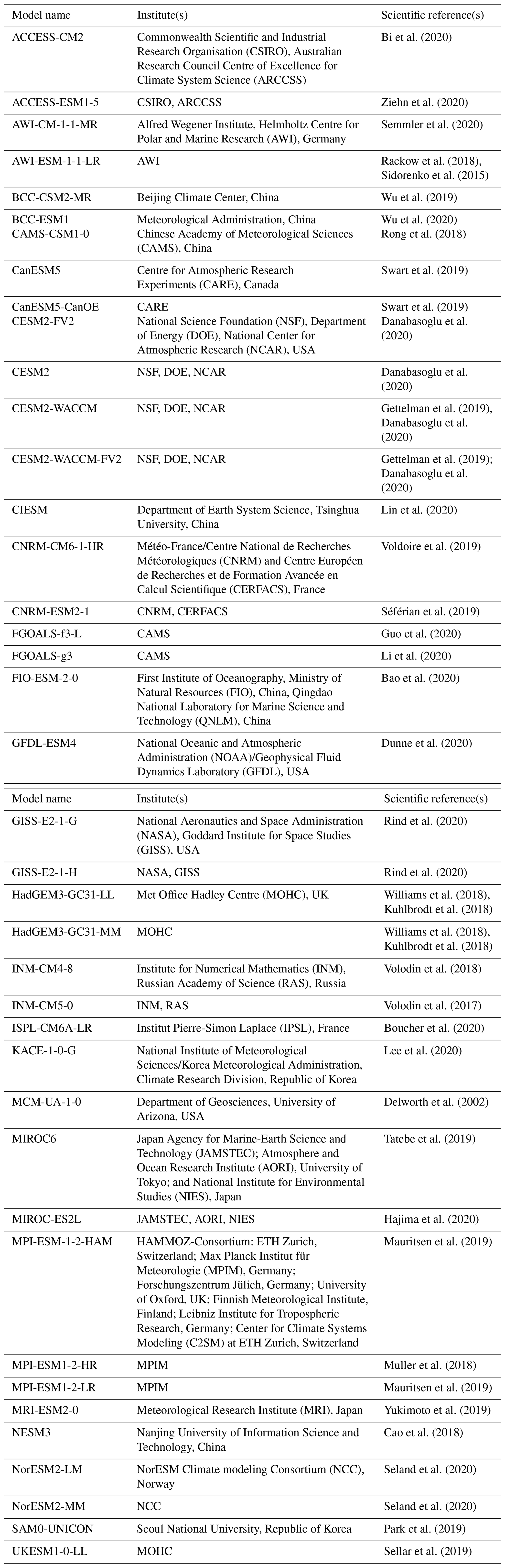
In this study, we use data from models participating in the latest phase of the CMIP (CMIP6; Eyring et al., 2016) to put model deviations from observations into the context of current ESMs. For this, we use results from the “historical” simulations, for which forcings due to natural causes, such as volcanic eruptions and solar variability, and human factors, such as CO₂ and concentrations or land use, were prescribed for the time period from 1850 to 2014. For the examples shown in this article, we use only one ensemble member (typically the first member “r1i1p1f1”) per model, as the inter-model spread is typically much larger than the inter-model spread given by different ensemble members from the same model (e.g., Lauer et al., 2023). Table 1 provides an overview of the CMIP6 models used.

Table 1 List of CMIP6 models providing data from the historical simulation that are compared with an example simulation from the EMAC model (see below) and put into the context of current ESMs. If more than one ensemble member is available, only the first ensemble member (typically “r1i1p1f1”) is used.

EMAC

The ECHAM/MESSy Atmospheric Chemistry (EMAC) model is a chemistry/climate model (Jöckel et al., 2010) that has been widely used for various studies in atmospheric sciences, including tropospheric and stratospheric ozone (e.g., Dietmüller et al., 2021; Mertens et al., 2021), the climate impact of contrails and emissions from aviation (e.g., Frömming et al., 2021; Matthes et al., 2021), and the effects of transport on the atmosphere and climate (e.g., Hendricks et al., 2018; Righi et al., 2015). EMAC uses the second version of the Modular Earth Submodel System (MESSy2) to link submodels for various physical and chemical processes to the host model. Here, the fifth generation of the European Centre Hamburg general circulation model (ECHAM5; Roeckner et al., 2006) is used as the host model.

In this study, we use an EMAC simulation with deliberately erroneous prescribed sea surface temperatures (SSTs) to showcase the application of the new ESMValTool features to monitor and benchmark model simulations during the model development phase with results from established global climate models. While a comparison of results from coupled historical CMIP6 simulations with an AMIP (Atmospheric Model Intercomparison Project)-style simulation in which SSTs and sea ice concentrations are prescribed from observations is, of course, not completely fair for a real model benchmarking or monitoring of a simulation, this approach allows us to showcase the new ESMValTool features with a simulation in which something goes wrong after a few simulation years. We would like to stress that the examples in the following are not meant to assess the performance of EMAC but, rather, to illustrate the new capabilities of ESMValTool with an easy-to-perform and easy-to-understand test simulation only. Likewise, using historical simulations from CMIP6 models for the comparison is an arbitrary choice and is done only for the purpose of illustrating the examples. Hence, the SST fields are set to zonally averaged monthly values of the observed global average SST after the first 5 years of model simulation (see Fig. 1). Such an error does not necessarily show up in time series of global mean near-surface temperature, but it can be identified when using other metrics. The approach of a single model simulation with an error introduced after 5 years allows us illustrate a case in which a problem occurs during the runtime of a model (see Sect. 3.1) and, at the same time, provide two datasets with and without a problem from the same model for comparison by splitting the simulation into two 5-year periods (Sect. 3.2–3.6). Again, we would like to stress that this is meant as an example to illustrate the new capabilities of ESMValTool, rather than to analyze or evaluate the EMAC simulation used.

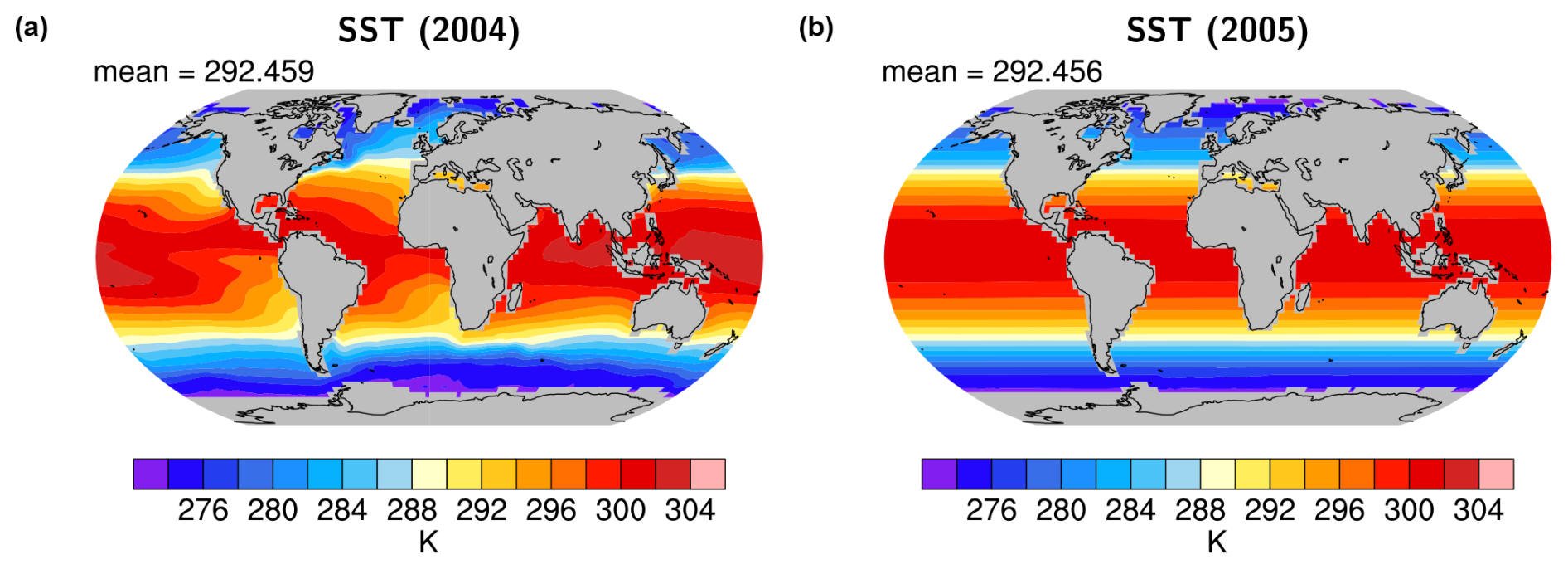
Figure 1 Annual mean of the prescribed sea surface temperatures (SSTs) for the EMAC simulation (a) before (year 2004) and (b) after (year 2005) the deliberately introduced “error”.

3 Monitoring and benchmarking of ESM simulations

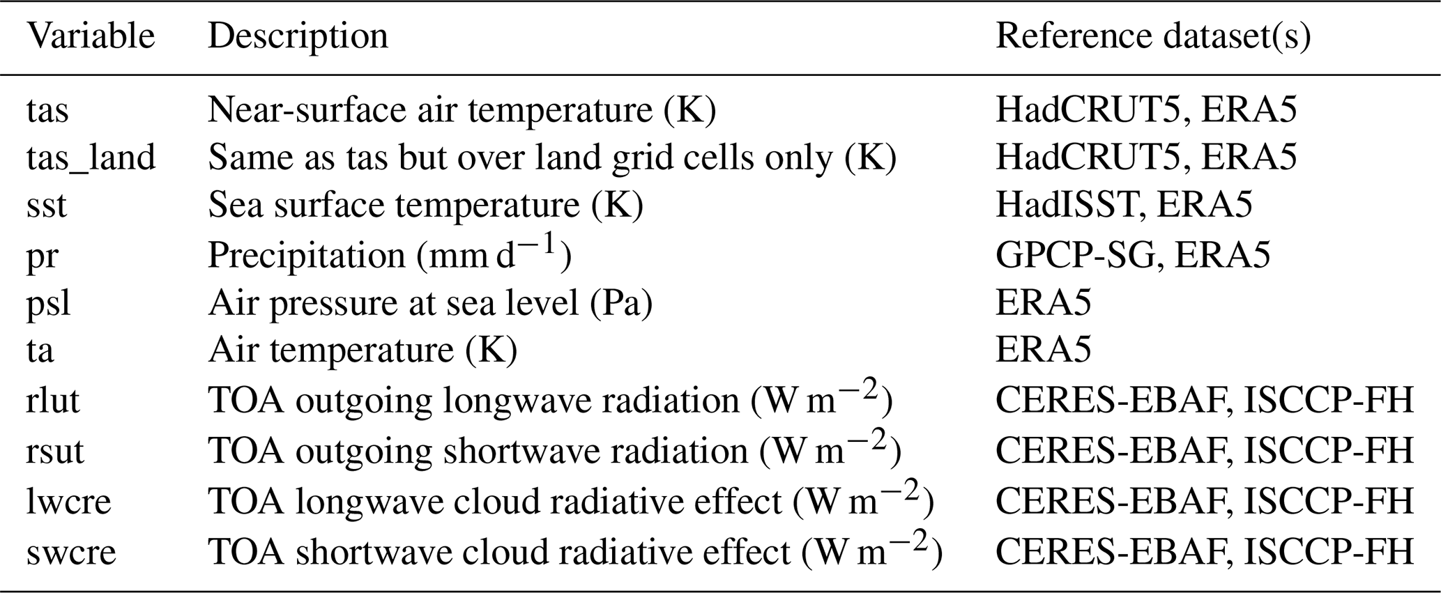
In the following, we show examples of how the new ESMValTool capabilities can be used to monitor and benchmark model simulations to detect problems during runtime and to assess whether the performance of a model simulation is within the range of what could be expected from current state-of-the-art ESMs (here CMIP6). The variables and reference datasets used in the examples are listed in Table 2. We would like to note that the new ESMValTool functionalities shown in the following are not limited to atmospheric quantities and can be applied to any ESM component, such as ocean, sea ice, and land ice. If no suitable observationally based reference dataset is available, a well-characterized reference model simulation can also be used to assess a simulation.

Table 2 Variables and reference datasets used.

3.1 Time series

Time series of climate-relevant quantities or their anomalies relative to a given reference period averaged over a specific region or the entire globe are a common approach to evaluate model results with one or several reference datasets (e.g., Bock et al., 2020; Yazdandoost et al., 2021; Wang et al., 2023). As an example, Fig. 2a shows a time series of global average anomalies in near-surface temperature. In addition to the EMAC model results (red line) and the observational reference data from HadCRUT5 (black line), the CMIP6 results (Table 1) are also shown (thin gray lines). The figure shows that the first 5 years of the EMAC simulation are at the high end of the CMIP6 results, with the temperature anomalies frequently exceeding the 90th percentile of the CMIP6 results. At the beginning of the year 2005, there is the sudden temperature drop when the deliberate error in the SST fields is introduced, resulting in the EMAC simulation being at the low end of the CMIP6 range, with temperature anomalies frequently being below the CMIP6 10th percentile. Figure 2b shows a time series of the global average (area-weighted) root-mean-square errors in simulated near-surface temperature from EMAC (red line). The 10th and 90th percentile range of the RMSE values from the individual CMIP6 models is shown as light-blue shading. The “error” in the geographical distribution of the sea surface temperatures introduced in 2005 is not obvious in this time series, as the performance of this EMAC simulation is within the range of what could be expected from a coupled CMIP6 model. This shows that monitoring of model simulations typically requires the assessment of several variables.

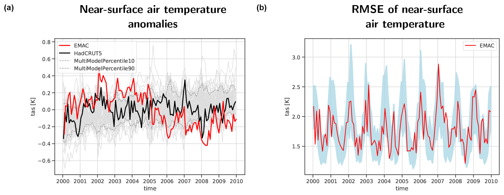
Figure 2 (a) Time series from 2000 through 2009 of global average monthly mean temperature anomalies (reference period 2000–2009) of the near-surface temperature (in K) from a simulation of EMAC (red) and the reference dataset HadCRUT5 (black). The thin gray lines show 43 individual CMIP6 models used for comparison, while the dashed gray lines show the 10th and 90th percentiles of these CMIP6 models. Panel (b) is the same as panel (a) but for the area-weighted RMSE of the near-surface air temperature. The light-blue shading shows the range of the 10th to 90th percentiles of the RMSE values from the ensemble of 43 CMIP6 models used for comparison.

3.2 Diurnal and seasonal cycle

A further commonly used metric for model evaluation is the comparison of the seasonal cycle of a specific variable, calculated for the whole globe or, again, for a pre-defined region. Figure 3a shows the multiyear global mean seasonal cycle of the near-surface air temperature for a suite of CMIP6 models, the HadCRUT5 observations, and the specifically created EMAC simulation that has been described in Sect. 2.3.2. The CMIP6 model simulations and the HadCRUT5 data are averaged over the time period from 2000 to 2009, whereas the EMAC simulation is split into the two 5-year periods without and with the erroneous SSTs, 2000–2004 (red line) and 2005–2009 (dark-blue line), respectively. Similar to Fig. 2a, Fig. 3a also indicates the 10th and 90th percentile range with dashed gray lines. Both 5-year means of the EMAC simulation are well within the CMIP6 10th and 90th percentile range throughout the whole year, but the EMAC simulation period with the correct SSTs is slightly closer to the HadCRUT5 data than the simulation period with the erroneous SSTs. While this is positively noted, it is not an inherent clear indication that a problem occurred with the latter 5-year period of the EMAC simulation. Figure 3b then shows the area-weighted RMSE values for the global mean seasonal cycle of near-surface air temperature. The blue shading depicts the 10th to 90th percentile range of the CMIP6 models used for the comparison. The earlier 5-year period of the EMAC simulation (2000–2004, red line) is below the blue shaded area in most months, meaning that, with correct SST fields, the example EMAC simulation can reproduce the seasonal cycle of near-surface temperature better than most CMIP6 models (a smaller RMSE represents better performance). With the erroneous SSTs, however, the RMSE values for the annual cycle become larger, which means that the agreement of the seasonal cycle of near-surface air temperature with the reference dataset decreased for that period of the EMAC simulation. The values are still located within the blue shaded area, but agreement is not as good as that for the earlier period (red line). Again, this metric alone would not allow the clear detection of a faulty simulation, but it would be clear that, in “normal” simulations, EMAC's performance is clearly better than most CMIP6 models when looking at the RMSE of near-surface air temperature, and a clear decrease in performance could be an indicator that there might be problem with a new simulation.

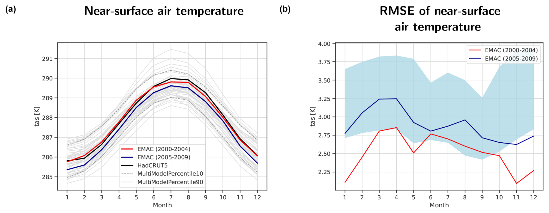
Figure 3 (a) Multiyear global mean of the seasonal cycle of near-surface air temperature (in K) from a simulation of EMAC averaged over the time periods from 2000 to 2004 (red) and from 2005 to 2009 (dark blue) and the reference dataset HadCRUT5 (2000–2009; black). The thin gray lines show 43 individual CMIP6 models (2000–2009) used for comparison, while the dashed gray lines show the 10th and 90th percentiles of these CMIP6 models. Panel (b) is the same as panel (a) but for the area-weighted RMSE of the near-surface temperature. The light-blue shading shows the range of the 10th to 90th percentiles of the RMSE values from the ensemble of 43 CMIP6 models used for comparison.

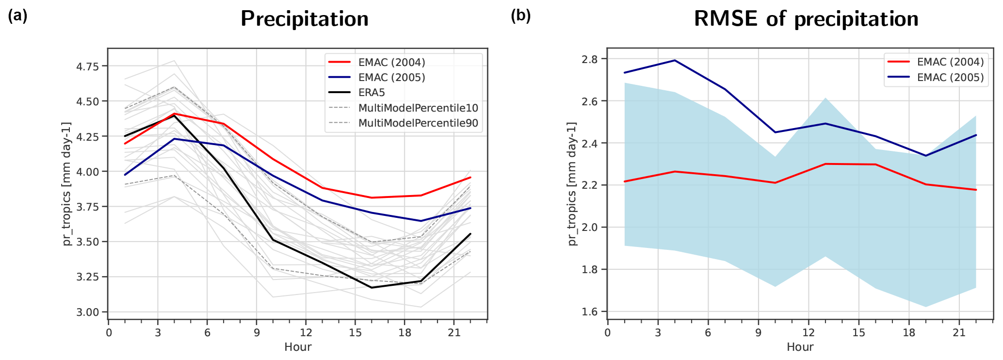
Figure 4 Annual mean diurnal cycle of precipitation averaged over the tropical ocean (ocean grid cells in the latitude belt from 30° S to 30° N) from a simulation of EMAC averaged over the year 2004 (red) and over 2005 (dark blue) compared with ERA5 data (2004–2005; black). The thin gray lines show 22 individual CMIP6 models used for comparison (2004–2005), while the dashed gray lines show the 10th and 90th percentiles of these CMIP6 models. Panel (b) is the same as panel (a) but for the area-weighted RMSE of precipitation. The light-blue shading shows the range of the 10th to 90th percentiles of the RMSE values from the ensemble of 22 CMIP6 models used for comparison.

A further capability implemented in ESMValTool is to intercompare the diurnal cycle of a variable, for example, precipitation (see Fig. 4). The basic structure of the graphs in Fig. 4 is identical to Fig. 3 regarding the shown EMAC simulation, the CMIP6 simulations, and their spread; however, the example results show the precipitation averaged only over the tropical ocean, instead of a global mean, and averaged over only 2 years (2004–2005). ERA5 has been used as the reference dataset. Both years of the EMAC simulation show a reduced amplitude of the average diurnal cycle of precipitation over the tropical ocean compared with ERA5 and most of the CMIP6 ensemble (Fig. 4a), with 2004 (from the “correct” period) being even further away from the reference compared with 2005 (from the erroneous period). Figure 4b shows the RMSE of the diurnal cycle of precipitation over the tropical ocean. The blue shaded region again indicates the 10th to 90th percentile range of the CMIP6 models. The year 2004 of the EMAC simulation is fully enclosed by the CMIP6 percentile range, whereas 2005 is above the CMIP6 percentile range for most hours of the day. This reversal of which EMAC simulation year performs better compared with ERA5 suggests that some kind of error compensation takes place when calculating the mean values (Fig. 4a), whereas this is not the case when calculating the RMSE value at each grid cell for a given time of the day and then averaging afterwards (Fig. 4b). Similar to the metric shown in Fig. 3, the comparison of the diurnal cycle of precipitation alone might not be able to correctly identify erroneous simulations, but this metric could give an indication that something might not be correct with a new simulation if it is possible to compare it to a “baseline” simulation of the same model that has been labeled as correct.

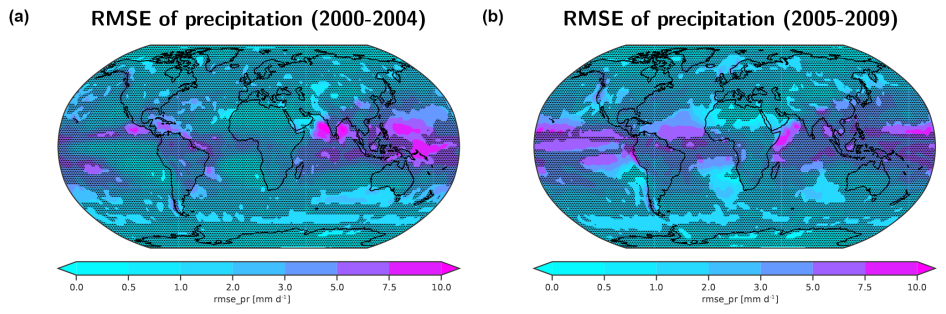
Figure 5 The 5-year annual mean area-weighted RMSE of the precipitation rate (in mm d⁻¹) from a simulation of EMAC compared with GPCP-SG data. Panel (a) shows the average over the time period from 2000 to 2004, whereas panel (b) presents the average over the time period from 2005 to 2009. The stippled areas mask grid cells where the RMSE is smaller than the 90th percentile of RMSE values from an ensemble of 39 CMIP6 models.

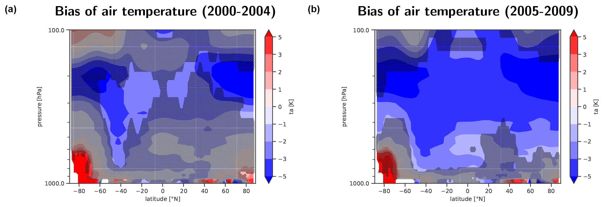
Figure 6 The 5-year annual mean bias of the zonally averaged temperature (in K) from a historical simulation of the EMAC model compared with ERA5 reanalysis data. Panel (a) shows the average over the time period from 2000 to 2004, whereas panel (b) present the average over the time period from 2005 to 2009. The stippled areas mask grid cells where the absolute bias (|BIAS|) is smaller than the maximum of the absolute 10th (|p10|) and the absolute 90th (|p90|) percentiles from an ensemble of 38 CMIP6 models, i.e., $\left|\mathrm{BIAS}\right|\le \max \left(\right|\mathrm{p}\mathrm{10}|,|\mathrm{p}\mathrm{90}\left|\right)$.

3.3 Geographical distribution

Figure 5 shows an example of how the RMSE of the time series of monthly mean precipitation at each grid cell from a given simulation can be compared with the range of RMSE values from the CMIP6 models. As a reference, GPCP-SG data are used (Sect. 2.3.1). The stippled grid cells denote areas in which the RMSE value of the given simulation is below the 90th percentile of RMSE values from the CMIP6 models. This threshold can be set depending on what is considered “OK” during model development or model benchmarking, allowing one to focus on the non-stippled areas showing larger deviations. Figure 5a shows the RMSE of the precipitation time series of the EMAC simulation for the period from 2000 to 2004. In this figure, non-stippled areas are mainly found in the tropical eastern Pacific and Indian Ocean, highlighting (1) the regions that show larger RMSE values than most of the CMIP6 models and that might need further investigation during model development or (2) the regions that perform worse than what could be expected from a state-of-the-art model. As a result of the deliberately introduced error in the geographical SST distribution in 2005, these areas are much larger in the second half (2005–2009) of the EMAC simulation (see Fig. 5b) and now cover most of the tropical oceans. When applied to the monitoring of a running simulation, this increase in areas performing less well than the majority of CMIP6 models can be a first indication of problems related to deep convection, which requires further investigation.

3.4 Zonal averages

For 3D variables, such as air temperature, a comparison of zonally averaged fields with reference data is an easy and common way to evaluate a model simulation. For this, the bias or relative bias can be used as a measure of how well the model simulation reproduces the reference data. In Fig. 6, the bias of the EMAC example simulation compared with ERA5 data for the zonally averaged 3D air temperature is shown. Here, the stippling indicates that the absolute value of the bias |BIAS| is smaller than the maximum of the absolute 10th and the absolute 90th percentiles, |p10| and |p90|, respectively, of the bias values from the CMIP6 ensemble for this grid cell. By using the criteria $\left|\mathrm{BIAS}\right|\le \max \left(\right|\mathrm{p}\mathrm{10}|,|\mathrm{p}\mathrm{90}\left|\right)$, positive and negative bias values are given the same importance when assessing the model performance. Depending on the aim of the model development and the percentiles selected for this comparison, all non-stippled bias values outside of this range can be regarded as below-par performance and might require further investigation and possibly continued model improvements or model tuning. When monitoring a running simulation, the strong increase in the grid cells that are marked as below-average performance between the first (Fig. 6a) and the second simulation time period (Fig. 6b) is a first hint that there might be an unexpected problem in the simulation that occurred during runtime.

3.5 Box plots

The summary plots for different variables (as shown in Fig. 7) offer a quick initial overview of model performance. This can either be used as a starting point for a more in-depth evaluation of individual variables/climate parameters with observations or as one possible summary of overall model performance. For every diagnostic field considered, model performance is compared to one reference dataset (see Table 2, first dataset), and the quality of the simulation is summarized using a single number, such as the RMSE (Fig. 7a and b), Pearson's correlation coefficient (Fig. 7c and d), or EMD (Fig. 7e and f) computed over the time-averaged global maps.

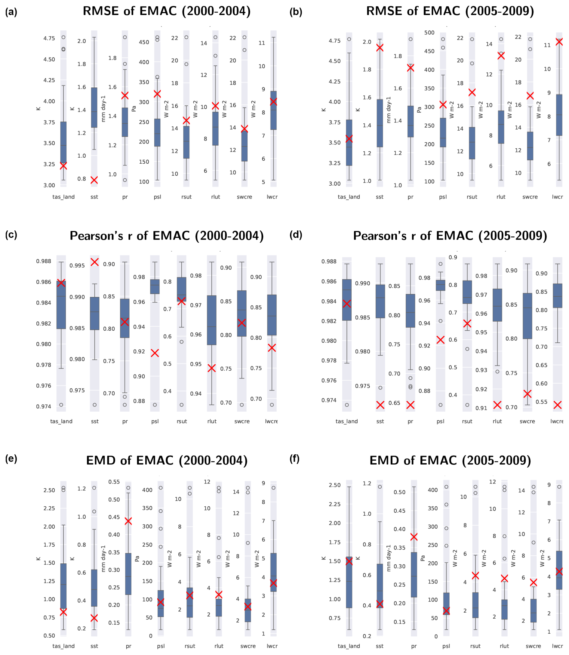
Figure 7 (a, b) The global area-weighted RMSE (smaller is better), (c, d) weighted Pearson's correlation coefficient (higher is better), and (e, f) weighted earth mover's distance (smaller is better) of the geographical pattern of 5-year means of different variables from a simulation of EMAC (red cross) in comparison to the CMIP6 ensemble (box plot). Panels (a), (c), and (e) show the results for the time period from 2000 to 2004, whereas panels (b), (d), and (f) present the results for the period from 2005 to 2009. Reference datasets for calculating the three metrics are as follows: near-surface temperature (tas) – HadCRUT5; surface temperature (ts) – HadISST; precipitation (pr) – GPCP-SG; air pressure at sea level (psl) – ERA5; and shortwave (rsut) and longwave (rlut) radiative fluxes at TOA and shortwave (swcre) and longwave (lwcre) cloud radiative effects – CERES-EBAF. Each box indicates the range from the first quartile to the third quartile, the vertical lines show the median, and the whiskers present the minimum and maximum values, excluding the outliers. Outliers are defined as being outside 1.5 times the interquartile range.

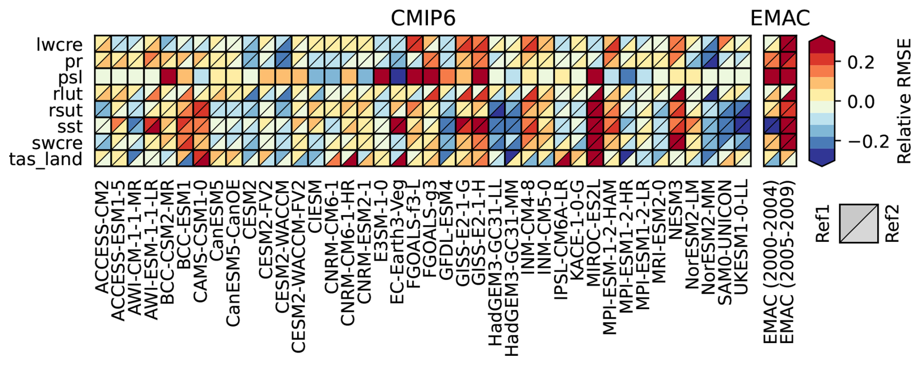
Figure 8 Portrait diagram showing the relative space–time root-mean-square error (RMSE) calculated from the seasonal cycle of the datasets. The seasonal cycle is averaged over the years from 2000 to 2009 (CMIP6 models) and over the time periods from 2000 to 2004 and from 2005 to 2009 for the EMAC simulation. The figure shows the relative performance, with blue shading indicating better performance and red shading indicating worse performance than the median RMSE of all models. The lower right triangle shows the relative RMSE with respect to the reference dataset (Ref1), whereas the upper left triangle shows the relative RMSE with respect to an alternative reference dataset (Ref2). Using the RMSE as a metric (as shown) gives a portrait diagram similar to Gleckler et al. (2008). Other metrics are available.

By simultaneously assessing a number of different performance indices, the general model improvements can then be quantified and compared with the CMIP6 ensemble. In our example EMAC simulation, the SSTs are prescribed; thus, we see significantly better performance with respect to the SST compared with the CMIP ensemble of coupled (historical) simulations, especially regarding the RMSE (Fig. 7a) and Pearson's correlation coefficient (Fig. 7c). For the other variables, the EMAC example often shows slightly worse performance than the 75th percentile of the CMIP6 models, but it mostly still lies within the range of the CMIP6 models. This changes when we look at the second time period (Fig. 7b), for which we can see a significant decrease in model performance regarding the RMSE for all variables. Furthermore, it can be seen that the decrease in the performance in the second time period is most prominent for the SSTs, especially with respect to the RMSE and correlation pattern values (Fig. 7b and d). This is a clear hint that detailed diagnostics for this variable (e.g., see Fig. 2) would be helpful in order to quickly identify the error in the simulation.

3.6 Portrait diagram

Portrait diagrams (Gleckler et al., 2008) can be used to visualize model performance across different variables relative to one or multiple reference datasets. Unlike box plots, portrait diagrams show the performance of each model individually; thus, they provide a convenient way to benchmark each element in an ensemble of models. Figure 8 shows an example of a portrait diagram for the same set of variables as used in the box plots (see Fig. 7). The horizontal axis shows the different models (left: the CMIP6 models; right: the EMAC simulation for two different time periods), whereas the vertical axis presents the different variables. The colors correspond to the relative RMSE (relative to the median RMSE across all models) of the different models and variables: red corresponds to a higher RMSE (worse performance) and blue to a lower RMSE (better performance) than the median. For variables for which the box is split into two triangles, an alternative dataset is provided in the lower right triangle (see Table 2 for an overview of variables and reference datasets used). The effect of the deliberately introduced error in the EMAC simulation is clearly visible on the right side of the portrait diagram: as expected, the incorrect SST pattern starting in 2005 leads to a sharp decline in the relative RMSE in SST, from dark-blue colors (i.e., very good performance) in 2000–2004 to dark-red colors (i.e., very bad performance) in 2005–2009. However, the error is not only visible in the SST: across all variables, the later period (2005–2009) of the EMAC simulation shows a higher relative RMSE (i.e., worse performance) than the corresponding early period (2000–2004). In addition to the RMSE, the EMD or Pearson correlation coefficient metrics could also be used (see Sect. 2.2).

4 Summary and discussion

In this paper, we introduce the newly extended capability of the Earth System Model Evaluation Tool to benchmark and monitor climate model simulations across a wide range of different Earth system components. The new framework allows one to put common performance metrics calculated for a given model simulation into the context of results from an ensemble of state-of-the-art climate models, such as those participating in Phase 6 of the Coupled Model Intercomparison Project. Putting the performance of a model simulation into such a context allows one to quickly assess whether, for instance, the values obtained for metrics such as the bias or pattern correlation for a variable are within the typical range of model errors or might need further, more detailed investigation. This is particularly helpful during model development or when monitoring a simulation to identify possible problems early (during runtime), as this allows a large number of variables to be assessed without the need for detailed expert knowledge on each single quantity. This is also helpful when automatizing the monitoring of running simulations. For this, the numerical output of ESMValTool in the form of NetCDF files could be used to summarize the results from the different metrics with, for example, a dashboard displayed on a website showing a green, yellow, or red traffic light for each quantity tested depending on the results. The percentiles for the metric obtained from the model ensemble used for comparison can be employed as thresholds to flag quantities that are outside the range of typical model errors and, thus, in need of further inspection. A possible application for these new model benchmarking and monitoring capabilities of ESMValTool would be the assessment of new model simulations during the preparation phase for Phase 7 of the CMIP.

As shown in Sect. 3, particularly for model development, these metrics are most effective if there are already results from a well-tuned, well-understood baseline simulation of the same model available. When the results of this baseline simulation are known, the evaluation and benchmarking of a new simulation can be done quite effectively with a few simulation years, as the deviation from the baseline quickly become apparent for many relevant atmospheric variables. For the examples shown in this paper, for instance, we found that the use of 5 model years is usually sufficient for this kind of initial assessment.

The possibility to use wildcards in recipes when specifying the model datasets (available since ESMValTool version 2.8.0), which is employed to provide context for comparison in combination with the feature to download any data that are missing locally but that are available on the ESGF automatically (available since ESMValTool version 2.4.0), makes application of ESMValTool for model benchmarking and monitoring very easy and user-friendly. Examples of how to use the new capabilities of ESMValTool for benchmarking and monitoring include time series; seasonal and diurnal cycles; and map plots, box plots, and portrait diagrams for any 2D variable including individual levels or, for instance, zonal averages of 3D variables that can be shown as latitude–height plots.

The benchmarking and monitoring diagnostics introduced in this paper currently support bias and relative bias, Pearson's correlation coefficient, root-mean-square error, and earth mover's distance as metrics. All of these metrics can be calculated as unweighted or weighted metrics (e.g., by using the area size of the grid cells as weights for the latter). As all of these basic metrics are implemented in the form of a generic preprocessing function of ESMValTool, adding new metrics is straightforward, and new metrics can then be used by all diagnostics with little to no additional effort.