The Earth Science Box Modeling Toolkit (ESBMTK 0.14.0.11): a Python library for research and teaching

The Earth Science Box Modeling Toolkit (ESBMTK) is a Python library that streamlines the creation and analysis of box models in earth sciences. With its modular, object-oriented design, ESBMTK simplifies the study of systems such as the long-term carbon cycle or the impact of atmospheric CO₂ variations on ocean chemistry. By standardizing and clarifying how models are defined, the library enhances code readability and serves as a self-documenting tool, making it approachable for undergraduate students and efficient for researchers. ESBMTK automatically translates user-defined models into equations which are solved using established numerical libraries. It also includes built-in functionality for common tasks such as ocean–atmosphere gas exchange, marine carbonate chemistry, isotope effects, and perturbation scenarios. The library's core interface is stable, supported by comprehensive documentation, and available as open-source software through the pip and conda package management systems.

1 Introduction

Box modeling is a versatile tool to explore a variety of earth system processes. Modest hardware requirements facilitate its use for teaching or investigating problems that require long integration times. Prominent examples include, e.g., Harvardton-Bear type models for exploring aspects of the marine carbonate system (e.g., Broecker et al., 1999); the GEOCARBSULF model, which describes the evolution of the carbon, oxygen, and sulfur biogeochemical cycles over Phanerozoic times (Berner, 2006); or the LOSCAR model, which models the atmospheric and marine carbon system components and their C-isotope ratios (Zeebe, 2012). Even limiting the citations to a specific subject area like paleoceanography results in a long list of publications demonstrating the importance of box modeling (e.g., Sarmiento and Toggweiler, 1984; Tyrrell, 1999; Wallmann, 2003; Ridgwell, 2003; Tyrrell and Zeebe, 2004; Archer, 2005; Wortmann and Chernyavsky, 2007; Slingerland and Kump, 2011; Markovic et al., 2015; Bachan and Kump, 2015; Luo et al., 2016; Rennie et al., 2018; Yao et al., 2018; Boudreau et al., 2018, 2019; Shields and Mills, 2021; Mills et al., 2021; Paytan et al., 2021).

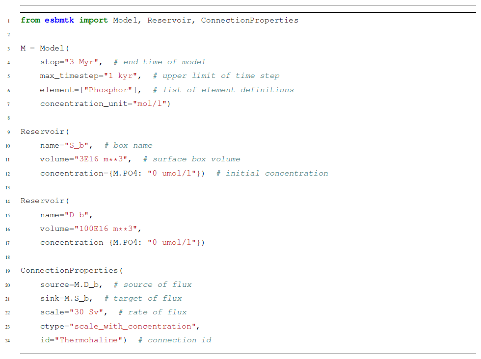
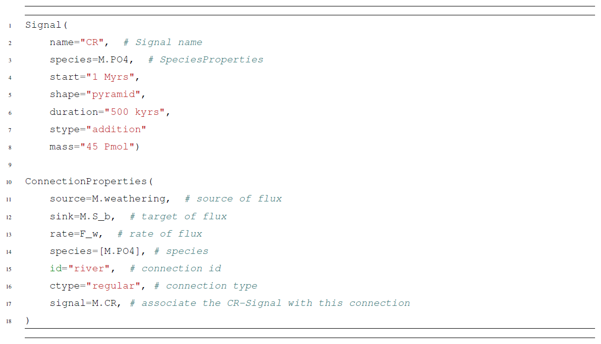
Listing 1 Code fragment showing how to import ESBMTK classes and create Reservoir objects (instances; see Fig. 1). The ConnectionProperties instance defines the relationship between Reservoir instances. In this case, it is a flux that depends on the volume of water and time in Sverdrup (1×10⁶ m² s⁻¹) and the concentrations of the species in the source Reservoir. Note that ESBMTK is unit aware and that the name of the ConnectionProperties instance is set implicitly.

Box models, unlike more complex earth system models, require minimal computational resources. This allows researchers to focus on specific aspects of the earth system, e.g., how carbonate sediment dissolution mitigates ocean acidification. However, many undergraduate and graduate earth science students lack proficiency in traditional coding languages and differential equation solving, which limits the use of box models in classroom settings. The simplicity and widespread adoption of Python, along with the availability of cloud-based computing environments like Jupyter Notebooks, have expanded coding accessibility beyond traditional audiences. Here, we introduce a Python library that separates model geometry (and processes) from the underlying numerical implementation and thus allows students (and researchers) to focus on the conceptual challenges, rather than mathematical theory. We successfully used this library in undergraduate and graduate teaching, as well as for ongoing research projects.

Our approach is best demonstrated by a simple example. Box models are formulated as a system of coupled ordinary differential equations (ODEs) that describe, e.g., the transfer of matter between Reservoir instances (boxes). To give a trivial example (following Glover et al., 2011), let us consider the concentration of phosphate in a two-box ocean. The concentration change in phosphate in the surface box is simply a function of the phosphate fluxes into and out of the box:

$$\begin{array}{}\text{(1)}& {\displaystyle \frac{\mathrm{d}{\left[{\mathrm{PO}}_{\mathrm{4}}\right]}_{\mathrm{S}}}{\mathrm{d}t}}={\displaystyle \frac{F_{\mathrm{w}}+F_{\mathrm{u}}-F_{\mathrm{d}}-F_{\mathrm{POP}}}{V_{\mathrm{S}}}},\end{array}$$

where F_w denotes the PO₄ weathering flux, F_u denotes the PO₄ upwelling flux, F_d denotes the PO₄ flux related to the thermohaline circulation, F_POP denotes the PO₄ uptake by primary production, and V_S denotes the volume of the surface box.

While conceptually simple, translating the above into computer code is often beyond the coding skills of many earth science students. Furthermore, with increasing model complexity, the reverse process, i.e., deriving the governing relationships from the program code, becomes considerably more difficult. The Earth Science Box Modeling Toolkit (ESBMTK) aims to address both problems by facilitating a declarative model definition that also serves as the model documentation. Modeling objects (instances in Python) are created by importing the respective ESBMTK classes which are then used to create, e.g., Reservoir objects (see e.g., Listing 1).

Class instances can then be combined to build a model, e.g., a Reservoir instance (say, for the surface ocean box), which can be connected to a second Reservoir instance (e.g., the deep-ocean box) via a connection instance that specifies their relationship (e.g., scale by concentration; see line 12 in Listing 1). This results in a hierarchical structure that, while verbose, explicitly encodes the model geometry and the relationships between the respective model objects (see Fig. 1).

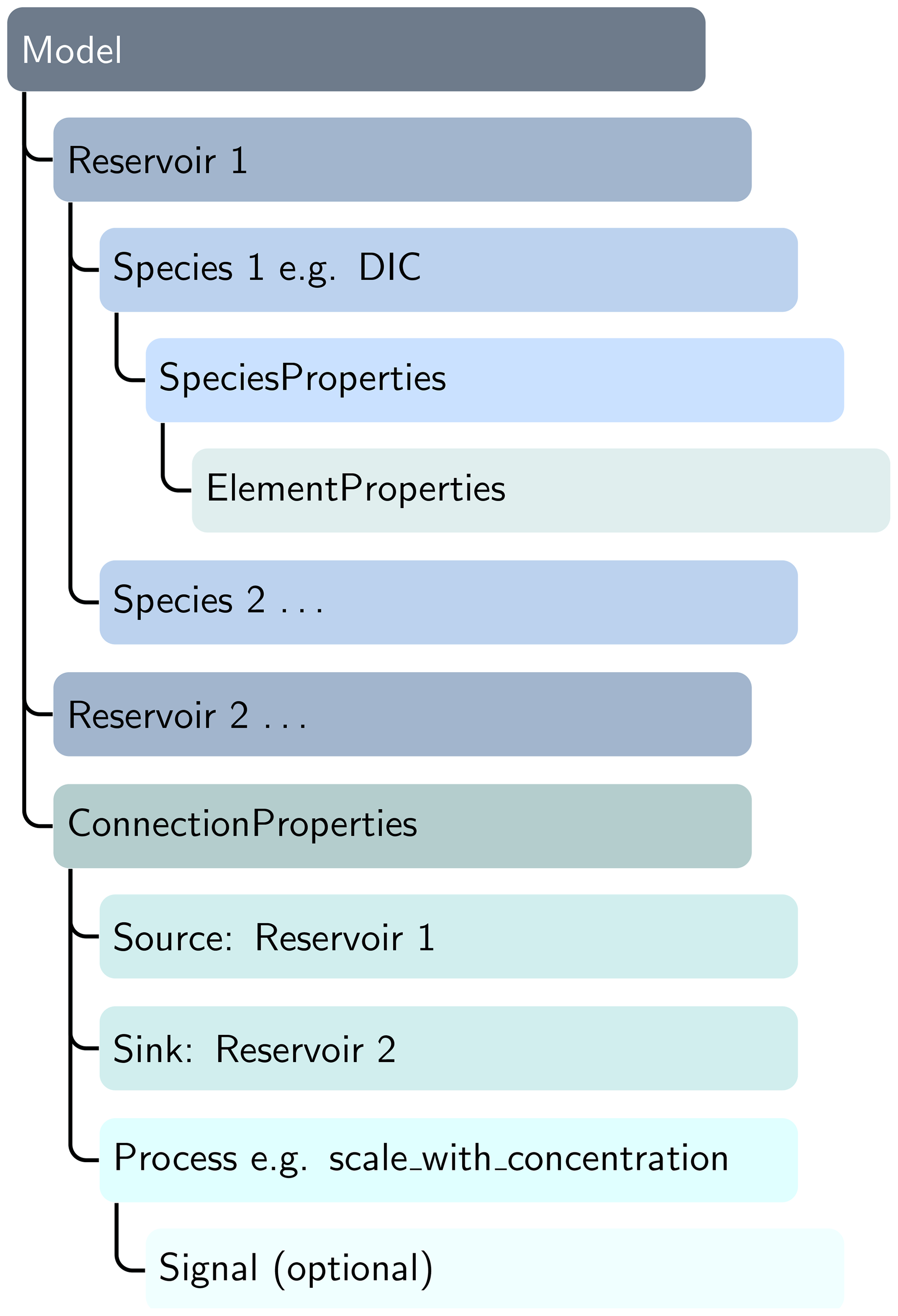
Figure 1 ESBMTK uses a modular hierarchical object structure. ConnectionProperties instances are used to establish a source–sink relationship as well as defining the type of transport process (e.g., scaling a flux by concentration; see, e.g., Listing 1). Connection processes can be modulated by external forcings (signal instances) to evaluate the model response to a perturbation. The object-driven model definition reduces code complexity since a change to the number or type of species automatically propagates to the respective connection instances without the need to adapt the code for these changes. The object instances are stateful, which simplifies introspection and debugging. DIC: dissolved inorganic carbon.

ESBMTK comes with a wide array of predefined processes to connect boxes (e.g., scale a flux relative to another flux, kinetic and equilibrium isotope effects, sediment dissolution, gas exchange). Additionally ESBMTK provides a variety of methods for post-processing and data management (including graphical output) and leverages standard Python methods for introspection and interactive documentation (see the user guide for details, Wortmann, 2025a). While there is no graphical interface similar to Simulink, this approach significantly reduces coding complexity and model development time. Crucially, the model structure is independent of the numerical implementation. Instead, the model is parsed dynamically to create the necessary equation system which is then passed to an ODE solver library like ODEPACK (Hindmarsh, 1992). Separating the model description from numerical implementation results in well-documented model code and combines the computational efficiency of state-of-the-art numerical libraries with the ease of use of Python. Presently, the resulting ODE is coded as Python, but it is possible to modify the parser to output the ODE system in other languages (e.g., Julia).

2 Methods

The following sections are not meant as a user guide; rather, they describe implementation details and the underlying assumptions. The user guide and code examples are available online (see the “Code availability” section below).

2.1 Isotope ratios

Several ESBMTK classes have the option to perform stable-isotope-related calculations, with the important caveat that presently there is no structure for isotope systems with more than two isotopes, nor are there provisions to consider radiogenic isotopes. Further, isotope effects during air–sea gas exchange are currently only defined for CO₂ and O₂. The online user manual describes, however, how to supply the relevant parameters for other gases. In the following, we will only describe the most pertinent implementation details.

To specify the initial isotope ratio of a given species instance, ESBMTK uses the common delta notation; e.g., for ³⁴S and ³²S (sulfur) we can write

$$\begin{array}{}\text{(2)}& \mathit{\delta }{}^{\mathrm{34}}\mathrm{S}=\left({\displaystyle \frac{{\left(\frac{{}^{\mathrm{34}}\mathrm{S}}{{}^{\mathrm{32}}\mathrm{S}}\right)}_{\mathrm{Sample}}}{{\left(\frac{{}^{\mathrm{34}}\mathrm{S}}{{}^{\mathrm{32}}\mathrm{S}}\right)}_{\mathrm{Standard}}}}-\mathrm{1}\right)\times \mathrm{1000}\left[\mathrm{mUr}\mathrm{VCDT}\right].\end{array}$$

The unit is in per mil (i.e., per thousand) or milliurey, where 1 ‰ = 1 mUr (Brand and Coplen, 2012). Although it is customary to combine the unit with the name of the reference standard (e.g., [mUr VCDT]), ESBMTK currently does not parse isotope units; rather, delta must be provided in units of milliurey.

If a connection between two Reservoir instances involves a process that changes the isotope ratio, one can specify the enrichment factor ϵ in the ConnectionProperties, where ϵ is defined as

$$\begin{array}{}\text{(3)}& \mathit{ϵ}=(\mathit{\alpha }-\mathrm{1})\cdot \mathrm{1000}\left[\mathrm{mUr}\right],\end{array}$$

where α equals the isotope fractionation factor between two substances like HCO${}_{\mathrm{3}}^{-}$ and organic matter (OM) during photosynthesis:

$$\begin{array}{}\text{(4)}& {\mathit{\alpha }}_{{\mathrm{HCO}}_{\mathrm{3}}^{-}-\mathrm{OM}}={\displaystyle \frac{{\left(\frac{{}^{\mathrm{13}}\mathrm{C}}{{}^{\mathrm{12}}\mathrm{C}}\right)}_{{\mathrm{HCO}}_{\mathrm{3}}^{-}}}{{\left(\frac{{}^{\mathrm{13}}\mathrm{C}}{{}^{\mathrm{12}}\mathrm{C}}\right)}_{\mathrm{OM}}}}.\end{array}$$

Note that the definition of ϵ is independent of the isotope reference standard, and thus the unit is only given as milliurey. As with delta values, the enrichment factor has to be supplied as a number without units. Internally, ESBMTK only tracks the total concentration and the concentration of the dominant isotope species. The respective delta values are computed once integration has finished. Adding, e.g., isotope fractionation to a given connection (transport process) requires that the respective Reservoir instances have been initialized with a defined isotope ratio and that the connection instance specifies the fractionation factor (see Listing 2).

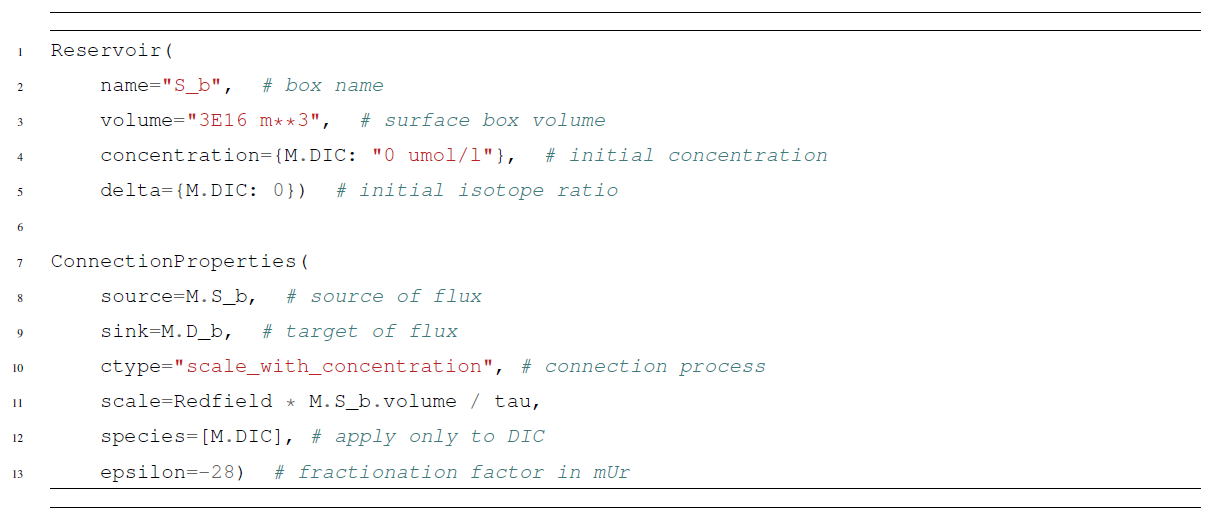
Listing 2 Code fragment showing how to add isotope calculations to a given model (lines 5 and 13). Note that this code will not run by itself. Working examples are provided in the online documentation.

2.2 Weathering

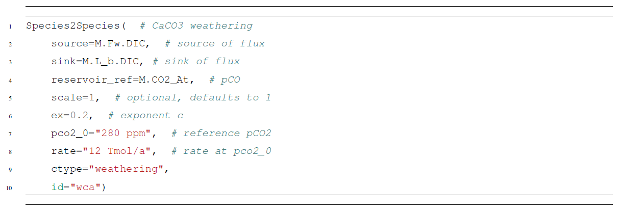
ESBMTK provides a connection type that calculates weathering intensity as a function of CO₂. The implementation is rather simple and follows Walker et al. (1981):

$$\begin{array}{}\text{(5)}& f=A\times f_{\mathrm{0}}\times {\left({\displaystyle \frac{p{\mathrm{CO}}_{\mathrm{2}}}{p_{\mathrm{0}}{\mathrm{CO}}_{\mathrm{2}}}}\right)}^{\mathrm{c}},\end{array}$$

where A denotes the area and f₀ denotes the weathering flux at a given reference pressure p₀CO₂. The CO₂ partial pressure at a given time t is denoted as pCO₂, and c is a constant that defines the strength of the weathering (see Walker et al., 1981, and Listing 3). It is however easy to add a new weathering class to ESBMTK that adds a more comprehensive parameterization of weathering processes.

Listing 3 Code fragment showing how to add a connection between a source (F_w) and sink, where the flux is a function of the CO₂ partial pressure (see Eq. 5).

2.3 Seawater properties and equilibrium constants

Provided that the model is specified in units of mol kg⁻¹ (i.e., substance content; McNaught and Wilkinson, 2019) and that pressure, temperature, and the concentrations of total alkalinity (TA) and total dissolved inorganic carbon (DIC) are known, ESBMTK can calculate a variety of tracers and dissociation constants. The carbonate system dissociation constants are calculated with the PyCO2SYS library, which provides a choice of 4 different pH scales, 18 different parameterizations for the dissociation constants, and various methods to calculate buffer factors (see Humphreys et al., 2022). This approach not only avoids code duplication but also simplifies the comparison between different models. At present ESBMTK supports PyCO2SYS options to select the pH scale and the parameterizations for the dissociation constants.

The solubility of CO₂ is based on the K₀ value returned by PyCO2SYS, which follows Weiss (1974). ESBMTK reports the CO₂ solubility as SA_co2 in mol L⁻¹ atm⁻¹, corrected for water vapor pressure at sea level as a function of temperature and salinity (see Weiss and Price, 1980). Oxygen solubility is based on the parameters listed in Sarmiento and Gruber (2006), and seawater density is calculated using the equation of state given by Zeebe and Wolf-Gladrow (2001).

It should be noted that, presently, the code assumes that neither temperature nor pressure changes during the model run. Therefore thermodynamic and kinetic constants are not updated during the model run. In many cases, this is of no concern since, e.g., during glacial–interglacial changes, the changes to the carbonate equilibrium constants are almost fully compensated by the change in ocean volume and the resulting variations in alkalinity (Zeebe and Wolf-Gladrow, 2001). However, this is not universally true and remains an important trade-off between computational efficiency and precision. Future releases will alleviate this shortcoming.

2.4 Carbon chemistry and carbonate dynamics

ESBMTK uses total dissolved inorganic carbon (DIC) and total alkalinity (TA) as master variables to calculate [H⁺] and seawater carbonate speciation. While TA and DIC fully determine the state of the marine carbonate system, solving for [H⁺] is computationally expensive. Follows et al. (2006) demonstrate that if one knows a suitably close estimate for [H⁺] at t=i, one can estimate [H⁺] at $t=i+\mathrm{1}$ with sufficient precision from the concentrations of [DIC] and [TA] without computational overhead. Provided that the changes in [H⁺] between integration time steps are smaller than $\mathrm{3}\times {\mathrm{10}}^{-\mathrm{11}}$ mol kg⁻¹, the associated error is too small to be of concern (Follows et al., 2006). We therefore use the PyCO2SYS library during the model initialization to compute the initial [H⁺] concentration and then use the iterative algorithm of Follows et al. (2006) in subsequent time steps. ESBMTK will print a warning if the change in [H⁺] exceeds the above threshold. However, during integration, ESBMTK only carries tracers for boron, [H⁺], and [CO₂]_aq. All other carbon species are calculated once the integration finishes.

Carbonate dissolution in the water column and sediments is a function of the saturation state which changes with depth. To calculate the resulting burial and dissolution fluxes, one needs a statistical representation of the relationship of sediment area versus depth. ESBMTK approximates this with a hypsometric curve that is based on a 5 min grid that has been downsampled from the Global Bathymetry and Topography at 15 arcsec (SRTM15+ V2.5.5 dataset; Tozer et al., 2019). The flux calculations use the parameterizations proposed by Boudreau et al. (2010a, b). Their approach first calculates specific depth boundaries (i.e., the saturation depth for CaCO₃ z_sat or the CaCO₃ compensation depth z_cc) as a function of the average CaCO₃ solubility product in the surface ocean ($K_{\mathrm{sp}}^{\mathrm{0}}=\mathrm{4.29}\times {\mathrm{10}}^{-\mathrm{7}}$ mol² kg⁻²), a characteristic depth value ($z_{\mathrm{Sat}}^{\mathrm{0}}=\mathrm{5078}$ m b.s.l.), and the calcium and carbonate ion concentrations (see Fig. 2 for equations). In the second step, they provide a parameterization of the resulting CaCO₃ burial–dissolution fluxes as a function of the carbonate export flux from the surface ocean and the area between the critical depth intervals (e.g., between z_sat and z_cc). It should be noted that Boudreau et al. (2010a) do not consider the aragonite dissolution and that their parameterization assumes an idealized mean ocean temperature distribution and homogeneous carbonate ion concentration in the deep-ocean box (Boudreau et al., 2010b). However, the scheme is computationally efficient and captures transient changes, i.e., times when the snow line and carbonate compensation depth are at different depth levels.

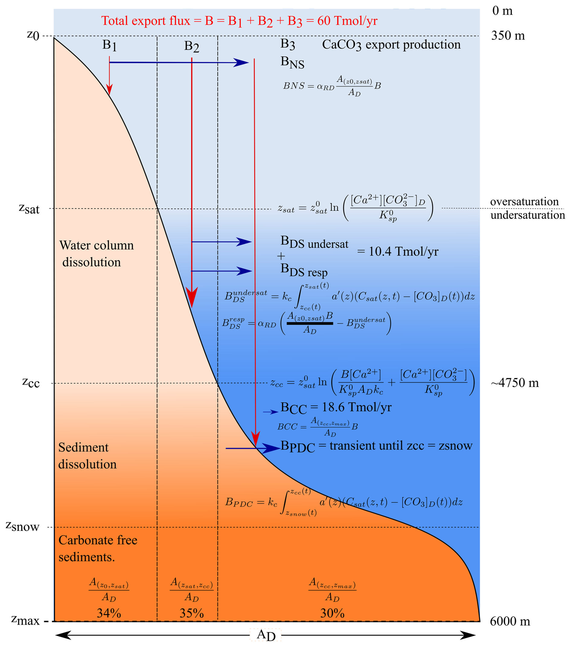
Figure 2 Parametrizations for carbonate burial–dissolution fluxes as proposed by Boudreau et al. (2010a). A denotes cumulative seafloor areas, and B denotes fluxes. The critical depth intervals (z₀, z_cc, z_snow) denote the separation between the saturated and undersaturated waters and between carbonate-bearing and carbonate-free sediments. B_NS denotes sedimentary calcite dissolution from oxic respiration, B_DS denotes the dissolution by respiration in the sediments and in dissolution in the water column, B_CC denotes the dissolution below the carbonate dissolution depth, and B_PDC denotes the transient dissolution if the depth of z_cc and the snow line diverge from each other. α is the fraction of CaCO₃ that dissolves above the saturation horizon z_sat.

2.5 Gas reservoirs and air–sea gas exchange fluxes

ESBMTK provides a GasReservoir class that can be used to track concentration changes in, e.g., pCO₂. In its default setting, this class uses a mass of 1.78×10²⁰ mol for the earth's atmosphere and tracks a given species as the mole ratio relative to the atmosphere. While this class can be used to track several species (e.g., O₂ and pCO₂), they are currently treated as independent of each other. Further, changes in a given species's concentration will not affect the overall mass of the atmosphere. The error associated with typical variations in pCO₂ is however negligible.

Gas exchange between two Reservoir instances is implemented as a connection instance that requires a GasReservoir and a regular Reservoir instance that carries seawater tracers (see above). The gas exchange implementation follows Zeebe (2012):

$$\begin{array}{}\text{(6)}& F_{\mathrm{gas}}=A\cdot u\left(\mathit{\beta }\cdot p{\mathrm{CO}}_{\mathrm{2}}-{\left[{\mathrm{CO}}_{\mathrm{2}}\right]}_{\mathrm{aq}}\right),\end{array}$$

where [CO₂]_aq denotes the concentration of CO₂ in solution (in mmol kg⁻¹) and pCO₂ denotes the atmospheric CO₂ concentration (in ppm). A denotes the surface area, u denotes the piston velocity, and β denotes the solubility of CO₂. Currently, ESBMTK provides these parameters for CO₂ and O₂.

Listing 4 Example showing how to explicitly specify the equilibrium and kinetic isotope fractionation factors during gas exchange. Note that presently these are not updated during the model run.

Isotope fractionation effects related to the exchange of CO₂ across the air–sea interface assume that the isotope ratios of HCO${}_{\mathrm{3}}^{-}$ and DIC are roughly equal. This simplification introduces a small error of up to 0.3 mUr at 20 °C and a pH between 7.5 to 8.2 (see Zeebe, 2012), and we calculate the gas exchange flux for ¹³C as

$$\begin{array}{}\text{(7)}& F_{\mathrm{gas}{}^{\mathrm{13}}\mathrm{C}}=A\cdot u\cdot {\mathit{\alpha }}_{\mathrm{u}}\left(\mathit{\beta }\cdot {\mathit{\alpha }}_{\mathrm{dg}}\cdot p{}^{\mathrm{13}}{\mathrm{CO}}_{\mathrm{2}}-{\mathit{\alpha }}_{\mathrm{db}}\cdot R_{\mathrm{T}}\cdot {\left[{\mathrm{CO}}_{\mathrm{2}}\right]}_{\mathrm{aq}}\right),\end{array}$$

where α_u denotes the kinetic fractionation factor during gas exchange (equivalent to an ϵ value of 0.8 mUr; Zhang et al., 1995), α_dg denotes the equilibrium fractionation factor between CO₂ in solution and CO₂ in gas (ϵ=1.076 mUr; Zeebe and Wolf-Gladrow, 2001), and α_db denotes the equilibrium fractionation between dissolved CO₂ and HCO${}_{\mathrm{3}}^{-}$ (ϵ=9.36 mUr; Zeebe and Wolf-Gladrow, 2001). ESBMTK provides the respective fractionation factors for CO₂ and O₂. For other gases, these factors can be specified in the ConnectionProperties (see Listing 4).

2.6 Model perturbations

A key element in box modeling studies is to force one or more model boundary conditions, e.g., CO₂ emissions. ESBMTK provides the signal class that implements methods to create square, pyramidal, and bell-shaped signals, as well as a method to read forcing data from a CSV (comma-separated values) file. The signal data can be interpreted either as an absolute flux that is added to an existing flux or as a multiplier that is used to increase/decrease a given flux. Furthermore, signal instances can be added together to create arbitrarily complex shapes. Signal data are automatically truncated and/or padded to match the model time domain, and the data are resampled so that they match the model time step. However, care must be taken that signal duration is at least 4 times as long as the model time step. Signal instances are then associated with one or more connection instances. See the code example in Listing 5.

Listing 5 Example on how to create a signal and associate it with a given connection instance to create a transient pulse in the riverine PO₄ flux. The online manual provides further examples.

2.7 Numerical implementation

ESBMTK defaults to an implicit backward differentiating ODE solver that is suitable for the typically stiff problems in earth sciences. Specifically, we use the scipy.integrate.BDF solver as provided by the SciPy library which builds on the algorithms by Byrne and Hindmarsh (1975), Hairer et al. (1993), and Shampine and Reichelt (1997). This algorithm uses a variable time step and automatically increases the time step until the solution becomes unstable. ESBMTK defaults to an initial time step of 1 s. While this seems short given geological timescales, setting this value to a longer time interval has no perceptible influence on the execution time since the solver rapidly increases the integration interval. Conversely, however, setting this value too high can affect the stability of the carbonate system solution. This is particularly true for small-scale models that, e.g., model the acidification of distilled water in a beaker.

A challenge with variable-time-step algorithms is that they cannot account for the nature of episodic events, such as volcanic eruptions or anthropogenic carbon inputs driving the model. The ESBMTK model class thus provides the max_timestep keyword that limits the solver to time step values that are smaller than this value. While the BDF (backward differentiation formula) solver is not sensitive to scaling problems (i.e., differences between variables that are very small and those that are very large), its convergence criterion needs to be adjusted for variables that differ by orders of magnitudes. ESBMTK does this based on the initial values of the respective species so that the absolute tolerance value t is

$$\begin{array}{}\text{(8)}& t={\mathrm{10}}^{-\mathrm{7}}\times v,\end{array}$$

where v denotes a given variable value. In other words, for a concentration value of 28 mM, the solution must be within $\pm \mathrm{2.8}\times {\mathrm{10}}^{-\mathrm{6}}$ mM.

3 Proof of concept

In order to show the versatility of ESBMTK and to test the model results, we implement the Boudreau et al. (2010a) model using the ESBMTK library. The model code and associated scripts are available online (see the “Code availability” section below). The Boudreau et al. (2010a) model consists of three ocean boxes, one for the low-latitude ocean areas, one for the high-latitude ocean areas, and one for the deep ocean. Additionally, it has a box representing the atmosphere (see Fig. 3).

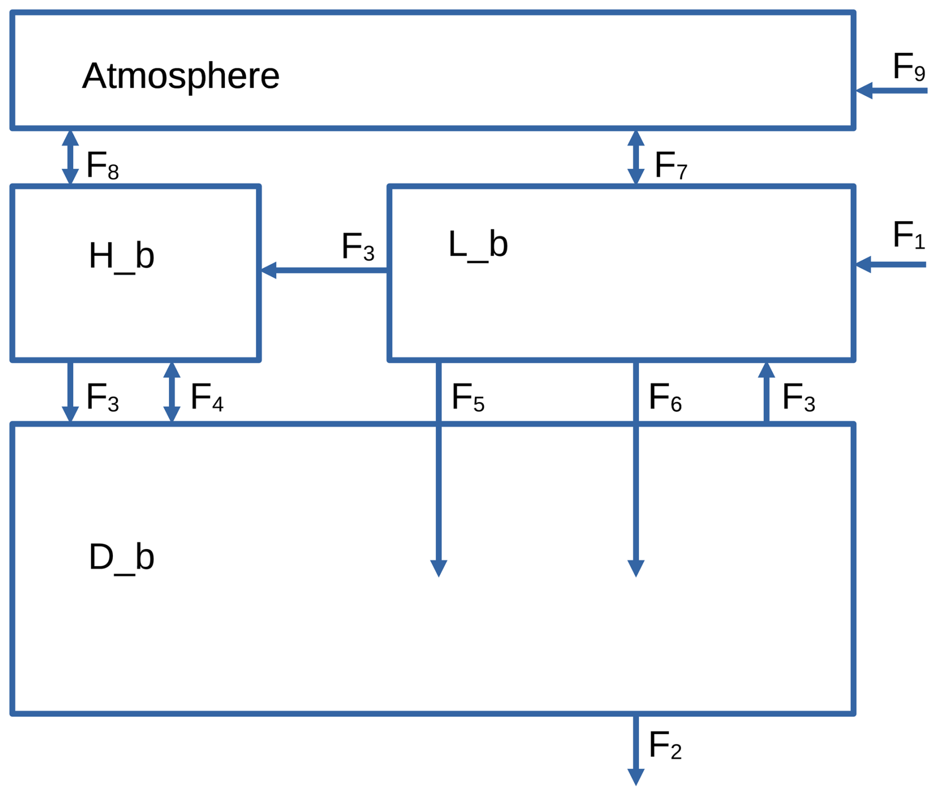
Figure 3 Model geometry used by Boudreau et al. (2010b). See text for flux descriptions and Table 2 for flux values. Note that fluxes can denote more than one species; e.g., F₆ stands for the carbonate export flux that will affect dissolved inorganic carbon (DIC) as well as total alkalinity (TA).

The model assumes that there is no organic and inorganic export flux from the high-latitude to the deep-ocean box and that the particulate organic matter flux from the low-latitude to the deep-ocean box (F₃) is fully remineralized and has no effect on alkalinity. The carbonate export flux (F₆) is partly dissolved and partly buried (F₂), while the partitioning between F₂ and F₆ depends on the carbon speciation in the deep box. The model uses a fixed rain ratio, where ${\mathrm{F}}_{\mathrm{5}}/{\mathrm{F}}_{\mathrm{6}}=\mathrm{0.3}$. Alkalinity and dissolved organic carbon are replenished via a constant weathering flux (F₁). The model does not consider phosphor cycling. Thermohaline circulation (F₃) and mixing between the high-latitude and deep-ocean boxes (F₄) redistribute the dissolved species, and gas exchange with the atmosphere balances the concentration of dissolved CO₂ between the low-latitude and high-latitude boxes (F₇ and F₈). Model parameters are given in Tables 1–4.

Table 1 Geometry and P–T conditions for the Reservoir boxes in the Boudreau et al. (2010a) model. All boxes use a salinity of 35.

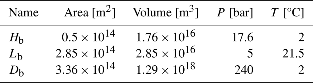
Table 2 Flux parameters as used by Boudreau et al. (2010a). The DIC and alkalinity burial flux F₂ is a function of the export productivity and CO${}_{\mathrm{3}}^{\mathrm{2}-}$ concentration in the deep box (see Fig. 2). The gas exchange fluxes F₇ and F₈ are a function of the dissolved CO₂ concentrations in the surface boxes.

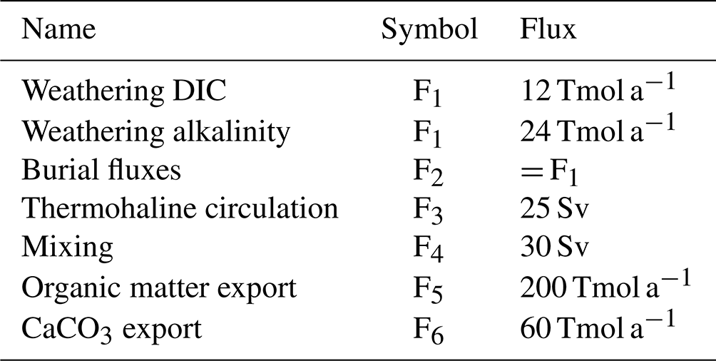
Table 3 Biogeochemical rate parameters as used in the ESBMTK version of the Boudreau et al. (2010a) model. With the exception of α, all parameters after Boudreau et al. (2010a).

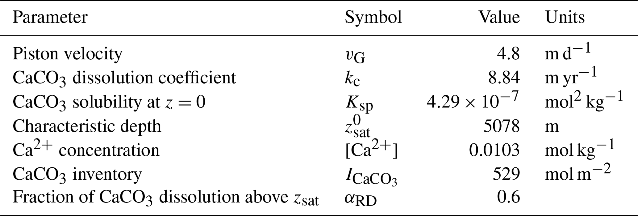
Table 4 Equilibrium constants as used in our implementation of the Boudreau et al. (2010a) model (where K0 denotes the solubility coefficient for CO₂ in seawater, K1 and K2 are the first and second dissociation constants of carbonic acid, KW is the ion product of water, and KB is the dissociation constant of boric acid). These values are computed by PyCO2SYS (Humphreys et al., 2022) based on the P–T values in Table 1 and reported relative to the free pH scale. The concentration values for DIC and TA are the steady-state concentrations in the ESBMTK version of Boudreau et al. (2010a). The steady-state values of the original model are in brackets. The steady-state pCO₂ in the ESBMTK model is 270 ppm; Boudreau et al. (2010a) do not list their steady-state pCO₂.

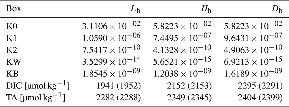
Figure 4 Comparison between the model results reported by Boudreau et al. (2010a) and the ESBMTK-based implementation. Solid lines denote the ESBMTK results, and dotted lines denote data that have been digitized from the figures in Boudreau et al. (2010a). See text for discussion. gex in panel (d) stands for gas exchange.

Boudreau et al. (2010b) use the equilibrium constants parameterization of Millero et al. (2006) and report their results on the free pH scale. However, they do not report the fractional value used for the dissolution above the saturation horizon (α_RD). Manual tuning of the ESBMTK implementation suggests that a value of 0.6 results in steady-state conditions similar to the values reported by Boudreau et al. (2010b) (see Fig. 4). We then use these steady-state conditions to force the model with a CO₂ pulse (F₉) that is based on the IS92a emission scenario (Leggett et al., 1992) but uses a Gaussian evolution after 2100 that peaks near the year 2250. The total CO₂ emission equals 4025 Gt C over 600 years, and Boudreau et al. (2010a) assume that there is no terrestrial carbon uptake. Figure 4 shows a comparison between the ESBMTK-based model implementation and the data reported by Boudreau et al. (2010a).

Both models demonstrate that the CO₂ release (Fig. 4g) increases the CO₂ fluxes across the air–sea interface (Fig. 4d) and the increase in ocean water acidity due to the dissolution of CO₂. This causes a rapid rise in the saturation horizon (z_sat; Fig. 4e), a fairly rapid rise in the carbonate compensation depth (z_cc; Fig. 4e), and a slower rise in the snow line (z_snow; Fig. 4e). Consequently, the carbonate burial flux decreases and the carbonate dissolution flux increases (Fig. 4h), elevating the DIC and TA concentrations in all ocean boxes. The increase in TA enhances the ocean's buffer capacity, leading to a rapid drawdown of atmospheric CO₂ after the year 2320 (Fig. 4f). However, returning to preindustrial steady-state values requires the re-equilibration of the marine alkalinity pool, a process that occurs over hundreds of thousands of years. For a detailed interpretation of the model results, refer to the original publication by Boudreau et al. (2010a).

4 Discussion

The steady-state results of the ESBMTK model not only broadly match the data of Boudreau et al. (2010a) but also show noticeable differences. This is particularly true for the low-latitude ocean, where both the DIC and TA steady-state concentrations are lower than those in the original model (11 and 6 µmol, respectively; see Table 4), which in turn affects the gas exchange fluxes (Fig. 4d). In the deep box, the DIC concentration is 4 µmol higher and the TA concentration is 5 µmol higher than in the original model, resulting in a slightly higher CO${}_{\mathrm{3}}^{\mathrm{2}-}$ concentration (87.4 versus 86 µmol kg⁻¹ in the original model), deepening the location of the critical horizons by about 63 m.

The differences between the low-latitude surface box and the deep ocean are mainly controlled by the export productivity and the burial–dissolution fluxes as well as the thermohaline upwelling. Productivity and upwelling velocity are known constants, and the burial–dissolution fluxes equations are known as well. However, the fraction of carbonate dissolution (α_RD) above the saturation horizon is not mentioned by Boudreau et al. (2010a). Increasing α until the surface DIC and TA values better match the original model, however, increases the respective differences in the deep box. This in turn increases the CO${}_{\mathrm{3}}^{\mathrm{2}-}$ concentrations and deepens the depth of the z_sat, z_cc, and z_snow horizons by another 50 m and further reduces the steady-state pCO₂. Carbon speciation in the deep box would also be affected by the choice of dissociation constants, but it is also conceivable that the differences are caused by the underlying hypsographic data.

We cannot exclude the possibility that there is a numerical error in the ESBMTK library, but it is more likely that the observed variations are caused by small differences in the dissociation constants and/or hypsometric data. Both ESBMTK and Boudreau et al. (2010a) use the carbon dissociation constants parameterization of Millero et al. (2006); however, both rely on third-party libraries (PyCO2SYS and AquaEnv, respectively) to calculate the k values, and we were unable to compare the constants used in our model with the constants used in the original model.

Boudreau et al. (2010a) provide a non-steady-state case to test the response of the system against the release of 4025 Gt over 600 years. We digitized the forcing function for our model from Fig. 2 in Boudreau et al. (2010a). Integration of the digitized data yields a total carbon mass of 4590 Gt C instead of 4025 Gt. We, therefore, scale the digitized data by a factor of 0.877, which results in the differences shown in Fig. 4g. Using the solid line in Fig. 4g as a forcing function, our model yields results that are similar to the original model. While the CaCO₃ burial and dissolution fluxes are similar, the long-term response in the deep-ocean alkalinity is among the more visible differences. However, overall, the ESBMTK implementation replicates the result of the original model well.

5 Conclusions

ESBMTK started as a teaching tool, with the idea of emphasizing model geometry and processes over coding details. This is particularly true for conceptually simple models in combination with Jupyter Notebooks, an approach that has been successfully used in classes of undergraduates that had no previous coding experience. Advanced students with basic Python skills benefit from using ESBMTK by being able to focus on the inherent complexities of model definition, rather than being sidetracked by numerical issues. This approach significantly reduces model development time and ensures that the object-based modeling results in well-documented code that is easy to read with a basic understanding of Python syntax. The hierarchical, object-oriented program structure provides a robust framework for experienced Python programmers to adapt or extend the ESBMTK library. These features are also attractive in a research environment, significantly improving readability and reproducibility without incurring major performance penalties.

Rather than implementing our parameterizations for the various equilibrium constants, we use the well-tested PyCO2SYS library, which provides access to a wide range of published equilibrium constants and a choice of different pH scales. At present, carbonate chemistry computations are based on previously published algorithms that are suitable for the modern ocean but will require adaptions for conditions where the deep ocean is warmer than today. Likewise, at present the model is only valid for modern ocean Ca and Mg concentrations and considers calcium carbonate but not aragonite. We also note that the current 0.14.x version of the library does not update kinetic and thermodynamic constants during model execution. Re-implementing a previously published model that uses the same carbon chemistry algorithms, we find that the results of both models are in good agreement. We do observe, however, small differences that we attribute to minor variations in the underlying carbon species equilibrium constants.