An enhanced emission module for the PALM model system 23.10 with application for PM₁₀ emission from urban domestic heating

This article presents an enhanced emission module for the PALM model system, which collects discrete emission sources from different emission sectors and assigns them dynamically to the prognostic equations for specific pollutant species as volumetric source terms. Bidirectional lookups between each source location and cell index are maintained by using a hash key approach, while allowing all emission source modules to be conceived, developed, and operated in a homogeneous and mutually independent manner. An additional generic emission mode has also been implemented to allow for the use of external emission data in simulation runs. Results from benchmark runs indicate a high level of performance and scalability. Subsequently, a module for modeling parametrized emissions from domestic heating is implemented under this framework, using the approach of building energy usage and temperature deficit as a generalized form of heating degree days. A model run has been executed under idealized conditions by solely considering dispersion of PM₁₀ from domestic heating sources. The results demonstrate a strong overall dependence on the strength and clustering of individual sources, diurnal variation in domestic heat usage, and the temperature deficit between the ambient temperature and the user-defined target temperature. Vertical transport additionally contributes to a rapid attenuation of daytime PM₁₀. Although urban topology plays a minor role on the pollutant concentrations at ground level, it has a relevant contribution to the vertical pollutant distribution.

1 Introduction

Air pollution is one of the largest environmental and health risk factors in the European Union (EU; EEA, 2023). Despite ongoing efforts at improving general air quality, concentrations of airborne pollutants, such as particulate matter (PM₁₀), still frequently exceed EU standards across the 27 EU nations. It is particularly severe in urbanized areas, where 97 % of the population was exposed to PM at concentrations above guideline levels set forth by the World Health Organization in 2021 (EEA, 2023). Accordingly, a high population density also results in a larger variety of anthropogenic emission sources in urban agglomerations. In addition to sectors in road traffic as well as industry and energy production, heat generation through stationary combustion in residential and commercial buildings – collectively termed domestic heating – can be a significant source of pollutants (Baumbach et al., 2010), constituting about 10 % of urban emissions for nitrogen oxides (NO_x) and PM₁₀ (Senatsverwaltung Berlin, 2019; Pültz et al., 2023). To this end, urban-scale models such as the PALM model system (Maronga et al., 2020) are indispensable tools for the evaluation of urban air quality. They can be deployed to assess the impact of different emission reduction strategies or urban planning exercises for improving air quality (Jeanjean et al., 2017; Piroozmand et al., 2020; Chan and Butler, 2021).

As emission data are often required as input to these models at high temporal and spatial resolutions (Guevara et al., 2020; Chan et al., 2023), a suitable methodology for generating and handling such emission data is critical for obtaining reliable pollutant dispersion and transformation characteristics through numerical model runs at such a scale. In the implementation of the PALM model system (Maronga et al., 2020), emissions can only be modeled as boundary conditions on surface-bound grid cells. Based in part on the existing surface module (Gehrke et al., 2021), time-varying emissions of a given pollutant species, e.g., particulate matter (PM₁₀) from vehicle traffic and domestic heating, are to be aggregated across all source locations. They are then introduced into the solution domain as time-varying surface fluxes. This approach was used to provide hourly traffic emissions, in which three different levels of detail (LODs) are available (Khan et al., 2021). Typically, emission sources are fully parametrized under LOD 0, through, for instance, redistribution of aggregate values according to rudimentary input information for characterizing surrogate activity data (Gruney et al., 2017). On the other hand, the user has the option of supplying already processed input emission data under LOD 2, independent of any predetermined parametrization schemes. Partial parametrization, or LOD 1, is another available option where emissions are estimated from aggregated levels through corresponding user-defined surrogate activity data.

Emission sources are typically categorized into sectors, exemplified by definitions in the Nomenclature for Reporting (NFR). For conceptual generalization, different production mechanisms under each sector can be classified as such. However, additional flexibility should be provided to account for different emission source types (e.g., point, line, and area sources) as well as the physical mechanisms of pollutant formation within each sector. For example, PM₁₀ emissions from road traffic can originate from combustion products or from abrasion and resuspension sources, each requiring different physical parametric treatments (Chan et al., 2023). Moreover, biogenic emissions such as isoprene (Guenther et al., 1991, 1993, 1999) and pollen (Zink et al., 2012, 2013) contain different physical mechanisms and model treatments for emission release and replenishment. Thus, the architecture and application of the emission sources in this framework should be organized in a similar fashion as found in prominent chemical transport models such as WRF-Chem (Grell et al., 2005) and LOTOS-EUROS (Manders et al., 2017). On the other hand, as they ultimately contribute to the source and sink terms of the prognostic equation for the corresponding species, the numerical construct of all emission sectors share certain common elements, in which abstractions can be drawn across all relevant sectors to afford systemic uniformity and code reusability, significantly simplifying design, development, and deployment.

In addition, while a majority of emission sectors – such as traffic and domestic heating – are released as fluxes near the surface, i.e., ground or roof, this is not always the case. In particular, depending on the grid resolution, large emission sources – such as pollutant source terms from the European Pollutant Release and Transfer Register (E-PRTR) and point-source information from the Gridding Emission Tool for ArcGIS (GRETA; Schneider et al., 2016) – could be introduced over a vertically distributed region above the respective industrial stack. Furthermore, emissions from elevated sources – such as biogenic emissions from trees and exhaust emissions from aviation – cannot always be represented as surface fluxes at urban scales, where grid resolution can be sufficiently high that they no longer take place on the first vertical layer alone. Conversely, at sufficiently low horizontal resolutions, it becomes more likely that a given cell location could contain contributions from multiple emission sectors. Although this could be partially addressed using the current surface-flux-based approach, in which emissions are to be assembled a priori as surface flux boundary conditions, a yet greater degree of flexibility and independence can be achieved if they could be introduced directly as volumetric source terms, where emission contributions could be specified independently of each other at different points in time and at different LODs.

The objective of this article is to introduce an enhanced emission module for the PALM model system, available from version 23.10 onwards. This module offers a high level of flexibility, implementation modularity, ease of use, and computational performance. As an illustrative example, this new methodology is applied to parametrize emissions from domestic heating sources, based on the energy demand approach of Baumbach et al. (2010) and Struschka and Li (2019). The numerical performance of the enhanced emission module is evaluated using a synthetic test case executed at different levels of domain decomposition. This is concluded by a demonstration in a residential region in Berlin under idealized conditions.

2 Model description

2.1 Theoretical foundations

Consider the incompressible prognostic equation at the resolved scale for the concentration of a given pollutant species p, denoted as ξ_p, including net source term contributions:

$$\begin{array}{}\text{(1)}& {\partial }_t{\mathit{\xi }}_p+u_i{\partial }_i{\mathit{\xi }}_p-{\mathrm{\Gamma }}_p{\partial }_j^{\mathrm{2}}{\mathit{\xi }}_p=\sum _r{\mathit{\sigma }}_p^{\mathrm{r}}+\sum _m{\mathit{ϵ}}_p^m,\end{array}$$

where Γ_p is the diffusivity of species p, ${\mathit{\sigma }}_p^{\mathrm{r}}$ is the corresponding net chemical conversion rate of species p from all relevant reactions r, and ${\mathit{ϵ}}_p^m$ is the net emission rate of p originating from all relevant emission sectors m. The treatment of the ${\mathit{\sigma }}_p^{\mathrm{r}}$ terms has been thoroughly discussed in Khan et al. (2021); the present work thus concerns the incorporation of the ϵ_p terms into Eq. (1).

While the chemical production terms σ are continuous in space and time and are calculated everywhere in the computational domain by solving a set of ordinary differential equations for temporal integration specific to a predetermined chemical kinetic mechanism (Damian et al., 2002), the ϵ terms are only defined at sparse, discrete regions and are not always continuously active depending on the emission sector. This represents, for instance, emissions from domestic heating through chimneys or road traffic. Since emissions are typically supplied into the model as a mass or molar input rate (i.e., mol s⁻¹ or kg s⁻¹), provided through either inventories (Jähn et al., 2020; Murphy et al., 2021) or parametrization (Huszár et al., 2010; Mues et al., 2014; Ge et al., 2020), converting these rates into concentration rates ϵ can be done by dividing the input rate with the corresponding mass or molar density at the computational cell where emissions take place. Therefore, ϵ can be effectively regarded as a volume source. In terms of computer processing and storage, it is strongly preferred to only consider ϵ_p at discrete locations where the emission source is present. However, there are three challenges associated with this approach, and the emission module architecture must be conceived so as to accommodate them in a sufficiently simple yet computationally robust and efficient manner:

1. As emission sources are discrete, contiguity in the associated data structures (such as arrays) in the emission module no longer reflects the spatial continuity in the computational domain.

2. The heterogeneity of emission sources from different sectors must be implicitly considered to enable different independent methods for parametrization and production mechanism specification.

3. The interface between the prognostic equation solver and the emission module should be implemented to only allow localized data access to prevent propagation of data corruption into other emission sectors.

Traditionally, discrete emission sources can be represented within a contiguous multidimensional array covering the horizontal domain up to a predetermined vertical level, as implemented in some regional-scale models (e.g., Grell et al., 2005). However, this approach requires a large amount of available memory and storage, increasing with the number of grid cells, as most cell locations in this array do not contain emission sources. For urban scales such as in PALM, where grid resolutions can be as high as 1 m, this resource penalty can severely impede scalability and runtime performance.

To overcome this restriction, all emission sources within an emission sector can be amalgamated into a one-dimensional data structure known as a hash map (Cormen et al., 2009), h^m, where the spatial association between the individual emission source location and the corresponding (i, j, k) grid index locations in the computational domain are maintained by assigning a hash key, κ, unique to each location. In the meantime, a global hash map, H, accumulates all emission source data across all relevant emission sectors for each location and assigns them as source terms (${\mathit{ϵ}}_p^m$) to the corresponding prognostic equations indicated by their hash keys κ. In this approach, the volume sources are stored in a simple and compact array, with one entry for each volume source. Memory is thus only allocated in proportion to the number of volume sources, substantially reducing runtime resource consumption.

For a uniform Cartesian grid, as used in PALM, the hash map for each emission sector, h^m, containing the mapping between the (i, j, k) grid location of each emission source and the corresponding hash key κ can be represented in a one-dimensional array:

$$\begin{array}{}\text{(2)}& \begin{array}{rl}{h}^{\mathrm{m}}=\mathit{\left\{}{\mathit{\kappa }}^m\right(i,j,k):& {\mathit{\kappa }}^m\in W^{N_{\mathit{\kappa }}^m},\\ & i\in W^{N_i^m},j\in W^{N_j^m},k\in W^{N_k^m}\mathit{\}},\end{array}\end{array}$$

where W denotes a set of natural numbers, i.e., $W\in \mathrm{0},\mathrm{1},\mathrm{2},\mathrm{\dots }$ up to (but not including) the corresponding upper bound N.

In a 3D Cartesian system, the hash key κ can be derived from a linear mapping of the cell indices:

$$\begin{array}{}\text{(3)}& \mathit{\kappa }=N_i\left(k{N}_j+j\right)+i,\end{array}$$

where N_i and N_j are the cell counts along the two horizontal axes in the computational domain. Other methods for determining κ exist, such as using different cell index ordering in Eq. (3) or by using bitwise operations (Jenkins, 1997; Teschner et al., 2003), which are more suitable for unstructured grid model systems such as Chan and Butler (2021). As PALM is a Cartesian grid model system, a unique, bidirectional mapping between the grid cell indices and corresponding hash keys can be achieved with Eq. (3) alone.

Thus, the volumetric emission source term can be expressed as the product between the source function $f_p^m$ for emission sector m at each emission source location defined in h^m:

$$\begin{array}{}\text{(4)}& {\mathit{ϵ}}_p^m=h^{\mathrm{m}}\cdot f_p^m\left(t,{\mathit{\kappa }}^m|{\mathit{\eta }}_p^m\right),\end{array}$$

where f^m is a function of time (t), position (expressed succinctly in terms of κ), and additional sector-specific parameters (η^m) for pollutant species p that are defined, for instance, when parametrization is involved. In turn, the transference of the sectoral emission sources to the linear system of discretized prognostic equations for species p (${\sum }_m{\mathit{ϵ}}_p^m$) is the union of all emission sectors, in which values belonging to the same hash key for species p are summed across all hash maps containing it:

$$\begin{array}{}\text{(5)}& \sum _m{\mathit{ϵ}}_p^m=\bigcup _m{\mathit{ϵ}}_p^m,\end{array}$$

where ⋃ is the union operator. In practice, the hash map belonging to each emission sector m is amalgamated into a global hash map H, where

$$\begin{array}{}\text{(6)}& H=\bigcup _m{h}^{\mathrm{m}},\end{array}$$

and the source terms for each pollutant species p under each sector m is added directly to the corresponding species prognostic equations as required at each source location by looking up its (i, j, k) cell indices from its hash key κ. This eliminates the need for intermediate data storage for source term accumulation.

2.2 Overall architecture

Figure 1 illustrates the overall architecture of the enhanced emission module. Owing to different emission production mechanisms, emission source data (${\mathit{ϵ}}_p^m$) for pertinent pollutant species (p) originating from each emission sector (m) are encapsulated in dedicated Fortran modules. Access for emission source data is restricted to standardized interface subroutines to prevent direct or accidental interference from other modules. Each module under this framework also maintains a separate hash map (h^m) to indicate corresponding source locations represented by the hash key (κ). Beyond the physical mechanisms, all modules are similarly constructed so that new emission sectors can be introduced easily.

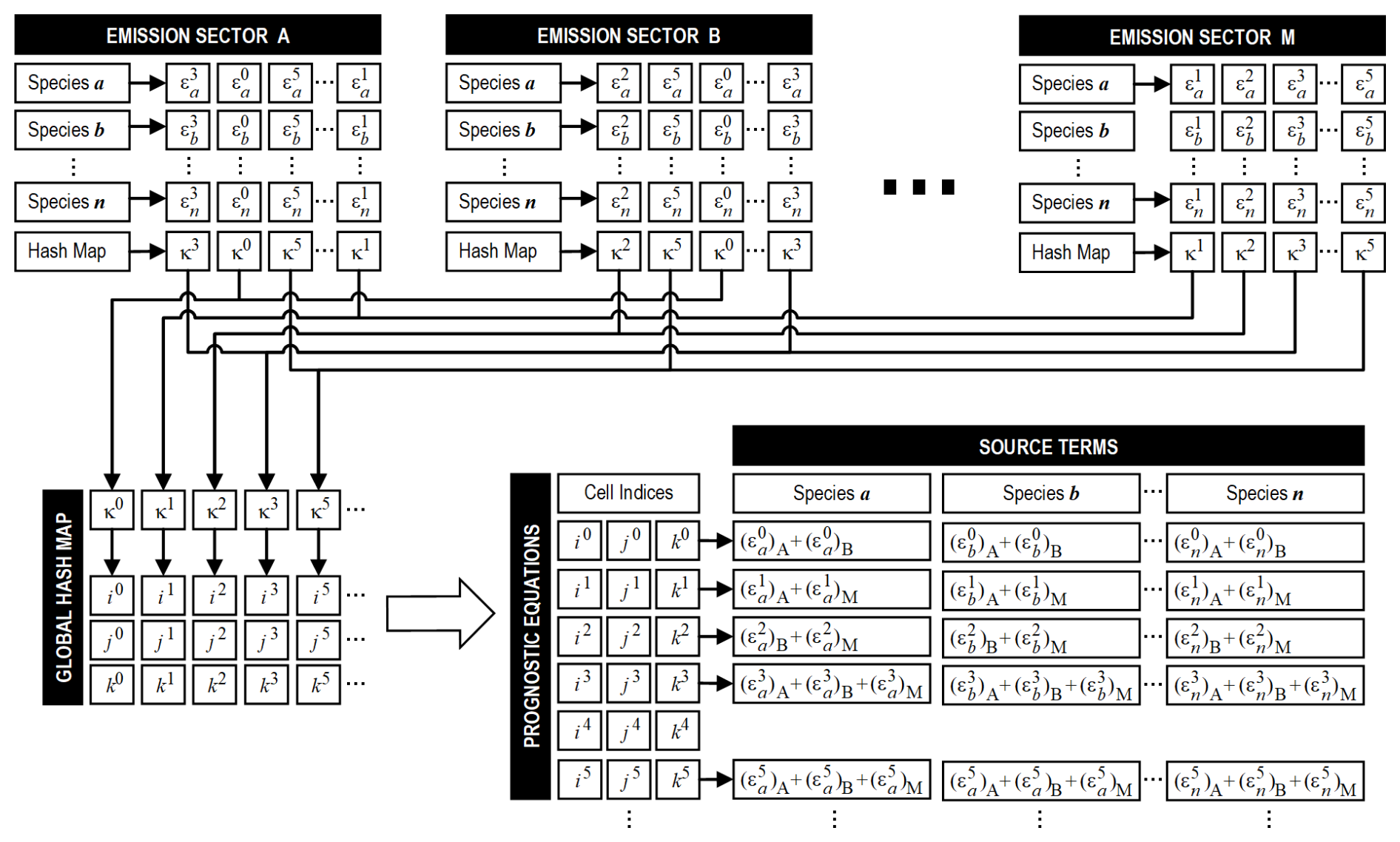
Figure 1 Overall architecture of the enhanced emission module in the PALM model system. Chemical species are indicated by lowercase letters (a, b, c, etc.), and emission sectors are in uppercase letters (A, B, C, etc.); n and M denote an arbitrary number of species and emission sectors, respectively. Hash keys (κ) and corresponding cell indices (i, j, k) are distinguished by superscript numerals.

The hash map for all emission sectors (h^m) will be merged to form a separate global hash map (H), which contains the (i, j, k) indices of all cells containing an emission volume source, as well as their respective hash keys (κ). The global hash map (H) and all associated subroutines and functions are contained in a separate module, whose interface is accessible by both the emission module and the prognostic equation solver. In this way, sector-specific emission sources (${\mathit{ϵ}}_p^m$) can be accumulated into the prognostic equation source terms at the correct cell locations. The global hash map also serves as a barrier between the prognostic equation solver and the emission module under this architecture. As such, new emission sectors can be developed without introducing code changes outside the chemistry module in the PALM model system.

2.3 Implementation in the PALM model system

The enhanced emission module has been implemented and released for the PALM model system 23.10 (Maronga et al., 2020). This includes the parametrized domestic heating module described in Sect. 3. Both models are part of the chemistry module, and the interested reader is encouraged to refer to Khan et al. (2021) for further details.

2.3.1 Program flow

Design decisions made on the overall architecture are based on user specifications on each LOD and active pollutant species. The LOD defines the extent of parametrization that takes place for an emission sector. Meanwhile, the emitting species relevant to the emission sector of interest can also be defined as input. Thus, provisions should be given to render their treatment flexible. Each emission sector may operate in up to three levels of detail. Typically, LOD 0 indicates full parametrization, where all sector-specific parameters are defined solely in the namelist file. On the other hand, in LOD 2 the user must provide all emission source data covering the duration of the model run. Partial parametrization is referred to as LOD 1, which requires both user emission data and namelist parameters as inputs. These sector- and LOD-specific parameters are analogous to the ${\mathit{\eta }}_p^m$ term in Eq. (4). As input data, only user-specified species that appear in the chemical mechanism will participate in the model run. Any species not defined by the user (or defined by the user but not appearing in the chemical mechanism) will be ignored. Species specifications are to be performed independently for each emission sector.

Figure 2 shows the hierarchy of the new emission module within the PALM model system. The existing emission module is currently under the chemistry module (chemistry_model_mod). The new modules reside within the dotted line region, which includes chem_emis_vsrc_mod, modules dedicated to each emission sector (chem_emis_[sector]_mod), and a module for the generic mode emission (chem_emis_generic_mod). Their roles in the enhanced emission module will be detailed in the paragraphs below. Other modules that directly interact with the chemistry module are collectively referred to as the core, and optional input data for each emission sector, i.e., netCDF files required for user-defined emission data specification (otherwise known as level 2 of detail or LOD 2), are not shown in Fig. 2. Each computational domain maintains its own hash maps (h^m and H), as each domain is geographically distinctive, allowing emission sources to be assigned locally to the corresponding prognostic equations.

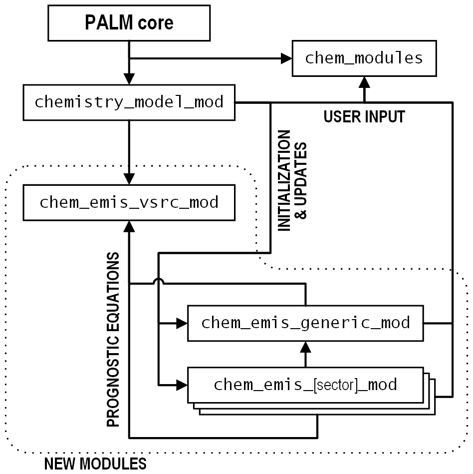
Figure 2 Hierarchy of the new source files (inside the dotted line region) introduced for the enhanced emission module of the the PALM model system. Arrows indicate the direction of module access.

The module chem_modules contains definitions of all parameters that can be specified by the user in the namelist file (_p3d), and it has been modified to contain activation and configuration options for individual emission sectors. Subroutine entry points for each emission sector are also introduced in the module chemistry_model_mod for initialization, as well as emission source updates at specified intervals during the model run. The new module chem_emis_vsrc_mod contains the global hash map (H), where accumulation of prognostic equation source terms takes place through linkage to the hash maps of all activated emission sectors (h^m). The interface between chemistry_model_mod and the core modules in the PALM model system remains unchanged.

2.3.2 Emission module code structure

A structural overview of the Fortran modules for each emission sector (m) is presented in Fig. 3. It comprises an interface to external modules and components; a data storage component for various sector-specific parameters such as LOD, active pollutant species information, and hash key linkage to the prognostic equations; and methods (i.e., subroutines and functions) for general and LOD-specific operations and data manipulation. Data storage for each emission sector is kept private and can only be accessed through the publicly defined interface subroutines. This ensures encapsulation of modular data and functionality. The interface serves as a wrapper for all internal functions and subroutines, which are expected to be uniform for the emission module.

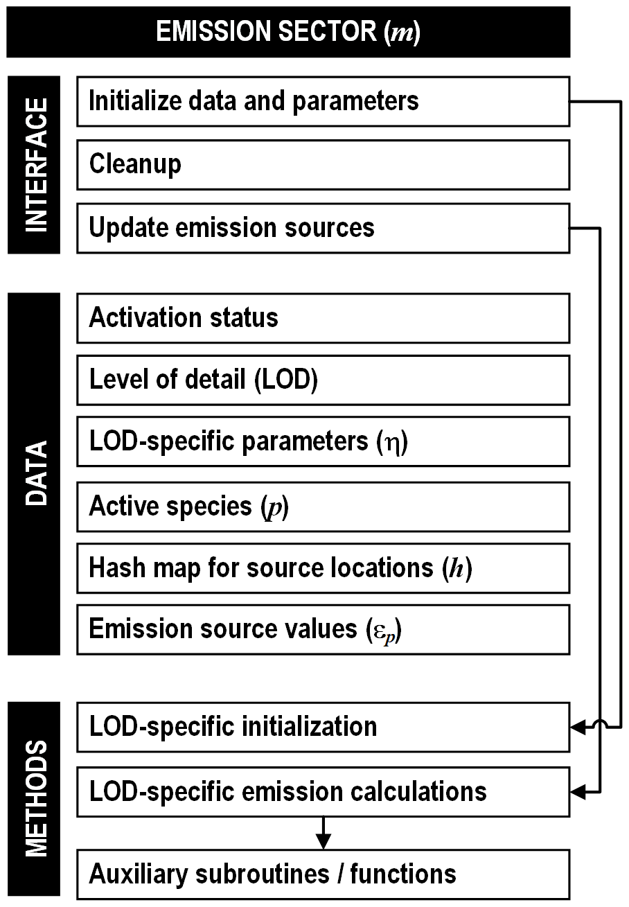
Figure 3 Overall structure of a module for an emission sector under the enhanced emission framework. Module data and methods are encapsulated, to be accessed externally through the use of interface subroutines.

There are three subroutines defining the interface. First is initialization, which assigns user-defined data values specified in the namelist file (_p3d) as well as other optional external data sources. Throughout the model run, emission source values will be updated based on values at specific points of simulation time. This is done in the PALM model system core by calling the update subroutine defined in the interface, which, in turn, invokes internal sector and LOD-specific subroutines for emission source calculation. A corresponding cleanup function is called upon termination of the emission sector module to release all resources allocated during the model run.

The user can specify which sector(s) is to be activated for a model run and, if so, the corresponding LOD. The LOD-specific parameters, represented by the ${\mathit{\eta }}_p^m$ term in Eq. (4), are also internal within each emission sector. The user can also specify the pollutant species (p) to be used in the model run, which will be linked to the chemical species in the active chemical mechanism. Meanwhile, the hash map (h^m) contains information on all cell locations of emission sources through their hash keys (κ). Access between the individual source locations and the corresponding prognostic equation is established through the linkage between h^m and the global hash map located in the module chem_emis_vsrc_mod, where all entries are sorted using an implementation of the qsort algorithm (Bentley and McIlroy, 1993) to facilitate the hash key lookup, such that the runtime scales only with the logarithm of the number of emission sources using bisection search.

As mentioned in Sect. 2.3.1, the manner with which the emission module can be initialized and how its emission sources are to be updated are subject to the LOD. These specific subroutines and functions can be declared and implemented based on development specifications and requirements. In addition, implementation of various physical mechanisms and numerical constructs specific to the emission sector can be further abstracted into auxiliary subroutines and functions, which can be introduced at initial design or at subsequent development iterations as needed.

2.3.3 Generic emission mode

An additional generic mode has been introduced to provide an alternate possibility to provide emission source data for which an explicit emission sector is not (yet) available in the PALM model system. The generic emission mode contains no parametrization. Thus, it is only available under LOD 2, in which the temporal and spatial generic emission sources can be introduced into the model in a separate file in netCDF format. As such, the preparation and generation of these generic mode emission data can be done outside the PALM model system, thus maximizing user flexibility. Furthermore, as LOD 2 data under various emission sectors are implemented in the same manner, the Fortran module for the generic emission mode also contains common functions and subroutines that can be used in other emission sectors. These include but are not limited to user-defined and mechanism pollutant species matching, update interval detection, and basic data structure initialization and manipulation.

3 Parametrized emissions from domestic heating

As an illustrative example, the underlying theory for parametrized (LOD 0) domestic heating, as well as its implementation under the framework described in Sect. 2.1, will be discussed. In addition, the test runs outlined in Sects. 3.3 and 4 will also be based on this emission sector, from which computational performance and model results will be presented and accordingly discussed.

3.1 Emission source parametrization

The theoretical foundations for parametric modeling of domestic heating emissions are derived from the work of Baumbach et al. (2010) and Struschka and Li (2019), which are based on a direct relationship between emissions and energy usage. Emissions are calculated using the so-called emission factors, which vary with the pollutant species and the furnace technology. On the other hand, daily energy consumption is a function of the size, geometry, age, and function of the individual buildings. These form the two aspects of the discussion below. Typically, buildings with a footprint (i.e., projected ground area) of less than 10 m² and a mean height of less than 3 m are not considered in the calculation.

The daily energy usage of a building (E_B) can be expressed as a ratio between its annual aggregate and the number of degrees of temperature below the target temperature. In addition, diurnal variations due to general anthropogenic activity (i.e., heat tends to be turned up during early mornings and evenings and turned down while sleeping) are also considered:

$$\begin{array}{}\text{(7)}& E_B\left(t\right)=\left({\left.{\displaystyle \frac{E_B}{\mathrm{\Delta }T}}\right|}_A\right)\mathit{\zeta }\mathrm{\Delta }T\left(t\right),\end{array}$$

where ${\left.E_B\right|}_A$ is the annual energy consumption for heating of building B; ΔT|_A is the annually accumulated temperature deficit, also known as heating degree; ΔT(t) is the current temperature deficit, a generalized form of heating degree day (HDD) to diurnal variations; and ζ is the diurnal variation in domestic heat usage, such as that defined by the Copernicus Atmosphere Monitoring Service (CAMS) for domestic and commercial combustion, under Gridded NFR (GNFR) sector C for other stationary combustion (Kuenen et al., 2022).

The annual energy consumption for heating (E_B|_A) takes into account the volume, compactness, and energy demand of the building type (β), defined in Table B1:

$$\begin{array}{}\text{(8)}& {\left.E_B\right|}_A={\left.E_{\mathit{\beta }}\right|}_A{\mathrm{\Phi }}_{\mathit{\beta }}{V}_B,\end{array}$$

where Φ_β is the compactness factor of building type β belonging to building B, ${\left.E_{\mathit{\beta }}\right|}_A$ is the annual energy demand of building type β per unit footprint area, and V_B is the volume of building B. Typically, ${\left.E_B\right|}_A$ takes up 80 % of the total energy consumption of the building (Mues et al., 2014). This will be implemented in upcoming versions of the parametrized domestic emission model.

The compactness factor, in units of m⁻¹, is a density indicator for the building. On the other hand, the annual energy demand, in units of J m⁻² per annum, is the footprint-specific energy consumption. Tabulated values of these two quantities can be found in Table B2 for each building type (β).

In turn, the temperature deficit ΔT(t) is calculated by subtracting the target indoor temperature (T₀) from the outdoor ambient temperature (T_∞):

$$\begin{array}{}\text{(9)}& \mathrm{\Delta }T\left(t\right)=max\left\{\mathrm{0},\left[T_{\mathrm{0}}-T_{\mathrm{\infty }}\left(t\right)\right]\right\}.\end{array}$$

When the ambient temperature (T_∞) is greater than the target temperature (T₀), there will be no temperature deficit (i.e., ΔT=0), and it is assumed that no heating will be required.

The volumetric emission for each species p can then be calculated for each source location – represented by the corresponding hash key κ – using Eq. (4). Here, the parameters, i.e., η in Eq. (4), are represented in terms of the emission factor ψ_p and building energy usage E_B, as shown in the relation below:

$$\begin{array}{}\text{(10)}& f_p\left(t,\mathit{\kappa }|{\mathit{\psi }}_p,E_B\right)={\mathit{\psi }}_p{E}_B,\end{array}$$

where ψ_p is the emission factor for the emitting species, whose values are tabulated in Table B3, and E_B is the building energy usage determined in Eq. (7). It should be noted that ψ_p is a constant normalized by the building energy consumption (E_B) which, in turn, is a function of diurnal anthropogenic activities (ζ) and temperature deficit (ΔT(t)).

To reduce computational effort, PM₁₀ is assumed to be an inert species. However, it is possible to integrate the PALM chemistry module (Khan et al., 2021) with other aerosol models, such as SALSA (Kurppa et al., 2019) and ISORROPIA (Nenes et al., 1998; Fountoukis and Nenes, 2007). On the other hand, it is expected that bulk and turbulent flows are the dominant modes of particulate transport. Gravitational effects, i.e., settling and buoyancy, have not been considered in this case. The interested reader can refer to Khan et al. (2021) for the overall treatment of gravitational effects for dry deposition in the PALM chemistry module.

3.2 Module implementation

The domestic emission module is implemented in the PALM model system under chem_emis_domestic_mod. In accordance with the overall architecture in Figs. 2 and 3, interaction between the domestic emission model and PALM are made through the following interface subroutines:

• chem_emis_domestic_init( ),

• chem_emis_domestic_update( ), and

• chem_emis_domestic_cleanup( ),

which handle LOD-specific module initialization, update of emission sources during the solver iterations, and relinquishing of allocated resources, respectively. The implementation of the fully parametrized (LOD 0) emission source term calculations is based on the formulation outlined in Sect. 2.1, and the user-defined emission source terms make use of interface functions and subroutines already defined in the generic emission mode described in Sect. 2.3.3. All options and parameters are defined in module chem_emission_mod, and they can be specified by the user using the namelist file (_p3d).

The activation of the domestic emission parametrization can be specified by setting the namelist option emis_domestic to .TRUE., while the corresponding LOD is specified using the option emis_domestic_lod. Currently, full parametrization (LOD 0) and user-specification (LOD 2) are available. Under LOD 2, the time series of all emission volume sources (that is, their cell locations and the emission level) will be provided by the user explicitly through the input file with the suffix _emis_domestic in netCDF format, and no further namelist options are required. On the other hand, with LOD 0, additional parameters, presented in Table 1, can be specified by the user.

Table 1 Namelist options for domestic emission parametrization (LOD 0).

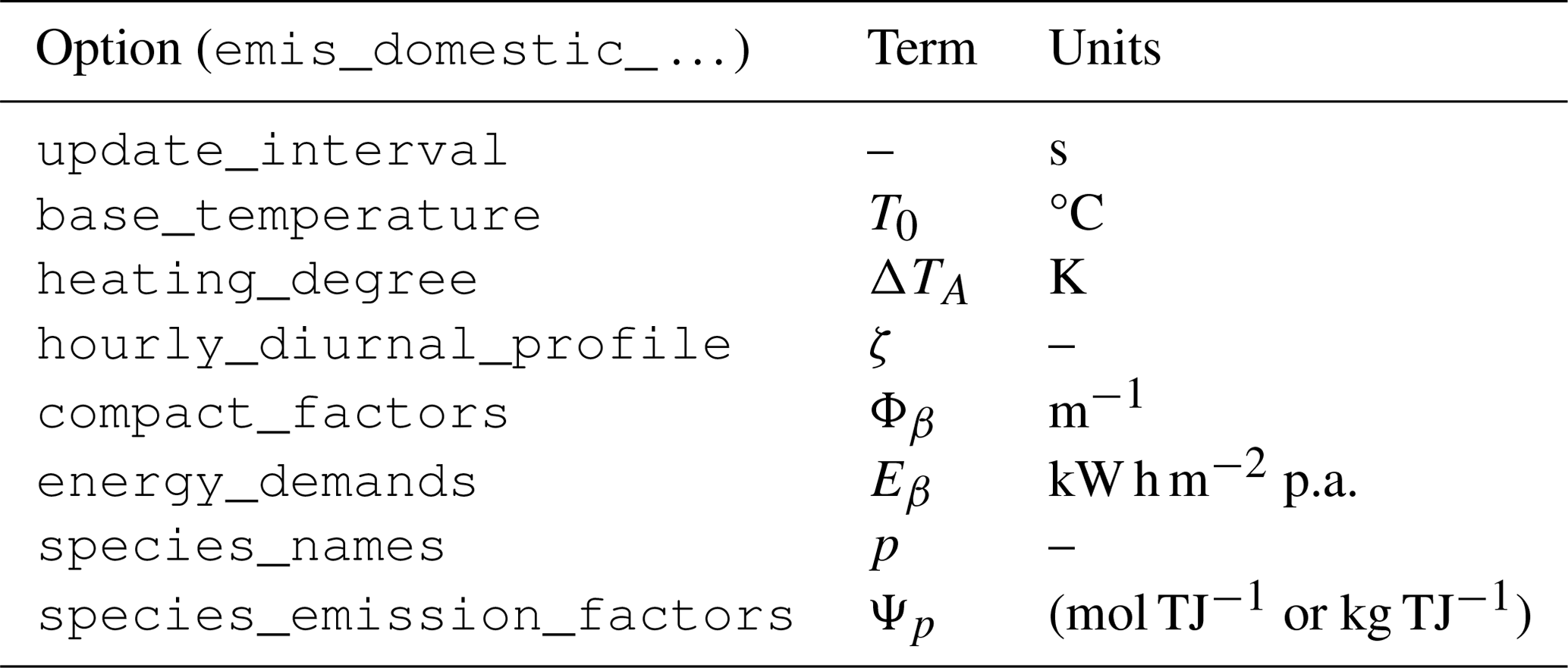
The emission sources at each building stack location are updated at the start of the model run and again afterward at every interval specified by the option emis_domestic_update_interval, which is 300 s by default. A user-defined target temperature, with a default set to 15 °C (VDI, 2013), can be defined through the option emis_domestic_base_temperature, where domestic heating is assumed to be turned on when the ambient temperature falls below this target temperature. On the other hand, the option emis_domestic_heating_degree specifies the annual cumulative temperature (in degrees of temperature) to be heated above the ambient temperature to the target temperature, with a default value of 2100 K. The diurnal heat usage profile can be defined on an hourly basis via the option hourly_diurnal_profile, where the user can specify an hourly weighting to represent aggregate anthropogenic activity for the region of interest. As default, the CAMS diurnal profile for residential and commercial combustion, defined under the GNFR sector C (other stationary combustion), is used (Kuenen et al., 2022). The compact factors and energy demands for each building type (see Appendix B) can be provided with the options emis_domestic_compact_factors and emis_domestic_energy_demands. The default values for both are defined in Table B2.

Meanwhile, emission factors are to be presented in a name–value pair, where the species names are defined with the option emis_domestic_species_names. The corresponding emission factors are provided on the basis of unit energy consumed with the option emis_domestic_species_emission_factors. The emission factors for airborne species are to be presented in units of mol TJ⁻¹ and those for particulate species (such as PM₁₀) and other inert species are to be presented in kg TJ⁻¹. As the definition of chemical species in the PALM model system is mechanism-specific, the user must supply the appropriate species names and emission factors and is thus encouraged to refer to Table B3 for representative values of emission factors with different furnace technologies.

Furthermore, for LOD 0, two additional variables defined in the _static file are to be read as input. The first is stack_building_volume, which indicates the (i, j) cell location of each building stack and its corresponding building volume (V_B), typically assigned to each building belonging to a unique building ID. The second is building_type, which contains the type of building (β) defined in Table B1, from which the compactness factor (Φ_β) and energy demand (E_β), e.g., in Table B2, can be found. While the onus is on the user to ensure correctness of all parameter input values, all user inputs will be inspected, in which case invalid entries will be replaced with the default values listed in Appendix B. In addition, a lower limit of zero is imposed on all emission values to ensure a seamless model run.

3.3 Performance benchmark

To provide an estimate of computational performance of the enhanced emission module, a synthetic test case with a horizontal grid size of 400 × 400 cells has been created for evaluation. The test case domain contains 15 vertical layers with 129 600 uniformly distributed sources, representing 5.4 % of the total cell count. Runs were conducted at three different levels of horizontal domain decomposition: 10 × 10 processors (40 × 40 cells per compute core), 20 × 20 processors (20 × 20 cells per core), and 40 × 40 processors (10 × 10 cells per core). A simulation period of 3600 s is set for all cases at a fixed time step of 200 ms so that performance comparison across all runs can be made at a per time step basis. Mass conservation in the solution domain is verified by comparing the total input emission rate of an inert pollutant species (e.g., PM₁₀) into the solution domain to its total mass contained within a cyclic lateral boundary arrangement. All runs were performed on the supercomputer system hosted by the North German Association of High Performance Computing (Norddeutscher Verbund für Hoch- und Höchstleistungsrechnen; HLRN) using compute nodes comprising two Intel® Xeon® Platinum 9242 processors, totaling 96 cores, operating at a base frequency of 2.3 GHz, and 384 GB of physical memory. The PALM model system has been compiled under mpiifort version 2018.6.288 with OpenMPI version 3.1.5.

At each domain decomposition level, control model runs are first conducted with the emission module deactivated, followed by corresponding runs using the emission module. Thus, the runtime for the processing and solving of emission sources, which takes place every time step, can be calculated by taking the difference in the prognostic equation solver times between the domestic and reference runs. A set of 20 control and emission model runs are conducted for each domain decomposition level, and the runs with the two fastest and slowest prognostic equation solver times are discarded to attenuate outlier influence. Summary statistics are performed at both the aggregate level (i.e., all emission sources) and for a single emission source. Ultimately, the per time step runtimes for processing an emission source and prognostic equation are calculated, with corresponding serial performance data extrapolated from the three parallel runs, to evaluate the computational effort of the enhanced emission module.

Table 2 shows the runtime required to complete one time step of the prognostic equations for the control and emission model runs at the three domain decomposition levels, along with results of statistical tests, based on results of $\mathrm{20}-\mathrm{4}=\mathrm{16}$ samples for each model run. To establish statistical significance for the differences in runtimes between the domestic and control runs at each level of domain decomposition, inference in variance uniformity is first established by way of f tests to determine whether the pooled (statistically similar variance) or unpooled (statistically different variance) t tests should be used. A level of significance of 0.05 is used as guideline for all statistical tests.

Table 2 The per time step mean [ms] and variance [ms²] for the prognostic solver runtime for control runs and emission module runs at each domain decomposition level, along with effective DOF [ ] from Eq. (11), statistical significance [ ] for variance uniformity (f test), and sample difference (t test). The number of samples is 16 for all runs, and the level of significance is set to 0.05.

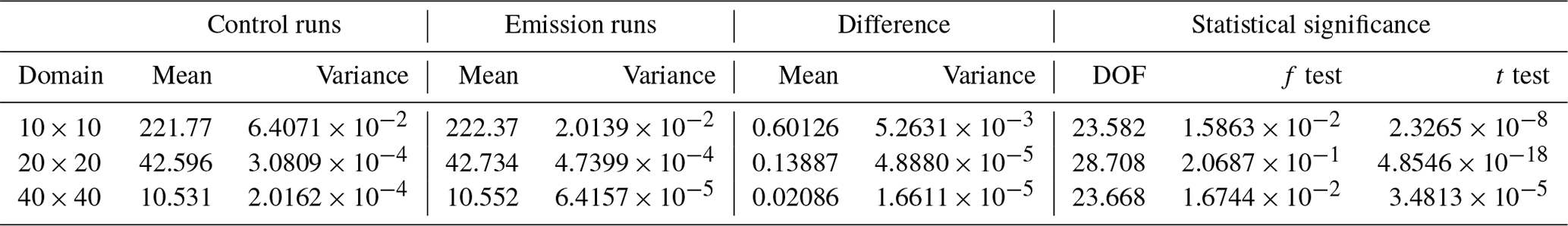
The f tests are performed using $\mathrm{16}-\mathrm{1}=\mathrm{15}$ degrees of freedom (DOF). From the results of the f test, the differences in runtimes are shown to be statistically significant for decomposition levels 10 × 10 (0.0159) and 40 × 40 (0.0167). On the other hand, the difference at level 20 × 20 (0.207) is statistically inconclusive. The decision is thus made to use the unpooled treatment for domestic and control runtime distributions for the subsequent t test, in which the effective DOF is calculated using the Welch–Satterthwaite equation:

$$\begin{array}{}\text{(11)}& {\text{DOF}}_{\text{effective}}={\displaystyle \frac{{\left[{\left(s^{\mathrm{2}}/n\right)}_{\text{domestic}}+{\left(s^{\mathrm{2}}/n\right)}_{\text{control}}\right]}^{\mathrm{2}}}{[\frac{{\left(s^{\mathrm{2}}/n\right)}^{\mathrm{2}}}{n-\mathrm{1}}{]}_{\text{domestic}}+[\frac{{\left(s^{\mathrm{2}}/n\right)}^{\mathrm{2}}}{n-\mathrm{1}}{]}_{\text{control}}}},\end{array}$$

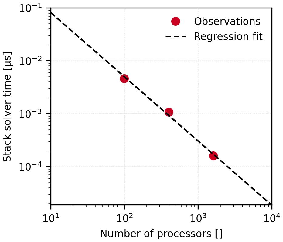
where s² is the unbiased variance estimator of each sample group (i.e., emission and control runs), and n represents the corresponding sample size (16 in both cases). The results from the t test show that the difference in distributions for the runtimes of the domestic and control runs are, indeed, statistically significant at all domain decomposition levels. This also means the corresponding difference can be interpreted as the runtime for the emission module. The differences in runtime for each decomposition setting were normalized by the total number of emission sources (129 600) to assess the numerical performance of the domestic emission module and the volume source emission processing on a per stack or volume source basis for each time step. The time required to complete a time step of the prognostic equations for each volume source is presented in Fig. 4 and Table 3, which can be linearized into a double logarithmic scale, from which the serial performance can be estimated by way of linear regression. This is determined to be 1.3249 µs, representing the upper limit under the current computing software and hardware configurations, with a coefficient of determination of 0.9946. This corresponds to a 0.512 % of serial processing time for all volume sources in the computational domain, where a slight improvement under parallelization can be seen up to 0.198 % with 40 × 40 processors. Therefore, the benchmark demonstrates the effectiveness and scalability of the present emission module, as well as other emission sectors utilizing the volume-source-based emission processing framework.

Figure 4 The per time step stack solver runtime at different domain decomposition levels.

4 Exemplary model run with parametrized emissions from domestic heating under idealized conditions

An idealized run case is conducted, following the performance benchmark, to assess the parametrized domestic emission module as an isolated emission source. The domain of this case study is located in an 800 × 800 m² cardinally aligned region at the border between the Gesundbrunnen and Prenzlauer Berg districts of Berlin, at a horizontal resolution of 2 m, as shown in Fig. 5. The reference coordinate of the region is set to 52°32^′32.6^′′ N, 13°23^′46.5^′′ E and is affixed to the origin of the computational domain. An arbitrary reference elevation of 36.87 m above sea level is also introduced, determined internally by the PALM model to optimize the number of grid points above ground level, from which the vertical (z) dimension of the computational domain extends to another 800 m above. A uniform grid spacing of 2 m was used in the z direction, rendering the domain size of 400 × 400 × 400 cells. The namelist settings for the chemistry parameters for the present run can be found in Appendix C.

Table 3 Stack processing time and total solver runtime per time step for each emission volume source.

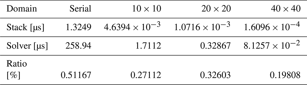
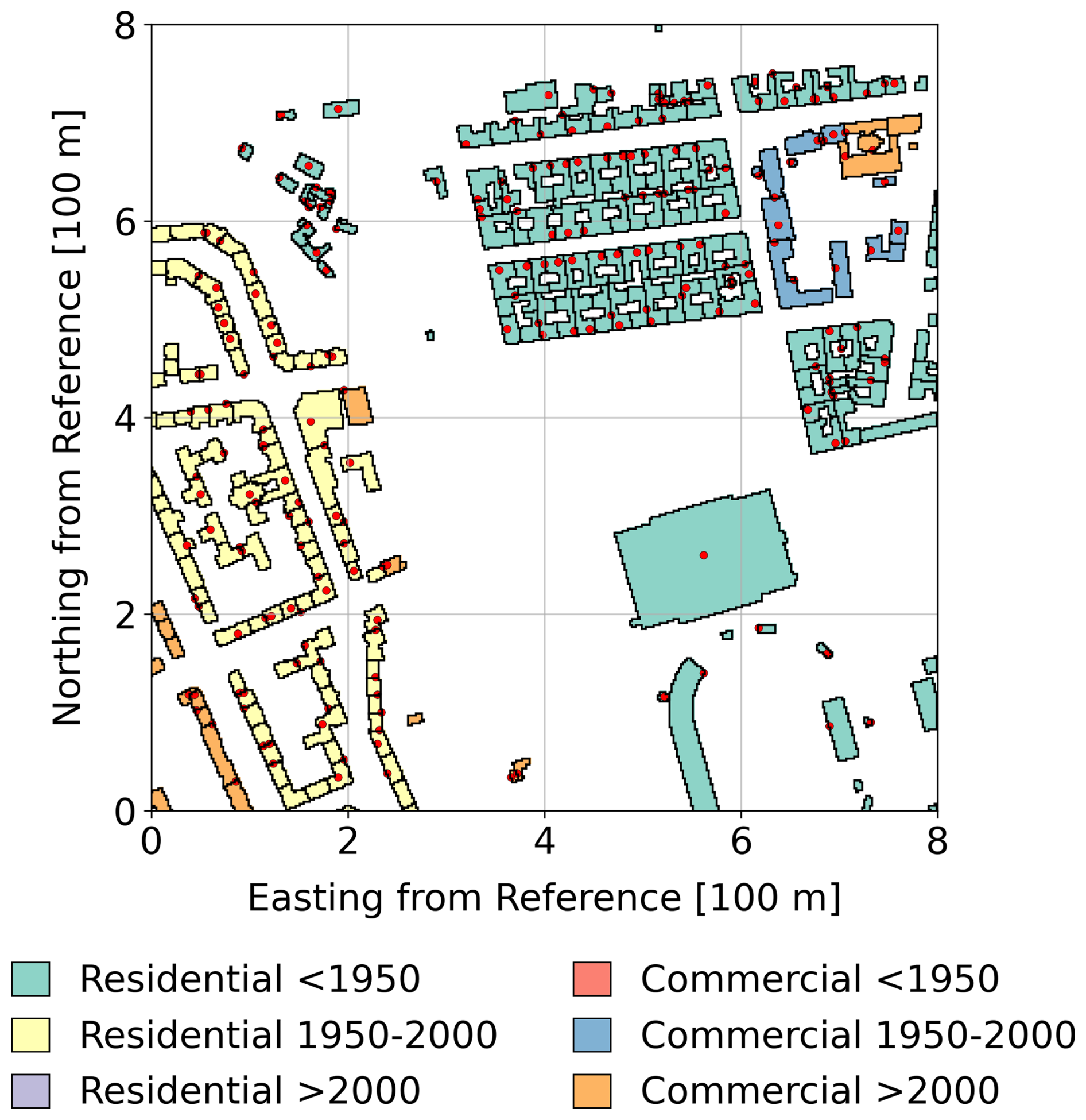
Figure 5 Horizontal distribution of urban structures residing in the region of interest for the idealized model run. Color indicates the building type (Table B1). The locations of chimney stacks are shown by circular red markers. The domain origin is set to 52°32^′32.6^′′ N, 13°23^′46.5^′′ E.

In the parametrization of domestic heating emissions, 228 out of 283 building units have met the minimum height (3 m) and footprint (10 m²) criteria for which stacks are assigned. Emissions of inert PM₁₀ are parametrized for this idealized run. Reactive gas-phase pollutants such as NO and NO₂ are not considered, as their computed concentrations also depend on contributions of other reactive species from the background and other emission sectors not considered in this model configuration. It is also assumed that the pollutants emitted from the stacks are immediately well mixed with the surrounding air in the colocated grid cell. As such, the effects of micromixing resulting from segregation are not expected to be significant at such fine grid resolutions (Mastorakos, 2003; Gamory et al., 2009). The amount of pollutant species emitted from each domestic stack at any given time is calculated in accordance with the parametrization schemes set forth in Baumbach et al. (2010) and Struschka and Li (2019), described in Sect. 3.1. All buildings in the computational domain are assumed to be heated using a mixture of 50 % centralized gas and 50 % oil furnaces (Table B3), according to the building technology data collected by the city of Berlin for the region (Senatsverwaltung Berlin, 2010). The CAMS diurnal profile for residential and commercial combustion under GNFR sector C (Kuenen et al., 2022) is used for the calculation of the weighted temperature deficit profile (ζΔT(t)).

To further simplify the model, static profiles for meteorology have been used for initialization. A horizontal wind of (u, v) = (1.5, 0.5) m s⁻¹ is prescribed to provide constant bulk air movement. An initial temperature of 275 K with a vertical gradient of −0.1 K per 100 m is also introduced on the lateral boundaries to maintain a positive temperature deficit, ΔT(t), throughout the run. A Dirichlet–Neumann boundary condition pair is applied for chemical species (i.e., PM₁₀) at each set of opposing lateral boundaries, while the Neumann boundary condition is applied to the top and bottom of the boundaries of the solution domain. Furthermore, the following modules are also used to provide additional parametrization for relevant physical processes in the PALM model system under large-eddy simulation (LES) mode:

1. the land surface model (Gehrke et al., 2021) to solve for the energy balance of various surface types,

2. the plant canopy model (Maronga et al., 2020) for the parametrization of dynamic and thermodynamic processes of trees and vegetation,

3. the parametrized surface radiation scheme for calculating the radiative energy budget under clear-sky conditions (Maronga et al., 2020), and

4. the online chemistry module to model the dispersion of PM₁₀ (Khan et al., 2021).

It is worth mentioning that with the use of the clear-sky radiation scheme, vertical divergence of the radiation fluxes leading to heating or cooling of the air column was excluded. In addition, as the purpose of the idealized model is to inspect the influence of anthropogenic emissions from domestic heating alone, other sectors of emissions, such as those from traffic and industrial sources, have also been precluded in this study.

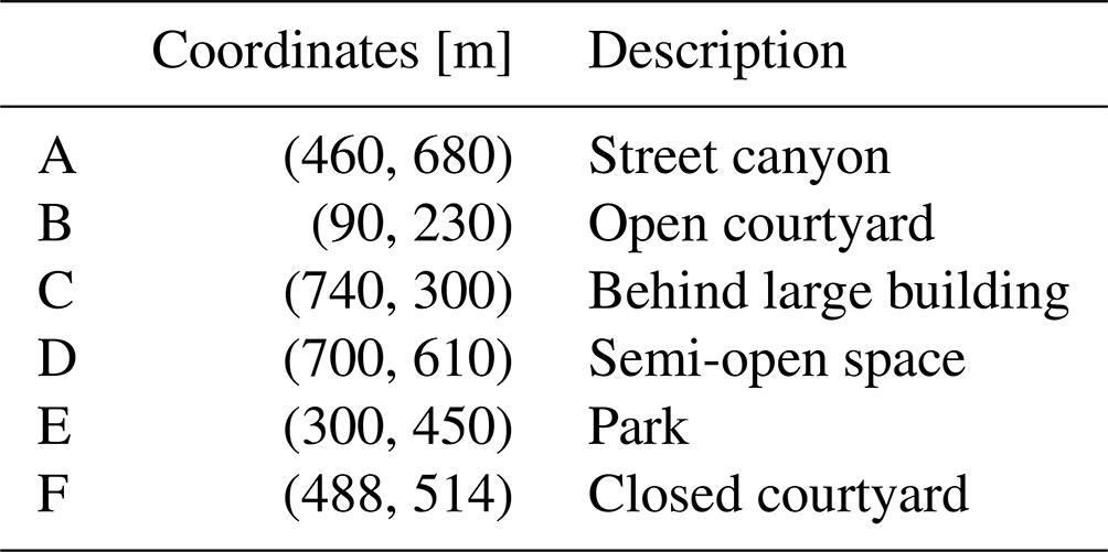
The simulation has been set up for 48 h, starting on 00:00:00 UTC on 5 January 2022, preceded by a 6 h spin-up period. Sampling takes place in the final 24 h. The model run was performed on the HLRN supercomputer system described in Sect. 3.3 on 20 × 20 compute cores. Time-averaged 3D output data (over a 5 min window) for all relevant prognostic variables were written out at 5 min intervals. Six sampling locations, representing various types of urban topology, have been selected from the domain. Sampling location A represents a typical street canyon, where two long rows of buildings are separated by a narrow road segment. Location B is situated in an open courtyard, i.e., an open area surrounded by buildings. The region immediately downwind of a large building is indicated in sampling location C, while a heavily built-up area but with an open downwind region is represented by location D. Sampling location E is an open space in the middle of a park. Finally, sampling location F is a completely closed courtyard. These locations are visually indicated in Fig. 7 and tabulated in Table 4.

Table 4 Sampling locations in the computational domain (Fig. 5). Easting and northing coordinate values are relative to the domain origin (52°32^′32.6^′′ N, 13°23^′46.5^′′ E).

4.1 Temperature deficit

To evaluate the behavior of the domestic heating parametrization throughout the idealized model run, the hourly mean nominal domain temperature deficit ΔT(t) as well as the weighted deficit with the CAMS diurnal profile ζΔT(t) are presented in Fig. 6. The temperature deficit varies with the ambient temperature. It begins at 00:00 UTC at 15.55 °C and increases monotonically, albeit slowly, to 15.78 °C at 07:00 UTC. Rapid changes follow in which the ΔT(t) drops to 7.89 °C at 12:00 UTC and then returning to 13.6 °C at 16:00 UTC. The end of the day sees a mild increase, where ΔT(t) returns to 15.50 °C towards the end. As ΔT(t) is positive throughout the day, the domestic stacks should be continuously operating and emitting PM₁₀, in accordance with Eq. (9).

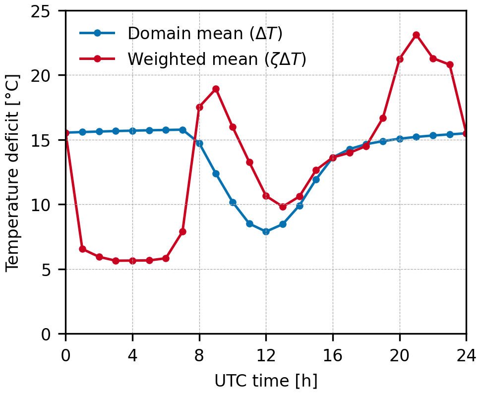
Figure 6 Domain hourly mean for temperature deficit (blue) and hourly temperature deficit weighted by CAMS diurnal profile (red) for residential and commercial combustion (obtained under GNFR sector C).

On the other hand, the weighted temperature deficit ζΔT(t), which exhibits a different behavior than the nominal ΔT(t), reflects the influence in meteorological conditions as well as anthropogenic activities on the expected energy usage and the corresponding emission level, as indicated in Eq. (7). Domestic heating is expected to be reduced substantially in the nocturnal period from 01:00 to 06:00 UTC, when the majority of residents are at rest, and the weighted temperature deficit hovers between 6.55 °C (01:00 UTC) and 5.64 °C (03:00 UTC). The morning peak takes place at 09:00 UTC, with an onset starting at 08:00 UTC where ζΔT(t) equals 18.9 °C but quickly reduces to 9.82 °C at 13:00 UTC due to the corresponding decrease in ΔT(t) in the daytime period. A steady recovery period follows, in which ζΔT(t) rises to its evening peak value of 23.13 °C, reflecting a generally high level anthropogenic activity, before dropping quickly to 15.50 °C at 00:00 UTC. While it is impractical to draw trends from inspecting the output of all stacks due to variability in energy demands and local meteorology, the weighted temperature deficit serves as a reasonable indicator for their overall level of operation and by extension their emission characteristics.

4.2 Spatial distribution of PM₁₀ concentration fields

Figure 7 shows the spatial distribution of diurnal mean PM₁₀ concentration evaluated at 2 m above ground. As expected, higher PM₁₀ concentrations can be found in the wake of building clusters due to the release of pollutants from the stacks. These can range from approximately 2 to above 4 µg m⁻³, depending on the location. On the other hand, in open areas, where stack exhaust disperses into its surroundings, lower concentrations can be seen, ranging about 1–1.5 µg m⁻³. This range of modeled concentration levels is in good agreement with the observed contributions of domestic heating of PM₁₀ concentrations found in existing studies for Berlin (Senatsverwaltung Berlin, 2019; Pültz et al., 2023).

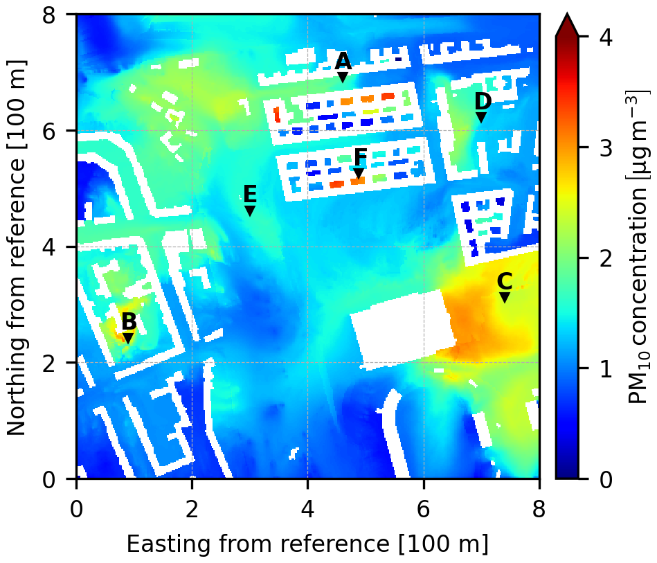
Figure 7 Horizontal spatial distribution of diurnal mean PM₁₀ concentration evaluated at 2 m above ground, with markers indicating positions of sampling locations listed in Table 4.

The magnitude of the concentration also corresponds to the energy consumption (E_B) of the individual buildings, which depends on their volume and footprint according to Eq. (8). Thus, it can be seen that concentrations of PM₁₀ are higher following the wake of larger buildings (e.g., at locations B, C, and D). On the other hand, pollutant accumulation can be seen at locations where pollutant transport between the urban canopy and the free stream is restricted through the turbulent shear layer (Chan and Butler, 2021). Regions such as the street canyon (location A) as well as the closed courtyard (location F) are exemplary of such pollutant accumulation. Particularly, the vicinity of location F contains a large number of stacks (Fig. 5), which results in a large amount of local PM₁₀ being trapped in individual courtyards. In other cases, pollutants are transported from nearby buildings, in addition to local emission production, as qualitatively evidenced in the street canyon at location A.

4.3 Concentrations at sampling locations

The diurnal time series for the PM₁₀ concentrations at 2 m above ground for each sampling location is illustrated in Fig. 8, in which they follow a general trend. The concentrations reported from the idealized run are relatively low for all locations, with mean values between 1.65 and 3.11 µg m⁻³ for each location. Higher concentrations can be observed towards the beginning and end of the day, separated by a period during daytime, starting at 09:00 UTC, when the concentration is very low, averaging between 0.30 and 1.64 µg m⁻³. As most locations (A to E) are positioned at some distance away from the emission sources at rooftop levels, the low concentrations indicate dilution through daytime vertical transport. This is not surprising, considering that the prescribed wind for this idealized run is constant but low. Meanwhile, there is very weak dispersion during nighttime (from 00:00 to 08:00 UTC), which only causes the concentrations at all stations to decrease very slowly. The concentration recovers more quickly in the evening, coinciding with an increase in ζΔT(t), with the exception of locations C and F, where the recovery begins at 16:00 UTC.

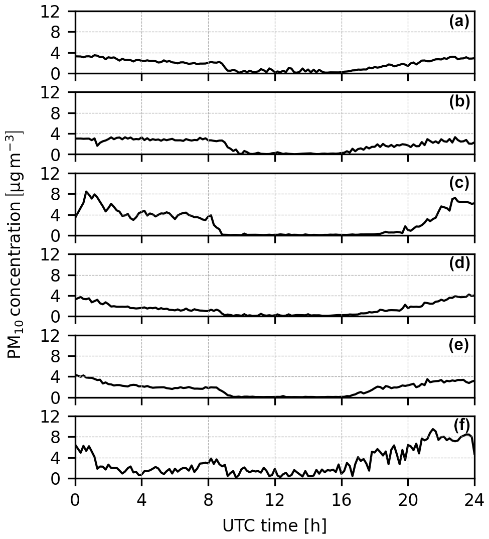
Figure 8 Diurnal time series for PM₁₀ concentrations at 2 m above ground for each sampling location.

Location C is downstream of an isolated large emission source. Therefore, it maintains a higher peak concentration than the other stations, at 8.42 µg m⁻³. On the other hand, without other emission sources in its proximity, the concentration at location C also takes longer to recover than at the other locations, at 19:00 UTC, but the concentration rises quickly to its evening peak (8.42 µg m⁻³). By comparison, location F is in a closed courtyard in a large building complex. With numerous emission sources in its surroundings, a relatively high amount of PM₁₀ finds its way into the courtyard. However, pollutant exchange with the free stream flow is restricted through the rooftop shear layer (Chan and Butler, 2021), effectively trapping the PM₁₀ inside the courtyard. This results in a steady increase in PM₁₀ concentration in the evening to a peak of 9.49 µg m⁻³. Following a sharp decrease at 01:20 UTC, corresponding to a decrease in anthropogenic activities, the concentration maintains a relatively constant level throughout the day, with a mean of 1.53 µg m⁻³ between 02:00 and 16:00 UTC.

Since domestic emissions are released from rooftops, further insights can be obtained by inspecting the vertical profiles of PM₁₀ concentrations at each sampling location, as illustrated in Fig. 9. The profiles at four different points in time (08:00, 12:00, 16:00, and 20:00 UTC) are shown, representing the morning peak, daytime low, onset of recovery, and evening peak, respectively. Due to the vertical positioning of the domestic stacks, PM₁₀ must be transported downwards to the ground level, which implies that lower concentrations are expected than those further up in the urban canopy, even in cases where the distribution is seemingly uniform (i.e., location F).

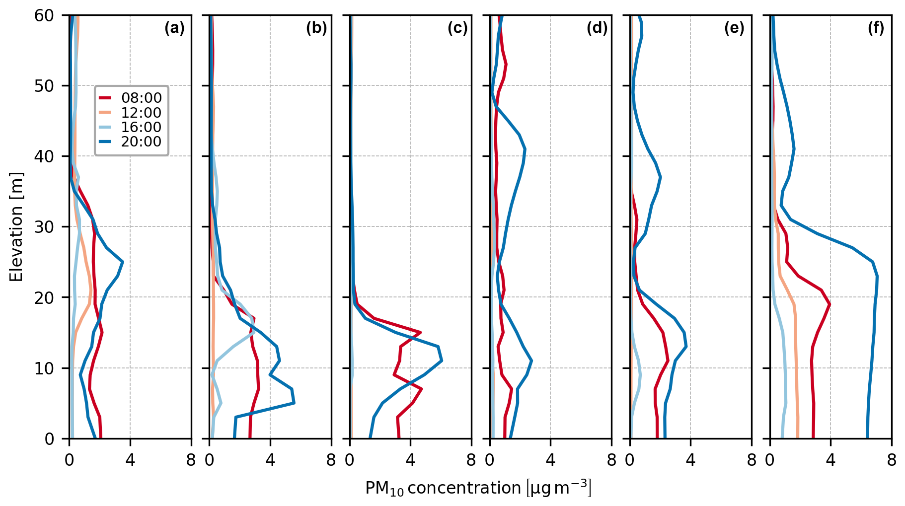
Figure 9 Diurnal mean vertical profiles for PM₁₀ concentrations above ground level for each monitoring location.

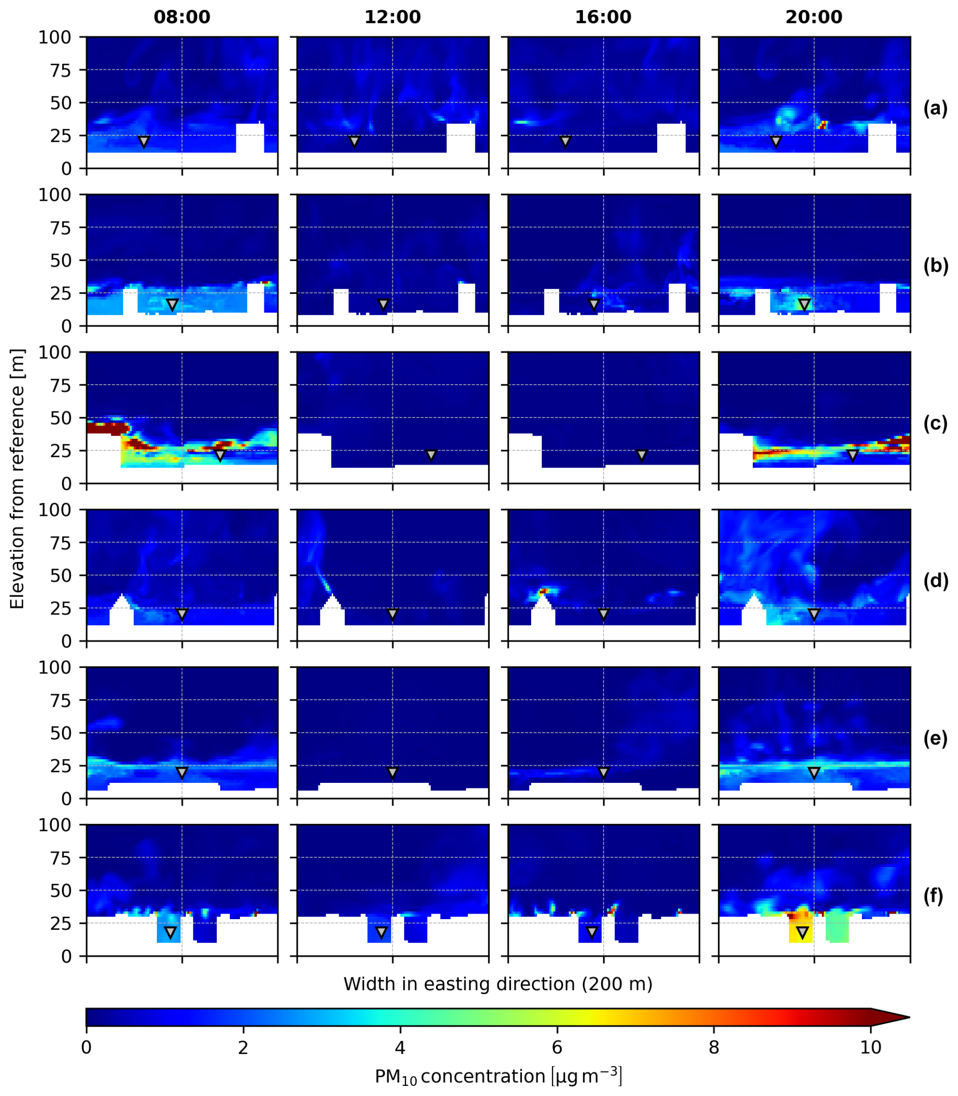
Figure 10 Vertical cross sections of PM₁₀ concentration in the vicinity of each sampling location at 08:00, 12:00, 16:00, and 20:00 UTC. The sampling plane is taken at the north–south position of each location. The east–west direction of each figure covers a distance of 200 m. Triangular markers indicate positions of the sampling locations. Elevations are relative to a reference value of 36.87 m above sea level.

The concentration profiles themselves are also indicative of the urban topology of the corresponding sampling locations. Location A is a typical street canyon, and a relatively stable vertical concentration profile can be found at all times. The canyon is well ventilated due to alignment of the road section with the wind flow. This results in a uniform vertical distribution of PM₁₀ concentration along and beyond the building height of 22 m on both sides of the canyon, with a mean of between 0.32 µg m⁻³ at 16:00 UTC and 1.80 µg m⁻³ at 20:00 UTC, up to an elevation of 30 m above ground. As indicated in the diurnal mean concentrations in Fig. 4, such a stable distribution can be brought about by the emissions from the cluster of buildings about 300 m upstream from location A, as well as stacks from nearby buildings.

In contrast, location B is located in a cluster of buildings, and as such the vertical PM₁₀ concentration is dominated by emissions of local sources. It is also more vertically stratified than location A. There is a higher uniformity at 08:00 UTC, averaging 2.62 µg m⁻³ up to the building height of 22 m, before diminishing near the rooftop. This indicates mixing of the PM₁₀ that remains from the previous evening, which is almost completely dissipated by 12:00 UTC. At the onset of recovery (16:00 UTC), a peak of 2.92 µg m⁻³ can be seen developing from the roof and being transported to ground level, as evidenced by the profile at 20:00 UTC, when peak concentration reaches 5.57 µg m⁻³ while downward transport still takes place.

As previously mentioned, the concentration at location C is highly dependent on a single, large emission source located 185 m upstream. Therefore, while the concentrations could be significant, vertical mixing could be relatively weak, particularly due to the absence of other urban structures along the way to provide turbulence mixing and additional emission sources. This single source can thus provide a level of concentration comparable to the other locations, up to 4.72 µg m⁻³ at the morning peak (08:00 UTC) and 6.05 µg m⁻³ at the evening peak (20:00 UTC). However, for this reason it is also more vertically stratified. Furthermore, at periods of low daytime emissions – indicated by ζΔT(t) in Fig. 6 – the PM₁₀ is seen to be totally dispersed before reaching location C.

Location D is situated in a similar topology as location B, where it is an open area surrounded by many buildings, with the exception of a cluster of nearby buildings upwind, which also serves as a rich source of PM₁₀, as shown in Fig. 5, particularly during the evening peak. Therefore, this contributes to the presence of uniform PM₁₀ even at higher elevations, up to 2.32 µg m⁻³ at 20:00 UTC. However, this uniformity is not maintained at the other points in time, suggesting the magnitude of emission as being the primary driver for vertical transport. A similar observation can also be made for locations E and F, in which there are also numerous sources in their vicinity.

Despite being in a completely open area, the concentrations at location E are at a similar level as the other sampling locations, with maximum values of 2.51 µg m⁻³ at 08:00 UTC and 3.71 µg m⁻³ at 20:00 UTC. There is a strong dependence on contributions from nearby sources found in the building clusters at some distance upwind, as with location C. However, the PM₁₀ also diminishes quickly during periods of relatively low emission levels (12:00 and 16:00 UTC) through dispersion.

The restriction of pollutant exchange at location F, compared to the other locations, has been prominently discussed in the previous paragraphs. The direct consequence of this is the accumulation of PM₁₀, which results in a highly uniform vertical distribution at relatively high concentrations, with mean values ranging from 0.640 µg m⁻³ at 16:00 UTC to 6.40 µg m⁻³ at 20:00 UTC, up to the building height of 30 m. Mixing at higher altitudes is also evident, indicative of the contributions from numerous nearby emission sources upstream, as pointed out previously for locations D and E.

A qualitative representation of PM₁₀ dispersion can be seen in Fig. 10. It shows the vertical distribution of PM₁₀ concentrations at each sampling location, indicated with triangular markers, from 08:00 to 20:00 UTC at 4 h intervals. The sampling plane is taken at the north–south position of the corresponding location, spanning a width of 200 m in the east–west direction and covering an elevation of 100 m from the reference height. The higher concentrations during peak periods have been discussed in Fig. 9. Vertical transport is also evident in each of the regions, albeit heavily attenuated during off-peak times (12:00 and 16:00 UTC). The uniformity of the PM₁₀ concentration inside the urban canopy can be seen at location B at 08:00 UTC, as well as at location F at 20:00 UTC. The distribution plots provide a visual confirmation of the conclusions drawn from the previous figures. For instance, the much higher concentrations at the stack upstream of location C, which have been discussed previously, are clearly seen at 08:00 and 20:00 UTC. Moreover, contributions from nearby emissions can be observed at locations D and E, where relatively high levels of PM₁₀ reach the sampling location from above, especially at 08:00 UTC. It is worth noting that the urban structures are not necessarily contained with the corresponding sampling planes. As such, the figures may capture emissions from nearby sources that do not appear in the figures. As such, the figures show local concentration maxima originating from nearby sources, which are located outside the area indicated in the figures.

5 Concluding remarks

An enhanced emission module has been developed for the PALM model system to provide a homogeneous operating framework for modeling emission contributions from various emission sectors at different levels of detail (LODs) and parametrizations. The hash key approach allows references from individual emission sectors to be made directly to the prognostic equation source terms in a highly effective and independent manner. In the mean time, modular interface functions and subroutines are provided to ascertain operational uniformity across all emission sectors with the PALM model system core, while encapsulating internal data and methods for each emission module and the framework itself. A benchmark run showed excellent performance and scalability.

A module for domestic heating emission parametrization, based on the work of Baumbach et al. (2010) and Struschka and Li (2019) was implemented using the enhanced emission framework. The parametrization relates emissions to energy demand of each individual building, which is driven by the building topology and the deficit between the ambient temperature and the target indoor temperature, weighted by the diurnal variation in domestic heat usage. In addition, the stack emission outputs were influenced by predetermined tabulated factors for different building types and age, as well as emission factors for different pollutants and furnace technologies, which are used in the parametrized module as default values.

Subsequently, a test case under idealized conditions was conducted for the parametrization module over a 800 × 800 m² residential region in Berlin. The model run covers a 24 h sampling period following spin-up under constant wind and surface temperature. The diurnal time series for nominal (ΔT(t)) and weighted (ζΔT(t)) temperature deficit reflect continuous furnace operation with highly varying energy usage and emission output throughout the day, showing a short daytime peak and a longer evening peak. Near-surface PM₁₀ concentrations at different sampling locations show similar trends, showing very low levels during daytime due to low levels of heating and dispersion through vertical transport. Meanwhile, values are persistently moderate during nighttime, following the evening peak. Vertical concentration distributions vary depending on the topology of each sampling location. It is shown that a large number of nearby emission sources heavily influence vertical distribution at elevations beyond building height, while the uniformity of the vertical column is dependent on the level of ventilation of the area surrounding each location.

The performance and functionalities of the new approach in the PALM model system have been fully demonstrated in the present work through the benchmark (Sect. 3.3) and the idealized run (Sect. 4). This approach to emission source treatment enables emission models for the PALM model system to be designed and developed in a highly intuitive, flexible, and independent manner. For the end user, the modularization of different emission sectors offers a higher degree of control over execution options and details, allowing studies to be conducted with improved organization and precision. The parametrization assumes uniform heating technology for all buildings in the computational domain, however. The emissions are further considered isothermal and well mixed in the cell directly above the building stack. These limitations can be partially addressed using either the LOD 2 specification or the built-in generic emission mode, which gives the user the ability to import third-party emission data.

In addition to the domestic emission parametrization module featured in this work, implementations of additional modules for the parametrization of biogenic VOC emissions, pollen dispersion, and E-PRTR or GRETA (Schneider et al., 2016) point sources are available from the most recent release (23.10) of the PALM model system at the time of writing. Further enhancements have been planned for the parametrized domestic emission module itself. These include building heat loss estimation and thermal effects on stack exhaust dispersion. Finally, a simplified characterization of ground-based emission sources (such as road traffic) can be represented as surface fluxes (Khan et al., 2021; Gehrke et al., 2021) within the present emission module framework.

Appendix A: Nomenclature

A1 Roman symbols

A	Annual aggregate (subscript)
B	Building index (subscript)
EB	Building energy consumption [kW h]
Eβ	Per footprint energy demand for building type β [kW h m−2 p.a.] (p.a. is per annum)
f	Parametrized emission source function in Eqs. (4) and (10)
H	Amalgamated global hash map
hm	Hash map for emission sector m
$i,j,k$	Cell indices
m	Emission sector index (superscript)
n	Sample size in Eq. (11)
N	Array size
p	Index for pollutant species (subscript)
r	Index for chemical reaction (superscript)
s2	Unbiased sample variance estimator [⋅2]
T	Temperature [K]
T0	Base building temperature [K]
T∞	Ambient temperature [K]
ΔT	Temperature deficit [°C]
ΔTA	Annual heating degrees [°C]
t	Time [s]
u	Wind velocity [m s−1]
V	Building volume [m3]
W	Natural number ($\in \mathrm{0},\mathrm{1},\mathrm{2},\mathrm{\dots }$)

A2 Greek symbols

β	Building type index (subscript)
ϵ	Volumetric emission rate [m−3 s−1]
ζ	Diurnal weight factor for anthropogenic activity [ ]
η	Generalized parameter in Eq. (4)
Γ	Species diffusivity [m2 s−1]
κ	Hash key
ξ	Pollutant concentration [⋅ m−3]
σ	Chemical production rate [m−3 s−1]
Φ	Building compactness factor [m−1]
Ψ	Emission factor [mol TJ−1] or [kg TJ−1]

A3 Acronyms and abbreviations

CAMS	Copernicus Atmosphere Monitoring Service
DOF	Degrees of freedom
E-PRTR	European Pollutant Release and Transfer Register
(G)NFR	(Gridded) nomenclature for reporting
GRETA	Gridding Emission Tool for ArcGIS
HDD	Heating degree day
HLRN	Norddeutscher Verbund für Hoch- und Höchstleistungsrechnen
KPP	Kinetic preprocessor (Damian et al., 2002)
LES	Large eddy simulation
LOD	Level of detail
PM10	Particulate matter with mean diameter of up to 10 µm
VOC	Volatile organic compound

Appendix B: Building-specific parameters for domestic heating emissions

Six building types are supported in the current implementation of the parametrized domestic heating emission sector, based on their function and construction period, to represent their energy consumption characteristics shown in Table B1.

Each building type (β) is further defined by its compactness factor (Φ_β) and annual energy demand (E_β). The following results are taken from Struschka and Li (2019) and are presented in Table B2 below.

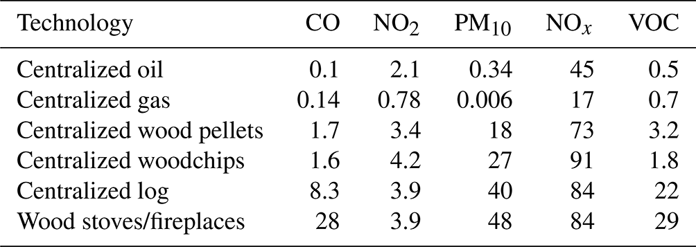
Furthermore, Struschka and Li (2019) have also proposed emission factors for carbon monoxide (CO), oxides of nitrogen (NO_x and NO₂), particulate matter (PM₁₀), and volatile organic compounds (VOC). These values have been tabulated in the table below according to each domestic furnace technology (Table B3). Please note that the emission factors used for the idealized run in Sect. 4 are taken as the arithmetic mean between centralized oil and centralized gas to reflect the furnace technology composition of the region of interest (Senatsverwaltung Berlin, 2010).

Table B1 Building type (β) definitions.

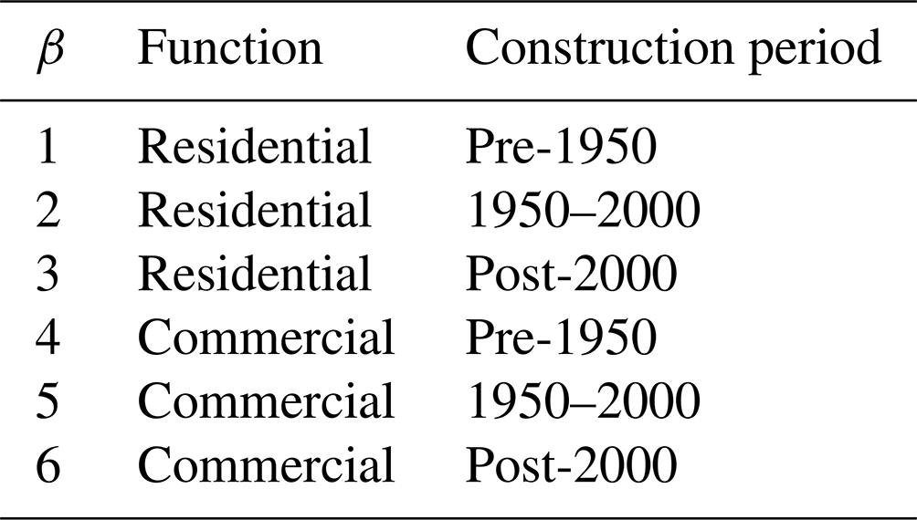
Table B2 Compactness factor (Φ_β) and annual energy demand (E_β) for each building type (β). Φ_β is in units of m⁻¹, while E_β is in units of kW h m⁻² per annum.

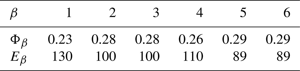
Table B3 Emission factors for major pollutant species for different domestic furnace technologies. CO and NO₂ are in units of mol TJ⁻¹, while PM₁₀, NO_x, and VOC are in kg TJ⁻¹.

Appendix C: Namelist parameters for the exemplary model run

The following namelist options are used for the chemistry parameters in the idealized domestic model run described in Sect. 4. Settings relevant to the parametrized domestic emission module all begin with emis_domestic_ and are further explained. The reader may refer to Khan et al. (2021) for infirmation on the remaining options pertaining to the PALM chemistry module. Instructions for obtaining the complete namelist and all associated input data can be found in the “Code and data availability” section.

&chemistry_parameters
  chem_gasphase_on          = .TRUE.,
  call_chem_at_all_substeps = .FALSE.,
  chem_mechanism            = 'phstatp',
  photolysis_scheme         = 'simple',
  surface_csflux_name       = 'PM10',
  surface_csflux            = 0,
  cs_name         = 'PM10',
  cs_surface      = 0,
  cs_heights(1,:) = 0,50,100,200,400,800,
  cs_profile(1,:) = 0, 0,  0,  0,  0,  0,
  bc_cs_l  = 'dirichlet',
  bc_cs_r  = 'neumann',
  bc_cs_s  = 'dirichlet',
  bc_cs_n  = 'neumann',
  bc_cs_b  = 'neumann',
  bc_cs_t  = 'neumann',
  emis_domestic                              = .TRUE.,
  emis_domestic_lod                          = 0,
  emis_domestic_species_names(:)             = 'PM10',
  emis_domestic_species_emission_factors(:)  = 0.173,
/

The domestic emission module is activated by setting the flag emis_domestic to .TRUE.. By setting the value of emis_domestic_lod to 0, the module utilizes the full parametrization option described in Sect. 3. All modeled emitted species, as well as their corresponding emission factors, can be specified using the namelist parameters emis_domestic_species_names and emis_domestic_species_emission_factors, respectively. For this run, the emission factor for PM₁₀ is 0.173 kg TJ⁻¹, representing an equal contribution of centralized oil and centralized gas for all buildings shown in Table B3. Any species not present in the active mechanism will be ignored.

The following parameters are absent from the namelist, where default values are assumed:

  emis_domestic_update_interval =  300,
  emis_domestic_heating_degree  = 2100,
  emis_base_temperature         =   15,
  emis_domestic_compact_factors = &
      0.23, 0.28, 0.28, 0.26, 0.29, 0.29,
  emis_domestic_energy_demands  = &
      130, 100, 100, 110, 89, 89,

The parametrization is updated every 300 s of simulation time, as indicated by emis_domestic_update_interval. The values of emis_domestic_heating_degree and emis_domestic_base_temperature represent the corresponding annual heating degree and the target outdoor temperature (both in °C) of each building. The parameters emis_domestic_compact_factors and emis_domestic_energy_demands, when unmodified, adopt respective values and units listed in Table B2 in the order of the building types presented in Table B1.

In addition, the parametrized domestic emission model requires data on the type (Table B1) and volume of each building in the computation domain, as well as the corresponding stack location. This information is located in the model _static file (Sect. 3.2). The variable stack_building_volume contains the volume of each building at the building stack location, while building_type, as its name suggests, defines the type of each building.