Robust handling of extremes in quantile mapping – “Murder your darlings”

Quantile mapping is a method often used for the bias adjustment of climate model data toward a reference, i.e. to construct a transformation of the model's distribution to that of the reference. The main moments of the distributions are typically well transformed by quantile mapping, but statistical uncertainty increases towards the extreme tails, making robust transformations challenging. Because of the limited data at the extreme tails, an empirical quantile mapping also needs to make some estimation or fit a parameterised function for data beyond the calibration data range. Here, the MIdAS bias adjustment platform is employed to explore different methods for handling the extreme tail; these approaches are evaluated using an indicator of extreme precipitation – the maximum daily precipitation amount per year. Different methodologies are evaluated for a large ensemble of regional climate model projections over Scandinavia. The sensitivity of the empirical quantile mapping to the tails of the distribution is demonstrated, and it is found that the behaviour is significantly different within and outside of the calibration period, causing severe issues with the temporal consistency of the time series. The sensitivity is identified to be due to differences in the activated features of the bias adjustment within the calibration period (where the empirical transfer function is applied) and outside of that period (where the extrapolation method is likely applied). This means that the bias adjustment method is, in a sense, different between different time periods. Furthermore, finding a robust parameterisation for the tail is not straightforward. We identify a two-step solution that works well for this problem:

1. We refer to the first step as “Murder your darlings”. By excluding data from the tail data in the calibration period, the extrapolation feature is activated for all time periods, even the calibration period.

2. In the second step, applying an outlier-insensitive method for linear regression works well for finding an extrapolation parameterisation for the tail.

1 Introduction

Bias-adjusted climate projections are routinely used for impact modelling and are further processed into climate indicators for various climate services. Climate indicators of extremes are, by definition, sensitive to small samples; they become even more sensitive when combined with the reference data used to map a transformation in the bias adjustment step. Such sensitivity can impose large uncertainties in the interpretation and conclusions drawn from an extreme indicator, in the worst case rendering the information useless or even misleading.

Many bias adjustment methods are based on the quantile mapping approach, in which a transfer function is used to map model data in different quantiles of a distribution to match that of the reference data set (see further detailed descriptions in Berg et al., 2022). Earlier studies have identified issues with bias adjusting data outside of the calibration range for pure empirical quantile mapping approaches (Boé et al., 2007; Bellprat et al., 2013). A common solution is to apply the adjustment value of the high end of the calibration period for all data outside of the calibration range (Themeßl et al., 2011), although this may introduce unrealistically large adjustments (Switanek et al., 2017). A combination of empirical and parametric approaches have been proposed by several authors, such as the use of extreme value theory fits to the top 5 % of data (Tani and Gobiet, 2021), while others have applied linear fits to the extremes (Holthuijzen et al., 2022).

Clearly, a purely empirical method based on all data within the calibration period might act differently when applied outside of the calibration data range compared with its calibration. The method reacts to data outside of the calibration range differently to that inside the range, for example, reusing the highest adjustment value of the calibration range (Themeßl et al., 2011), which means that the behaviour of the bias adjustment differs depending on the magnitude of the values that are adjusted. In other words, the bias adjustment method differs for data within and outside of the calibration range. This may lead to unexpected results for the bias-adjusted tails. One can only force the bias adjustment to apply its full effect by making sacrifices at the very tail of the distribution. In a way similar to the literary method of “Murder your darlings” (Quiller-Couch, 2015), also known as “Kill your darlings”, i.e. to remove the most precious items for the greater good of the work, “Whenever you feel an impulse to perpetrate a piece of exceptionally fine writing, obey it – whole-heartedly – and delete it before sending your manuscript to press. Murder your darlings”.

This paper presents a clear example of the problematic side-effects of bias adjustment within and outside of the calibration period. A new method to handle the calibration strategy and distribution fits to the tail is presented and tuned to find a pragmatic use of data, while also reducing the side-effects. The example is based on data from the Swedish climate service, using a large ensemble of regional climate models and the MIdAS bias adjustment method (Berg et al., 2022).

2 Bias adjustment

The MIdAS implementation of quantile mapping starts from the quantile–quantile (Q–Q) plots of the reference and model data sets, which share the same number of data points. A piecewise linear smoothing spline function is fitted to the Q–Q plot (see Berg et al., 2022, for details). MIdAS applies a linear function fitted to the 90 % most central data points of the Q–Q plot, with weights defined by the standard deviation of the data points from the linear fit. A linear continuation of the spline is applied to data points outside of the calibration data range, i.e. a “one-to-one” linear continuation of the spline in the Q–Q plot, as explained in detail in Berg et al. (2022).

The transfer functions are calculated based on a historical period, here 1971–2000, for each grid point and in subsets of the annual cycle. Rather than using calendar month subsets, as in most published methods, MIdAS is set up to calculate and apply the transfer functions based on the day of the year ($\mathrm{doy}=[\mathrm{1},\mathrm{365}]$), using a moving window of 15 d before and after the doy, such that 31 d multiplied by the number of calibration years is used to build the distribution of the reference and model data.

2.1 New parameterisation for the tail

The new development to handle data at the tails of the distributions is based on the Theil–Sen fitting procedure (Theil, 1950; Sen, 1968), which is an outlier-insensitive method. The procedure involves calculating the median of slopes derived from each individual pair of points in the sample, i.e. in the Q–Q plot. This means that outliers will have little individual effect on the fits, making the linear fits robust to the high sample uncertainties that are unavoidable at the tail of the distributions. The Theil–Sen approach aligns with the general philosophy of MIdAS, which is to use generally applicable methods that are not dependent on specific distributions. The reason for this philosophy is that MIdAS should be transparent and equally applicable across geographic regions and climates without the need to predefine specific distribution functions for each case.

When excluding high extreme data points in the calibration sample of precipitation, in order to activate extrapolation behaviour, and the full bias adjustment method, there are unavoidable effects on other moments of the distribution. Because precipitation extremes often add significant quantities of precipitation, they are important for defining the mean moment. Therefore, a balance between good handling of extremes and good adjustment of the mean moment must be found.

Different versions of excluding data from the calibration data range are combined with the Theil–Sen regression on the top 5 % of data to find a balance between side-effects on the tail data and, with a higher priority, the mean moment of the bias-adjusted data. These versions are as follows:

• R0T5 – no data exclusion and calibrate on percentiles 95–100;

• R1T5 – exclude 1 % of the data on the upper tail and calibrate on percentiles 94–99;

• R5T5 – exclude 5 % on the upper end and calibrate on percentiles 90–95.

2.2 Data

Precipitation data from SMHIGridClim (Andersson et al., 2021) are used as reference data for the bias adjustment. SMHIGridClim is a data set based on the UERRA regional reanalysis (UERRA, 2019) combined with gauge data from Sweden and neighbouring countries, mapped on a 2.5 km grid with a daily temporal resolution. For this analysis, the data set is conservatively remapped (using first-order conservative remapping following Jones, 1998) to the EURO-CORDEX 0.11° (approximately 12.5 km) grid covering Scandinavia.

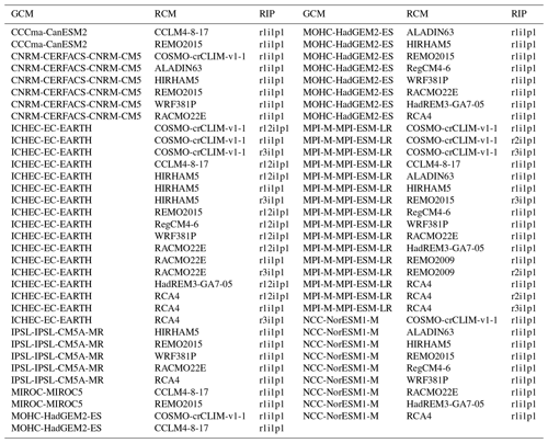
The climate projections are acquired from the EURO-CORDEX Coupled Model Intercomparison Project Phase 5 (CMIP5) data set (Jacob et al., 2020). A large ensemble of 67 unique combinations of global climate models (GCMs) and regional climate models (RCMs) are used (see Table 1), employing the RCP8.5 scenario of future emissions. The ensemble members all have bias to a different extent, for both the mean and the extreme tails, as evaluated for a subset of the ensemble in publications such as Vautard et al. (2021).

Table 1 List of the EURO-CORDEX GCM–RCM simulations included in the evaluation and the RIP (realisation–initialisation–physics) code.

2.3 Evaluation methods

Two statistics are used to evaluate the different methods in Sect. 2.1: the annual sum and the annual maximum of daily precipitation. The sum is evaluated because it summarises the performance of the bias adjustment across all data, while the annual maximum highlights the most extreme values, which are specifically targeted in this study. As the signal-to-noise levels are very high for the annual maxima, the ensemble mean is calculated across all members; in addition, a spatial average is calculated over the land regions of the complete domain. The figures present the temporal evolution of the ensemble mean for the domain-averaged annual sum and maxima.

3 Results

Figure 1 shows the performance of the different MIdAS setups for the annual maxima. The original MIdAS code is close to the reference data, which is expected as all of the data points are included, and the deviations for different ensemble members are due to how well the spline is fitted to the tail of the distribution. The different Theil–Sen methods show similar behaviour across the ensemble, although with a general underestimation of the annual maxima after bias adjustment. The remaining bias is on the order of less than 1 mm d⁻¹ for the mean of the ensemble, which is less than a 0.5 % relative bias. We consider this a sufficiently good fit, which does not indicate the need for more advanced fitting methods using extreme value theory.

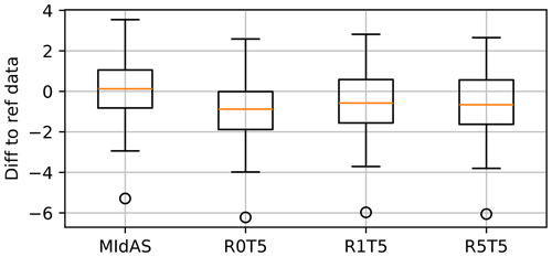
Figure 1 Remaining bias in the annual precipitation maxima (mm d⁻¹) for the ensemble members, presented as a box plot. Results are shown for the original MIdAS code and the different experiments.

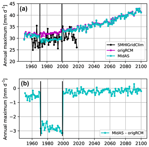
Figure 2 Annual precipitation maxima (mm d⁻¹) for SMHIGridClim, the original RCM ensemble mean, and the bias-adjusted data using the standard MIdAS setup for (a) absolute levels and (b) the difference between the bias-adjusted and original model data.

Figure 2 shows the original ensemble result of the annual maxima of daily precipitation averaged over the domain as well as the reference data and the resulting bias-adjusted data using the original implementation of MIdAS, as presented in Berg et al. (2022). In the calibration period, marked with vertical bars, the bias adjustment efficiently offsets the annual maxima, causing it to be at a similar level to the reference. Note that the interannual variability is reduced in this presentation, due to the ensemble averaging performed for the model data. However, outside of the calibration period, there is almost no visible effect of the bias adjustment, resulting in significant discontinuities at the beginning and end of the calibration period. This is clearly an issue and is, as will be shown, caused by the essentially different bias adjustment methods within (without extrapolation) and outside (with extrapolation) of the calibration period. The issue is very clearly seen in Fig. 2 because of the averaging over a larger domain. When assessed for single grid points or smaller domains, the issues are hidden within the high noise levels inherent in this kind of extreme precipitation statistics. This highlights the need to quality control and evaluate bias adjustment across larger areas, even though the parameterisation and scale of the bias adjustment is intended for single grid points. Clearly, if the calibration period was also used as a historical reference period, the climate change signal would be exaggerated by almost 3 mm d⁻¹, which is about twice the signal from the original data at mid-century.

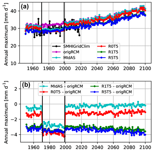
Figure 3 Same as Fig. 2 but with the additional data sets for the R0T5, R1T5, and R5T5 experiments. Note that the green line lies behind the blue line in panel (a).

In an attempt to improve on the performance outside of the calibration period, the Theil–Sen method is applied to find a good fit to the top 5 % of data in the distribution (experiment R0T5), which is shown as a red line in Fig. 3. The adjustment within the calibration period is only mildly affected, due to the change from an assumed linear extrapolation in the original MIdAS method and the Theil–Sen methodology. However, the main issue remains, as there is still a significant offset at the beginning and end of the calibration period.

Because the bias adjustment method will inevitably activate the extrapolation routine with data outside of the calibration range, the next experiments (R1T5 and R5T5) also force the extrapolation to be active within the calibration range. In other words, some extremes are excluded for the benefit of an overall better adjustment, at the likely cost of worse performance in the calibration period. Combining the Theil–Sen fit with exclusion of the top 5 % of the calibration data (R5T5, blue) has a strong impact on the bias across the whole time series. The bias is still well adjusted in the calibration period, equal to the R0T5 experiment, but with the additional much improved performance outside of the period. This result indicates that one can only reach a consistent bias adjustment across time periods by activating the extrapolation routine for all periods, which implies disregarding some tail data or in other words, “murdering your darlings”. Similar results are seen for experiment R1T5 (green), where fewer data (1 %) are excluded.

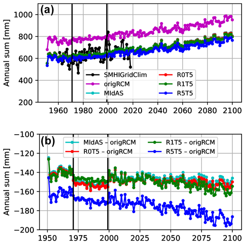
Figure 4 Same as Fig. 3 but for the annual sum of precipitation. Note that R0T5 is very close to R1T5 in panel (a).

So what are the side-effects? The annual maxima is but one of many important aspects that the bias adjustment is supposed to improve, and the more accumulated statistics, such as the mean values, are often more important to reproduce. Figure 4 shows the annual sums of precipitation, i.e. the result on the accumulated precipitation of all intensities. While the original MIdAS method works well for this measure, the R5T5 method clearly imposes a dry bias. This is because a significant amount of precipitation has been removed from the distribution in the calibration period (the 5 % of highest-intensity events), which strongly impacts the overall bias. The sign of this impact depends on the original bias in the mean and the maximum precipitation. They are likely of the same sign, as the maximum strongly affects the mean, but it may not always be that way. Reducing the exclusion of data to 1 % (R1T5), the annual sums are closer to the reference data set and the original method (Fig. 4) and, as presented above, still result in a similar result for the adjustment of the annual maxima (Fig. 3). However, Fig. 4 also highlights another important side-effect – a reduced trend in increasing precipitation with time – which is most clearly seen in the difference plot (Fig. 4b). This trend is seen for the original MIdAS adjustment and for all of the experiments, although the impact seems significantly stronger for experiment R5T5. No significant impact on trends in annual maxima is seen for the original MIdAS adjustment or experiment R0T5 (see Fig. 3b). However, when data are excluded in experiment R1T5 and R5T5, there is also an impact on the trends; this effect is very similar to that imposed on the mean statistic. One can debate between whether (1) this is a side-effect or (2) it is good to have consistent behaviour across the statistics, i.e. that the relative effects of the extremes and the means more closely follow each other in time.

4 Conclusions

This study focuses on an identified issue with bias adjustment of the highest extremes, which are adjusted differently within and outside of the calibration period. A new outlier-insensitive linear fit is used for the extreme tails, and a solution to the issue is presented using a set of experiments. The main conclusions of this work are as follows:

• The more extreme the statistic of interest is, the more elusive any bias becomes, as the available data become scarcer and the bias is a fundamentally statistical property. Therefore, to create a robust sample size, the bias should be assessed over an ensemble of simulations and/or over a larger set of grid cells.

• A consistent bias adjustment method must have all features activated across all time periods, including the calibration period, in order to produce consistent bias adjustment.

• The extrapolation feature can be activated by excluding the highest data points in the calibration period, thereby ensuring that the extrapolation feature is acting on the complete time range, resulting in consistent bias adjustment.

• An unavoidable trade-off between the adjustment of the mean moment and the extremes is necessary, as excluding high-intensity data points from the calibration will inevitably affect the mean.

• As there is an ever-increasing focus on climate extremes, we suggest that the performance assessment of bias adjustment methods should routinely include an examination of its impact on the extreme tails.