Experimental design for the Marine Ice Sheet–Ocean Model Intercomparison Project – phase 2 (MISOMIP2)

The Marine Ice Sheet–Ocean Model Intercomparison Project – phase 2 (MISOMIP2) is a natural progression of previous and ongoing model intercomparison exercises that have focused on the simulation of ice-sheet and ocean processes in Antarctica. The previous exercises motivate the move towards realistic configurations, as well as more diverse model parameters and resolutions. The main objective of MISOMIP2 is to investigate the performance of existing ocean and coupled ice-sheet–ocean models in a range of Antarctic environments through comparisons to observational data. We will assess the status of ice-sheet–ocean modelling as a community and identify common characteristics of models that are best able to capture observed features. As models are highly tuned based on present-day data, we will also compare their sensitivity to prescribed abrupt atmospheric perturbations leading to either very warm or slightly warmer ocean conditions compared to the present day. The approach of MISOMIP2 is to welcome contributions of models as they are, including global and regional configurations, but we request standardized variables and common grids for the outputs. We target the analysis at two specific regions, the Amundsen Sea and the Weddell Sea, since they describe two different ocean environments and have been relatively well observed compared to other areas of Antarctica. An observational “MIPkit” synthesizing existing ocean and ice-sheet observations for a common period is provided to evaluate ocean and ice-sheet models in these two regions.

1 Introduction

Model intercomparison projects (MIPs) for stand-alone ice-sheet models with floating ice shelves have been key to understanding what is needed in ice-sheet models to reproduce fast grounding-line migrations similar to those observed in West Antarctica (Pattyn, 2018). In particular, MISMIP (Marine Ice Sheet Model Intercomparison Project; Pattyn et al., 2012) and MISMIP3D (Pattyn et al., 2013), both conducted with idealized glacier geometries, highlighted the need for high (sub-kilometre) model resolution at the grounding line and the inclusion of membrane stresses. Recently, MISMIP+ (Asay-Davis et al., 2016) emphasized the improved agreement in model behaviours across a range of model architectures and the important role of ice-sheet sliding laws for a geometry representative of a highly buttressed ice shelf (Cornford et al., 2020). These MIPs have played a crucial role in the development of credible designs for Antarctic Ice Sheet projection frameworks (Nowicki et al., 2016).

The Ice Shelf–Ocean Model Intercomparison Project (ISOMIP; Holland et al., 2003; Hunter, 2006) was the first standardized configuration for stand-alone ocean models with a thermodynamically active ice-shelf cavity with fixed geometry (henceforth called ice-shelf–ocean models). However, ISOMIP has mostly been used as a test case for individual modelling groups (e.g. Losch, 2008; Gwyther et al., 2015; Mathiot et al., 2017). Its successor, ISOMIP+ (Asay-Davis et al., 2016), was implemented more as a coordinated intercomparison with a provided calibration method and common parameters. Results highlighted fundamental differences in simulated melt rates, depending on the vertical discretization and resolution of ocean models (Gwyther et al., 2020). When all the ocean models used the same physical parameters, the relationship between basal melt and the ocean circulation in the cavity was consistent across models, but the relationship did not hold when models were run with their typical parameter values (Xylar S. Asay-Davis et al., personal communication, 2024). This illustrates that despite facilitating the interpretation of an intercomparison exercise, the requirement of common set-ups may push the models far from their typical use, making it difficult to generalize the results for realistic configurations. The use of a single ice shelf in ISOMIP+ and the absence of realistic ocean–sea-ice dynamics over the continental shelf also made it difficult to generalize the melt sensitivity to the large variety of ice-shelf geometries in the whole Antarctic region (Jourdain et al., 2020; Burgard et al., 2022). Hence, previous MIPs motivate the move towards realistic configurations and more diverse model parameters and resolutions. One such approach was recently adopted by the Realistic Ice-shelf/ocean State Estimates (RISE) project in which the circum-Antarctic response of basal melting was evaluated against satellite-derived melt estimates in 10 circum-Antarctic ice-shelf–ocean models.

The continued development of ice-shelf–ocean models for Antarctica is a crucial step towards improved forecasts of sea-level rise and to further our understanding of the complex interactions between the ice sheet and other components of the climate system. However, so far, sea-level projections have relied heavily on the use of parameterizations of ocean-induced melt rates in stand-alone ice-sheet models. These parameterizations were identified as a major source of uncertainty in the Antarctic Ice-Sheet projections from the Ice Sheet Model Intercomparison Project for CMIP6 (ISMIP6; Nowicki et al., 2020; Seroussi et al., 2020; Payne et al., 2021; Seroussi et al., 2023). Since then, comparisons of these parameterizations to ice-shelf–ocean simulations have been used to better calibrate their sensitivity to ocean warming (Burgard et al., 2022; Reese et al., 2023; Jourdain et al., 2022). However, there is currently limited confidence in the validity of such ice-shelf–ocean simulations for several reasons: (1) important biases remain in the thermohaline structure and dynamical state of the ocean, in particular on the continental shelf; (2) the parameterizations for ice-shelf basal melt used in ocean models are highly tuned and structurally uncertain; and (3) no comprehensive comparison between model data and measurements of ocean properties and basal melt has been carried out. As such, the use of ice-shelf–ocean-model output to calibrate melt parameterizations that inform sea-level projections is questionable. A targeted ice-shelf–ocean MIP with a harmonized comparison of model output to available ocean data would help identify ocean-model similarities and differences, as well as better estimate uncertainties.

While melting parameterizations will undoubtedly remain useful due to their low computing cost compared to actual ocean models, they suffer from important biases despite improved calibration and increased complexity (Burgard et al., 2022). Therefore, many groups engaged in the development of coupled ice-sheet–ocean models, i.e. models in which the ice and ocean dynamics evolve together and feed back on each other (Thoma et al., 2015; De Rydt and Gudmundsson, 2016; Seroussi et al., 2017; Timmermann and Goeller, 2017; Goldberg et al., 2018; Favier et al., 2019; Pelle et al., 2021; Zhao et al., 2022; Pelletier et al., 2022; De Rydt and Naughten, 2024; Bett et al., 2024). While this type of coupling is emerging in Earth system models (Smith et al., 2021; Siahaan et al., 2022; Comeau et al., 2022), there is currently very limited knowledge on the fidelity of the simulated interactions. Similar to the case of stand-alone ocean models, a targeted MIP for coupled ice-sheet–ocean models would help identify some of these caveats and quantify uncertainties. The first Marine Ice Sheet–Ocean Model Intercomparison Project (MISOMIP1; Asay-Davis et al., 2016) was built along the lines of the aforementioned MISMIP+ and ISOMIP+, with a single idealized ice shelf and no interaction with atmosphere and sea ice. While MISOMIP1 has been useful for generating cohesion within the ocean and ice-sheet modelling communities and for beta-testing individual coupled models (e.g. Favier et al., 2019), progressing towards more diverse and realistic conditions would bring new information on the state of coupled ice-sheet–ocean modelling.

In this paper, we propose a protocol for MISOMIP2, a new coordinated intercomparison project for stand-alone ocean models representing ice-shelf cavities and for coupled ice-sheet–ocean models. While there previously were distinct names for ocean (ISOMIP+) and coupled (MISOMIP1) experiments, we now embed stand-alone and coupled experiments within a single acronym, MISOMIP2, for the sake of simplicity.

The first objective of MISOMIP2 is to investigate the robustness and biases of ice-shelf–ocean models (ocean models with fixed ice-shelf cavities) and ice-sheet–ocean models (ocean models with dynamically evolving cavities) in a range of Antarctic environments through comparisons to observational data that capture the range of natural ocean variability. The comparison to observations is not primarily designed to rank individual models, as targeted model tuning and bias compensations may hide poorly represented physical processes. Our aim is rather to assess the status of ice-sheet–ocean modelling as a community and, if possible, to identify common characteristics of models that are best able to capture observed features. For that reason, we have gathered a set of reprocessed observational products that can be used for MISOMIP2 or for individual model tests and calibrations. The corresponding observational database is referred to as the “MIPkit” in the following. As our objective is to understand differences between complex models, we will generally follow a “come-as-you-are” (CAYA) approach, with no prescription of model domain, resolution, physical parameters, and forcing.

Besides hindcast-type reference simulations, MISOMIP2 also includes a small number of perturbation experiments that are designed to deepen our understanding of model responses to a prescribed (large and abrupt) change in atmospheric conditions and to a prescribed change in cavity geometry. Importantly, we propose idealized perturbations to focus on strong changes over time windows compatible with a range of models of relatively high resolution and to have model responses that are relatively easy to interpret. The initial aim of MISOMIP2 is not to build scenario-based coupled ice-sheet–ocean projections, which is the remit of ISOMIP (Nowicki et al., 2016, 2020). The proposed model intercomparison will, however, contribute to improved future ice-sheet projections due to better constrained melting and freezing parameterizations and future climate simulations with interactive ice sheets thanks to a better understanding of the strengths and limitations of the various coupling approaches.

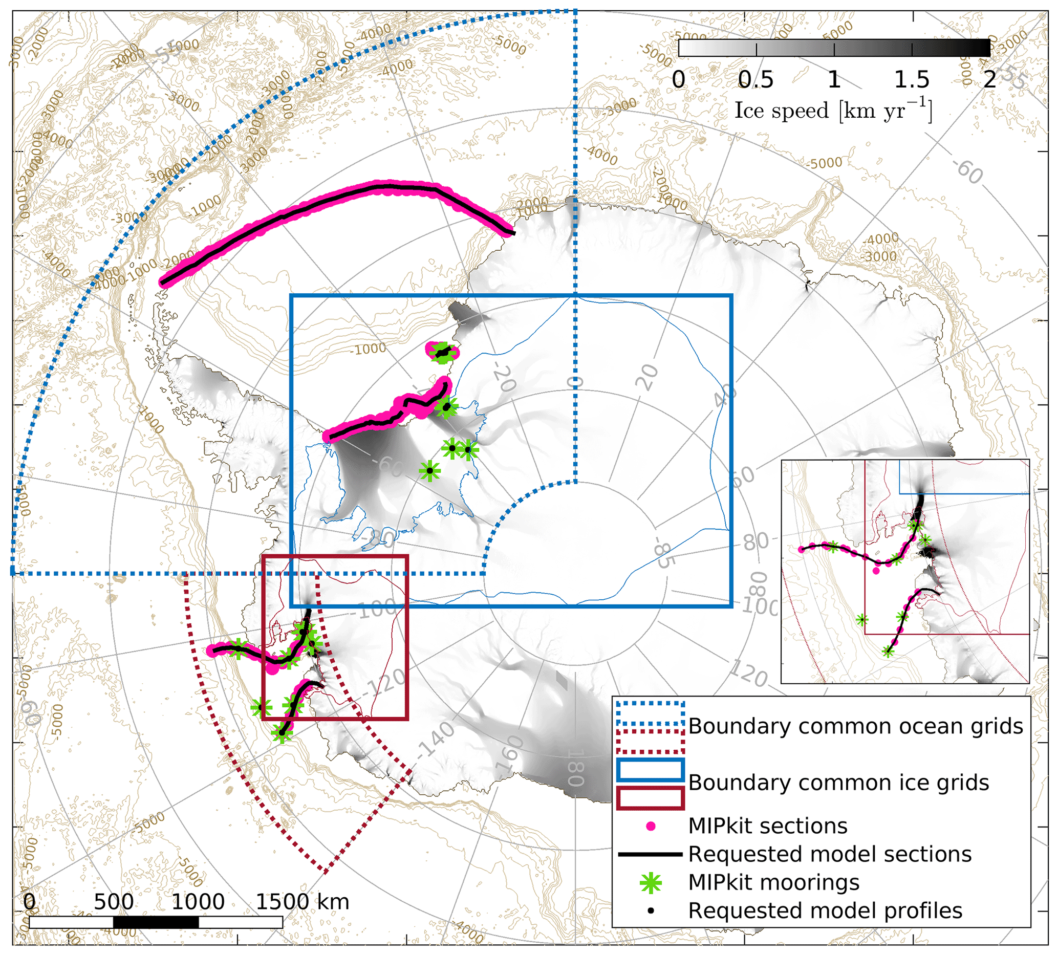
Figure 1 Boundaries of the standard MISOMIP2 grids for the ocean (dashed lines) and ice (solid lines) outputs of the Amundsen Sea (red lines) and Weddell Sea (blue lines) domains. Black lines indicate the locations of the requested model outputs along vertical sections (two in the Amundsen Sea and three in the Weddell Sea), as detailed in Sect. 4.1. Geographical locations of the conductivity, temperature, and depth and mooring data provided as part of the MIPkit are indicated by the green stars and pink dots, respectively. The inset above the legend provides a more detailed overview of the different section and mooring locations in the Amundsen Sea.

There will be two target regions in MISOMIP2, (1) the Amundsen Sea and (2) the Weddell Sea, and associated ice-sheet drainage basins, as illustrated in Fig. 1. These regions are chosen because they describe two contrasting present-day environments. Deep-water masses in the Amundsen Sea are relatively warm, with high ice-shelf basal melt rates driven by Circumpolar Deep Water that is found on the continental shelf (e.g. Jacobs et al., 2013; Dutrieux et al., 2014; Jenkins et al., 2018). The ice-sheet grounding zone has significantly retreated in recent decades (Rignot et al., 2014a; Scheuchl et al., 2016; Milillo et al., 2019, 2022), and there has been significant acceleration and mass loss of the grounded-ice sheet in this sector (Rignot et al., 2019; Shepherd et al., 2018). In contrast, the Weddell Sea is relatively cold, with associated low ice-shelf basal melt rates and refreezing beneath some parts of ice shelves due to strong ice-shelf thickness gradients and the presence of high-salinity shelf water on the continental shelf (e.g. Nicholls et al., 2009). The Filchner–Ronne Ice Shelf and the upstream ice sheet have remained relatively unchanged over the last few decades (Rignot et al., 2019), although future atmospheric perturbations may cause warm deep-water intrusions onto the continental shelf and initiate significant grounding-line retreat through enhanced basal melt (Timmermann and Hellmer, 2013; Hellmer et al., 2017; Timmermann and Goeller, 2017; Hazel and Stewart, 2020; Naughten et al., 2021). We would consider a good representation of these very distinct environments in a single configuration (or two analogous configurations of the same model) to be a good indication of model robustness. Moreover, a multi-decadal record of ocean data is available for both regions, with a more comprehensive coverage compared to other parts of the Southern Ocean, which facilities a more in-depth comparison between model results and observations.

In subsequent sections, we describe the experimental protocol for MISOMIP2, including the motivation and description of individual experiments (Sect. 2), a description of the datasets provided in the MIPkit (Sect. 3), and an overview of the requested model outputs (Sect. 4). To illustrate the experimental design, preliminary results from a range of global and regional ocean models and regional ice-sheet configurations are provided.

2 Experiments

2.1 Overview of the MIP experiments

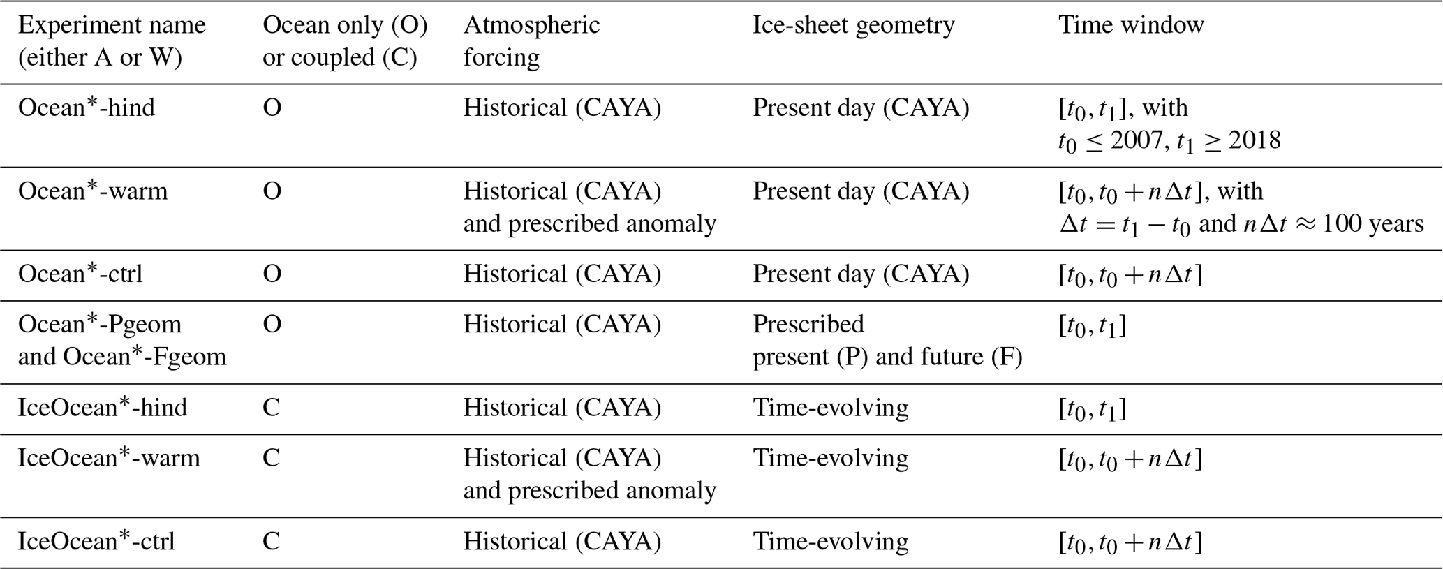
The MISOMIP2 experiments were designed with two broad objectives in mind. First, they were designed to test and intercompare the fidelity of ice-shelf–ocean models and ice-sheet–ocean models over the observational period, and second, they were designed to assess the sensitivity of models to a plausible change in the shape of the ice-shelf cavities and to a large perturbation in the atmospheric forcing. An overview of the experiments planned in MISOMIP2 and their time windows are provided in Table 1 and Fig. 2, respectively. Further details for each experiment are provided hereafter. In all the following, “A” stands for Amundsen and “W” for Weddell.

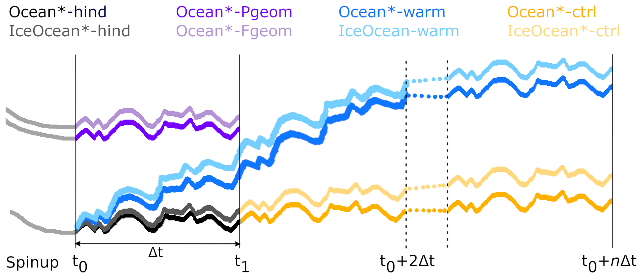
Figure 2 Schematic overview of the MISOMIP2 experiments and their respective time windows. As specified in more detail in Sect. 2, hindcast experiments (black and grey curves) and geometric perturbation experiments (purple curves) will cover the observational period between t₀≤2007 and t₁≥2018, with the exact time window decided by individual contributors. The atmospheric perturbation experiments (blue curves) and corresponding reference experiments (orange curves) start at time t₀ and end at time t₀+nΔt, where $\mathrm{\Delta }t=t_{\mathrm{1}}-t_{\mathrm{0}}$ and n are chosen to be sufficiently large, such that melt rates are equilibrated with the atmospheric perturbation (regional models) or nΔt≤100 years (global models).

Table 1 Overview of the MISOMIP2 experiments, where the asterisk (^*) is either A for the Amundsen domain or W for the Weddell domain. CAYA refers to “come as you are”. Further details are provided in Sect. 2.1 and 2.2.

• OceanA-hind and OceanW-hind experiments are designed to compare stand-alone ocean-model simulations with static ice shelves and present-day atmospheric forcing to a common set of ocean observations that are relevant to Antarctic ice shelves, to analyse multi-model sensitivity to external drivers, and to potentially identify clusters of models with a similar behaviour for specific modelling choices.

• OceanA-warm and OceanW-warm experiments are designed to compare the response of simulated melt rates to a transition to warm-ocean conditions in response to a rapid modification of the atmospheric forcing. The model configuration is otherwise identical to the OceanA-hind and OceanW-hind experiments. All models will apply a strong atmospheric perturbation representative of an abrupt shift to a warmer climate in the form of a prescribed anomaly to be added to the present-day forcing used in the OceanA-hind and OceanW-hind experiments. For regional models with open-ocean boundaries, an additional temperature and salinity anomaly is provided for the boundaries to represent the ocean warming outside the domain. A detailed description of the perturbations can be found in Sect. 2.3.

• OceanA-ctrl and OceanW-ctrl experiments are extensions of OceanA-hind and OceanW-hind forced by present-day atmospheric conditions to be used as a control for the perturbation experiments.

• OceanA-Pgeom/OceanA-Fgeom and OceanW-Pgeom/OceanW-Fgeom experiments are designed to compare the response of simulated melt rates in stand-alone ocean models to an imposed modification of the ice-shelf geometry. Two distinct geometries for the Amundsen Sea and Filchner–Ronne cavities are provided: one that represents the present-day state of the ice sheet (OceanA-Pgeom and OceanW-Pgeom experiments) and one hypothetical future state (OceanA-Fgeom and OceanW-Fgeom experiments). The atmospheric forcing remains unchanged between these experiments. The difference between the OceanA-Pgeom/OceanW-Pgeom and the OceanA-hind/OceanW-hind experiments is that in the former, the present-day geometry of the ice shelves is prescribed and provided as part of the MIPkit (see Sect. 3.3), whereas in the latter, the user is free to choose a present-day ice-sheet geometry as part of the CAYA approach. If participants choose to use the Ocean^*-Pgeom geometry for their Ocean^*-hind experiments, then both experiments will be identical, and results for only one experiment need to be submitted.

• IceOceanA-hind and IceOceanW-hind experiments are similar to OceanA-hind and OceanW-hind focusing on present-day conditions but with coupled ice-sheet–ocean models (including “intermediate-complexity coupling” through parameterizations; e.g. Kreuzer et al., 2021). Here we aim to compare the simulated ice and ocean evolution to recent observations. We will also attempt to estimate the change in bias (if any) that such coupled models attain compared to stand-alone ocean models.

• IceOceanA-warm and IceOceanW-warm experiments are designed to compare the response of the coupled system to the same idealized warm perturbation as for OceanA-warm and OceanW-warm.

• IceOceanA-ctrl and IceOceanW-ctrl experiments are extensions of IceOceanA-hind and IceOceanW-hind over several present-day cycles (in a similar way to the Ocean Model Intercomparison Project (OMIP) protocol; Griffies et al., 2016) to be used as control for the perturbation experiments. This is used to account for possible drifts in the simulation.

A more detailed description of each experiment, including the aims, type of models, time windows, and forcing, is provided in subsequent sections.

Participants are welcome to contribute to any number of experiments, with the only restrictions that (1) results for Ocean^*-Fgeom should be accompanied by corresponding results for Ocean^*-Pgeom and that (2) results for Ocean^*-warm and IceOcean^*-warm should be accompanied by corresponding results for Ocean^*-ctrl and IceOcean^*-ctrl, respectively. We also welcome multiple submissions from the same model, e.g. for different parameter configurations or physics, but note that in the analysis of the full-MIP ensemble, a weighted approach might have to be applied to avoid a situation in which individual models dominate the mean.

2.2 OceanA-hind and OceanW-hind experiments

2.2.1 Aim

These experiments will be used to compare multiple ocean simulations to a common set of observations over the continental shelf and within the ice-shelf cavities. We primarily want to assess the mean state and interannual variability in the ocean conditions and simulated sub-ice-shelf melt. These experiments will also be used to identify clusters of similar model responses to various modelling choices (e.g. horizontal resolution, vertical grid, and atmospheric forcing) and to assess the multi-model response to external drivers (e.g. wind stress variations and surface freshwater fluxes, possibly in relation to large-scale modes of climate variability).

2.2.2 Type of models

Any type of ocean model can be used, as long as the original domain includes the main ice-shelf cavities; i.e. we are interested in both global and regional configurations. Model contributions to “A” experiments should include at least the Pine Island, Thwaites, Crosson, and Dotson ice-shelf cavities; “W” experiments should include at least Filchner and Ronne ice-shelf cavities. We do not impose any further restrictions on the domain size of regional configurations; for example, we do not require models to include the shelf break or the Weddell Gyre. This allows contributions from high-resolution set-ups with prescribed boundary conditions from larger-scale general circulation models (GCMs).

2.2.3 Time window

All the ocean simulations must be provided after spin-up (we let the participants decide on the appropriate duration). All simulations must cover at least 2007–2018 and be forced by the corresponding atmospheric conditions during that time (i.e. forcing should not be repeated). The proposed time window includes a reasonable number of observations for both the Amundsen and the Weddell sectors. For the Amundsen Sea, this includes years in which a shallow thermocline has been observed (e.g. 2009) and a period when a deep thermocline has been observed (2012–2014). We encourage participants to submit simulations over longer periods if possible, ideally 1979–present, which will be used for model intercomparison and identification of common model biases and variability.

2.2.4 Input/forcing

Ice-shelf–ocean interactions must be thermodynamically interactive; i.e. ice-shelf basal melt rates are calculated from ocean properties and the corresponding meltwater effect is seen by the ocean. For all other modelling choices, we follow a come-as-you-are (CAYA) approach. We do not define specific requirements for domain size; resolution; bathymetry and ice draft data; sea-ice and ocean-model parameters; representation of icebergs, if any; data and method to prescribe lateral boundaries; or representation of tidal effects, if any. However, to force the atmosphere–ocean boundary, the use of atmospheric reanalysis products with interannual variability is essential, and climatological, normal-year, and Coupled Model Intercomparison Project (CMIP) forcing are not permitted. The use of a dynamic–thermodynamic sea-ice model is recommended, although participants can represent the interannual sea-ice variability in a simplified way if they wish.

The CAYA approach allows for significant differences in the boundary conditions, model architecture, and model physics, which might obscure the origin of model biases and feedbacks. At the same time, it can be challenging to analyse results from model configurations that are asked to fit stringent (forcing) criteria. For the ISOMIP+ and MISOMIP1 experiments, for example, this led to model sensitivities that were far away from their default behaviour. Moreover, it is unclear what boundary conditions should be imposed, given the spread in model domain size and biases in existing global simulations. MISOMIP2 therefore aims to quantify the inter-model spread and biases for ocean–ice models in their typical configurations. We encourage participants to use the MIPkit data (see Sect. 3) to reduce potential biases and optimize their model set-ups where possible. While we do not discourage contributions with large biases in present-day ocean conditions, a lower weighting might have to be put on those configurations when analysing the model sensitivity to anomalies in atmospheric forcing and perturbations in ice-shelf geometry (Sect. 2.3 and 2.5). We may propose more constrained simulations with a common set of boundary conditions in future iterations of Marine Ice Sheet–Ocean Model Intercomparison Project (MISOMIP), but this would come at a later stage, as the experimental design would benefit from the analysis of the currently proposed MISOMIP2 experiments.

2.3 OceanA-warm and OceanW-warm experiments

2.3.1 Aim

These experiments will be used to compare the melt response to a transition to warm-oceanic conditions resulting from a strong and abrupt perturbation of the atmospheric forcing. As we do not expect all ocean models to reach the same warming levels over the duration of the experiment, the melt response will be considered a function of regional and/or cavity warming. This will provide a valuable database for evaluating and tuning melt parameterizations used in ice-sheet models. We will also identify clusters of ocean responses and attempt to link them to the representation of important physical phenomena (e.g. sea-ice production and currents at the shelf break). An example of OceanA-warm and OceanW-warm simulation is shown in Fig. 3.

Note that all contributions to the OceanA-warm and OceanW-warm experiments should be accompanied by corresponding results for the OceanA-ctrl and OceanW-ctrl experiments, as detailed in Sect. 2.4.

2.3.2 Type of models

The requirements are similar to OceanA-hind and OceanW-hind. It should be noted that models prescribing energy fluxes at the surface of the ocean rather than calculating fluxes based on a sea-ice model and surface-air properties will not be able to run these perturbation experiments. Equally, regional set-ups that are restricted to a small area of the open ocean on the continental shelf are less suitable for this type of experiment and might be omitted from the analysis.

2.3.3 Time window

Simulations will start from the same initial state and timestamp as the OceanA-hind and OceanW-hind experiments, as illustrated in Figs. 2 and 3. Experiments will cover the same time window as the OceanA-hind and OceanW-hind simulations, [t₀,t₁], but with a possible extension beyond t₁ to allow ice-shelf melt rates to reach a new quasi-steady state. The extended simulations will be forced by cyclically repeating perturbed atmospheric conditions used for the [t₀,t₁] time period, as described in detail below. For example, if the OceanA-hind and OceanW-hind simulations cover the 2000–2019 time window (after a spin-up prior to 2000), then OceanA-warm and OceanW-warm simulations should start in 2000 and be forced by 20-year cycles of perturbed 2000–2019 conditions. The number of cycles is to be decided by the participants and should be chosen such that melt rates reach a quasi-steady state under the perturbed conditions. Importantly, we note that for global configurations, the total length of the simulations should not exceed 100 years, even if a steady state is not reached, as slow change in the global thermohaline circulation is not the focus of MISOMIP2.

Note that the time variable will continue forward over the different cycles; e.g. it will indicate 2020–2039 in an extension over a second cycle of the 2000–2019 present-day period.

2.3.4 Atmospheric input/forcing

We provide a perturbation that participants are requested to add to their atmospheric forcing used in their OceanA-hind and OceanW-hind experiments. This perturbation was fully described and tested in Mathiot and Jourdain (2023), and key details are provided below. In the case of regional configurations, an additional perturbation is to be applied to the ocean and sea-ice lateral boundary conditions, as described in Sect. 2.3.6.

The prescribed atmospheric perturbation consists of a 12-month record (i.e. one entry for each month), with effective timestamps in the middle of each month. The time series is to be added to each year of the OceanA-hind and OceanW-hind forcing using linear interpolation between the middle of 2 consecutive months to recreate a continuous perturbation.

The perturbation was extracted from monthly outputs of the IPSL-CM6A-LR projections (Boucher et al., 2020; Lurton et al., 2020) under the SSP5-8.5 emission scenario (Meinshausen et al., 2020). Monthly anomalies from 1975–2014 to 2260–2299 were calculated for all the fields used to calculate the ocean and sea-ice surface boundary conditions (2 m air temperature and specific humidity, 10 m zonal and meridional winds, surface pressure, downward shortwave and longwave radiative fluxes, total precipitation, and snowfall). To limit the computing cost and focus on regional changes while aiming for a strong change, the perturbation is applied abruptly from the same initial state as OceanA-hind and OceanW-hind, i.e. after a spin-up under present-day forcing (Fig. 2).

Although the above approach was thoroughly tested in a global NEMO simulation (Mathiot and Jourdain, 2023), participants are advised that this method can lead to potentially unphysical values for certain fields, such as negative shortwave radiation or relative humidities <0 or >100. We therefore advise participants to check their perturbed forcing fields and make corrections where needed.

2.3.5 Ice-sheet runoff

Besides ice-shelf melt fluxes, which are simulated in the models, additional sources of ice-sheet freshwater can alter the state of the ocean. These are iceberg calving, surface runoff from ice-sheet surface melting, and subglacial runoff, which can enhance the buoyancy of the water column near the ice-sheet grounding line. We do not impose any perturbations in these sources of solid or liquid runoff from the Antarctic Ice Sheet because they are not reliably represented in many models. Participants who use a Lagrangian iceberg model can keep the calving flux constant, so their total iceberg melt flux is 1100 Gt yr⁻¹ for both the present-day and the warm experiment, similar to (Mathiot and Jourdain, 2023). Due to warmer-ocean conditions, the iceberg melt pattern may be shifted towards Antarctica in the future compared to the present day, while participants who impose an unperturbed freshwater flux at the surface will miss this effect. We nonetheless believe that this effect is small because (1) according to Mathiot and Jourdain (2023), ice-shelf melting in the warm experiment is more than 10 times larger than iceberg melting, so that most additional freshwater will come from ice shelves, (2) sea-ice production is close to zero in the warm experiment, and the stratification therefore stops having a strong modulation role in deep convection. Regarding present-day and perturbed surface runoff and subglacial discharge, there is currently no consensus within the community about a preferred approach or dataset, and these sources are typically much smaller than the other ones previously mentioned. We therefore do not impose any stringent constraints on either flux.

2.3.6 Lateral input/forcing

In addition to the perturbation in atmospheric forcing, regional ocean configurations are requested to apply a prescribed perturbation to the lateral boundary conditions. Because of the abrupt change in atmospheric conditions, the proposed ocean simulations will be different from the actual IPSL-CM6A-LR ocean projections as they will not represent the slow warming of the deep ocean from 2015 to 2300. For this reason, the perturbation of the lateral boundary conditions for regional configurations is not taken from the IPSL-CM6A-LR projections, as this would make it difficult to compare global ocean models with no lateral boundary conditions to regional domains. Taking zero perturbation at the lateral boundaries would raise a similar inconsistency between global and regional simulations as (far-field) changes in the global ocean are not propagated into the regional domain. We therefore request that regional configurations apply ocean and sea-ice anomalies at their boundaries that are taken from a global NEMO simulation (Mathiot and Jourdain, 2023) under the proposed atmospheric perturbation.

We provide the gridded average of the last 30 years of the present-day and perturbed state obtained by Mathiot and Jourdain (2023). They are provided as the mean monthly values of ocean (temperature, salinity, velocities, and sea-surface height) and sea-ice (fraction, ice and snow thickness, and velocity) properties, and we let individual groups choose their method to calculate and prescribe the anomaly at the lateral boundaries, as we consider it to be part of the uncertainty. For example, Jourdain et al. (2022) prescribed anomalies in the geographical space, while Naughten et al. (2023) prescribed anomalies in the temperature–salinity space. Although not mandatory, we encourage groups to apply anomalies in ocean velocities, for example, through conservative interpolation of the provided model outputs or by recalculating geostrophic velocities from changes in temperature and salinity (from vertically integrated density gradients). Deriving the anomaly in barotropic velocity from the provided anomaly in the barotropic stream function might also be useful for the various grids used in MISOMIP2.

Similar to the atmospheric perturbation, the present-day and perturbed ocean state of NEMO were calculated separately for each calendar month; i.e. they include a seasonal cycle. The corresponding anomalies should therefore be linearly interpolated between the middle of 2 consecutive months to recreate a continuous perturbation.

We acknowledge that the NEMO anomaly cannot be considered the true response, but this has been identified as the most consistent approach, and the variations across models will in any case be interpreted as a function of regional ocean warming in individual models.

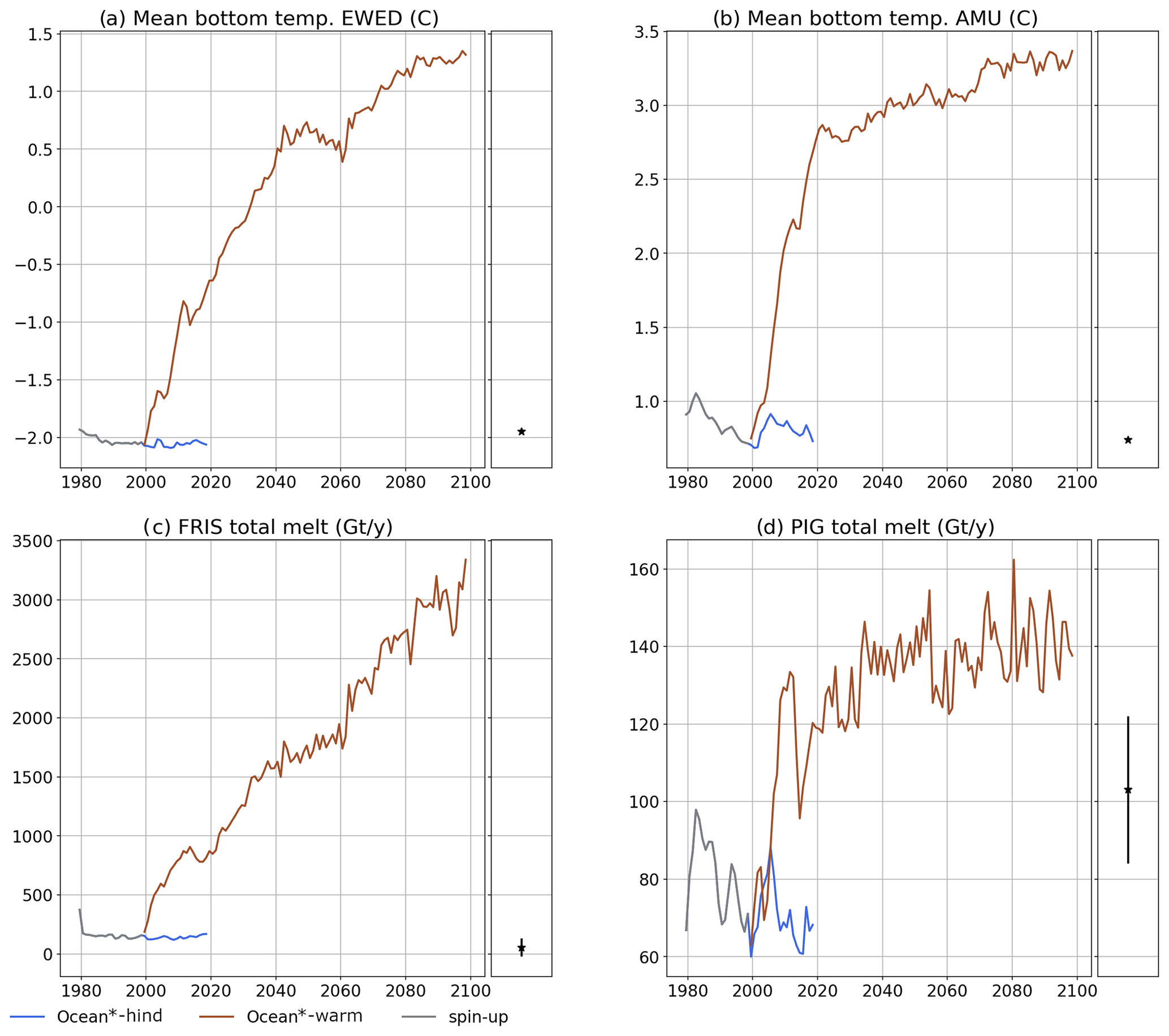
Figure 3 Example of results obtained by Mathiot and Jourdain (2023) in the OceanA-hind and OceanW-hind (blue) and OceanA-warm and OceanW-warm (brown) experiments. Top panels show the bottom temperature on the (a) east Weddell Sea (EWED; 78.63–76.90° S, 45.65–32.25° W) and (b) Amundsen Sea (AMU; 75.80–71.66° S, 109.64–102.23° W) continental shelf. Lower panels show total melt integrated beneath (c) Filchner–Ronne and (d) Pine Island ice shelves (FRIS and PIG, respectively). Black stars on the right are the observational estimates from the World Ocean Atlas 2018 (Locarnini et al., 2019) for the bottom temperature and from Paolo et al. (2023a) for the ice-shelf melt. Here the perturbation experiment starts in 2000, and the anomaly is added to the 2000–2018 atmospheric forcing, as well as to repeated cycles of the 1979–2018 forcing.

2.4 OceanA-ctrl and OceanW-ctrl experiments

Because of possible model drifts in the absence of a perturbation, in particular for global models, we need a control simulation that is similar to the perturbed experiments (i.e. Ocean^*-warm) but with zero anomaly in the forcing. All the sensitivity analyses will be undertaken with respect to this control simulation.

The OceanA-ctrl and OceanW-ctrl experiments represent extensions of the OceanA-hind and OceanW-hind experiments obtained by cycling the forcing used in the latter. In the case where only one cycle of present-day conditions is used in OceanA-warm and OceanW-warm experiments (i.e. n=0 in Fig. 2 and Table 1), no extension is required. In other cases, the extension will start immediately after OceanA-hind and OceanW-hind, as shown in Fig. 2. Note that as for the OceanA-warm and OceanW-warm experiments, the time variable will continue forward for the time cycles; e.g. it will indicate 2015–2050 in an extension over a second cycle of the 1979–2014 present-day period.

2.5 OceanA-Pgeom, OceanA-Fgeom, OceanW-Pgeom, and OceanW-Fgeom experiments

2.5.1 Aim

These experiments will be used to compare the basal melt response to an imposed change in the geometry of the Amundsen and Weddell seas ice-shelf cavities. Simulations are carried out with stand-alone ice-shelf–ocean models for two different ice-shelf cavity shapes: one present-day geometry (experiments with Ocean^*-Pgeom) and one hypothetical future geometry (experiments with Ocean^*-Fgeom). Further details about the geometries are provided below. The aim is to identify and compare the modelled feedbacks between changes in cavity geometry, ocean circulation, and basal melt rates for semi-realistic patterns of ice-shelf thinning and grounding-line retreat. Such feedbacks have previously been shown to be important for the evolution of the ice-shelf mass balance over interannual to decadal timescales (e.g. Holland et al., 2023; De Rydt and Naughten, 2024).

2.5.2 Type of models

The model requirements are identical to those for the Ocean^*-hind experiments. Models need to be able to implement the prescribed ice-shelf geometries.

2.5.3 Time window

Experiments with present-day and future cavity geometries both cover the same time window as Ocean^*-hind, following a spin-up period with the imposed ice-shelf geometry, as shown in Fig. 2. Present-day and future geometries each have their own spin-up.

2.5.4 Input/forcing

The forcing is the same as for Ocean^*-hind, i.e. the CAYA approach, except that a common bathymetry, as well as present-day (OceanA-Pgeom and OceanW-Pgeom) and future (OceanA-Fgeom and OceanW-Fgeom) ice-shelf draft, is imposed in the area from Dotson to Cosgrove (A) or in the region covered by the Filchner–Ronne Ice Shelf (W).

For the Ocean^*-Pgeom experiments, participants are asked to use the BedMachine Antarctica v3 dataset (Morlighem, 2022) for the bathymetry and present-day ice draft. For some groups, this geometry might be very similar to the geometry in their Ocean^*-hind experiments, for example, when an earlier version of the BedMachine dataset was used. For consistency, we ask participants to only provide results for the OceanA-Pgeom and OceanW-Pgeom experiments based on the exact BedMachine Antarctica v3 topography.

For the OceanA-Fgeom and OceanW-Fgeom experiments, participants are asked to use the same bathymetry from BedMachine Antarctica v3 but with a modified ice-shelf draft. The latter is provided as part of the MIPkit and is in the same format as BedMachine Antarctica v3. The original BedMachine v3 values were left unchanged outside of the Amundsen and Weddell sea regions, with a linear transition to the modified geometry over a 10 km halo. The future ice draft for the OceanA-Fgeom experiment was produced with the coupled ice–ocean model, Úa–MITgcm, starting from a present-day ice-sheet geometry and forced by constant shallow-thermocline conditions on the Amundsen continental shelf for 200 years (De Rydt and Naughten, 2024). The difference in ice thickness between the A-Pgeom and A-Fgeom geometries is shown in Fig. 4. For the OceanW-Fgeom experiment, the future ice draft is taken from an unpublished 300-year simulation with the coupled ice–ocean model Úa–MITgcm. The model configuration is identical to the abrupt-4xCO2 experiment described in (Naughten et al., 2021) but extended from 150 to 300 years based on a new time series of atmospheric and ocean boundary conditions from the UKESM1-0-LL CMIP6 ensemble. The difference in ice thickness between the W-Pgeom and W-Fgeom geometry is shown in Fig. 4. Global or circum-Antarctic models can run the experiments in a single simulation.

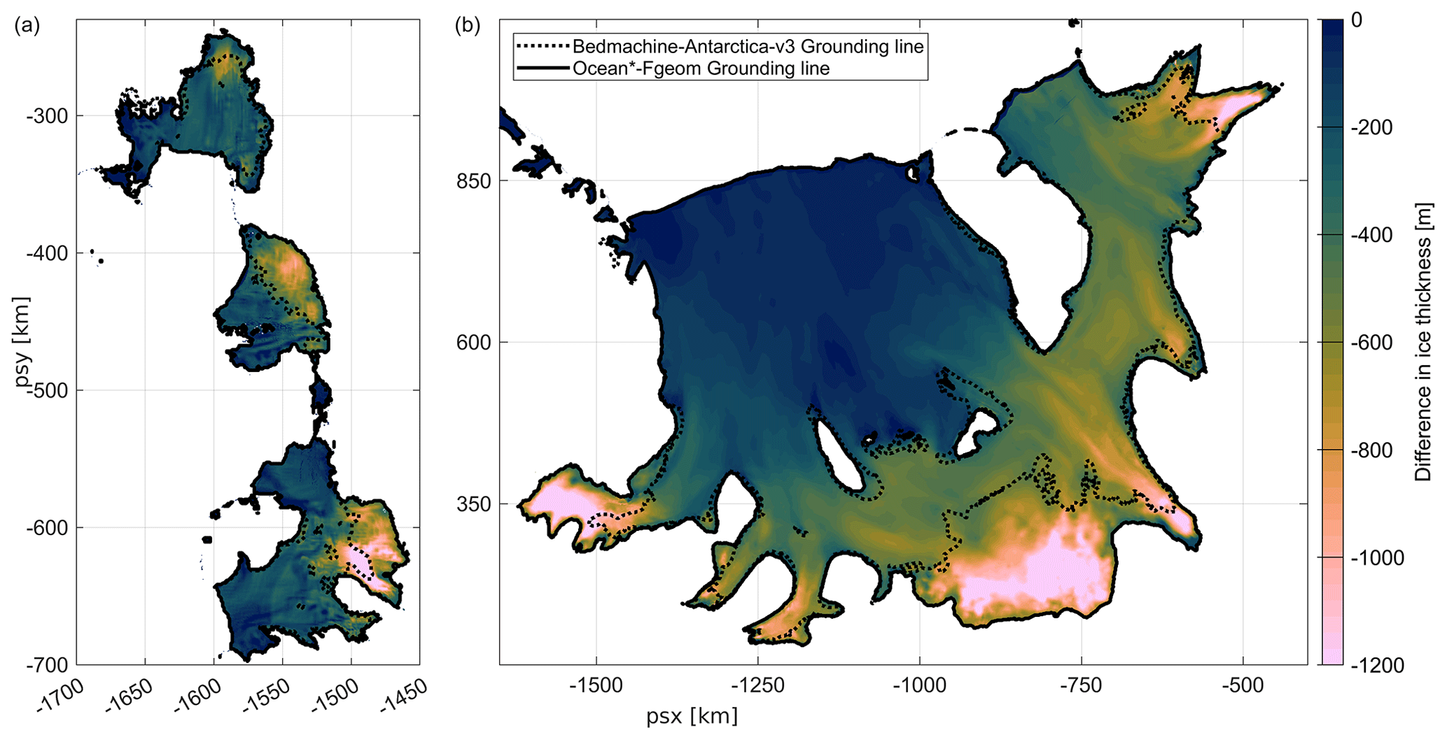
Figure 4 Difference in ice thickness between the Pgeom and Fgeom experiments for (a) the Amundsen Sea and (b) the Weddell Sea. The geometry for the Pgeom experiments is taken from BedMachine Antarctica v3, and the geometry for the Fgeom experiments is taken from Úa–MITgcm simulations, as described in the main text. The dotted and solid black lines correspond to the grounding lines for present-day (Pgeom) and future (Fgeom) geometries, respectively.

2.6 IceOceanA-hind and IceOceanW-hind experiments

2.6.1 Aim

The objectives of the IceOceanA-hind and IceOceanW-hind experiments are analogous to MISOMIP1 but with a broader focus on the model evaluation rather than the verification of initial coupling developments. We invite contributions from coupled ice-sheet–ocean models to assess their ability to hindcast observed changes in ice volume, ice dynamics, and grounding-line location, as well as ice-shelf melting and ocean changes. As with OceanA-hind and OceanW-hind, the MISOMIP2 protocol advocates a CAYA approach to these experiments.

The main focus of this exercise will be on the Amundsen Sea region, which has seen substantial changes over the 1990–2020 time period, with a strong negative mass balance and a significant acceleration in mass loss. The Weddell Sea sector has remained relatively unchanged and is assumed to be close to balance, but models need to be able to demonstrate this too, as capturing steady conditions can be challenging for some model set-ups (Comeau et al., 2022). Model outputs for these contrasting cases will be compared between different models and to available oceanographic and glaciological observations.

2.6.2 Type of models

The experiments should be performed by coupled ice-sheet–ocean models, i.e. models in which the ocean state evolves as a result of ice-shelf melt and the evolution of ice-shelf thickness and ice-sheet grounding lines. This includes the option of using coarse-resolution ocean models coupled to an ice-sheet model through a parameterization with no explicit representation of the ocean circulation in ice-shelf cavities. Instead, a basal melt parameterization can be forced by “far-field” ocean conditions and the calculated meltwater added as a freshwater (virtual salt) flux at the front of the closed cavities (e.g. Kreuzer et al., 2021). There are no geographical restrictions on the ocean domain in these experiments. We also note that such ocean set-ups should not contribute to the Ocean^*-hind, Ocean^*-Pgeom, and Ocean^*-Fgeom experiments, as they are targeting models with (thermo)dynamically interactive ice-shelf cavities.

The ocean model can be coupled to any type of ice-sheet/glacier model, from pan-Antarctic to smaller regional domains, ideally including the following drainage basins:

• for the Amundsen Sea at Pine Island, Thwaites, Smith, Pope, and Kohler glaciers and

• for the Weddell Sea at Evans, Carlson, Rutford, Institute, Möller, Foundation, Support Force, Recovery, Slessor, and Bailey ice streams.

Additional levels of complexity in the coupling procedure involving, e.g. the evolution of the ice-shelf calving front (Asay-Davis et al., 2016), the representation of iceberg drift (Smith et al., 2021), or subglacial freshwater discharge (Nakayama et al., 2021), are welcome but not required.

2.6.3 Time window

Models will ideally simulate ocean and ice dynamics over the past 3 decades (1990–2020). If this is not possible, simulations should start in the mid-2000 decade at the latest. We welcome outputs starting earlier, e.g. from 1979, for models able to represent this period. However, limited observations exist in the 1980s, so results from this time period will be almost exclusively used for model intercomparison.

2.6.4 Input/forcing

Participants are encouraged to follow the CAYA approach, in particular with respect to the surface and lateral boundary conditions, with the loose constraint that the initial ice-sheet state should be as representative as possible of the geometry and dynamics observed a few decades ago. This can be obtained from a formal inversion using observations, from a calibrated or selected spin-up phase, or from a combination of both. For example, for an initial configuration with nominal timestamp in the early 2000s, participants can use the BedMachine bathymetry, the ICESat-corrected ERS-1 digital elevation model (DEM) with a nominal timestamp of January 2004 (Bamber et al., 2009), and concurrent MeaSUREs surface velocity data (Mouginot et al., 2017b) to constrain their inversion. For an initial configuration in the mid-2000s to late 2000s, we recommend the use of recent topography products such as BedMachine Antarctica v3 (Morlighem, 2022) and one of many suitable ice velocity products.

2.7 IceOceanA-warm and IceOceanW-warm experiments

These experiments undergo the same ocean perturbation and are run for the same duration as the OceanA-warm and OceanW-warm experiments. The ice-sheet surface mass balance and other potential surface conditions (e.g. atmospheric temperature above the ice sheet) remain unchanged compared to IceOceanA-hind and IceOceanW-hind. The requested outputs are the same as IceOceanA-hind and IceOceanW-hind, with a continuous time variable over several cycles of the present-day period.

2.8 IceOceanA-ctrl and IceOceanW-ctrl experiments

This is an extension of IceOceanA-hind and IceOceanW-hind over several present-day cycles, and therefore with repeated conditions similar to the present, to be used as control for the IceOceanA-warm and IceOceanW-warm experiments.

3 MIPkit

For both the Amundsen and Weddell sectors, the initial version of the MIPkit consists of ocean and ice data that are formatted to be directly comparable to the model outputs (described in the next section), as well as the input files needed for coordinated perturbation experiments. In summary, the following points apply:

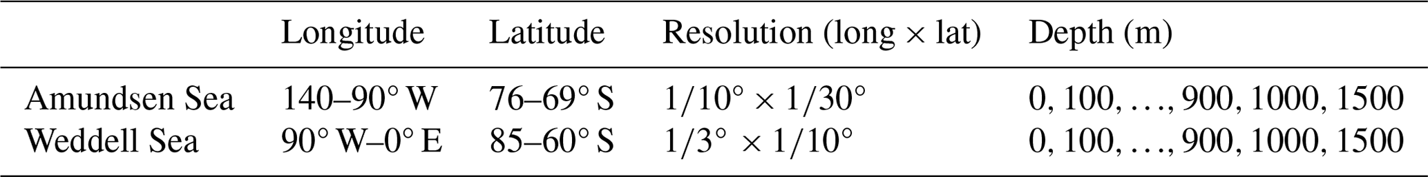
• Instantaneous ocean temperature (T) and salinity (S) are sampled on horizontal depth levels at 100, 200, 300, 400, 500, 600, 700, 800, 900, 1000, and 1500 m from available conductivity, temperature, and depth (CTD) values in the intercomparison domain. These observations will be used for the evaluation of large-scale hydrographic structures.

• Instantaneous ocean T and S values are taken from CTD values on a few chosen vertical sections at a higher vertical resolution, which will be used for a finer evaluation of the thermocline and pycnocline evolution across the continental shelf.

• Monthly mean T and S values are taken at a few mooring sites, providing a longer observational window (seasonal and interannual).

• Annual ice surface velocities and surface elevation changes from available Earth-observation products will be used for the evaluation of the present-day state of the ice sheet and its dynamical evolution over the observational period. We do not expect participants to use these data to initialize their models, but they can be a helpful tool to evaluate their set-ups.

• Perturbed atmospheric forcing (warm experiments) and ice-sheet perturbed geometry (A-Fgeom/W-Fgeom experiments) are used.

Importantly, the provided CTD measurements are representative of summer conditions, so model outputs will need to be considered in summer as well for evaluation.

We may evaluate the simulated ice-shelf basal melt rates based on several types of data, including the autonomous phase-sensitive radio-echo sounder (ApRES), which will be facilitated by the NECKLACE project (https://necklaceproject.com, last access: 17 September 2024); estimates from remote sensing and regional climate models (Rignot et al., 2013; Moholdt et al., 2014; Shean et al., 2019; Adusumilli et al., 2020; Paolo et al., 2023a); and estimates from CTD measurements (Dutrieux et al., 2014; Jacobs et al., 2011; Jenkins et al., 2018). However, ApRES tends to resolve finer spatial scales than those resolved in models, and other methods have large and somewhat unconstrained error bars over short to interannual timescales, so the use of these data in MISOMIP2 will be considered during the analysis of the MISOMIP2 contributions.

The different parts of the MIPkit are gathered in the MISOMIP2 community on Zenodo at https://zenodo.org/communities/misomip2 (last access: 17 September 2024).

3.1 MIPkit–A (Amundsen)

MIPkit–A contains both ice-sheet and ocean data. For the ice sheet, annual maps of ice surface velocity and surface elevation change are provided for the time periods 2000–2019 and 1992–2019, respectively. The datasets were compiled from available Earth-observation data and linearly interpolated onto the MISOMIP2 common grid (Table 4). For the surface velocities, a weighted average of the data from the MeaSUREs project (Rignot et al., 2014b; Mouginot et al., 2017a) and MeaSUREs ITS_LIVE project (Gardner et al., 2022) is provided, with weights corresponding to the inverse square error in the original datasets. For the surface elevation changes, a weighted average of the data from CPOM (Otosaka et al., 2023; Bevan et al., 2023) and MeaSUREs ITS_LIVE (Nilsson et al., 2023) for the grounded-ice and MeaSUREs ITS_LIVE data (Paolo et al., 2023a, b) for floating ice is provided. Both datasets include propagated errors and a mask indicating the original data sources for each grid point.

The ocean data consist of hydrographic properties along horizontal and vertical sections. The hydrographic properties provided on horizontal sections at 15 depths (every 100 m) come from the CTD measurements obtained during cruises of the following icebreaker research vessels (R/Vs): Nathaniel B. Palmer (United States Antarctic Program), James Clark Ross (British Antarctic Survey and Natural Environment Research Council), Araon (South Korea Polar Research Institute), Oden (Swedish Polar Research), and Polarstern (Alfred Wegener Institute, Germany). Here we have gathered data for the first months of 1994 (Jacobs, 1994), 2000 (Jacobs, 2000), 2007 (Jacobs, 2007), 2009 (Jacobs, 2009), 2010 (Swedish Polar Research Secretariat, 2010; Gohl, 2015), 2012 (Kim et al., 2012), 2014 (Heywood, 2014; Ha et al., 2014), 2016 (Kim et al., 2016), 2017 (Gohl, 2017), 2018 (Kim et al., 2018), 2019 (Larter et al., 2019), and 2020 (Wellner, 2020).

These data have been used in a number of scientific studies from the discovery of intrusions of warm deep water towards peripheral Antarctic ice shelves (Jacobs et al., 1996) to the description of the interannual variability in ocean properties on the continental shelf (e.g. Nakayama et al., 2013; Dutrieux et al., 2014; Heywood et al., 2016; Kim et al., 2016; Webber et al., 2017; Jacobs et al., 2011; Jenkins et al., 2018). In front of the Pine Island and Dotson ice shelves, the thermocline rose in the mid-2000s and remained high from 2006 to 2011, associated with an increased heat content over the continental shelf. The thermocline was back to a relatively deep position from 2012 to 2017 (Naughten et al., 2022).

The first vertical section for which we provide hydrographic data in the Amundsen Sea starts across the continental shelf break and follows the eastern Pine Island Trough southward until the Pine Island Ice Shelf. This section was monitored by the following cruises: N.B. Palmer in January 2009, Polarstern in March 2010, and Araon in February–March 2012 (Gohl, 2015; Dutrieux et al., 2014; Jacobs et al., 2011). The second vertical section starts across the continental shelf break and follows the Dotson–Getz Trough southward until the Dotson Ice Shelf. It was monitored by the aforementioned Araon expeditions in 2010–2011 and early 2012 (Kim et al., 2017).

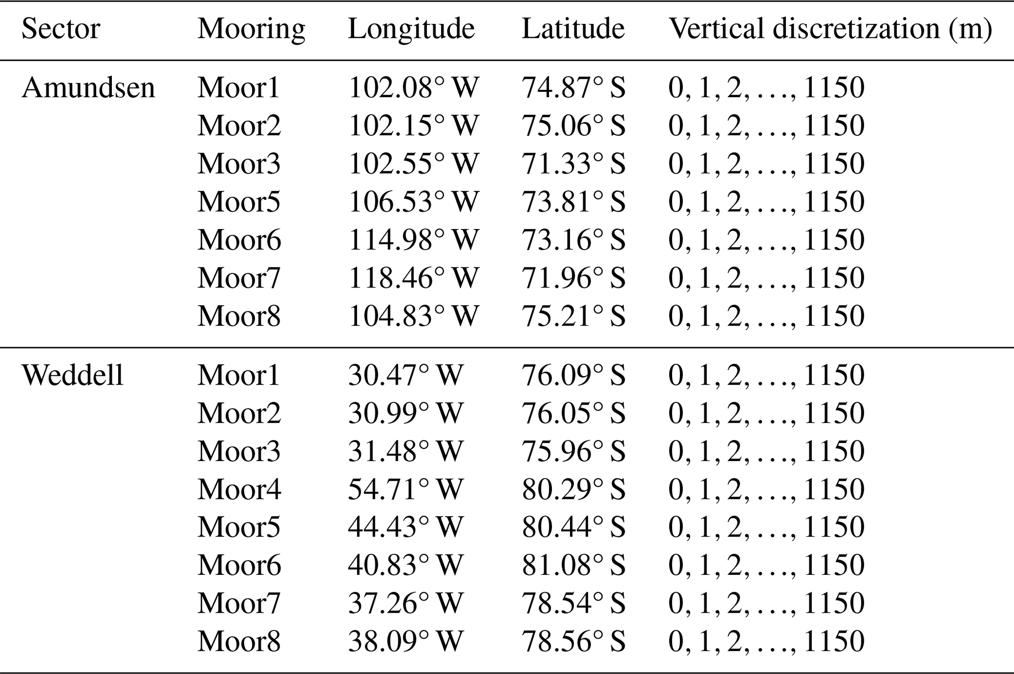
We will also conduct model–data comparisons for multi-year mooring observations (Table 3). The first mooring site is located near the northern part of the Pine Island Ice Shelf front (74.87° S, 102.07° W) and captures the thermocline variability from 2012 to 2018 (labelled “iSTAR-8” in the Natural Environment Research Council (NERC) iSTAR programme and “pig-n” in the NERC Ocean Forcing Ice Change programme). The second mooring site is located near the southern part of the Pine Island Ice Shelf front (75.05° S, 102.15° W) and was monitored between 2009 and 2016. Then, in 2019–2020, it was monitored through the following moorings: “BSR-5” (buoy-supported riser; Jacobs, 2009) and “iSTAR-9” (NERC iSTAR programme) and “pig-s” (NERC Ocean Forcing Ice Change programme). This second site experienced a strong deepening of the thermocline in 2012–2013 (Webber et al., 2017) and then a more moderate deepening in 2016. These two mooring sites are located only 20 km from each other, show distinct mean thermocline depth, and have more consistent variability (Joughin et al., 2021).

The third mooring observation (“trough-e” in the NERC Ocean Forcing Ice Change programme) used in MISOMIP2 is at the eastern Pine Island Trough (71.33° S, 102.55° W). The eastern trough is considered to be the entrance of modified Circumpolar Deep Water reaching the Pine Island Ice Shelf (Nakayama et al., 2013; Webber et al., 2017; Jacobs et al., 2011), but only 2 years of mooring observations were conducted from 2014–2015 due to sea-ice cover.

The fourth mooring site used in MISOMIP2 is at the western Pine Island Trough (71.56° S, 113.05° W). Several mooring observations were conducted within 2 km of each other, allowing us to observe thermocline variability from 2009 to 2016 with a 1-year gap in 2011 with the following moorings: “BSR-12” (Jacobs, 2009), “iSTAR-1” (NERC iSTAR programme), and “trough-w” (NERC Ocean Forcing Ice Change programme).

The fifth mooring observation (“mid-shelf” in the NERC Ocean Forcing Ice Change programme) used in MISOMIP2 is in the middle of the eastern Amundsen Sea in the submarine glacial trough connecting open water and the Pine Island and Thwaites ice shelves (73.81° S, 106.53° W). Two mooring observations were conducted within a few kilometres of each other, allowing us to observe the thermocline variability from 2012 to 2018 with the following moorings: “iSTAR-6” (NERC iSTAR programme) and mid-shelf (NERC Ocean Forcing Ice Change programme).

The sixth and seventh moorings used in MISOMIP2 are located in the Getz–Dotson Trough (71.16° S, 114.99° W and 71.96° S, 118.46° W). They were originally deployed under the names “BSR-7” and “BSR-14” (Jacobs, 2009), and further deployments were conducted by the Korea Polar Research Institute. These mooring observations have been used to study the inflow of warm-ocean heat towards the Getz and Dotson ice shelves (Kim et al., 2016, 2017, 2018).

The eighth mooring used in MISOMIP2 is located beneath the Thwaites Ice Shelf (75.21° S, 104.83° W) and was used to study the ice-shelf cavity environment in 2020–2021 (Davis et al., 2021, 2023).

3.2 MIPkit–W (Weddell)

Similar to MIPkit–A, the MIPkit–W contains both ice-sheet and ocean data. The ice-sheet data were obtained from the same data sources and using the same methods as described in Sect. 3.1 for MIPkit–A.

For the evaluation of the ocean-model performance in the Weddell Sea sector, we focus on the interaction between the far-field general circulation and the processes on the continental shelf and in the ice-shelf cavities.

The hydrographic properties provided on horizontal sections at 15 depths were derived from the CTD measurements obtained from late December to early March by the Alfred Wegener Institute (AWI), Bremerhaven, during Polarstern cruises ANT-XII/3 (Schröder, 2010), PS82 (Schröder and Wisotzki, 2014), PS96 (Schröder et al., 2016), and PS111 (Janout et al., 2019), which cover the years 1995, 2014, 2016, and 2018, respectively.

The first vertical section for which we provide hydrographic data goes from the tip of the Antarctic Peninsula to Kapp, Norway (12.33° E). It is known as WOCE SR04 and has been monitored since 1989. It captures the water masses that feed the continental shelf and those that have been modified by ice-shelf–ocean interaction, including newly formed bottom water. The surface water and the subsurface winter water influence the sea-ice formation and thus the production of the high-salinity shelf water (HSSW) that enters FRIS cavity. The intermediate Warm Deep Water (WDW), i.e. the Circumpolar Deep Water that upwelled in the Weddell Sea, is an important heat source that – modified to some degree – episodically enters the Filchner Trough and might reach the cavity (Ryan et al., 2020). The water masses below WDW, i.e. the Weddell Sea Deep Water (WSDW) and Weddell Sea Bottom Water (WSBW), are products of mixing between the HSSW and the Ice Shelf Water (ISW) formed in the depths of the FRIS cavity. The data provided were collected during Polarstern cruises in September–October 1989, November–December 1990, December 1992–January 1993, March–May 1996, April–May 1998 (Fahrbach and Rohardt, 1990, 1991, 1993, 1996, 1998), January–April 2005 (Rohardt, 2010), February–April 2008 (Fahrbach and Rohardt, 2008), December 2010–January 2011 (Rohardt et al., 2011), and December 2012–January 2013 (Rohardt, 2013), as well as December 2016–January 2017 and December 2018–February 2019 (Rohardt and Boebel, 2017, 2020).

The second vertical section is at ∼ 76° S and covers the eastern side of the Filchner Trough. It was surveyed during some of the aforementioned Polarstern cruises on 5–8 January 2014, 20–24 January 2016, and 4–23 February 2018. These sections show episodic signs of intruding modified WDW.

The third and fourth sections were obtained along the front of Ronne and Filchner ice shelves, respectively. The Filchner section was measured on 1–3 February 1977 (Foldvik et al., 1985) and 7–16 January 1981 (Hubold et al., 1982) from the Norwegian R/V Polarsirkel and then during several of the Polarstern cruises on the following dates: 25 January–4 March 1995, 15–17 January 2014, 15 January 2016 (only one vertical profile), and 14–23 February 2018. The Ronne section was measured on 25 January–24 February 1995, 14–15 January 2016, and 9–14 February 2018 as part of a continuation of the Filchner section measurements. These sections showed the properties and location of in- and outflow to/from the ice-shelf cavity and their variability.

Finally, three moorings placed along the 76° S vertical section give insight into the variability in the intrusions of modified WDW and five moorings underneath Filchner–Ronne Ice Shelf to access the intrusion of HSSW and production of ISW. The 76° S moorings are originally referred to as AWI252 (30.47° W), AWI253 (30.99° W), and AWI254 (31.48° W) and cover the period from January 2014 to February 2018 (Schröder et al., 2017a, b, c, 2019a, b, c). Temperature, salinity, and velocity data were obtained at two depths for AWI252 (335 and 421 m depth for a seafloor at 447 m) and AWI253 (349 and 434 m depth for a seafloor at 456 m), while a single depth is provided for AWI254 (553 m for a seafloor at 581 m). The moorings under the ice shelf were designed to collect data representative of the entire water column from the ice-shelf base to the seafloor at each location and capture interannual variability linked to large-scale atmospheric circulation (Hattermann et al., 2021). For our goals, we provide monthly means, but it is important to mention that the area is influenced by high-frequency variability.

3.3 MIPkit perturbations

This MIPkit contains all data needed to run the perturbation experiments, including the perturbations to add to the atmospheric forcing and possibly to the ocean lateral boundaries (A-warm and W-warm experiments), as well as the perturbed ice-shelf geometry (A-Fgeom, W-Fgeom). More details are provided in Sect. 2.

3.4 Living MIPkit

While an effort has been made to gather existing Earth-observation and in situ data for the ice sheet and ocean as part of the initial release of the MISOMIP2 protocol, we consider the MIPkit to be a living archive. We expect the MIPkit to be updated with new observational products reformatted for MISOMIP2 as necessary. The ongoing updates will be associated with version numbers on Zenodo. The MIPkit is nonetheless not intended to be a complete archive of all available data but rather a representative subset of observations that have been reformatted for easy comparison to the required model output.

4 Requested model outputs

Although we do not plan to upload the MISOMIP2 data onto the Earth System Grid Federation (ESGF) to keep some flexibility, we believe that a step toward more standardization than in MISOMIP1 will make our intercomparison more robust and reproducible and will facilitate potential future contributions of our community to CMIP and ISIMIP (Inter-Sectoral Impact Model Intercomparison Project).

For all the outputs described hereafter, we encourage participants to use the NetCDF 4 format with a simple precision for floats, a deflation level of 1, and chunking along the vertical and time dimensions set to 1, which should save space and facilitate the data processing.

4.1 Ocean outputs

Monthly mean outputs will be submitted on standard horizontal and vertical grids, namely a three-dimensional grid with few vertical levels used to plot horizontal slices, a few vertical sections to coincide with shipborne CTD sections (included in the MIPkit), and a few profiles at a single location for direct comparison to existing mooring data (included in the MIPkit). An overview of the sections and mooring profiles in the MIPkit, as well as the requested locations for model sections and profiles, is provided in Fig. 1. The common grids, list of requested variables, and recommended interpolation methods are provided below.

4.1.1 File-naming convention and common grids

The following three types of files will be provided by participants:

• Oce3d_<institute>_<model>_<abc>_<exp>_<period>.nc,

• OceSec<n>_<institute>_<model>_<abc>_<exp>_<period>.nc, and

• OceMoor<n>_<institute>_<model>_<abc>_<exp>_<period>.nc,

where <n> is the section or mooring number; <model> is the model name, possibly including a version number; <institute> is the name of the institute(s) that produced the simulation (use “-” rather than “_” for multiple entities); <abc> is a single letter used to distinguish multiple set-ups produced by a given institute (e.g. variation in model parameters, resolution, initial states or boundary conditions); <exp> is the MISOMIP2 experiment name (e.g. OceanA-hind, OceanW-hind, and IceOceanA-hind); and <period> indicates the starting year and month and the final year and month (e.g. 197901-202012). The simulations can be split into as many time segments as desired. Note that modelling groups that provide regional simulations for both the Amundsen and Weddell sectors should use the same letter in <abc> only if the modelling set-up is exactly the same (apart from the domain location).

• The Oce3d files cover monthly mean fields on the three-dimensional common grids described in Table 2 and shown in Fig. 1 and contain all the ocean variables discussed hereafter.

• The OceSec files contain potential temperature and salinity along six observed vertical sections, four in the Weddell Sea and two in the Amundsen Sea, as described in Sect. 3. The (lon,lat,lev) locations of the requested data are provided in preproc/def_grids.py on https://github.com/misomip/misomip2 (last access: 17 September 2024) or as .csv files in the MIPkit–A and MIPkit–W datasets (https://zenodo.org/communities/misomip2, last access: 17 September 2024). Vertical coordinates are uniformly spaced at 10 m intervals between 0 m and 1150 m, except for the SR04 section between Kapp, Norway, and the tip of the Antarctic Peninsula, for which data should be provided at 10 m depth intervals between 0 m and 5000 m.

• The OceMoor files contain vertical profiles of potential temperature and salinity at 16 locations (listed in Table 3). At each location, the data are requested at 1 m vertical resolution between 0 m and 1150 m. The (lon,lat,lev) coordinates in Table 3 are also available in preproc/def_grids.py on https://github.com/misomip/misomip2 or as .csv files in the MIPkit–A and MIPkit–W datasets.

Table 2 Common grid parameters used for Oce3d files.

Table 3 Location of mooring data.

4.1.2 Dimensions, variables, and metadata

The requested output format follows the NetCDF Climate and Forecast (CF) Metadata Convention. The dimensions of the common ocean grids are (lon,lat,lev,time,bnds), and their corresponding variables and attributes are defined in the Appendix (Table A1).

The requested ocean variables are listed in Table A1. They are largely based on the CMIP6 data request and on the OMIP variables described in the appendices of Griffies et al. (2016), with additional variables introduced here to describe ice-shelf cavities and ice-shelf–ocean interactions, as well as a few new variables that are the sum of existing variables (underlined variables in Table A1). Note that for the perturbation experiments (Ocean^*-warm, Ocean^*-ctrl, IceOcean^*-warm, and IceOcean^*-ctrl), the time variable will continue forward over the time cycles; e.g. it will indicate 2001–2040 for two consecutive cycles forced by 2001–2020 boundary conditions.

Although several models have transitioned to the TEOS-10 seawater thermodynamics, which is formulated for a better representation of heat conservation and of the chemical compositions of seawater (IOC et al., 2010), many model formulations are still based on pre-TEOS-10 thermodynamics. For simplicity, we make the choice to stick to this formulation for MISOMIP2, although we believe that future intercomparisons would benefit from transitioning towards TEOS-10. Models that archived TEOS-10 quantities may use the Gibbs-SeaWater Oceanographic Toolbox to convert to pre-TEOS-10 quantities.

All time-dependent ocean variables are monthly means (over full calendar months). All of these variables have a fill value (_FillValue) set to 9.969209968386869e36 (standard missing value for floats in NetCDF); this value is attributed to any part of the MISOMIP2 domain that is not covered by the original domain (no extrapolation) and to cell fractions lower than 1 % (e.g. all the variables interpolated from ice-shelf cells are set to the fill value if the interpolated ice-shelf fraction is lower than 1 %). Note that according to this framework, some cells with a partial ice-shelf fraction have both a non-zero ice-shelf draft and non-zero sea surface fraction with corresponding surface temperature, salinity, etc.

We recommend that participants add a warning attribute for any variable that was recalculated offline based on specific assumptions, interpolated in an atypical way, or where its interpretation might otherwise require caveats.

We ask all contributors to indicate the main aspects of their modelling set-up as global attributes in the NetCDF files. This is an important part of the output that will facilitate the automatic display, analysis, and clustering of multi-model outputs. The requested global attributes for ocean outputs are listed in Table A2.

4.1.3 Interpolation methods

Because of the imposed regridding to the common grid, it is essential to clarify the interpolation method.

Conservative interpolation of coarse-resolution model output onto a fine grid imprints the coarse grid meshes (e.g. big rectangles) on the fine grid. When averaging multiple models, this may hide dynamical structures such as gyres and horizontal gradients. We therefore do not recommend using conservative interpolation for model grids of similar or coarser resolution than the MISOMIP2 standard grids. Instead, we recommend linear interpolation in the (lon×cos 〈lat〉,lat) space for all variables, where 〈lat〉 is the mean latitude over the MISOMIP domain. This is preferred to an interpolation in the (long, lat) space to have a more isotropic interpolation. As there is a variety of grid structures and projections, we recommend the linear triangular interpolation which may be suitable for all models. It consists of triangulating the input data and performing a linear interpolation in the barycentric coordinate system. For target points falling out of the convex zone, no triangular interpolation is possible, and a nearest-neighbour interpolation is recommended to fill these points. Bi-linear interpolation can also be performed for models on structured long–lat grids, and other similar linear methods are also accepted (e.g. ESMF_RegridWeightGen from the Earth System Modeling Framework (ESMF) library). For model grids of a significantly higher resolution than the standard MISOMIP2 grid, conservative interpolation or average-based grid coarsening prior to linear interpolation is a reasonable option.

For the model intercomparison, it is essential that interpolations consider whether a given variable is defined over the entire cell or only over a fraction of it. This is indicated through the cell_methods attribute in Table A1:

• area: mean indicates interpolation from all neighbour cells;

• area: mean where sea ice indicates interpolation from neighbour cells weighted by their sea-ice fraction;

• area: mean where ice shelf indicates interpolation from neighbour cells weighted by their ice-shelf fraction;

• area: mean over bottom ocean cells indicates interpolation from neighbour bottom-ocean cells;

• area: mean where ocean surface indicates interpolation from neighbour cells with ocean or sea-ice at the surface (ice shelves excluded);

• area: mean where 3d ocean indicates interpolation from neighbour cells with ocean at any depth (i.e. including ice-shelf cavities); and

• volume: mean where ocean indicates 3D interpolation from neighbour-ocean cells.

The recommended vertical interpolation method is a simple one-dimensional linear interpolation in depth coordinates. Non-Z-coordinate models therefore need to convert their outputs to Z coordinates prior to interpolation to the MISOMIP2 grids. Several vertical coordinate systems may depend on sea-surface height, which makes vertical levels fluctuate by a few metres at most. In MISOMIP2, we tolerate that this is not accounted for in the vertical interpolation as it can facilitate computations without altering the intercomparison to a significant extent. The interpolated value should cover the entire model wet cells, and uniform values can be used beyond the centre of the uppermost and lowermost cells.

4.2 Ice outputs

In addition to the aforementioned ocean outputs, all participants will provide yearly snapshots or means for a range of ice-sheet variables, including ice thickness, ice velocities, and the grounding-line location, on a predefined horizontal grid. The common grids, a list of requested variables (largely based on ISMIP6 requested variables; see Nowicki et al., 2016), and recommended interpolation methods are listed here.

File-naming convention and common grids

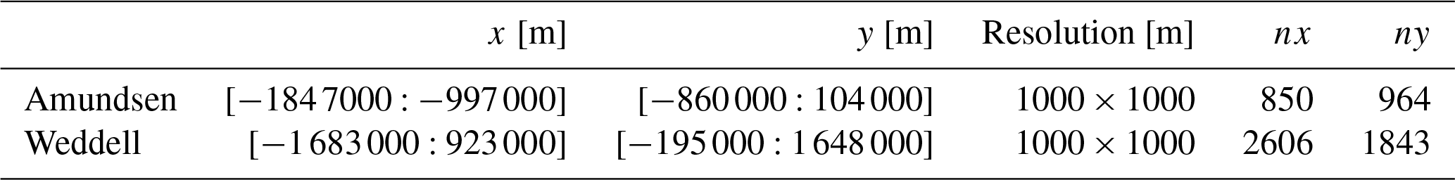
In MISOMIP2, we only request 2D ice-sheet variables provided as snapshots or yearly averages at the end of each year. Variables should be vertically averaged and interpolated onto cell centres of a regular horizontal grid with a uniform horizontal resolution of 1 km. The characteristics of the common grids for the Amundsen Sea and Weddell Sea domains are provided in Table 4 and shown in Fig. 1.

Table 4 Boundaries, resolution, and number of points of the standard ice grids. Coordinates use the EPSG:3031 Antarctic Polar Stereographic projection with a standard parallel −71° S and a central meridian 0° W.

Only one type of file will be provided by participants for ice outputs:

• Ice_<model>_<institute>_<abc>_<exp>_<period>.nc,

where <model>, <institute>, <abc>, <exp>, and <period> have been defined in the previous subsection.

Dimensions, variables, and metadata

The requested output format follows the NetCDF Climate and Forecast (CF) Metadata Convention. The dimensions of the common ice-sheet grids are (x,y,time,bnds), and their corresponding variables and attributes are defined in Table A3.

The requested ice variables are listed in Table A3. They are largely based on the CMIP6 data request and on the ISMIP6 variables described in Nowicki et al. (2016).

Interpolation methods

In contrast to ISMIP6, the primary aim of MISOMIP2 is to analyse dynamical patterns across a large range of model resolutions rather than to accurately quantify the evolution of the ice-sheet mass. Therefore, we do not request conservative interpolation. In the case of participating ice-sheet model grids that are much coarser than the 1 km common grid, linear interpolation methods (see examples in Sect. 4.1) should be preferred over conservative and nearest-neighbour interpolations to avoid misleading strong gradients on the common grid.

For the intercomparison between models, it is essential that interpolations consider whether a given variable is defined over the entire cell or only over a fraction of the cell. This is indicated through the cell_methods attribute in Table A3:

• area: mean indicates interpolation from all neighbouring cells, including nunataks, ocean, and ice sheet;

• area: mean where land ice indicates interpolation from neighbouring cells weighted by their land–ice fraction (grounded or floating);

• area: mean where ice shelf indicates interpolation from neighbouring cells weighted by their ice-shelf fraction; and

• area: mean where grounded ice indicates interpolation from neighbouring cells weighted by their grounded-ice fraction.

As in ISMIP6, we require snapshots for the state variables and yearly averages for the flux and tendency variables. This is indicated in Table A3 through the cell_methods attribute, which contains either time: instantaneous or time: yearly mean.

We ask all contributors to indicate the main aspects of their modelling set-up as global attributes in the NetCDF files to facilitate the automatic display, analysis, and clustering of multi-model outputs. The global attributes of the ice output file are listed in Table A4.

5 Conclusions and outlook

We have described the design of several interrelated ocean and coupled ice-sheet–ocean experiments for two targeted regions of Antarctica, collectively referred to as the Marine Ice Sheet–Ocean Model Intercomparison Project – phase 2 (MISOMIP2). A series of ocean-only and coupled ice-sheet–ocean experiments were designed to test the model fidelity and model sensitivity to a large prescribed anomaly in climate forcing. We expect that results from each part (ocean-only and coupled ocean–ice) will be published separately with all contributors as co-authors, following the tradition of earlier MIPs. We have tested the feasibility of all stand-alone ocean and ice-sheet–ocean experiments using several ocean and ice-sheet–ocean configurations, and we are confident that they can be run by other participants who use different model architectures and climatic forcing datasets. Future community activities will be determined based on the outcomes of the MISOMIP2 experiments. These potentially include, but are not limited to, experiments with a higher degree of similarity in climate forcing between contributing models, parameter and numerical choices, and forward simulations at multi-decadal to century timescales under a range of prescribed climate-change scenarios, aimed at coordinating with ongoing ISIMIP and CMIP efforts.

Appendix A

Griffies et al., 2016Griffies et al. (2016)(see Appendix H7 of Griffies et al., 2016)Griffies et al. (2016)Griffies et al. (2016)Griffies et al. (2016)Griffies et al. (2016)

Table A1 Requested ocean variable names (in bold) and their dimensions (in brackets) are listed in the first column, their corresponding attribute names and attribute values in the second and third column, respectively. Variables that are modified or newly introduced in this article are underlined. For time-dependent variables, monthly mean outputs are requested.

Table A2 Global attributes requested for the ocean outputs.

Table A3 Requested ice-sheet variable names (in bold) and their dimensions (in brackets) are listed in the first column, their corresponding attribute names and attribute values in the second and third column, respectively. Variables that are modified or newly introduced in this article are underlined.

Table A4 Global attributes requested for the ice outputs.