Development of a total variation diminishing (TVD) sea ice transport scheme and its application in an ocean (SCHISM v5.11) and sea ice (Icepack v1.3.4) coupled model on unstructured grids

As the demand for increased resolution and complexity in unstructured sea ice models is growing, higher demands are also placed on the sea ice transport scheme. In this study, we couple the Semi-implicit Cross-scale Hydro-science Integrated System Model (SCHISM, v5.11) with Icepack (v1.3.4), the column physics package of the Los Alamos sea ice model (CICE); a key step is to implement a total variation diminishing (TVD) transport scheme for the multi-class sea ice module in the coupled model. Compared with the second-order upwind scheme and the finite-element flux-corrected transport (FEM-FCT) scheme, the TVD transport scheme is overall superior when evaluated based on conservation, accuracy, efficiency (even with very high resolution), and strict monotonicity. Although it is slightly weaker than FEM-FCT in terms of accuracy alone, the TVD scheme still outperforms the other two schemes in comprehensive performance. The new coupled model outperforms the existing single-class ice model of SCHISM in the case of Lake Superior. For the Arctic Ocean case, it successfully reproduces the long-term changes in the sea ice extent, sea ice boundary, concentration observations from satellites, and thickness from in situ measurement.

1 Introduction

The dramatic decrease in the Arctic sea ice in recent decades attributable to global warming has a major impact on local and global climate (IPCC, 2019). In order to understand the changes in the physical and biogeochemical processes occurring in the Arctic Ocean, numerical models have become an important tool and they have been significantly improved in the past few decades. The sea ice, as a highly complex material (Hunke et al., 2020), has received special attention. Consequently, sea ice models have evolved, offering better representation of the sophisticated physical processes. At present, an advanced sea ice model, the Los Alamos sea ice model (CICE; Hunke et al., 2015), including the stand-alone column physics package Icepack (Hunke et al., 2020), has incorporated multi-class thermodynamics, such as the Bitz and Lipscomb (1999; BL99) thermodynamics formulation for constant salinity profiles, the mushy layer thermodynamics formulation for evolving salinity (Turner et al., 2013), and the sea ice ridging processes (Lipscomb et al., 2007). Many structured-grid models have been coupled with Icepack or CICE directly or via couplers, e.g., the Community Earth System Model (CESM; Hurrell et al., 2013) and the HYbrid Coordinate Ocean Model (HYCOM); others have partially incorporated and adapted CICE subroutines in their own ice module, e.g., the Sea Ice modelling Integrated Initiative (SI³) of the Nucleus for European Modelling of the Ocean (NEMO; NEMO can also couple with CICE or the Louvain-La-Neuve sea ice model, LIM3; Madec et al., 2022) and the Thermodynamic Sea Ice Package (THSICE) of the Massachusetts Institute of Technology General Circulation Model (MITgcm; Adcroft et al., 2023). For unstructured-grid (UG) models, Gao et al. (2011) have incorporated Unstructured-Grid CICE (UG-CICE) into the unstructured-grid Finite Volume Community Ocean Model (FVCOM; Chen et al., 2012). Some other unstructured-grid models have incorporated Icepack directly, e.g., the Finite-volumE Sea ice-Ocean Model version 2 (FESOM2; Zampieri et al., 2021) and the Model for Prediction Across Scales (MPAS-Seaice; Turner et al., 2022). UG-CICE and FESOM2 utilize triangular mesh grids, whereas MPAS-Seaice employs a Voronoi dual graph. UG-CICE is based on a finite-volume formulation, and the sea ice component allows for five ice categories, four layers of ice and one layer of snow. The remaining models permit user specification of the number of ice categories. UG-CICE can produce good results on the seasonal variability of the sea ice in the Arctic Ocean (Gao et al., 2011). FESOM2, having implemented Icepack comprehensively, demonstrates that additional complexity in model formulations can enhance simulation accuracy (Zampieri et al., 2021). MPAS-Seaice can be viewed as the unstructured version of CICE and thus shares sophisticated thermodynamics and biogeochemistry with CICE, including BL99 and the mushy layer, and is the current sea ice component of the Energy Exascale Earth System Model (E3SM; Turner et al., 2022). A summary of these sea ice models is given in Table 1.

Table 1 Comparison of several sea ice models.

SCHISM is a derivative product built from the original Semi-implicit Eulerian–Lagrangian Finite Element model (SELFE, v3.1dc; Zhang and Baptista, 2008) with multiple enhancements, including seamless cross-scale capability from creek to ocean and the mass-conservative, monotone, higher-order transport solver TVD² (implicit TVD in the vertical and explicit TVD in the horizontal; Y. J. Zhang et al., 2016). SCHISM has been applied to study the Great Lakes ice formation process and obtained reasonable results in very high resolution (Zhang et al., 2023) using a single-class ice and snow module borrowed from FESOM (Danilov et al., 2015). The employed thermodynamic approach utilizes a zero-layer thermodynamic module (Parkinson and Washington, 1979), with constant dry and melting albedos of ice and snow. In the simulation of the Great Lakes ice formation process, both SCHISM and the single-class ice model allow multi-scale physics at variable resolution, but the rate of melting within the model is more rapid than what has been observed (Zhang et al., 2023). In order to improve the simulation capability of ice, the implementation of the multi-class sea ice module, Icepack, is required.

When Icepack is coupled with another model, the latter must implement its own transport solver for ice. Hunke et al. (2010) suggested that the solver should be accurate, stable, conservative, strictly monotonic, and efficient. In the sea ice model, monotonicity ensures that the values of new tracers, such as ice thickness and enthalpy (but not ice concentration), do not exceed the local extrema, specifically the maximum or minimum values in their vicinity under pure advection (Lipscomb and Hunke, 2004), even when the ice concentration exceeds 1 and results in ridging, which has been described in Icepack. The methodology for sea ice transport has undergone extensive study over the years, resulting in the proposal of various schemes. Lipscomb and Hunke (2004) implemented the upwind and incremental remapping schemes in CICE, both of which are still available in the latest version. Although the upwind scheme is the simplest method for transport, its first-order accuracy results in excessive diffusion. The incremental remapping scheme is a second-order accurate scheme and has great performance in structured-grid models and MPAS-Seaice, but it requires an excessively small time step to avoid cross-trajectories when the velocity field is divergent (Lipscomb and Hunke, 2004) or for highly distorted UGs (Turner et al., 2022). MITgcm provides a variety of tracer advection solvers, with a recommendation for flux-limited schemes in order to prevent unphysical outcomes (Adcroft et al., 2023). NEMO uses either the Prather scheme or the ULTIMATE-MACHO scheme with the SI³ ice model (Madec et al., 2022), both of which require some functions to limit the tracer concentrations from exceeding the largest values of all adjacent nodes.

In the case of triangular UGs, the transport scheme utilized in UG-CICE is the second-order upstream scheme, which considers the gradient of sea ice tracers (Gao et al., 2011). This scheme is consistent with the tracer transport in FVCOM (Chen et al., 2012). The transport scheme of FESOM2 is the FEM-FCT (Löhner et al., 1987), which is based on the finite-element description (Danilov et al., 2015). It is also a conservative and second-order scheme (Budgell et al., 2007), but its cost linearly increases with the number of variables, and more importantly, strict monotonicity comes with a higher cost (Löhner et al., 1987). It is imperative to underscore that the requirement for strict monotonicity is designed to prevent unphysical values that can crash the model. Therefore, Zhang et al. (2023) used the modified FEM-FCT scheme by zeroing out certain higher-order contributions in their study for the single-class ice module with very high resolution.

This paper presents SCHISM–Icepack, an unstructured ice–ocean coupled model that updates SCHISM for Icepack. The coupled model utilizes the TVD transport scheme, which has been implemented in SCHISM for ocean tracers (Y. J. Zhang et al., 2016), to achieve an efficient, strictly monotone, second-order accurate scheme for ice tracers on generic unstructured grids (even with locally very high resolution). Section 2 introduces components of SCHISM–Icepack and describes how the TVD transport scheme is implemented for the ice model. In Sect. 3, we compare some ideal test results from the new TVD scheme with two other second-order accurate methods (the second-order upwind scheme and FEM-FCT). The efficiency of the TVD scheme is also compared with the upwind scheme when applied to a high-resolution mesh. Additionally, the results of the new coupled model are compared with those of the existing single-class ice model of SCHISM. The new coupled model is validated with a simulation of the Arctic Ocean sea ice using realistic atmosphere forcing. Section 4 summarizes the major findings of this work.

2 Method

2.1 Icepack implemented in SCHISM

SCHISM–Icepack is coupled by Icepack v1.3.4 (Hunke et al., 2023) and SCHISM v5.11. Besides the zero-layer thermodynamics, two more sophisticated thermodynamic formulations, BL99 and the mushy layer, are also implemented. At the sub-grid scale, thin ice and thick ice coexist, and therefore an ice thickness distribution (ITD; Lipscomb, 2001; Bitz et al., 2001) has been implemented in order to describe the unresolved spatial heterogeneity of the thickness field. The ITD offers a prognostic statistical description of the sea ice thickness, which it divides into multiple categories, along with the ice area fraction corresponding to each category – a more detailed approach than the singular fraction used in the previous implementation. More tracers and more ice processes are added in this coupled model by Icepack, including multiple melt pond parameterizations (Hunke et al., 2013) and a mechanical redistribution parameterization (Lipscomb et al., 2007) that responds to sea ice convergence by piling up thin sea ice and therefore mimicking ridging and rafting events. The interaction between the shortwave radiation and the sea ice in Icepack is addressed using two formulations: the Community Climate System Model (CCSM3) formulation, which relates the surface albedo to the surface sea ice temperature, and the delta–Eddington formulation (Briegleb et al., 2007), which relates the albedo to inherent optical properties of sea ice and snow. The dynamic solver is not included in Icepack and is based on two approaches: (1) the classic elastic–viscous–plastic method (EVP; Hunke and Dukowicz, 1997) and (2) the modified elastic–viscous–plastic method (mEVP; Kimmritz et al., 2015). Both methods are inherited from the previous single-class ice and snow formulation (Zhang et al., 2023). It is important to note the difference in grid definition between the ice module and the hydrodynamic module. The ice module uses the Arakawa-A grid, and all tracers and velocities are defined at nodes. But the hydrodynamic module uses the Arakawa-CD grid, with the velocities defined at the side centers and tracers at the prism center. The decision to employ an analog of the Arakawa-A grid in the rheology part, adapted from FESIM, was primarily based on its computational efficiency and success in sea ice simulation (Danilov et al., 2015). All ice-related subroutines are called at each time step in the ocean model by SCHISM's hydrodynamic core. The ice module exports to SCHISM variables needed for coupling such as the shortwave radiation, the ice–ocean heat flux, the freshwater flux, and finally the sea ice pressure and ice–ocean stress for all ice-covered nodes, in proportion to the sea ice area fraction. Over open ocean these variables are calculated directly by SCHISM. All variables required by Icepack can be obtained from either SCHISM or a separate input file. And the coupling between the ice module and the hydrodynamic module remains unaffected by the differences in the variable definition, as all forcing variables are located at nodes in the hydrodynamic module.

2.2 Schemes for sea ice transport

The basic transport equation of sea ice area or fraction a_n for each sea ice category is (Thorndike et al., 1975)

$$\begin{array}{}\text{(1)}& {\displaystyle \frac{\partial a_n}{\partial t}}+{\displaystyle \frac{\partial u{a}_n}{\partial x}}+{\displaystyle \frac{\partial v{a}_n}{\partial y}}+{\displaystyle \frac{\partial }{\partial h}}\left(a_{n}f\right)=\mathit{\psi },\end{array}$$

where u and v are the ice velocities of the x and y components, respectively, and h is the ice thickness. The last term on the left side is thermodynamic change, where f is the rate of ice melting or growing, and the right-side term ψ is mechanical redistribution like the ridging process. We solve this equation using a fractional step method: first solve a pure advection equation (i.e., by setting the thermodynamic term and mechanical redistribution term to 0), followed by a correction step that includes the remaining terms. The main challenge occurs in the first step, where we must solve a pure advection equation for one category of sea ice fraction a_n:

$$\begin{array}{}\text{(2)}& {\displaystyle \frac{\partial a_n}{\partial t}}+{\displaystyle \frac{\partial u{a}_n}{\partial x}}+{\displaystyle \frac{\partial v{a}_n}{\partial y}}=\mathrm{0}.\end{array}$$

Note that the ice velocity field can be divergent or convergent, which can produce new local maxima and minima for a_n. However, a strictly monotone scheme is still desirable in order to separate the numerical dispersion from the physical convergence, especially for tracers like ice enthalpy and salinity.

We apply a finite-volume algorithm to discretize Eq. (2). The sea ice module inside SCHISM employs an Arakawa-A grid, with the sea ice velocity, ice concentration, and other tracers located at the node (blue circles in Fig. 1). The control volume is defined as the polygon enclosed by the lines composed of centroids and edge centers (red circles in Fig. 1). So, in the subsequent time step, after Δt, the new ice fraction is

$$\begin{array}{}\text{(3)}& a_n^{t+\mathrm{1}}=a_n^t+{\displaystyle \frac{\mathrm{\Delta }t\sum _{i\in S}{Q}_i{\mathit{\varphi }}_i}{{\mathrm{\Omega }}_S}},\end{array}$$

where Ω_S is the total area of the control volume, S is its boundary, and Q_i is the flux across the edge i of the control volume. Most of these variables can be obtained easily in the model, so we only focus on finding a method to approximate the edge value, ϕ_i (this symbol always represents ice concentration hereafter).

The simplest method is the first-order upwind scheme (assuming, without loss of generality, the velocity direction is as depicted in Fig. 1):

$$\begin{array}{}\text{(4)}& {\mathit{\varphi }}_i={\mathit{\varphi }}_{\mathrm{C}}.\end{array}$$

The TVD corrects the upwind values as

$$\begin{array}{}\text{(5)}& {\mathit{\varphi }}_i={\mathit{\varphi }}_{\mathrm{C}}+{\displaystyle \frac{{\mathit{\psi }}_i}{\mathrm{2}}}\left({\mathit{\varphi }}_{\mathrm{D}}-{\mathit{\varphi }}_{\mathrm{C}}\right),\end{array}$$

where ϕ_C and ϕ_D are the values at the upwind and the downwind nodes, respectively, for one edge of the control volume (Fig. 1a). And the last term on right side is the anti-diffusion correction. In this part, ψ_i is a function of the upwind ratio, r_i, for which we select the van Leer limiter (van Leer, 1979),

$$\begin{array}{}\text{(6)}& {\displaystyle }{\mathit{\psi }}_i={\displaystyle \frac{r_i+\left|r_i\right|}{\mathrm{1}+\left|r_i\right|}},\text{(7)}& {\displaystyle }{r}_i={\displaystyle \frac{{\mathit{\varphi }}_{\mathrm{C}}-{\mathit{\varphi }}_{\mathrm{U}\ast }}{{\mathit{\varphi }}_{\mathrm{D}}-{\mathit{\varphi }}_{\mathrm{C}}}}.\end{array}$$

If r_i<0, it means ϕ_C is a local extreme, and ϕ_i in Eq. (5) will revert to upwind. If r_i>0, there is no local extreme, and ${\mathit{\psi }}_i\in [\mathrm{0},\mathrm{2})$, so ϕ_i is a weighted average of ϕ_C and ϕ_D in Eq. (5). And here, ϕ_U∗ is defined as the upwind node of the upwind node (i.e., “up-upwind”) and can be accessed easily in a structured grid or a uniform unstructured grid (Fig. 1a). But for generic unstructured grids, how to approximate ϕ_U∗ is a key issue for the TVD scheme. There are several possible choices for ϕ_U∗, and after some comparisons we choose the method proposed by Darwish and Moukalled (2003). This method includes the gradient of the central node ∇ϕ_C,

$$\begin{array}{}\text{(8)}& {\mathit{\varphi }}_{\mathrm{U}\ast }={\mathit{\varphi }}_{\mathrm{D}}+{\mathit{R}}_{\mathrm{DU}}\cdot \left(\mathrm{\nabla }{\mathit{\varphi }}_{\mathrm{C}}\right)={\mathit{\varphi }}_{\mathrm{D}}-\mathrm{2}{\mathit{R}}_{\mathrm{CD}}\cdot \left(\mathrm{\nabla }{\mathit{\varphi }}_{\mathrm{C}}\right),\end{array}$$

where R_DU is the vector from the downwind node to the up-upwind node, and R_CD is the vector from the upwind to downwind nodes.

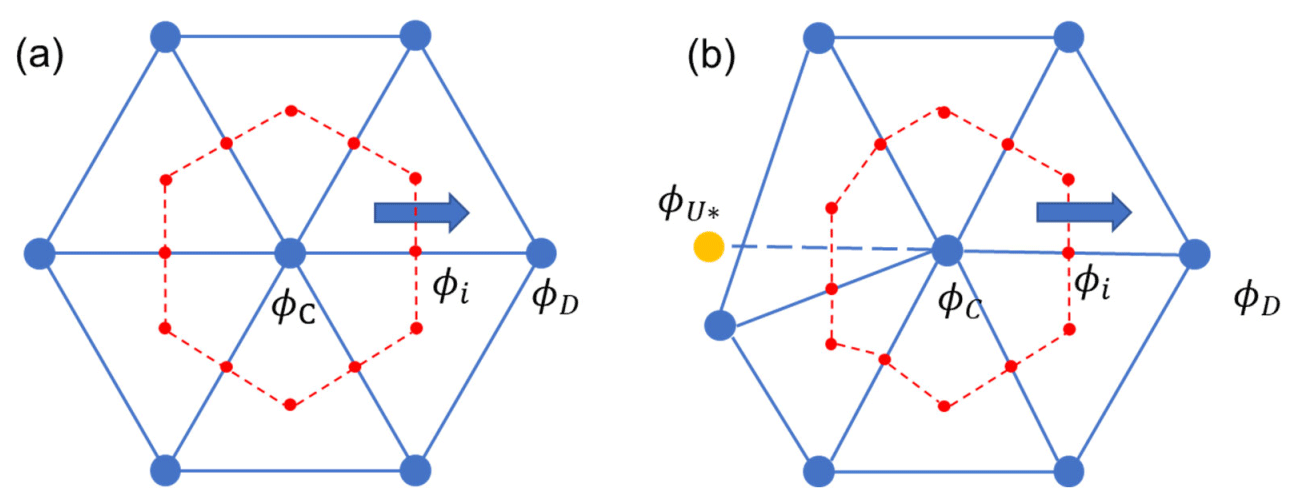
Figure 1 Schematics of control volume for the ice transport; (a) is for a uniform unstructured mesh, and (b) is for a generic unstructured mesh.

As the sea ice concentration cannot exceed 1 or be negative in this pure advection step (but after the transport step, it can exceed 1 and lead to the ridging process; in the latter case, Icepack will perform clipping), Darwish's method (Eq. 8) can produce errors and needs to be limited:

$$\begin{array}{}\text{(9)}& {\mathit{\varphi }}_{\mathrm{U}\ast }=min\left(\mathrm{1},max\left(\mathrm{0},{\mathit{\varphi }}_{\mathrm{D}}-\mathrm{2}{\mathit{R}}_{\mathrm{CD}}\cdot \left(\mathrm{\nabla }{\mathit{\varphi }}_{\mathrm{C}}\right)\right)\right).\end{array}$$

Using the approximation of edge values ϕ_i, we can calculate the sea ice area fluxes across every edge of the control volume and thus the new concentration from Eq. (3). Other tracer fluxes like volume per unit area of ice and enthalpy depend on the area fluxes, as in CICE. For instance, the volume per unit area of ice v_n equals the product of the sea ice area a_n and the sea ice thickness h_n; here h_i is the sea ice thickness of the upwind node.

$$\begin{array}{}\text{(10)}& {\displaystyle }{v}_n=a_n{h}_n,\text{(11)}& {\displaystyle }{v}_n^{t+\mathrm{1}}=v_n^t+{\displaystyle \frac{\mathrm{\Delta }t\sum _{i\in S}{Q}_i{\mathit{\varphi }}_i{h}_i}{{\mathrm{\Omega }}_S}}.\end{array}$$

Sea ice enthalpy e_n is the product of the sea ice area a_n, the sea ice thickness h_n, and the energy per unit volume q_n, here q_i is the energy per unit volume of the upwind node.

$$\begin{array}{}\text{(12)}& {\displaystyle }{e}_n=a_n{h}_n{q}_n,\text{(13)}& {\displaystyle }{e}_n^{t+\mathrm{1}}=e_n^t+{\displaystyle \frac{\mathrm{\Delta }t\sum _{i\in S}{Q}_i{\mathit{\varphi }}_i{h}_i{q}_i}{{\mathrm{\Omega }}_S}}.\end{array}$$

Other tracers at the new step can be calculated this way.

The finite-volume method ensures both global and local conservation of tracers. Since all ice area fluxes are recorded, the method requires only a single flux calculation per ice category, enhancing computational efficiency. Numerous tests have demonstrated that the TVD scheme provides second-order accuracy in smooth regions (D. Zhang et al., 2015) and guarantees strict monotonicity and good accuracy. The limiter for this study is the widely used van Leer limiter. Even though the accuracy of this limiter may be locally reduced to first order, it always maintains monotonicity as long as the time step used satisfies the stability condition, as demonstrated by Sweby (1984). Sea ice concentration can exhibit new extremes after the transport step as a result of physical processes such as convergence and divergence. Furthermore, the monotonicity of tracers is guaranteed because the method in Eqs. (11) and (13) is essentially a weighted average method with non-negative weights. And in general, the exchange caused by advection is relatively small in amount, i.e., $a_n^t\gg \frac{\mathrm{\Delta }t\sum _{i\in S}{Q}_i{\mathit{\varphi }}_i}{{\mathrm{\Omega }}_S}$, so the non-negativity of $a_n^{t+\mathrm{1}}$ is guaranteed. When we consider a divergent flow, h_i in Eq. (11) is just equal to h_n (the center node value) and here is

$$\begin{array}{}\text{(14)}& v_n^{t+\mathrm{1}}=a_n^t{h}_n+{\displaystyle \frac{\mathrm{\Delta }t\sum _{i\in S}{Q}_i{\mathit{\varphi }}_i}{{\mathrm{\Omega }}_S}}{h}_n,\end{array}$$

which is always non-negative.

3 Results

3.1 Idealized test case

Since the thermodynamic and dynamic parts of this model are relatively mature and have been widely utilized in other models, in this study we focus on validating the new transport scheme. The comparison of several transport schemes is carried out through an idealized ice transport experiment in a uniform unstructured mesh. The mesh grid consists entirely of equilateral triangles, with a side length of 200 m for each triangle. As the initial condition, we placed a rectangular sheet of sea ice with dimensions of 5000 m × 5000 m on the left side of the mesh. The initial ice thickness is 1.5 m, and it moves to the right along the x axis at a speed of 1 m s⁻¹. The time step is 1 s, which satisfies the Courant–Friedrichs–Lewy (CFL) condition for TVD and meets the stricter CFL condition for SCHISM (Z. Zhang et al., 2016). We run the idealized experiment for 24 h, equivalent to 86 400 steps. We select two other second-order transport schemes for comparison: the second-order upwind scheme referred to as UG-CICE (Gao et al., 2011) and the FEM-FCT scheme. It should be noted that in UG-CICE, although tracers are positioned at vertices (nodes) as in our model, the velocity is calculated at the centroids, differing from our scheme. The skill metrics employed include the accuracy and the monotonicity of the results.

3.1.1 Accuracy

Figure 2 shows the snapshots and corresponding central profiles along the x axis of the sea ice concentration taken every 3 h, with the theoretical solution represented by the red rectangles. For clarity, only areas with a concentration greater than 15 % are shown, and to show more details, only the first three and last three snapshots are shown. Compared to other schemes, the second-order upwind scheme exhibits significantly higher diffusivity but is relatively uniform. The shape of the ice distribution varies over time, transitioning from a square to a circle. By the conclusion of the model run, the peak ice concentration is reduced to roughly 20 % of its initial value – this is the lowest retention observed amongst the three schemes. Moreover, most nodes fall below the 15 % concentration visibility threshold in the snapshot. The FEM-FCT scheme retains most sea ice in the red rectangle, while it produces a banded distribution at the trailing and leading edges (Fig. 2b). The profiles portrayed in Fig. 2e indicate that the peak of sea ice concentration consistently approaches 100 % and is the sharpest result of the three schemes. Figure 2c and f demonstrate that the TVD scheme matches the FEM-FCT's accuracy better than that of the second-order upwind scheme. Moreover, the horizontal distribution of the ice is also close to the analytical solution and exhibits a peak ice concentration around 100 % at all times, despite some diffusion at the frontal edges, akin to the FEM-FCT scheme.

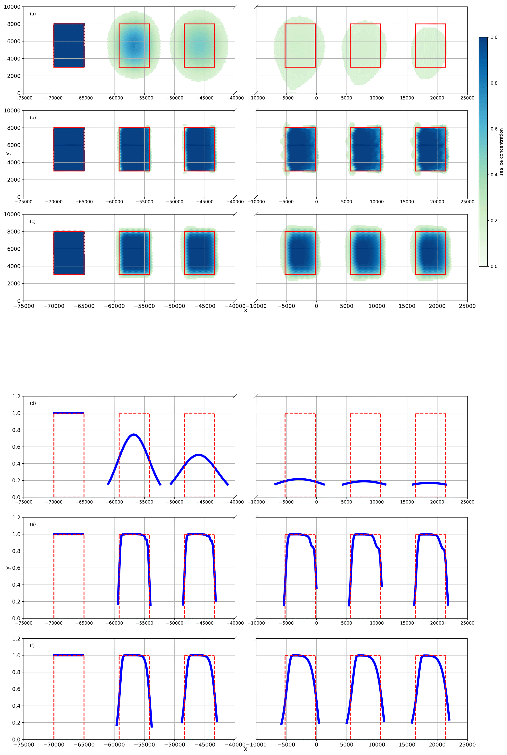
Figure 2 Sea ice concentration snapshots (a–c) and profiles (d–f). The sea ice moves from left to right, snapshots are taken every 3 h, and the red rectangle is the exact solution. (a, d) Second-order upwind, (b, e) FEM-FCT, and (c, f) TVD. To show more details, only the first three and last three snapshots are shown.

The results of the ice volume per unit are analogous to the patterns observed in ice concentration (Fig. 3). Among the tested schemes, the second-order upwind scheme is the most diffusive one, with a peak of ice volume per unit area of only 0.3 m at the end. The FEM-FCT and TVD schemes both demonstrate comparable accuracy, maintaining the shape and its peak value. From commencement to conclusion, the geometries of the ice volume per unit area closely resemble the theoretical model, with the peak values for TVD (1.496 m) and FEM-FCT (1.495 m) finishing marginally below the precise solution. The ice volume per unit profiles of the three schemes (Fig. 3d–f) exhibit shapes analogous to those seen in the ice concentration (Fig. 2d–f), suggesting all schemes largely preserve monotonicity. However, the FEM-FCT scheme exhibits non-monotonic behavior at the ice edges, and this will be further discussed below.

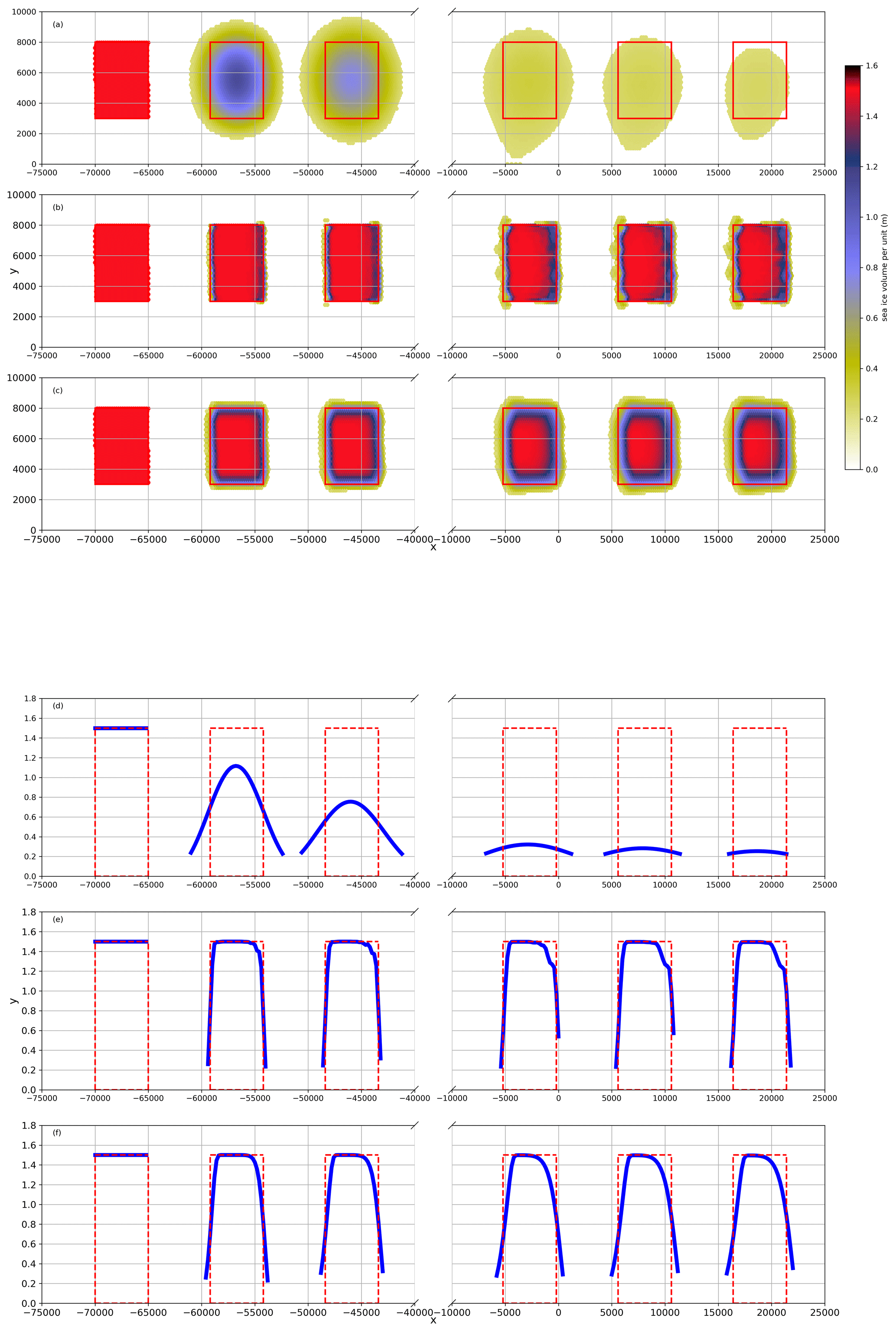
Figure 3 Volume per unit area of ice, with snapshots (a–c) and profiles (d–f). The sea ice moves from left to right, snapshots are taken every 3 h, and the red rectangle is the exact solution. (a, d) Second-order upwind, (b, e) FEM-FCT, and (c, f) TVD. To show more details, only the first three and last three snapshots are shown.

3.1.2 Monotonicity

Here we select the ice thickness as representative of tracers to verify monotonicity, with the ideal transport scheme expected to maintain the initial ice thickness (1.5 m). Figures 2d and 3d show that the second-order upwind is overly diffusive, so we exclude it in the current comparison. Considering that non-monotonicity typically occurs in areas of low ice concentration, we choose 0.1 % as the threshold rather than the previous 15 %. In most areas, the FEM-FCT scheme maintains monotonicity, and the ice thickness remains consistent with the initial value (Fig. 4a). But at the leading edge of the ice, the thickness overshoots the initial value and oscillates at the trailing edge. For the TVD scheme, some overshoots would occur at the leading edge of ice (Fig. 4b) if we did not limit the up-upwind value (see Eq. 8). On the other hand, the modified TVD scheme we developed that limits the up-upwind value (see Eq. 9) is completely monotonic (Fig. 4c).

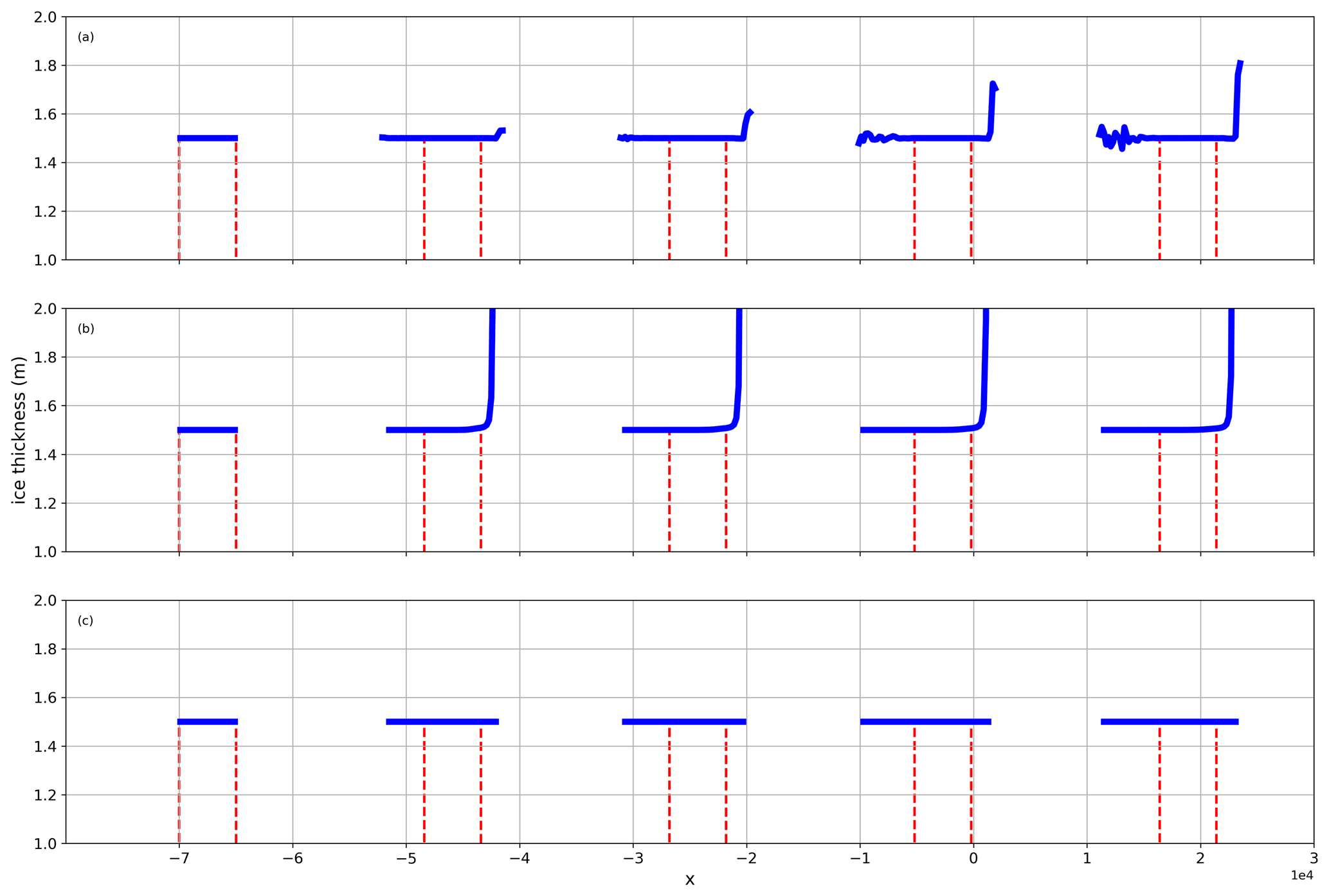
Figure 4 Sea ice thickness calculated from (a) FEM-FCT, (b) original TVD (Eq. 8), and (c) modified TVD (Eq. 9) for ice. The time interval of snapshots is every 6 h.

In summary, we have demonstrated that the TVD scheme provides second-order accuracy and outperforms that of the second-order upwind method. Although the FEM-FCT method could be more accurate than the TVD scheme, its propensity for non-monotonicity can cause numerical overshoots, consequently leading to unphysical values for the salinity or temperature of ice, which might result in model instabilities or even “blowup”. Approaches to enforcing the monotonicity in the FEM-FCT method may entail higher cost (Löhner et al., 1987) or lower accuracy (Zhang et al., 2023). On the other hand, the TVD scheme not only preserves the tracer monotonicity but also meets other requirements such as accuracy, and we will further test its efficiency in a realistic case.

3.2 Realistic model run

SCHISM–Icepack, in conjunction with the TVD scheme for its ice transport module, is employed to reproduce the ice processes in Lake Superior and the Arctic Ocean (Fig. 5). Successful tests on unstructured grids demonstrate the cross-scale capability of SCHISM–Icepack.

3.2.1 The Lake Superior case

To gauge the numerical efficiency of the new TVD scheme, we test it on a very fine-resolution Lake Superior mesh (Fig. 5a) that was previously used in Zhang et al. (2023). The nearshore resolution in this mesh reaches ∼ 50 m, with the finest resolution of 41.5 m found on the southwestern shore. As Zhang et al. (2023) indicated, the FCT scheme was having stability issues, so an essentially upwind method was applied in the high-resolution areas. The performance is compared with the upwind scheme. We simulate the case for 180 d from 1 December 2017 using 60 processors. The total simulation times for the two schemes are comparable: 678 min for the TVD scheme and 675 min for the upwind scheme. In total, the upwind scheme consumes 52.39 core hours, while TVD spends 54.56 core hours. Compared to the total time of the ice module, TVD accounts for 21.71 % and upwind accounts for 21.01 %, while the dynamic part is the most computationally intensive, accounting for more than 70 %. Overall, we found that the computational cost of the TVD scheme is comparable to that of the upwind scheme in this realistic benchmark application.

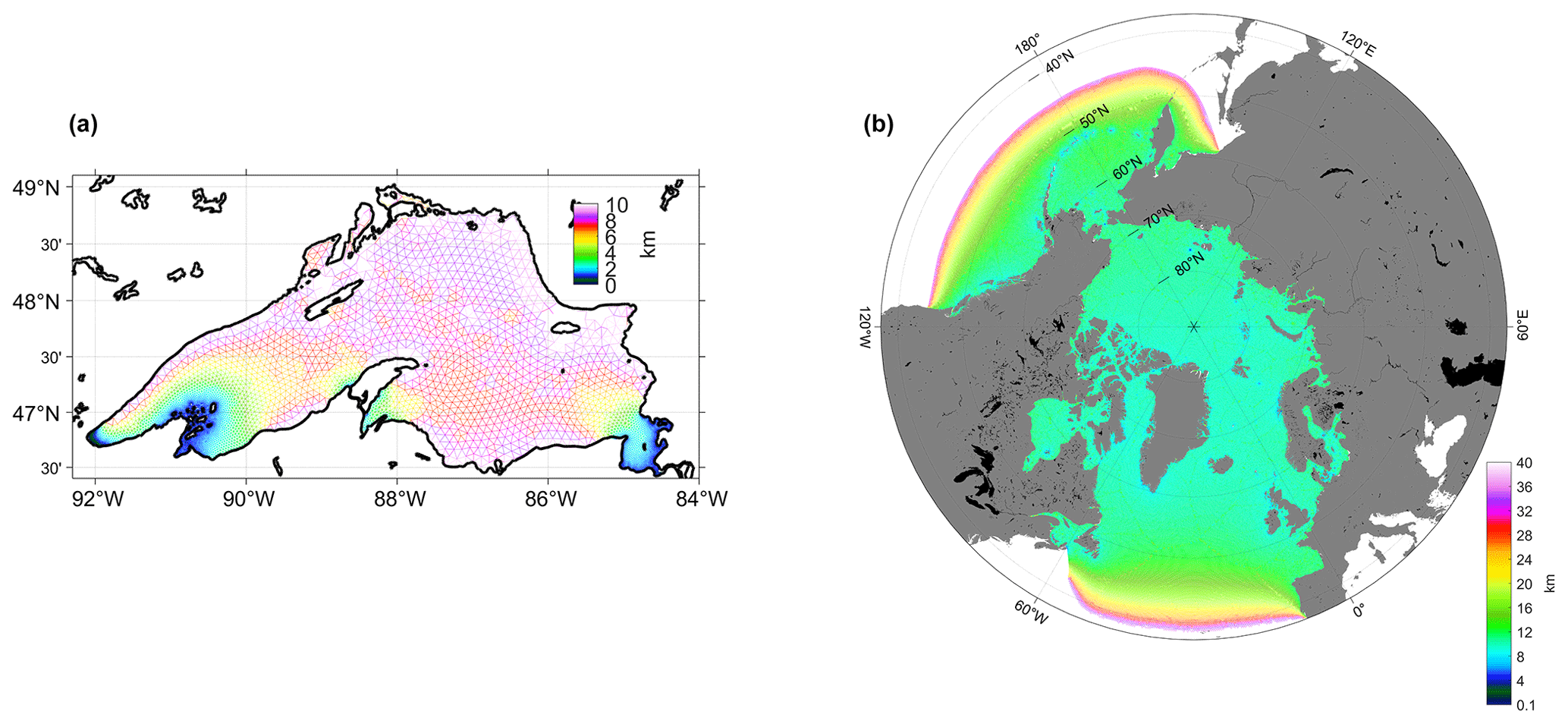
Figure 5 (a) The Lake Superior mesh. (b) The Arctic Ocean mesh. The colors show the mesh resolution.

As we mentioned before, Zhang et al. (2023) used a single-class ice model to reproduce the seasonal and interannual variability of ice extent (the ice concentration greater than 15 %) in this case. The simulation results have been compared to the Great Lakes Surface Environmental Analysis (GLSEA) (2024) data, including some rapid melting–refreezing events. But they also found in their model that ice melts excessively fast near the end of each melting season. Here we compare the ice extent and ice concentration between two models. With the multi-class ice model and the TVD scheme, we are able to reproduce the similar pattern of ice extent and also some rapid melting–refreezing events, yielding a correlation coefficient of 0.93 and a Wilmot score of 0.92 (both values being closer to 1 is better; Fig. 6). Furthermore, the melting phase simulation is improved beyond day 120. Approximately 10 000 km² of ice persists until around day 150 and the ice dissipates by day 160, aligning more closely with observational data. After the observed ice extent falls below 10 000 km², the correlation coefficient between simulated extent and observed extent with the multi-class ice model is 0.82, which is an improvement over the single-class ice model's coefficient of 0.43.

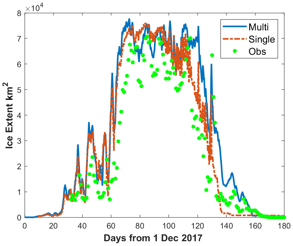
Figure 6 Comparison of ice extent in Lake Superior in 2017; the blue line is the result of the multi-class ice model, the orange line is the result of the single-class ice model, and the green dot is the observation from GLSEA.

The spatial distribution of the ice concentration from the two models is compared with the observation from the US National Ice Center (USNIC) on day 90 (Fig. 7), when the ice cover was largest. Both models exhibit lower ice concentrations in the southern part of the lake, while in most other areas, particularly in the western region, the multi-class ice model displays lower ice concentrations. Compared to the USNIC data, both models overestimate ice concentrations on the lake's eastern side. However, the multi-class ice model reproduces the ice-free pattern on the west coast more accurately. The spatial average ice concentration is 0.617 for the multi-class ice model, which is closer to the observed value of 0.509 and represents a significant improvement over the single-class ice model's 0.847. In the very high-resolution areas (the lake's southwestern and southeastern corners), the new coupled model and the TVD scheme yield a reasonable and stable result, which demonstrates its cross-scale capability.

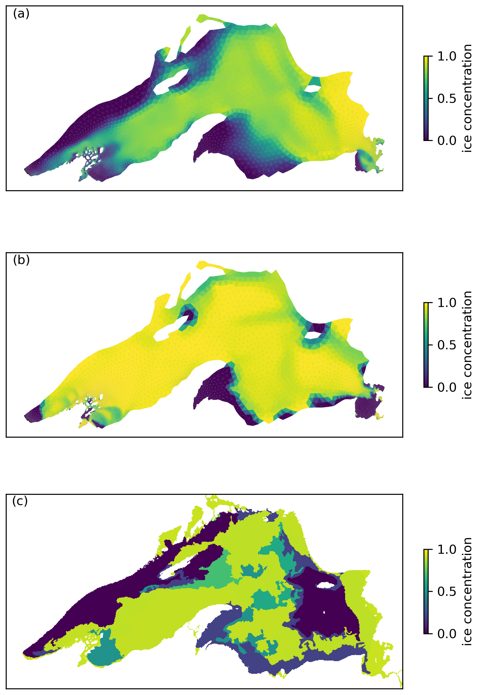
Figure 7 The ice concentration on day 90. Panel (a) is the result of the multi-class ice model and (b) is that of single-class ice model; (c) is from USNIC.

3.2.2 The Arctic Ocean case

The Arctic mesh consists of 422 000 elements and 217 000 nodes (Fig. 5b), with the resolution ranging from 6 km near the coast to 40 km at the open boundary. The model starts on 1 January 1994 and covers 2000 d, about 1.6 million steps, using a time step of 100 s. Initial conditions are derived from the HYCOM dataset, including ocean tracers as well as sea ice concentration and thickness. Moreover, the boundary conditions incorporate data from HYCOM and a finite-element solution (FES2014; Lyard et al., 2021), including 15 tidal components. The domain boundary is chosen to be at ∼ 40° N to ensure no sea ice crosses the boundary. In the vertical dimension, a highly flexible vertical gridding system (LSC²; Y. J. Zhang et al., 2015) is implemented with up to 60 layers in order to more accurately represent the complex topography of the Arctic Basin, and we set the bottom drag coefficient with a constant Manning coefficient of 0.0025. For the atmosphere forcing, we choose the European Centre for Medium-Range Weather Forecasts Reanalysis Fifth Generation global reanalysis (ERA5, Hersbach et al., 2020) due to its high temporal resolution and utilize the bulk aerodynamic model (Zeng et al., 1998) to get the surface fluxes, like latent and sensible fluxes. The turbulence closure scheme in the ocean model is the generic length-scale equation as k–kl (Umlauf and Burchard, 2003), and the horizontal transport in the ocean model is TVD² (Ye et al., 2016). The parameters used in the sea ice model basically follow the standard CICE configuration, including a constant air–ice drag coefficient (about 0.0016) and a constant ice–ocean drag coefficient (about 0.006). Modules in the standard CICE are also included in this model, such as the mushy layer thermodynamics, the Rothrock (1975) ice strength method, and the level-ice melt pond module among others. We evaluate our Arctic sea ice case by comparing its outputs to observational datasets from NSIDC, including the sea ice extent, ice boundary, and ice concentration. The observation of sea ice concentrations is from Nimbus-7 SMMR and DMSP SSM/I-SSMIS passive microwave data (Fetterer et al., 2017), while the sea ice boundary corresponds to the 15 % sea ice concentration contour.

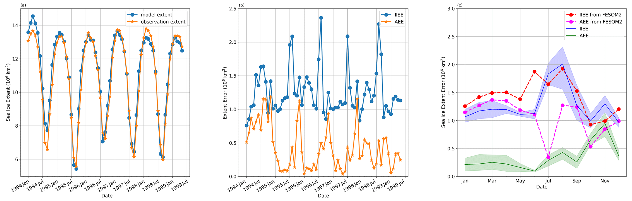
Figure 8 (a) Monthly sea ice extent of the model and observation in the Arctic Ocean. (b) Monthly integrated ice edge error (IIEE) and absolute extent error (AEE). (c) Monthly IIEE and AEE of SCHISM–Icepack and FESOM2 (averaged across all years), with the shading representing the 95 % confidence intervals.

Figure 8a compares the sea ice extent of SCHISM–Icepack with the observation. The model is stable for the long-term test and has good performance in reproducing the interannual variability and the seasonal cycle, with both the minimum and maximum sea ice extents being reproduced satisfactorily. The first peak is noticeably higher than the observed value, which may be influenced by the initial conditions as we did not get all tracers, such as sea ice salinity and enthalpy, from HYCOM. The extent difference between the model and observation is evaluated as absolute extent error (AEE, Eq. 14). However, AEE may underestimate the model error due to the cancellation between the overestimation (O) and underestimation (U). The integrated ice edge error (IIEE, Eq. 15) may be a preferable choice to evaluate the simulation result (Goessling et al., 2016; Zampieri et al., 2018).

$$\begin{array}{}\text{(15)}& {\displaystyle }\mathrm{AEE}=\left|\sum (\left|O\right|-\left|U\right|)\right|,\text{(16)}& {\displaystyle }\mathrm{IIEE}=\sum \left|O\right|+\sum \left|U\right|.\end{array}$$

We present the monthly AEE and IIEE in Fig. 8b, provide monthly statistics for them, and compare our results with those from FESOM2 in Fig. 8c. The FESOM2 team has run multiple cases to investigate the sensitivity of results to various forcing and model complexities and to select cases for our comparison that were also driven by ERA5 and based on a multi-class ice thermodynamics BL99 (Zampieri et al., 2021). IIEE and AEE (Fig. 8b) fluctuate in a fashion similar to the monthly extent in Fig. 8a. In Fig. 8a, the simulated sea ice extent often increases more rapidly during autumn compared to observed data, and it appears to more closely match observations in the remaining seasons. AEE shows a similar pattern, being relatively small in spring and summer and reaching its maximum in autumn. The magnitude of AEE is also similar to that of FESOM2, peaking in autumn while being lower in other seasons. The seasonal pattern of IIEE is similar to that of FESOM2, with maximum values during summer and lower values during autumn. Correspondingly, the largest variability of IIEE occurs in summer, while the lowest variability is observed in spring. The differences between SCHISM–Icepack and FESOM2 can be attributed to two primary factors: the first is that the selected FESOM2 results employed a different thermodynamic module, and the second is that the integration period of FESOM2 spanned from 2002 to 2015, while the integration period of this study is from 1994 to 1999. Nonetheless, the performance of the two models is generally comparable.

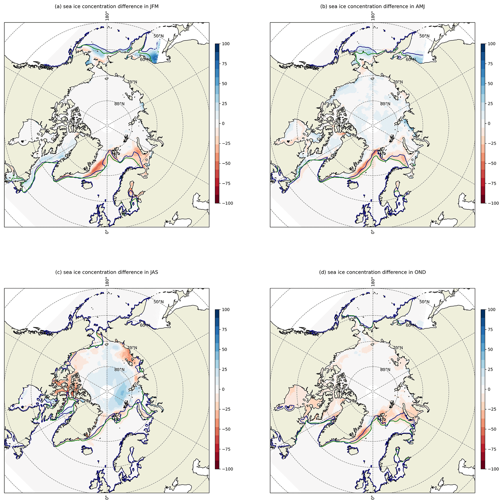
Figure 9 Seasonally averaged sea ice concentration difference (observation–model). The blue line is the satellite sea ice boundary, and the green line is from the model. (a) Winter (January, February, and March), (b) spring (April, May, and June), (c) summer (July, August, and September), and (d) autumn (October, November, and December).

The comparison of the spatial sea ice concentration is shown in Fig. 9. The simulated sea ice boundary and ice concentration show good agreement with satellite observations, and the model shows a robust ability to capture the seasonal evolution of sea ice in the Arctic Ocean. During winter and spring (Fig. 9a and b), deviation occurs in the marginal ice zone, such as the Bering Sea and the Greenland Sea. In summer (Fig. 9c), the model overestimates the sea ice concentration near the coast, such as the Canadian archipelago coast, but underestimates it in the central Arctic Basin. The overestimation is likely due to the model's simplified representation of complex thermodynamic and dynamic processes in the coastal margin (e.g., the occurrence of landfast sea ice). Furthermore, the lack of precise runoff and temperature data for Arctic rivers has a significant impact on the coastal area simulation. In the central Arctic Basin, melt ponds have a significant effect on the mass of sea ice during the melting season, and they are typically formed as a certain amount of precipitation remains on the ice (Feng et al., 2022). The precipitation field we utilized shows slight overestimation compared to the observation-based precipitation products (Marcovecchio et al., 2021), so it is plausible that the underestimation of sea ice concentration in the central Arctic Basin is caused by the excessive melt ponds that were reproduced in SCHISM–Icepack. In autumn (Fig. 9d), the model overestimates sea ice concentration in the marginal seas of the Arctic, such as Hudson and Baffin Bay, which causes the largest AEE. The heat exchange at the air–ice–sea interface is generally more intense in the freezing season compared to the melting season, so the coupled model may generate more sea ice due to its inability to deliver sufficient heat to the surface in time or due to the underrepresented strength of convection in the upper ocean.

The sea ice thickness is also validated. The observed ice thickness data, derived from upward-looking sonar sea ice draft measurements, were collected by submarines for the SCience ICe EXercise (SCICEX; National Snow and Ice Data Center, 1998). The in situ data are compared with the corresponding model values using a box plot in Fig. 10. The model results closely match the observations in April 1994, September 1997, August 1998, and April 1999, while the bias of the mean thickness is less than 0.6 m. Underestimation of the ice thicknesses happens in other months, with the bias of the mean thickness ranging from approximately 1.0 to 1.5 m. Specifically in the springs of 1994 and 1999 (April both years and May in 1999), the median thickness exhibits a bias of about 0.6 m, which is smaller than over half of the individual CMIP5 models during the same season, where median thickness biases exceed 1.0 m (Stroeve et al., 2014). Overall, SCHISM–Icepack demonstrates a robust capability to replicate both the observed seasonal and interannual variability of sea ice thickness.

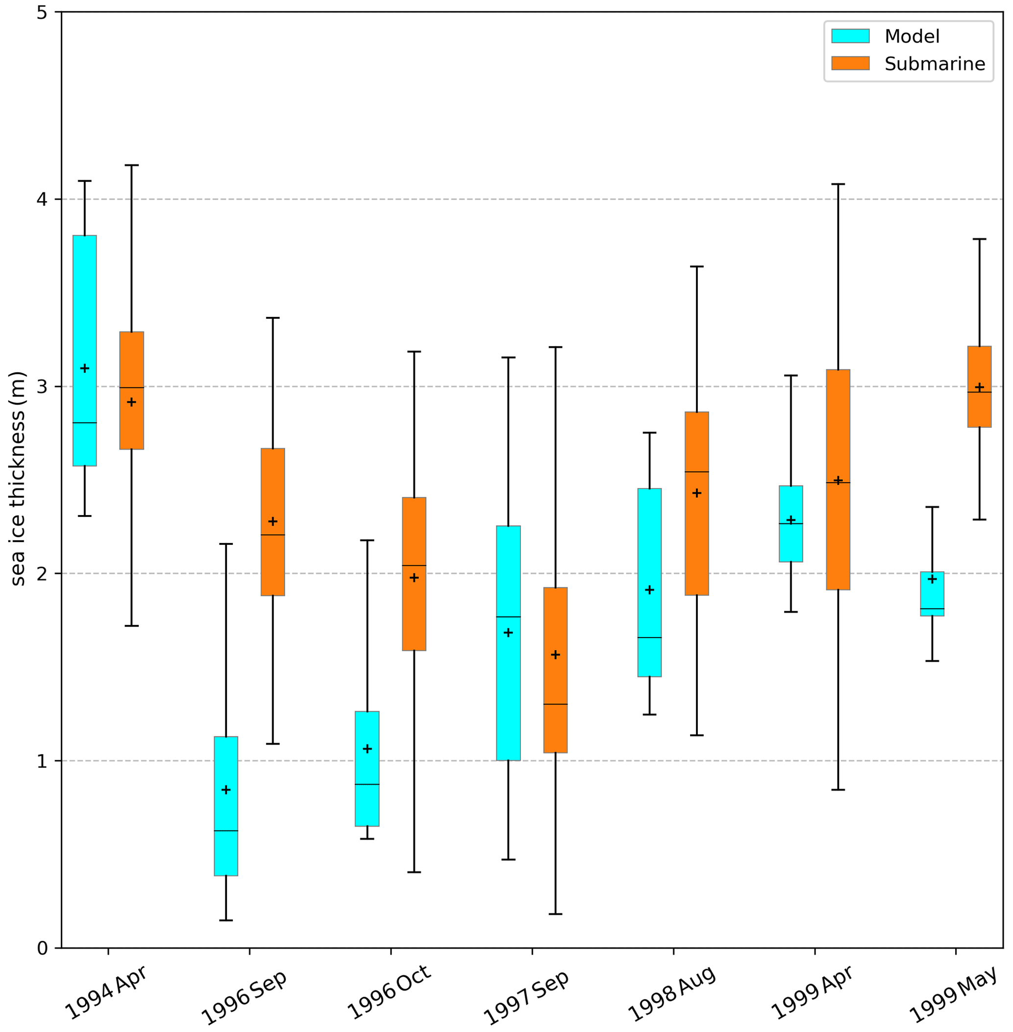
Figure 10 Box plot of sea ice thickness comparison. Cyan is the model result and orange represents the data from the submarine.

4 Conclusions

We have incorporated a multi-class sea ice module, the advanced sea ice column physics package Icepack, into the SCHISM modeling system. Significantly, we have implemented a new TVD-based scheme for ice tracer transport and validated it through an idealized case and realistic cases. The simulation results reveal that the TVD scheme is conservative, accurate, strictly monotonic, and efficient in reproducing the horizontal transport of ice, and it has better accuracy than the second-order upwind scheme at similar computational cost. Particularly, it provides strict monotonicity, which is crucial for stability, and thus addresses the difficulties encountered in the single-class ice model utilizing the FEM-FCT. The coupled SCHISM–Icepack model improves the results of the previous single-class ice model in the case of Lake Superior and was able to reproduce the Arctic Sea ice concentration, boundary, extent, and thickness as seen from the observation.

An advantage of the coupled model SCHISM–Icepack is its ability to effectively simulate the sophisticated ocean–ice evolution in both open-ocean and coastal regions. SCHISM includes various biogeochemistry modules like CoSiNE, while Icepack provides more detailed insights into the evolution of sea ice and biogeochemical processes. By integrating these biogeochemistry and physical modules in future work, we can deepen our investigation into the changes within under-ice ecosystems resulting from global warming.