Spurious numerical mixing under strong tidal forcing: a case study in the south-east Asian seas using the Symphonie model (v3.1.2)

The role of mixing between layers of different densities is key to how the ocean works and interacts with other components of the Earth's system. Correctly accounting for its effect in numerical simulations is therefore of utmost importance. However, numerical models are still plagued with spurious sources of mixing, originating mostly from the vertical advection schemes in the case of fixed-coordinate models. As the number of phenomena explicitly resolved by models increases, so does the amplitude of resolved vertical motions and the amount of spurious numerical mixing, and regional models are no exception to this. This paper provides a clear illustration of this phenomenon in the context of simulating the south-east Asian (SEA) seas along with a simple way to reduce its impact. This region is known for its particularly strong internal tides and the fundamental role they play in the dynamic of the region. Using the Symphonie ocean model, simulations including and excluding tides and using a pseudo-third-order upwind advection scheme on the vertical are compared to several reference datasets, and the impact on water masses is assessed. The high diffusivity of this advection scheme is demonstrated along with the importance of accounting for tidal mixing for a correct representation of water masses. Simultaneously, we present an improvement in this advection scheme to make it more suitable for use in the vertical. Simulations with the new formulation are added for comparison. We conclude that the use of a higher-order numerical diffusion operator greatly improves the overall performance of the model.

1 Introduction

Diapycnal mixing plays a fundamental role in the ocean, and precise quantification, localization and understanding of its mechanism are still active topics of research (Meredith and Naveira Garabato, 2022). Considering its major role in the heat uptake of the ocean, its correct representation in climate models is of utmost importance. Yet, a major flaw of ocean models is the tendency of numerical methods used to solve the equations on discrete grids to produce numerical errors, resulting in an excessive diffusion of tracer fields that is often referred to as “numerical mixing”. Considering the sensitivity of numerical model outputs to vertical mixing (Bryan, 1987), this spurious phenomenon becomes particularly troublesome when it occurs across isopycnals since there is less physical mixing in this direction than along the isopycnals, and numerical mixing can therefore easily dominate. In this context, the discretization of the vertical tracer advection equation in the fixed-coordinate model – regardless of whether they are terrain-following or geopotential coordinates – and the resulting spurious diapycnal fluxes have long been identified as a major source of spurious numerical mixing (Griffies et al., 2000), and this is still considered to be a major issue (Klingbeil et al., 2019).

Due to its advective origin, this spurious mixing is strongly linked to the strength of the flow and is therefore more sensitive in situations of strong vertical displacements. Even if “quasi-Eulerian” coordinates (Leclair and Madec, 2011) that vertically adjust with the motion of the free surface are now commonly used in ocean models, regardless of whether they are terrain-following or geopotential (see, for instance, Adcroft and Campin, 2004, for the adaptation to geopotential coordinates), therefore reducing the vertical velocity relative to the mesh, spurious mixing is still troublesome in the current class of global ocean models (Megann, 2018; Holmes et al., 2021). Besides, it might become even worse as the resolution increases and more physical processes are resolved explicitly – such as submesoscale and strong vertical speed anomalies associated with, for example, frontogenesis (Siegelman et al., 2020) or tides and the associated internal wave field, especially in regions of strong internal tide activity. In this sense, regional ocean models are particularly at risk, especially when run for long periods of time.

If the issue is known in the community of model developers, it is not certain whether the fast-growing community of model users is fully aware of this issue. Since the early 2000s, a number of studies have indeed focused on diagnosing spurious numerical mixing in idealized simulations (see, for instance, Burchard and Rennau, 2008; Klingbeil et al., 2014; Ilıcak et al., 2012; Gibson et al., 2017). However, the literature on spurious mixing in realistic simulations is still sparse (e.g. Lee et al., 2002; Megann, 2018; Holmes et al., 2021), is focused mainly on relatively coarse-resolution global models and relies on rather complex indirect estimates of mixing through water mass transformation analysis. Furthermore, none of the models used included explicit tidal forcing. Yet, owing to the advances in simulating tides in ocean models over the last few decades (see, for instance, Arbic, 2022) and the role they play in determining the global state of the ocean (Wunsch and Ferrari, 2004), more and more realistic simulations account for tidal forcing and the first few baroclinic modes are now routinely resolved in most regional applications. There is, therefore, a need to explicitly demonstrate the spurious numerical effect tides can have on tracer fields, even in relatively high-resolution models forced at their lateral boundaries. Also, though less precise, comparison against observations – made possible for instance by the growing number of Argo profiles in the ocean and the availability of high-resolution satellite products – and parameter sensitivity study can help to provide a clear picture of the effect of spurious mixing in realistic simulations.

Now, with the steady increase in available computing power, one can expect the spurious vertical mixing to eventually be reduced to acceptable levels (Holmes et al., 2021), especially since advection schemes are rarely of first order. The number of vertical levels has indeed increased by up to a factor of 10 over the last few decades. This, however, relies on the assumption that the range of vertical speeds resolved by the model does not depend too much on the vertical grid spacing. Furthermore, always increasing the resolution might not be desirable nor achievable in the foreseeable future for every research team and project around the world and therefore cannot be regarded as a definitive solution to the issue. Finally, the cost-effectiveness of an increase in resolution depends largely on the order of the schemes used, and both still have to be considered simultaneously (Sanderson, 1998).

Considering the fact that the issue of spurious numerical mixing generated by vertical advection is tightly linked to the (quasi-)Eulerian nature of fixed coordinates, moving toward more Lagrangian coordinates seems to have been the preferred option in recent years. Such approaches seem promising and have indeed demonstrated capabilities in reducing spurious diapycnal mixing (Gibson et al., 2017; Megann et al., 2022). In a recent paper, Megann (2024) demonstrated the ability of so-called $\stackrel{\mathrm{̃}}{z}$ coordinates (Leclair and Madec, 2011) to effectively reduce spurious numerical mixing in a global eddying simulation forced with tides. However, if they formally cancel the issue of spurious vertical mixing inherent to fixed-coordinate models, these approaches come at the cost of a whole range of new issues and limitations that remain a topic of active research owing to their relative youth (Fox-Kemper et al., 2019; Griffies et al., 2020). Moreover, their implementation into already existing numerical codes requires sustained effort by model developers over several years in order to be used in realistic simulations.

There is, therefore, a need for the expansion of the range of tools available for fixed-coordinate ocean models. The goal of this paper is twofold: a new, less diffusive formulation for advection schemes based on a scheme already implemented in the Symphonie model is proposed; validation of the method through the case study of simulations of the south-east Asian (SEA) seas is then proposed, providing a clear illustration of both the spurious numerical effect of tides in a regional model and their relevance in the accurate depiction of the region.

2 Model configuration

2.1 The south-east Asian seas

2.1.1 Regional context

Many locations have been shown to exhibit intense internal tide activity (Zaron, 2019), which is correlated with the existence of large areas of strong topographic gradients. Amongst them are the south-east Asian (SEA) seas (see Fig. 1), a large region of numerous deep marginal seas and shallow straits connecting the western Pacific to the Indian Ocean through an, on average, westward circulation known as the Indonesian Throughflow (ITF) (Sprintall et al., 2019). Due to this complex bathymetry, the region has long been known to be a hotspot of internal tide generation (e.g. Apel et al., 1985), and the dissipation of tides in the various semi-enclosed basins has been recognized as a major driver of the intensified mixing observed there (Ffield and Gordon, 1996). It leads to a sensible transformation of water masses on their way from the Pacific to the Indian Ocean, forming a unique water mass that can be tracked across the basin and beyond, up to the Agulhas Current (Gordon, 2005). This intensified mixing also acts as a cooling factor for the sea surface temperature (SST) in the region (Susanto and Ray, 2022) and modifies the atmospheric deep convection, which in turn impacts the regional and global climate (Koch-Larrouy et al., 2010; Sprintall et al., 2019). Interannual and climatic projections therefore need an accurate modelling of the ocean in the SEA region, and this cannot be achieved without an accurate representation of tidal mixing.

2.1.2 Modelling

On average, the vertical diffusivity over the region is indeed increased by more than 1 order of magnitude when compared with open-ocean estimates (Ffield and Gordon, 1992), with a high spatial variability (Purwandana et al., 2020), and it has been demonstrated in many studies that models not accounting for tide-induced mixing fail to correctly represent the water masses along the course of the ITF (Koch-Larrouy et al., 2007; Jochum and Potemra, 2008; Nugroho et al., 2018; Sasaki et al., 2018; Katavouta et al., 2022). Parameterization of tidally driven mixing has been successfully implemented in regional models (see, for instance, Koch-Larrouy et al., 2007) but still exhibits some weaknesses (Iskandar et al., 2023). Also, such an approach misses the dynamical effect of tides, which is suspected to play a non-negligible role in the horizontal mixing of water mass properties via the interaction of tidal currents with the complex topography of the region (Hatayama et al., 1996; Nagai et al., 2021), especially for high-resolution models. With the increase in computational capacities allowing for simulations to be run on finer grids, thus enabling the explicit resolution of more baroclinic modes, explicit tidal forcing is therefore being used more and more in regional models of the SEA region (Castruccio et al., 2013; Tranchant et al., 2016; Katavouta et al., 2022).

It must be noted, however, that most of the numerical codes used in those studies solve the primitive equations under hydrostatic assumptions. Considering the resolution of such large regional models, it is likely that this approximation remains valid insofar as non-hydrostatic phenomena such as small scales overturning are not resolved. Indeed, it is only possible to sense differences between hydrostatic and non-hydrostatic models when the model horizontal resolution is below a few tens of metres (see, for instance, Berntsen et al., 2009; Álvarez et al., 2019), and the advanced capability of such hydrostatic models forced explicitly by tides for reproducing in situ observations at a regional scale has been demonstrated in several studies (amongst others, see Tranchant et al., 2016; Katavouta et al., 2022; Thakur et al., 2022; Gonzalez et al., 2023; Bendinger et al., 2023).

Nonetheless, one may wonder how hydrostatic models actually represent tide-induced mixing. Formally, intensified mixing is achieved through the enhancement of the diffusivity computed by either the friction of tidal currents at the bottom or the turbulent closure schemes, such as k–ϵ, either through the buoyancy flux or the shear production terms (Gonzalez et al., 2023), and the results have been shown to compare reasonably well with specifically designed internal tide mixing parameterizations (see, for instance, Nugroho, 2017; Gonzalez, 2023, Chap. 5). However, the question of whether this is the fortunate result of several errors compensating for each other and if the existing models can actually capture the essential physical aspects of internal waves leading to mixing are still open – especially considering the fact that turbulent closure schemes, although based on first principles, were designed and calibrated at a time when internal tides were hardly resolved by ocean models. Still, such considerations, though of major interest for the community, are out of the scope of the present study, in which we will focus on numerical mixing.

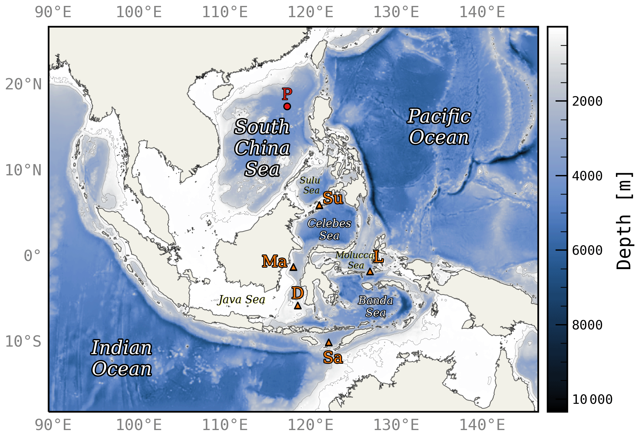
Figure 1 Bathymetry of the SEA configuration. The 100 and 1000 m isobaths are represented in fine grey lines. Locations Su, Sa, L, D and Ma correspond, respectively, to the Sulu Archipelago, the Savu Sea, the Lifamatola Passage, the Dewakang Sill and the Makassar Strait. Point P refers to the location of the profile, the evolution of which is shown in Fig. 3.

2.2 Model configuration and overview

The model employed in this study is the Symphonie ocean model (Damien et al., 2017, and references therein), a three-dimensional ocean circulation model that solves the primitive equations under Boussinesq and hydrostatic approximations. Symphonie has been used in the past over south-east Asia at several spatial scales, from the Gulf of Tonkin shelf scale (Piton et al., 2021; Nguyen-Duy et al., 2021) and south Vietnam upwelling coastal scale (To Duy et al., 2022; Herrmann et al., 2023) to the South China Sea regional scale (Trinh et al., 2024). Turbulent closure is achieved through the k–ϵ scheme (Burchard and Bolding, 2001). Integration in time is performed using a leapfrog time-stepping algorithm together with a Robert–Asselin filter to damp out spurious numerical modes. Barotropic and baroclinic modes are handled separately, following a mode-splitting procedure (Blumberg and Mellor, 1987). Momentum is advected via a fourth-order central differencing scheme along with an explicit biharmonic diffusion term, with a viscosity derived from the scheme developed in Griffies and Hallberg (2000). Since tracer advection schemes are the focus of this paper, the one used in Symphonie is discussed in Sect. 2.3.

Owing to the complex bathymetry of the region, equations are solved on a staggered Arakawa C-grid covering the entire south-east Asian region (see Fig. 1) using a rather high regular resolution of about 5 km on the horizontal. This resolution is relatively high compared to previous regional studies (Nugroho et al., 2018; Katavouta et al., 2022) and allows for a better representation of the many narrow straits in the region, especially along the Sunda Islands that separate the Indonesian seas from the Indian Ocean. To reduce truncation errors in sigma coordinates while maintaining an accurate description of the complex bathymetry, vanishing quasi-sigma (VQS) coordinates are used in the vertical (Dukhovskoy et al., 2009; Estournel et al., 2021), with 60 vertical levels. Since the coordinates are terrain-following, vertical resolution varies across the domain, ranging from around 2 m at the surface to up to 600 m on the last level at the deepest locations.

Currents and tracers are initialized using the $\mathrm{1}/\mathrm{12}$° × 50 fields from the Global Ocean Physics Reanalysis from the Copernicus Marine Service (GLORYS12V1, https://doi.org/10.48670/moi-00021, CMEMS, 2023a), hereafter called GLORYS, interpolated on our higher-resolution grid. Daily averages of temperature, salinity, sea surface height, and currents are then provided by the same model and applied at lateral boundaries. Tides are forced by M2, N2, S2, K2, K1, O1, P1, Q1 and M4 harmonics from the FES2014 tide atlas (Lyard et al., 2021). Along with the 5 km resolution, the configuration should be able to resolve between 80 % and 90 % of the barotropic-to-baroclinic conversion rate, following Niwa and Hibiya (2011), though the exact location of energy dissipation is still unclear. Surface fluxes are computed from the bulk formulae of Large and Yeager (2004) using variables from the European Centre for Medium-Range Weather Forecasts (ECMWF) operational forecasts at $\mathrm{1}/\mathrm{8}$° horizontal resolution and 3 h temporal resolution (https://www.ecmwf.int/, last access: 10 October 2023). In the region, 308 rivers are considered. Discharge flux time series are computed every 5 d and are derived from the 10 km resolution hydrological analysis GloFAS (Alfieri et al., 2013). More details on the practical implementation of rivers in Symphonie are provided in Nguyen-Duy et al. (2021), Appendix B.

Given the relatively low amount of validation data in the region (Sprintall et al., 2019), simulations have been chosen to coincide with the peak of Argo float profiles in the region and are therefore run for the 2017–2018 period. No Argo floats were indeed available in two major passages of the ITF before these years – namely, the Makassar Strait (linking the Celebes Sea to the Java Sea) and the Banda Sea. See Fig. A1 for locations of Argo floats in the region. Daily averages of each variable are saved for analysis. In total, four simulations have been run – T0, T1, NT0 and NT1 – the details of which are described in Sect. 3.

2.3 Advection

In the section that follows, we briefly describe the advection scheme used in Symphonie and the method implemented to improve the diffusive properties of the vertical component. We begin by describing the general framework in which the discussion is set and define the notation used. We then present the advection scheme that is already in use in Symphonie. Its numerical diffusivity is estimated and compared to physical mixing. A method is finally proposed to improve its diffusive properties and make it usable on the vertical.

2.3.1 Notation

As the issue we are dealing with arises from the vertical component of the tracer transport, we restrict our analysis to a one-dimensional situation and use notation considered standard for the vertical. We also make use of ℑ(⋅) and ℜ(⋅) to denote the imaginary and real parts of a complex number, respectively, and a circumflex, e.g. $\widehat{f}$ for a given operator f, is used to indicate the Fourier mode representation of a linear operator.

The continuous advection of a tracer $\stackrel{\mathrm{̃}}{s}$ by an incompressible flow of velocity field $\stackrel{\mathrm{̃}}{w}$ is expressed by the following equation:

$$\begin{array}{}\text{(1)}& {\partial }_t\stackrel{\mathrm{̃}}{s}=-{\partial }_z\left(\stackrel{\mathrm{̃}}{w}\stackrel{\mathrm{̃}}{s}\right).\end{array}$$

Tildes are used to distinguish continuous fields from their discrete counterparts. On a staggered regular grid {z_j} with constant spacing Δz, discretization of the equation in space in a finite-volume formulation for the discrete field s={s_j} advected by a velocity field w={w_j} is written as

$$\begin{array}{}\text{(2)}& {\displaystyle \frac{\mathrm{d}{s}_j}{\mathrm{d}t}}=-{\displaystyle \frac{(F_{j+}-F_{j-})}{\mathrm{\Delta }z}},\end{array}$$

where F_j+ (F_j−) conceptually represents the value of the flux field $F=\stackrel{\mathrm{̃}}{w}\stackrel{\mathrm{̃}}{s}$ at the interface between cells j and j+1 (cells j−1 and j). In such a formulation, w_j represents the velocity field $\stackrel{\mathrm{̃}}{w}$ sampled at location $z_j-\mathrm{\Delta }z/\mathrm{2}$, while s_j represents the tracer $\stackrel{\mathrm{̃}}{s}$ content in grid cell j, i.e.

$$\begin{array}{}\text{(3)}& s_j\left(t\right)={\displaystyle \frac{\mathrm{1}}{\mathrm{\Delta }z}}\underset{z_j-\mathrm{\Delta }z/\mathrm{2}}{\overset{z_j+\mathrm{\Delta }z/\mathrm{2}}{\int }}\stackrel{\mathrm{̃}}{s}(t,z)\mathrm{d}x.\end{array}$$

Hence, since F represents the flux at the interface, an estimate, s_j+, of $\stackrel{\mathrm{̃}}{s}(t,z_j+\mathrm{\Delta }z/\mathrm{2})$ will have to be reconstructed from the values of {s_j} via a given scheme. Advection schemes used in ocean models nowadays usually originate from standard interpolations procedures or weighted (often with non-linear weights) combinations of several other interpolations in order for the computed solution to satisfy certain desired properties.

Note that since quasi-Eulerian coordinates are used, the vertical velocity to be considered in practice in the discretization of the vertical advection is actually the Eulerian velocity $w_j^{\prime }$ – that is, the field obtained after removing the vertical displacements of the coordinates due to the movement of the free surface. Now, for large vertical displacements in the ocean interior that are caused, for instance, by strong internal tides, surface displacements are a few orders of magnitude lower than vertical displacements at a few hundred metres of depth, and the resulting difference between the true and relative fields is weak there. Thus, and since the theoretical framework used here is rather ideal, we use w_j although it might not be the perfectly accurate notation (or W when the velocity is considered constant) in the following to refer to this velocity relative to the grid points.

2.3.2 Advection of tracers in Symphonie

Horizontal advection of tracers is carried out using a pseudo-QUICKEST scheme, inspired by the QUICKEST scheme by Leonard (1979) that is hereafter referred to as QKE. Its flux formulation is formally written as follows:

$$\begin{array}{}\text{(4)}& F^{\text{QKE}}=(\mathrm{1}-(\mathrm{2}{n}_{\mathrm{c}}{)}^{\mathrm{2}})F^{\text{UP3}}+(\mathrm{2}{n}_{\mathrm{c}}{)}^{\mathrm{2}}{F}^{\text{UP1}},\end{array}$$

where n_c is the Courant number in the corresponding direction and F^UP1 and F^UP3 the fluxes for the first-order (UP1) and third-order (UP3) upwind advection schemes, respectively. Following Webb et al. (1998), the UP3 scheme is split into a fourth-order centred advection part (C₄) and a bi-Laplacian diffusive part (D₄), and the D₄ part is evaluated at time step t−1 during the leapfrog integration so as to ensure conditional stability. The UP1 part is fully evaluated at time step t−1.

The scheme behaves like a UP3 scheme for low Courant numbers, while for Courant numbers close to 0.5 (i.e. 2n_c∼1), the scheme turns into the forward integration of a first-order upwind discretization integrated with time step 2Δt, which is known to transport perfectly in those conditions. This hybrid behaviour increases the range of stability of the model and allows it to more robustly handle the few hotspots of strong Courant numbers. This scheme has demonstrated its robustness in the past applications of Symphonie, where vertical motions were either relatively low or the size of the domains allowed for a rapid regeneration of water masses by forcing at the boundaries, which are two assumptions that do not hold anymore in the present configuration.

Vertical advection of tracers in Symphonie is traditionally carried out with a second-order centred advection scheme. However, under strong vertical motions, dispersive errors can have spurious effects on the density field, especially in the long run (see, for instance, Griffies et al., 2000; Hecht, 2010), and some kind of numerical diffusion is therefore required to prevent small-scale density instabilities from developing by either introducing linear diffusion operators (often implicitly included in upwind formulations) or using non-linear limiting procedures such as total variation diminishing (TVD) schemes (Cushman-Roisin and Beckers, 2011) or their stronger version, flux-corrected transport (FCT) schemes (Zalesak, 1979), in order to enforce some kind of monotonicity in the evolution of the field. We opted for the first approach by building on a linear scheme that is already implemented in Symphonie and trying to improve its diffusive properties through a lightweight formulation to make it usable on the vertical at rather low additional computational cost.

2.3.3 Excessive diffusion on the vertical

We can simplify the analytical discussion by considering that along the vertical, Eq. (4) essentially boils down to the formulation of a UP3 scheme in the regions of interest of the model. Indeed, using a time step time step Δt=180 s $\approx \mathrm{2}\times {\mathrm{10}}^{\mathrm{2}}$ s and numerical values for internal tides of $W\approx {\mathrm{10}}^{-\mathrm{3}}$–10⁻⁴ m s⁻¹, Δz≈10¹–10² m, we get $n_{\mathrm{c}}\approx {\mathrm{10}}^{-\mathrm{2}}$–10⁻⁵, so that $n_{\mathrm{c}}\ll (\mathrm{1}-(\mathrm{2}{n}_{\mathrm{c}}{)}^{\mathrm{2}})\sim \mathrm{1}$ and the role played by the UP1 part can be neglected, at least in the ocean interior. Though of higher order than UP1, the UP3 scheme is nonetheless known to still be excessively diffusive (see, for instance, Madec et al., 2022).

To quantitatively illustrate this behaviour, we derive the dispersion relation for a single Fourier mode, $s_j\propto s_k{e}^{i(kj\mathrm{\Delta }z-\mathit{\omega }t)}$, linking ω to k and expressing how a given harmonic wave with wavenumber k evolves over time. In such a spectral framework, the diffusive aspect of a scheme is expressed by the addition of a damping term to the corresponding dispersion relation. More specifically, writing this dispersion relation in its canonical form, $\mathit{\omega }\left(k\right)=\mathrm{\Omega }\left(k\right)-i\mathit{\gamma }\left(k\right)$, with Ω and γ being real valued functions of k, the scheme is said to be diffusive when the damping coefficient, γ(k), that quantifies the typical time $\mathit{\tau }=\mathrm{1}/\mathit{\gamma }$ at which a given wavelength is being damped out, is strictly positive.

If the scheme can be split as the sum of a purely dispersive part, 𝒜[s]_j, and a purely dissipative part, 𝒟[s]_j, as follows:

$$\begin{array}{}\text{(5)}& {\displaystyle \frac{\mathrm{d}}{\mathrm{d}t}}\left[s_j\right]=\mathcal{A}[s{]}_j+\mathcal{D}[s{]}_j,\end{array}$$

it follows immediately that $\mathrm{\Omega }\left(k\right)=-\mathfrak{I}\left(\widehat{\mathcal{A}}\right(k\left)\right)$ and $\mathit{\gamma }\left(k\right)=-\mathfrak{R}\left(\widehat{\mathcal{D}}\right(k\left)\right)$, as the pure dispersion and pure dissipation assumptions ensure that both $\mathfrak{R}\left(\widehat{\mathcal{A}}\right[k\left]\right)$ and $\mathfrak{I}\left(\widehat{\mathcal{D}}\right[k\left]\right)$ are zero (see, for instance, Webb et al., 1998, or Soufflet et al., 2016, for more details).

Let us now focus more specifically on the damping coefficient obtained for the UP3 scheme. The full discretization of this scheme can be found in both Webb et al. (1998) and Marchesiello et al. (2009). Here, only its dissipative part, D₄, is needed, and it is written as follows:

$$\begin{array}{}\text{(6)}& {\text{D}}_{\mathrm{4}}[s{]}_j={\displaystyle \frac{\mathrm{1}}{\mathrm{12}}}{\displaystyle \frac{\left|W\right|}{\mathrm{\Delta }z}}(-s_{j+\mathrm{2}}+\mathrm{4}{s}_{j+\mathrm{1}}-\mathrm{6}{s}_j+\mathrm{4}{s}_{j-\mathrm{1}}-s_{j-\mathrm{2}}).\end{array}$$

Replacing each s_j instance by its Fourier mode value, assuming the vertical speed W to be constant for the sake of simplicity and using the normalized form, θ=kΔz, for the wavenumber, we have

$$\begin{array}{}\text{(7)}& \widehat{{\text{D}}_{\mathrm{4}}}\left(\mathit{\theta }\right)=-{\displaystyle \frac{W}{\mathrm{6}\mathrm{\Delta }z}}(\mathrm{3}+\cos \mathrm{2}\mathit{\theta }-\mathrm{4}\cos \mathit{\theta }).\end{array}$$

This finally leads to the most compact form of the damping coefficient:

$$\begin{array}{}\text{(8)}& {\mathit{\gamma }}^{\text{UP3}}\left(\mathit{\theta }\right)={\displaystyle \frac{W}{\mathrm{3}\mathrm{\Delta }z}}(\mathrm{1}-\cos \mathit{\theta }{)}^{\mathrm{2}}.\end{array}$$

For the largest wavelengths, i.e. θ→0, we have γ^UP3(θ)→0, which is expected since we do not want the largest scales to be damped out, while for the smallest wavelengths, i.e. θ→π, the damping is maximal and equal to $\frac{\mathrm{4}W}{\mathrm{3}\mathrm{\Delta }z}$; the smallest, noisy wavelengths are damped out. Comparing this to the damping coefficient obtained for the simplest physical diffusion term, κ∂_zzs, with κ being the vertical diffusion coefficient computed from the turbulence closure scheme, discretized in its usual form, $\mathit{\kappa }(s_{j+\mathrm{1}}-\mathrm{2}{s}_j+s_{j-\mathrm{1}})/(\mathrm{\Delta }z{)}^{\mathrm{2}}$, that leads to the following physical damping coefficient:

$$\begin{array}{}\text{(9)}& {\mathit{\gamma }}^{\text{phy}}\left(\mathit{\theta }\right)={\displaystyle \frac{\mathrm{2}\mathit{\kappa }}{\mathrm{\Delta }{z}^{\mathrm{2}}}}(\mathrm{1}-\cos \mathit{\theta }).\end{array}$$

The ratio of numerical to physical damping, ${\mathrm{\Gamma }}_{\text{UP3}}={\mathit{\gamma }}^{\text{UP3}}/{\mathit{\gamma }}^{\text{phy}}$, is written as

$$\begin{array}{}\text{(10)}& {\mathrm{\Gamma }}_{\text{UP3}}={\displaystyle \frac{W\mathrm{\Delta }z}{\mathrm{6}\mathit{\kappa }}}(\mathrm{1}-\cos \mathit{\theta })={\displaystyle \frac{P_e}{\mathrm{6}}}(\mathrm{1}-\cos \mathit{\theta }),\end{array}$$

where P_e is the grid Péclet number. Typical values of P_e found in the model can be obtained using the same numerical values as before and considering a value of $\mathit{\kappa }\approx {\mathrm{10}}^{-\mathrm{5}}$ m² s⁻¹ typical of vertical diffusivity in the ocean interior (e.g. Polzin et al., 1997; Alford et al., 1999). This leads to P_e≈10²–10⁴. For intermediate wavelengths, $N=\mathrm{2}\mathit{\pi }/\mathit{\theta }$, of 10 grid points – that is, $\mathit{\theta }=\mathrm{2}\mathit{\pi }/\mathrm{10}$ – which is the typical number of grid points used to represent a thermocline, we then have Γ_UP3≈3–300. This means that the numerical mixing resulting from the discrete vertical advection is at least 3 times larger than the physical mixing at this scale, even under relatively conservative assumptions about the quantitative values, and can even be 2 orders of magnitude larger. The numerical diffusion is thus not selective enough, in the sense that it spuriously damps physical scales. In the section that follows, we propose a method to improve this selectivity.

2.3.4 Filtered diffusion

As discussed previously, UP3 can be written as the sum of a purely dispersive (C₄) and a purely dissipative (D₄) component. Since the damping originates from D₄, we now aim at making this term more scale-selective. This can be achieved through a filtering process: assuming a high-pass filter Φ that applies on the tracer field s, the idea is to apply the diffusive operator to the filtered field only, i.e. turn D₄[s] into D₄[Φ[s]], so that only the high spatial frequencies (smaller scales) are dissipated. In spectral space, since D₄ is linear, the damping coefficient for this scheme formally becomes

$$\begin{array}{}\text{(11)}& \mathit{\gamma }\left(\mathit{\theta }\right)=-\mathfrak{R}\left(\widehat{{\text{D}}_{\mathrm{4}}}\right(\mathit{\theta }\left)\right)\widehat{\mathrm{\Phi }}\left(\mathit{\theta }\right).\end{array}$$

Therefore, for large scales where $\widehat{\mathrm{\Phi }}\left(\mathit{\theta }\right)\sim \mathrm{0}$, γ(θ) will be almost zero, while for small scales where $\widehat{\mathrm{\Phi }}\left(\mathit{\theta }\right)\sim \mathrm{1}$, γ(θ) will remain unchanged. Here, we assumed $\widehat{\mathrm{\Phi }}\left(\mathit{\theta }\right)$ to be a real value, which is an assumption justified by the fact that it would otherwise introduce spurious lag in the filtered signal. Theoretically, many filters could fit. However, we now focus on the specific filter with which the method has been primarily developed and other formulations is discussed in Sect. 4. Inspired by a formalism proposed in Juricke et al. (2020b) in the context of the momentum equation, we define the filter $\mathrm{\Phi }=\mathbf{1}-\mathit{\varphi }$, where ϕ is a low-pass filter and 1 the identity operator. Formally, we rewrite the formulation of the UP3 as follows as what is hereafter referred to as the filtered formulation:

$$\begin{array}{}\text{(12)}& \text{UP3}\left[s\right]={\text{C}}_{\mathrm{4}}\left[s\right]+{\text{D}}_{\mathrm{4}}\left[s\right]-{\text{D}}_{\mathrm{4}}\cdot \mathit{\varphi }\left[s\right].\end{array}$$

Equation (11) then becomes

$$\begin{array}{}\text{(13)}& \mathit{\gamma }\left(\mathit{\theta }\right)=-\mathfrak{R}\left(\widehat{{\text{D}}_{\mathrm{4}}}\right(\mathit{\theta }\left)\right)(\mathrm{1}-\widehat{\mathit{\varphi }}(\mathit{\theta }\left)\right).\end{array}$$

Note that the original formulation of Juricke et al. (2020b) makes use of a more general filtering – namely, the following:

$$\begin{array}{}\text{(14)}& {\mathrm{\Phi }}_{\mathit{\alpha }}=\mathbf{1}-\mathit{\alpha }\mathit{\varphi },\end{array}$$

where α>0 is a parameter. α allows for the control of the strength of the filtering, α=0 corresponds to a no-filter situation, while α=1 corresponds to a fully active filter. The latter corresponds to our filtered formulation. The interesting aspect of the original formulation lies in the use of a value α>1. Such a regime could be interesting for the tracer equation, but since it comes with several issues, we restrict ourselves in this paper to the simpler case of α=1.

For our practical analysis, we introduce the three-point filter ${\mathit{\varphi }}_{\mathrm{3}}[s{]}_j=(s_{j+\mathrm{1}}+\mathrm{2}{s}_j+s_{j-\mathrm{1}})/\mathrm{4}$. Even though any low-pass filter can be chosen in theory, we have used this one for several reasons: it is the same as the one used in Juricke et al. (2020a); its simplicity allows for straightforward theoretical developments; and, finally, its limited stencil size does not increase the computational cost of the scheme too much (the full stencil size for computation of the advection term increases from seven to nine grid points), which may be desirable if the model is to be run over long time periods. This choice is further discussed in Sect. 4.

The filter's spectral representation writes ${\widehat{\mathit{\varphi }}}_{\mathrm{3}}\left(\mathit{\theta }\right)=(\mathrm{1}+\cos \mathit{\theta })/\mathrm{2}$. This leads to the following damping coefficient for the filtered UP3 scheme (hereafter UP3-F):

$$\begin{array}{}\text{(15)}& \begin{array}{rl}{\mathit{\gamma }}^{\text{UP3-F}}\left(\mathit{\theta }\right)& ={\displaystyle \frac{W}{\mathrm{3}\mathrm{\Delta }z}}(\mathrm{1}-\cos \mathit{\theta }{)}^{\mathrm{2}}(\mathrm{1}-{\displaystyle \frac{\mathrm{1}}{\mathrm{2}}}(\mathrm{1}+\cos \mathit{\theta }))\\ & ={\displaystyle \frac{W}{\mathrm{6}\mathrm{\Delta }z}}(\mathrm{1}-\cos \mathit{\theta }{)}^{\mathrm{3}}.\end{array}\end{array}$$

The relative damping for the filtered formulation ${\mathrm{\Gamma }}_{\text{UP3-F}}={\mathit{\gamma }}^{\text{UP3-F}}/{\mathit{\gamma }}^{\text{phy}}$ therefore becomes

$$\begin{array}{}\text{(16)}& {\mathrm{\Gamma }}_{\text{UP3-F}}={\displaystyle \frac{P_e}{\mathrm{12}}}(\mathrm{1}-\cos \mathit{\theta }{)}^{\mathrm{2}}.\end{array}$$

The comparison between γ^UP3 and γ^UP3-F is provided in Fig. 2. Considering again a wavelength of 10 grid points and using the same numerical values as before, we have ${\mathrm{\Gamma }}_{\text{UP3-F}}\approx \mathrm{0.3}-\mathrm{30}$. The damping at large scales as been reduced by 1 order of magnitude, and for the range of P_e of concern, the numerical dissipation can be now as high as or lower than the physical one. Numerical diffusion will now exceed physical diffusion where the vertical grid spacing is the coarsest – that is, at depth. Indeed, Δz=100 m is reached at 1000 m depth in our model, and at this depth, tracer profiles are already smooth enough so that their second- or higher-order derivatives are almost zero and diffusion, even numerical, is not really active at all. We therefore consider those values as a priori acceptable. Finally, the scheme used for the vertical tracer equation is referred to as the QKE-F scheme. The flux evaluation in Eq. (4) is thus finally modified as follows:

$$\begin{array}{}\text{(17)}& F^{\text{QKE}}=(\mathrm{1}-(\mathrm{2}{n}_{\mathrm{c}}{)}^{\mathrm{2}})F^{\text{UP3}-F}+(\mathrm{2}{n}_{\mathrm{c}}{)}^{\mathrm{2}}{F}^{\text{UP1}}.\end{array}$$

The Courant–Friedrichs–Levy (CFL) stability condition of the resulting scheme is not modified. Indeed, following Lemarié et al. (2015), the CFL constraint of the UP3 integrated as in our simulations using a leapfrog time-stepping scheme with Robert–Asselin filtering and a coefficient taken to be equal to 0.1 and lagging the evaluation of the diffusive term in time is n_c≤0.472. Using the same method, we can show that the constraint for UP3-F is n_c≤0.507. Since the UP1 term is lagged in time, it is as if it was integrated using a forward time-stepping scheme with time step 2Δt, and the CFL constraint for this term is 0.5, which is close to 0.472 and 0.507. Now, for n_c∼0.5, the UP1 term largely dominates in QKE and therefore sets the stability constraint, which is thus n_c≤0.5 for both QKE and QKE-F, as confirmed by a more formal stability analysis (not shown).

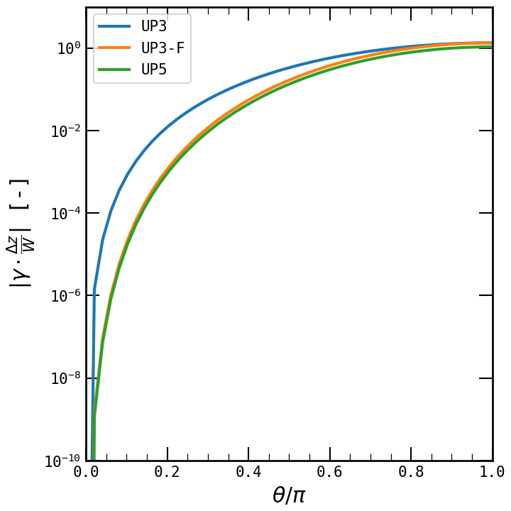
Figure 2 Comparison of the normalized damping coefficient $\mathit{\gamma }W/\mathrm{\Delta }z$ as a function of $\mathit{\theta }/\mathit{\pi }$ for several advection schemes. The y scale is logarithmic.

3 Results

A simplified one-dimensional framework such as the one presented above is essential for gaining insight into the actual behaviour of a numerical method (Griffies et al., 2000). However, this theoretical development relies on limiting assumptions intended to maintain analytical simplicity and, therefore, cannot be the only basis for designing practical advection schemes. This section provides a real case study for the validation of the method, illustrated as a way to improve water mass representation in simulations of the SEA seas using the Symphonie model. We start by briefly discussing the way spurious mixing is diagnosed in the model. A presentation of the results obtained from simulations with and without filtering is then presented and compared to their counterparts without tidal mixing. By doing so, we clearly illustrate the negative impact of numerical mixing and the improvement offered by our method in terms of representations of the water masses.

3.1 Diagnosing numerical mixing

Several frameworks for diagnosing numerical mixing have been proposed in the literature (e.g. Griffies et al., 2000; Lee et al., 2002; Burchard and Rennau, 2008; Gibson et al., 2017), each with their own strengths and weaknesses. These frameworks are, however, designed for inter-comparisons in a theoretical context of numerical methods for which the analytical computation of diffusion is not always possible, such as for non-linear schemes. As we focus here on the practical application of the method, we choose to proceed in a similar way as in Marchesiello et al. (2009) and to use anomalies in tracer fields (especially salinity, which exhibits a complex vertical structure with local maxima and minima) as a proxy for spurious mixing.

Several datasets are used for validation – namely, GLORYS reanalysis, Argo profiles (Wong et al., 2020), and OSTIA (Operational Sea Surface Temperature and Sea Ice Analysis) SST (Donlon et al., 2012) and SMAP/SMOS (Soil Moisture Active Passive and the Soil Moisture and Ocean Salinity missions) sea surface salinity (Kolodziejczyk et al., 2021) gridded products. Details on the data and processing are given when first used.

3.2 Effect of the QUICKEST scheme without the filtered formulation

To explicitly illustrate the excessive diffusivity of the QKE scheme on the vertical when used along with tidal forcing as well as the improvements brought by the filtered formulation, two reference simulations are first run with the filtered formulation turned off (α=0; equivalent to using QKE in its simplest formulation): one with tides (T0) and one without tides (NT0).

3.2.1 Salinity and temperatures profiles

Comparison to GLORYS data is first carried out to assess the ability of the model to maintain the salinity field in the South China Sea (SCS) over time (Fig. 3). Considering the higher availability of Argo floats in this basin (see Appendix A), it is assumed that GLORYS data offer a good and easy-to-handle reference for the state of the ocean. To allow for a more compact representation, the focus is placed on the 50–350 m layer, where differences between simulations are the most salient. Simply using the QKE scheme leads to an expected unrealistic erosion of the salinity maxima observed in Pacific waters in the northern South China Sea over the course of the first months of the T0 simulation (forced with tides). The salinity maximum of about 34.7 psu in the 100–200 m layer inherited from the initialization with GLORYS and visible at the very beginning of the simulation disappears to form a nearly isohaline profile below 100 m after a few months, with salinity below 34.6 psu. On the other hand, NT0 simulation is able to maintain the salinity peak comparable to the GLORYS reference value.

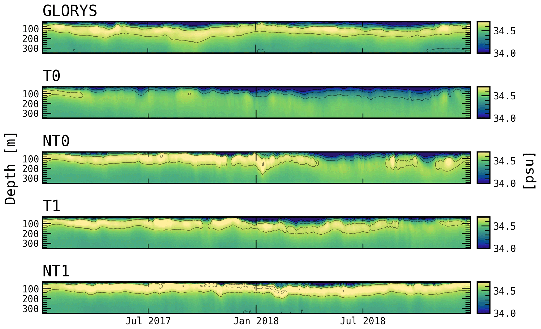
Figure 3 Temporal evolution of the salinity profile (50–350 m) averaged over a 1° box in the South China Sea at location P (as seen in Fig. 1) in both GLORYS reanalysis and several Symphonie simulations. Contours are plotted for every 0.2 psu.

Secondly, comparison of mean temperature and salinity profiles to Argo data available in the region over the period of interest are carried out (Fig. 4). For each simulation, a dataset of simulation profiles collocated to the Argo profiles in the zone – in terms of both space and time – is built. The profiles are split in several clusters that roughly correspond to the major basins sampled in the zone (see Fig. A1). They are then interpolated on the same grid over the first 500 m, and a mean profile is finally computed for each simulation and each cluster for comparison. The focus is placed on the first 500 m because this is where the temperature and salinity profiles exhibit their richest spatial structure and the ITF is mostly located in this layer. In Fig. 4, we only display profiles in the Molucca Sea for clarity (see Fig. 1) since the results in this basin are representative of the overall trend. However, the same analysis has been conducted in each basin of the region of south-east Asia and is discussed later on in the context of other simulations.

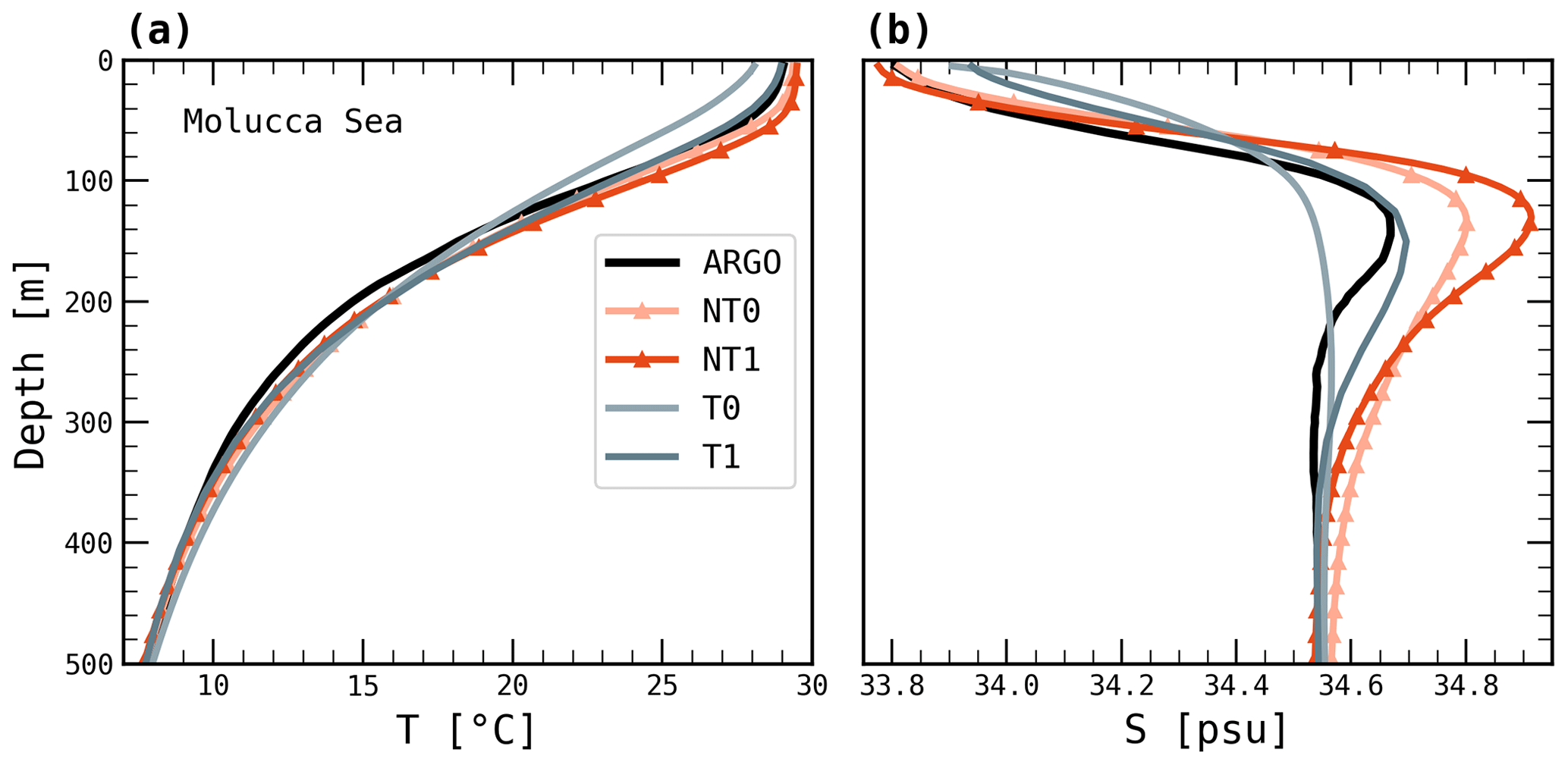
Figure 4 Mean (a) temperature and (b) salinity profiles over the first 500 m in the Molucca Sea for T0, NT0, T1 and NT1 simulations and Argo profiles.

As suggested by the drift observed for the South China Sea profile, the mean salinity between 100 and 300 m in T0 (Fig. 4b, light-grey line) is strongly underestimated with respect to Argo data, with a bias of around −0.15 psu at 125 m depth. The salinity maximum found between 100 and 200 m in observations and characteristics of Pacific waters has completely disappeared. In panel (a), the temperature gradient at 10–300 m depth is also slightly less steep, and the temperature in the upper 100 m in the T0 simulation also displays a negative bias of up to 2 °C at the surface.

Conversely, the salinity bias in the thermocline for the simulation without tides, NT0 (light orange), with respect to observations is positive, and the salinity maximum at 120 m is overestimated by about 0.1–0.2 psu. Differences in surface salinity are more complex to analyse and are discussed in more detail in Sect. 3.4. Differences in the temperature profiles are less obvious than for T0, even though a slight positive bias can be observed at the surface. Those differences result from an underestimation of physical mixing in NT0 that results in a misrepresentation of water masses in the region: as tides and the associated internal waves field are not taken into account, highly saline waters coming from the Pacific are not well mixed, which biases the model output.

3.2.2 Comparison to satellite sea surface temperature data

Finally, the OSTIA Level 4 Sea Surface Temperature daily product is also used for comparison. This product was obtained by mapping existing observations from several instruments on a regular $\mathrm{1}/\mathrm{20}$° grid with optimal interpolation and daily averaging results. Its resolution is therefore comparable in both space and time to our simulation's output. As with every highly processed product, care has to be taken not to put excessive confidence in such data since biases can exist, especially regarding small coastal features (see, for instance, To Duy et al., 2022). Large-scale trends are, however, well captured by OSTIA, and comparison is therefore carried out by computing the mean bias over the entire simulation period in the simulations and OSTIA. Results are displayed in Fig. 5. Since errors in the Pacific and Indian oceans are more likely caused by open-boundary forcing, the focus is placed on the interior basins, where most of the differences are concentrated.

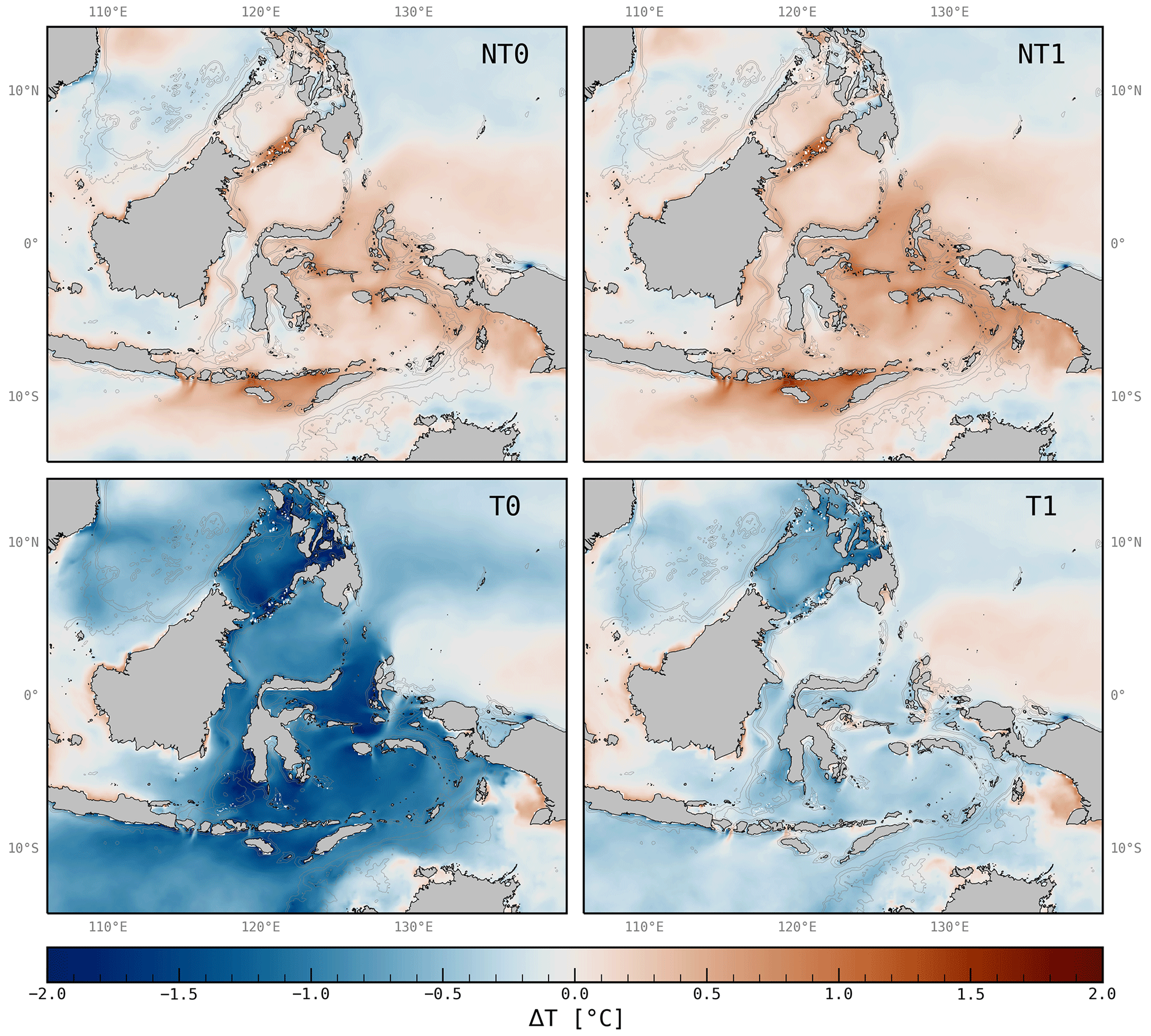
Figure 5 Mean SST bias with respect to the OSTIA dataset ($\mathrm{\Delta }\text{T}=\text{SST(SYMPHONIE)}-\text{SST(OSTIA)}$) for T0, NT0, T1 and NT1 simulations computed for the years 2017–2018. Positive values correspond to an overestimation in the model output. The 100, 500 and 1000 m isobaths are also displayed (fine grey lines).

A cold negative bias of up to 2 °C spans all Indonesian seas in simulation T0 (bottom-left panel), especially marked over the Savu Sea, the Dewakang Sill and along the islands south of the Sulu Sea (see Fig. 1 for details on the locations). Conversely, NT0 displays a warm positive large-scale SST bias of up to 1 °C with respect to the reference dataset, with maximum positive biases at the same locations where maximum negative biases are observed in T0. Both locations are known for being strong internal wave generation sites (Apel et al., 1985; Nagai and Hibiya, 2020) and exhibiting strong SST variations due to internal tide activity (Ray and Susanto, 2016). This confirms the conclusions obtained by examining salinity profiles: the (numerical) mixing is too strong in the presence of tides in T0, bringing colder water from below to the surface and thus cooling the simulated SST; conversely, the (physical) mixing is overly weak in NT0 due to the absence of tide-induced mixing and therefore prevents warmer surface waters to be mixed with colder waters at depth.

3.3 Effect of the QKE-F scheme

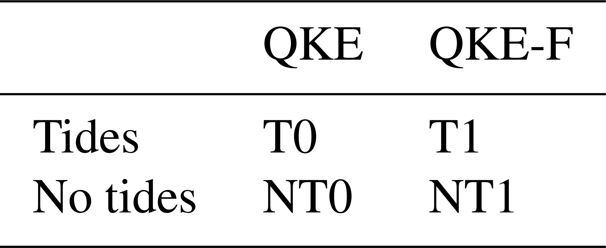
To assess the effect of the filtered formulation, two new simulations are run with the filtered formulation turned on (α=1): one including tides (T1) and its counterpart without tides (NT1). Differences to T0 and NT0 simulations in the same diagnostics as described above are presented in the following section. The main differences between the various simulations are summarized in Table 1.

Table 1 Summary of all the simulations run in this study along with their main differences. Columns correspond to the advection scheme used, i.e. either QKE or QKE-F, while rows indicate if tidal forcing was used or not.

3.3.1 Salinity and temperature profiles

Looking at the evolution of the salinity profile in the South China Sea in Fig. 3, the salinity maximum in T1 has been restored with respect to T0, and the evolution of the profile over the course of the T1 simulation lies much closer to not only the GLORYS reference dataset, but also NT0. This implies, first, that tides do not play a significant role in the (trans)formation of water masses at this location and, second, that the difference between T0 and NT0 is caused by the excessive numerical diffusion that occurs when tides are added. Concerning simulations without tides, the salinity evolution for NT1 depicted in Fig. 3 is also qualitatively better than for NT0, implying that there is still spurious mixing happening in NT0 in the South China Sea. This is to be expected since even simulations without tides can display transient, relatively high vertical velocities (on the order of a few tens of metres per day) and therefore spurious mixing, especially at eddy-resolving resolutions (see Megann et al., 2022).

Results in terms of mean profiles in the Molucca Sea are also reported in Fig. 4 for T1 and NT1. T1 performs better than T0 and overall follows the Argo reference more closely: the negative ∼ 1 °C temperature bias at the surface in T0 and the negative ∼ 0.1 psu salinity bias in thermocline waters disappear in T1. The implemented filtered formulation has thus effectively reduced the spurious mixing that develops in the context of strong tidal forcing down to acceptable levels. The picture is different for simulations without tides, i.e. NT0 and NT1. In terms of salinity, NT1 performs worse than the other simulations, even when compared to NT0, with an increased positive bias of 0.3 psu at 120 m depth compared to $\sim -\mathrm{0.15}$, 0.01 and +0.2 psu for T0, T1 and NT0, respectively. Tidal mixing indeed takes place in the Molucca Sea and drives the transformation of water masses (see, for instance, Koch-Larrouy et al., 2007). The weaker bias from NT0 in comparison to NT1 is due to the fact that the spurious numerical mixing in NT0 is higher than in NT1, thus making up for a part of the lacking tide-driven physical mixing. This again shows that even without tidal motions, a sensible amount of spurious mixing still takes place in NT0. With less numerical mixing in NT1, the underestimation of physical mixing is made all the more salient, which increases the bias and overestimation of the salinity maximum in NT1 compared to all other simulations.

To provide a more synoptic picture of the effectiveness of the filtered scheme, we carry out a comparison of all simulations in every basin of the zone. For a given simulation and zone, we define an integrated metric of the performances in terms of water mass representation to allow for a more direct and quantitative comparison than can be made solely through visual inspection. In each zone, a weighted root mean squared error between each simulation and the reference Argo profile is computed for the mean profile. As the variations in the upper layers are of higher magnitude than those in the deeper layers, we weight the error accordingly by reducing the importance given to values where the variation is higher. The resulting metric is referred to as wRMSE, and more details on its computation are provided in Appendix B. Here, the focus is placed on salinity as the effect of numerical mixing on these profiles is more obvious (see Fig. 4), but the same computations have been made for the temperature, yielding similar results (not shown).

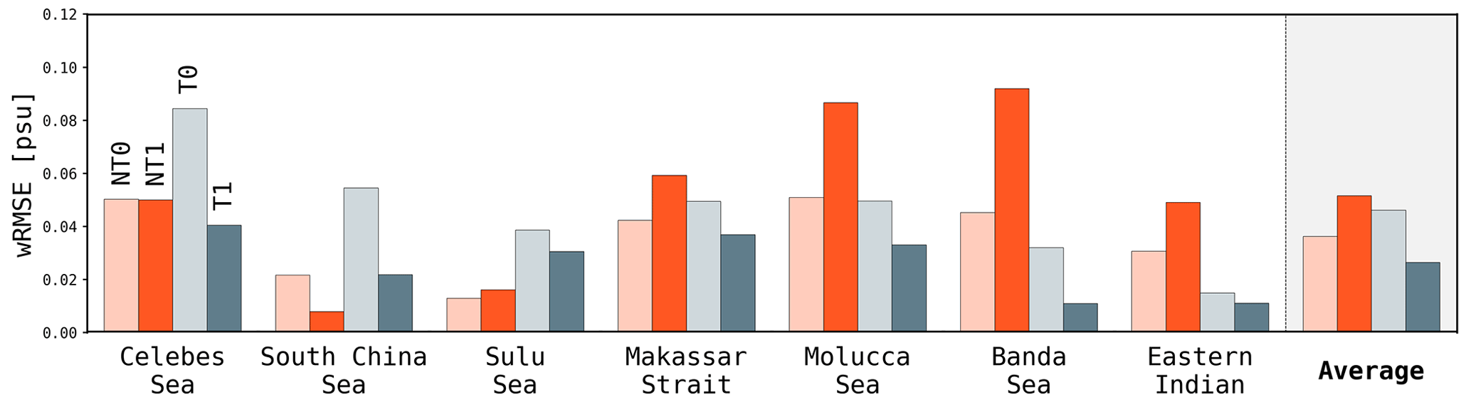
Figure 6 wRMSE between mean salinity profiles for T0, NT0, T1 and NT1 simulations (left to right bar for each zone, respectively) for each of the Argo subgroups. The last column displays the metric average for all zones.

The results of wRMSE computations on the salinity profiles for all simulation output for the various zones are displayed in Fig. 6. Values lie between 0.01 and 0.1 psu. Comparing the integrated wRMSE scores in the Molucca Sea with the profiles provided in Fig. 4, our metric indeed quantitatively translates the qualitative observation that in this zone, T1 performs the best and NT1 performs the worst, while T0 and NT0 are in between.

Comparison between T0 and T1 shows systematically improved wRMSE in T1 in each zone, with a much greater difference in zones that directly neighbour the Pacific (Celebes and SCS): around 0.04 psu in the SCS and only 0.01 psu in the Makassar Strait.

Except for the Sulu Sea, T1 also improves the results with respect to NT0. The difference is, however, usually smaller, except in the exit basins (Banda Sea and Indian Ocean) where the difference is sensible; wRMSE for T1 is 0.02–0.03 psu lower than for NT0 in those basins.

The performance of NT1 relative to the other simulations greatly varies with the location of the zone along the course of the ITF – that is, from the Pacific to the Indian Ocean through the Celebes Sea, the Makassar Strait and the Banda Sea. NT1 performances in the basins downwind of the ITF (Makassar Strait, Banda Sea, eastern Indian Ocean), where tidal mixing plays an important role, are by far the worse; there is around 0.08 psu between T1 and NT1 in the Banda Sea and 0.4 psu in the eastern Indian Ocean. However, in the SCS, NT1 performs better than all the others. The reason behind this best performance of NT1 in the SCS is still unclear and might be linked to some other factors, including the details of the configuration. Similarly, the best performances of NT0 and NT1 in the Sulu Sea are somewhat unexpected, and this feature is discussed below in the context of comparison to satellite data.

Figure 6 also displays the average wRMSE over all basins for each simulation, with a uniform weighting for each zone. Using this average metric, T1 performs overall best out of all simulations, while NT1 performs the worst. The wRMSE could have also been computed for each simulation by comparing the average profile for all available profiles over the ensemble basins to the same profile obtained with Argo data; however, this would have led the results to be strongly biased toward zones with the most data – in particular, the SCS. The underlying assumptions here are that the number of profiles available in each basin is sufficiently high, so comparisons can be trusted equally, and that the correct representation of each basin is of equal importance.

3.3.2 Comparison to sea surface temperature data

Finally, we also validate the filtered formulation against OSTIA SST data. The mean SST in T1 is greatly improved compared to T0 (Fig. 5): the negative bias over the SEA seas is lower by 1 order of magnitude and is now on the same order as errors made in the Pacific Ocean – that is, a few 10ths of a Celsius. This further confirms that our filtered formulation improves the representation of sea surface temperature in the context of strong tidal mixing.

The SST in the Sulu and Philippine seas, however, still exhibits a strong cold bias in T1 at up to 1 °C locally, which is weaker than in T0 but stronger than in NT0 and NT1. The explanation for this behaviour has been traced to an overestimation of tidal currents in this basin due to an imperfect representation of the numerous islands and channels around it, especially in the Philippine archipelago. Manual modification of the land mask to improve the representation of the zone was carried out, with sensible improvements when compared to the first tests, but tidal amplitudes remain too strong there. This results in an overestimation of the naturally strong internal tide activity in the area (Apel et al., 1985), which can only dissipate within the basin due to its enclosed nature, thus increasing the mixing. As a result, tidal vertical mixing is overestimated there, leading to spurious damping of the profiles and SST underestimation. This is slightly “corrected” when the filtering is activated (T1 vs. T0) and even greatly “corrected” when tides are turned off (NT0 vs. T0 and NT1 vs. T1).

Besides, the previously described positive SST biases in NT0 simulation shown in Fig. 5 are slightly increased in NT1, which is indicative of weaker vertical mixing in the interior basins – namely, along the Sulu island chain, the Savu Sea and around the Lifamatola Passage. Those results are again related to a reduction in spurious numerical mixing induced by the filtered scheme in NT1, whereas NT0 partly compensates for the lack of tide-induced physical mixing in NT0 and makes it more salient in NT1.

3.4 Non-linear effect of spurious numerical mixing on sea surface salinity

The results concerning numerical mixing presented so far – higher SST and strong erosion of the salinity maxima – can be explained within the simple framework of one-dimensional vertical diffusion, interpreting spurious numerical mixing as simply a higher diffusion, smoothing gradients and mixing properties throughout the column. In a realistic ocean model, however, many components interact, often in non-linear ways, and simple errors generated by one component can result in a priori unexpected behaviours. We briefly discuss an example of this in the case of air–sea interactions by comparing simulation output to sea surface salinity (SSS) products obtained from the SMOS and SMAP missions. The dataset used is the SSS SMOS/SMAP optimal interpolation (OI) L4 product, such as that described in Kolodziejczyk et al. (2021). Symphonie simulation output is downsampled at the same weekly frequency and interpolated on the same 25 km resolution grid. Results are displayed in Fig. 7.

A thorough discussion of all the biases in the region is out of the scope of this study, and we comment instead on the large-scale pattern. Overall, the bias is mostly lower than ±0.25 psu but can be locally increased to up to ±1 psu. A common pattern throughout all simulations is that several coastal regions exhibit large fresh biases, especially around Borneo, resulting from overestimated river discharges.

Differences between NT0 and NT1 are negligible and fall within the error margin of similar highly processed SSS products, especially in a region such as SEA, with its numerous islands and complex coastal features. Unlike for SST, which was overestimated in both of those simulations due to a lack of physical mixing, SSS bias does not exhibit any easily distinguishable patterns in simulations without tides.

As for simulations with tides, a large fresh bias spans the entire Indonesian seas region in T0 and is sensibly increased at locations of increased tidal mixing (locations Su, L and Sa as seen in Fig. 1), reaching negative salinity biases of up to 1 psu. This bias varies seasonally, with a large intensification of the pattern north of the Equator during boreal summer and south of the Equator for boreal winter (not shown).

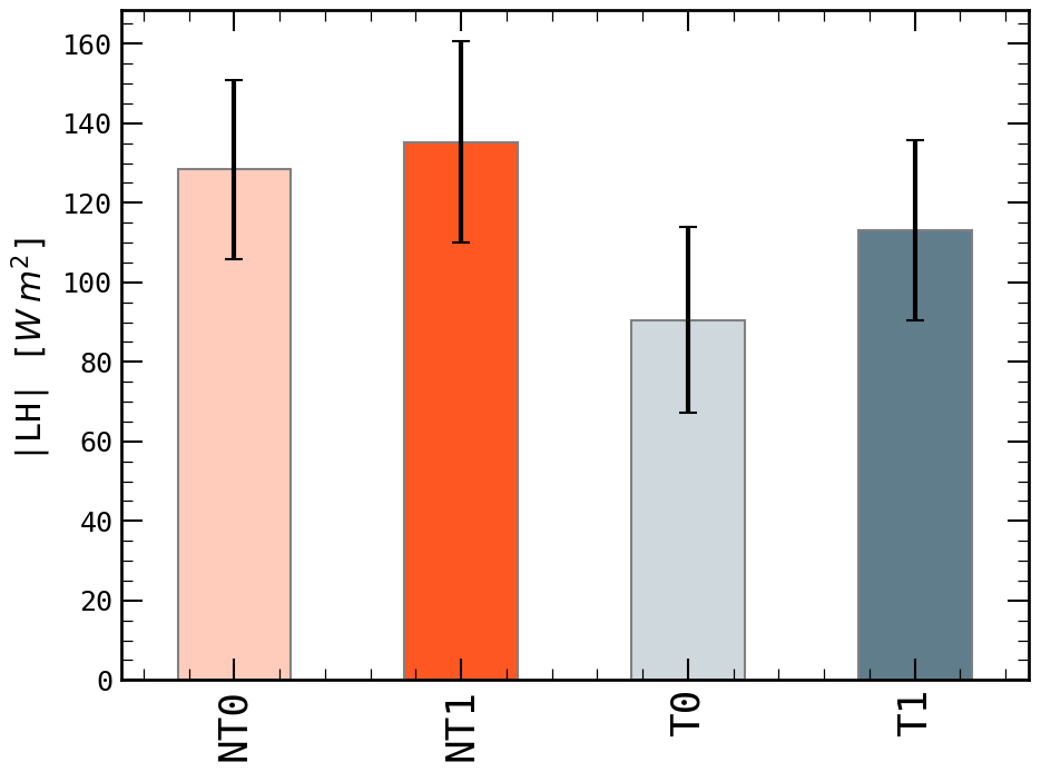
Those differences are in fact the result of the air–sea interactions. Since surface fluxes, including latent heat (LH) flux, are computed using bulk formulae, they adjust to the surface fields of the model – usually only SST – in a highly non-linear fashion notably caused by atmosphere stability considerations (see Large and Yeager, 2004). More precisely, the freshwater input at the surface in the absence of rivers is the difference between evaporation and precipitation. Precipitation is prescribed directly and does not change throughout the various simulations. Conversely, evaporation is proportional to the LH, which is itself a complex function of the forced atmospheric variables and the SST (which, as shown in Fig. 5, varies between the simulations). Mean values over the interior basins of LH as computed by the model for the various simulations are displayed in Fig. 8. Since LH is, by convention, positive toward the ocean and usually negative, lower absolute values of LH imply less loss of energy from the ocean to the atmosphere, and therefore less evaporation. As expected, LH values for NT0 and NT1 are quite similar, though the mean in NT1 is slightly higher due to the slightly higher SST (see Sect. 3.3.2). In T0, the absolute LH is considerably lower than in other simulations (∼40 W m² lower than in NT1). Lower latent heat flux leading to a much weaker evaporation in T0 thus induces an excess of freshwater atmospheric input in the region and explains the observed bias. Nevertheless, this mechanism alone cannot explain all the differences. Indeed, though the LH is also slightly weaker in T1 with respect to NT0 and NT1, surface waters in T1 are slightly too salty, though the magnitude of the bias is much lower than the one in T0. This results from the intensified numerical mixing caused by internal tides even when QKE-F is used, bringing saltier water from deeper levels to the surface in a similar fashion as for the SST. This tidal-mixing-induced salinity input compensates the lower evaporation caused by colder surface waters in T0 (see Fig. 5).

Precise diagnostics aiming at distinguishing between atmospheric fluxes and diffusive fluxes would need to be carried out in order to draw more precise conclusions on their relative roles. Such diagnostics are, however, not possible with the daily averaged output and would require the implementation of online diagnostics as well as running new simulations, a task that has not been carried out as part of the scope of this study.

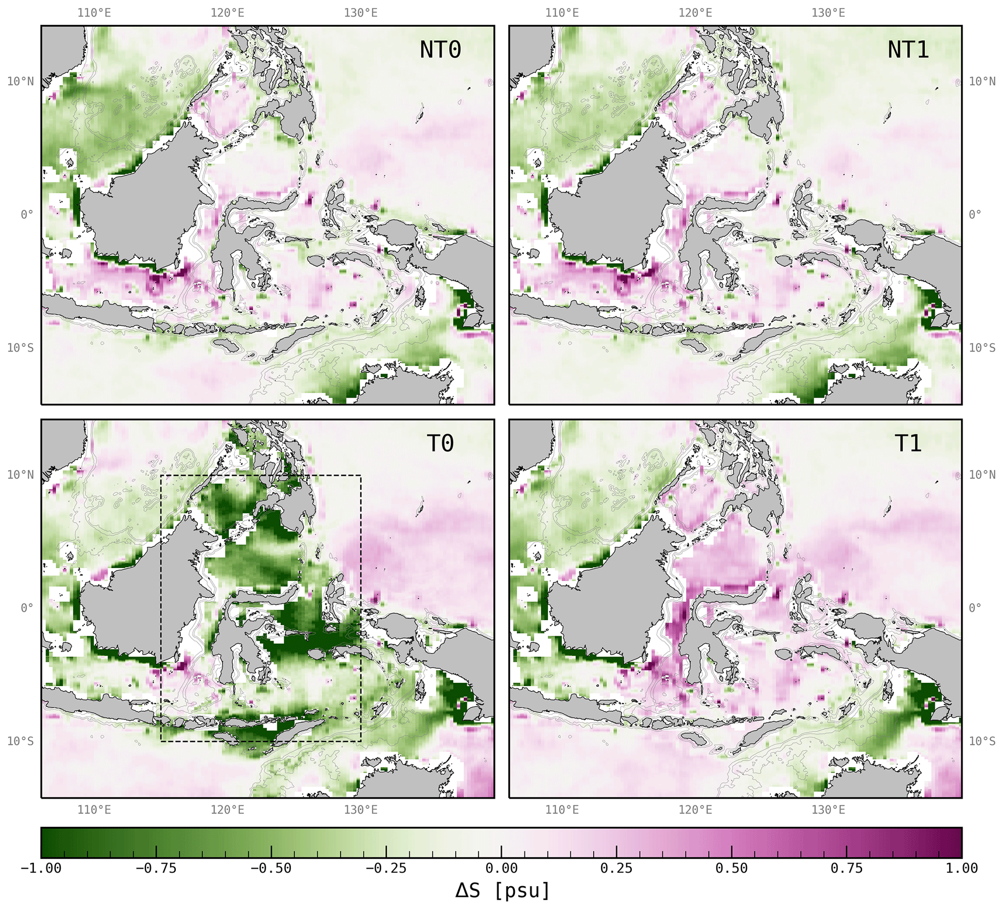
Figure 7 Mean SSS bias with respect to the SMAP/SMOS dataset ($\mathrm{\Delta }\text{S}=\text{SSS(SYMPHONIE)}-\text{SST(SMAP/SMOS)}$) for T0, NT0, T1 and NT1 simulations computed over the years 2017–2018. Positive values correspond to an overestimation in the model output. The 100, 500 and 1000 m isobaths are also displayed (fine grey lines).

Figure 8 Absolute mean latent heat flux (in W m⁻²) computed over the zone defined by the square in Fig. 7 for all the simulations. Error bars correspond to 1 standard deviation computed over monthly averaged values and the same spatial domain.

4 Discussion

Comparisons among a set of four sensitivity simulations, with and without tides and with and without activation of the filtered formulation and with available Argo temperature and salinity profiles and OSTIA sea surface temperature data, showed that the filtered formulation brings numerical diffusion down to a level that allows for a correct representation of water masses in our simulations over the south-east Asian seas even under strong tidal motions. Through a comparison with the highly diffusive QKE scheme in its raw formulation and with simulations without tides, we have highlighted the spurious numerical effect that tides can have, while stressing their physical importance in transforming the water masses. Nevertheless, some questions remain open.

First of all, the choice of the filter in Eq. (12) is still weakly constrained. For the sake of simplicity and to stick to the original formulation proposed in Juricke et al. (2020a), we chose a simple three-point average and achieved satisfying results. We can, however, wonder if another filter could be better suited. Basically, we would like the filter to have its cutoff wavenumber, θ_c, equal to the lowest wavenumber that the advective part of the scheme, 𝒜, can effectively resolve in order to ensure that all the noise is effectively dissipated while the well-represented scales are protected from spurious damping. It is debatable whether such a clear separation between noise and physics can be drawn as it will always rely on the definition of an arbitrary condition (such as in Kent et al., 2014, or Winther et al., 2007). Nonetheless, following computations made by Winther et al. (2007), the minimum wavelength accurately represented by a fourth-order central differencing scheme is approximately N=4.4 grid points. Defining the cutoff wavenumber of a filter in a standard way as the wavenumber θ_c at which $\widehat{\mathit{\varphi }}\left({\mathit{\theta }}_{\mathrm{c}}\right)\approx \mathrm{1}/\sqrt{\mathrm{2}}$ (as is commonly done in signal processing), we have, for ϕ₃, a cutoff wavelength of $N_{\mathrm{c}}=\mathrm{2}\mathit{\pi }/{\mathit{\theta }}_{\mathrm{c}}\approx \mathrm{5.5}$ grid points. That is, the cutoff of our filter is slightly greater than the actual accuracy of the advective part, ensuring that all the noisy wavelengths are effectively filtered out. On the contrary, for a higher-order filter of the form

$$\begin{array}{}\text{(18)}& {\mathit{\varphi }}_{\mathrm{5}*}[s{]}_j=s_i+{\displaystyle \frac{\mathrm{1}}{\mathrm{16}}}(-s_{j+\mathrm{2}}+\mathrm{4}{s}_{j+\mathrm{1}}-\mathrm{6}{s}_j+\mathrm{4}{s}_{j-\mathrm{1}}-s_{j-\mathrm{2}}),\end{array}$$

the transfer function of which is written as

$$\begin{array}{}\text{(19)}& {\widehat{\mathit{\varphi }}}_{\mathrm{5}*}\left[k\right]=\mathrm{1}-{\displaystyle \frac{\mathrm{1}}{\mathrm{4}}}(\mathrm{1}-\cos \mathit{\theta }{)}^{\mathrm{2}},\end{array}$$

with a cutoff wavelength of approximately N_c=3.8 grid points. This is slightly lower than but comparable to the above defined accuracy of 4.4 grid points. Considering the rather approximative aspect of these computations, we could thus still consider this other filter valid. However, the stencil required to compute such a filter is wider than for ϕ₃ (five grid points for ϕ_5* vs. three for ϕ₃), increasing the computational cost and numerical complexity, especially when computing boundary conditions. The ϕ₃ filter is therefore a rather good compromise even though other filters have not been tested in the scope of this study, but we cannot exclude that other, possibly non-linear, filters might be better suited in other situations.

Second, the choice of this filter leads to an interesting result that raises the question of choosing between the UP3-F and UP5 schemes. Looking at Eq. (15), it turns out that except for the multiplying coefficient $\mathrm{1}/\mathrm{6}$, the damping coefficient for the filtered formulation of the UP3 scheme, γ^UP3-F, is equal to the damping coefficient for a fifth-order upwind biased scheme (UP5); namely, the following applies:

$$\begin{array}{}\text{(20)}& {\mathit{\gamma }}^{\text{UP5}}={\displaystyle \frac{\mathrm{8}W}{\mathrm{60}\mathrm{\Delta }z}}(\mathrm{1}-\cos \mathit{\theta }{)}^{\mathrm{3}}.\end{array}$$

See, for instance, Soufflet et al. (2016) for the derivation of γ^UP5. This is also illustrated in Fig. 2. Basically, this means that the diffusive part of our filtered formulation of the UP3 scheme is equivalent to the diffusive part of a UP5 scheme; that is, it is a tri-Laplacian operator. This result is similar to the one described in Juricke et al. (2020a), where the filtered harmonic diffusion boils down to a biharmonic diffusion when α is set to 1. We can therefore wonder if it would not be preferable to directly use a UP5 scheme instead of a filtered scheme since it should overall achieve a higher order of accuracy. The answer is most likely. There are, however, several aspects to be considered here. Though it might be negligible in comparison to the cost of computing other components of the model, the computational cost of the UP5 scheme is slightly higher than the one of the UP3-F formulation since in UP3-F, only the dissipative component uses a larger stencil. However, more importantly, the base scheme actually used in Symphonie is QKE. It should be possible to build a scheme similar to QKE on the UP5, but some additional work would be necessary and has not been carried out as part of the scope of this study. Moreover, we should keep in mind that Eq. (15) is derived from Eq. (14) in the particular case where α=1. Though other values of α have not been discussed here, formulations where α≠1 (and especially α>1) are believed to have some potential in further reducing numerical mixing and will be investigated in further studies. Taking a step back, this result nevertheless suggests that a bi-Laplacian diffusion is still too dissipative, while a tri-Laplacian operator could achieve better results, at least in the situation studied here. This result might be of importance for existing and upcoming numerical cores since increasing the order of the diffusion might be a rather affordable option.

5 Conclusions

In this paper, we have presented a new way of formulating the vertical advection scheme in the Symphonie model that builds on a previously available scheme and aims at making its diffusive component more scale-selective, thus reducing spurious numerical mixing, especially in a context where tides are explicitly resolved. This method has then been validated in a regional model of the south-east Asian seas, which is known to be the generation site of strong internal tides that dissipate in the semi-enclosed basins of the region. By running simulations with and without tides and with the new formulation turned on and off, we have shown that the numerical diffusion is reduced enough so that the model is able to satisfyingly represent observed water masses throughout the various seas and surface fields. At the same time, we provided a clear illustration of the spurious effect that tides can have in a fixed-coordinate model, even in a regional model that is forced at its lateral boundaries. The impact of spurious mixing on the SST is particularly important, considering its non-linear interactions with the atmosphere, as illustrated by the large fresh bias at the surface that is observed in the highly diffusive simulation. The effect can be even worse in fully coupled atmosphere–ocean simulations as the whole atmosphere will adjust to the modified SST, potentially biasing the entire response of the model.

This issue of spurious numerical mixing induced by tides, although previously known, has, to our knowledge, not been reported before as explicitly as in this study. We believe this to be helpful to the growing community of model users who are not necessarily well versed in numerical modelling. We advocate for a better recognition of spurious vertical mixing and its effect, especially in the context of long simulations run with explicit tidal forcing, and of the importance of carefully choosing the proper numerical methods.

Some aspects, however, still remain uncertain and call for further work. The spurious effect of numerical mixing on tracer fields is rather coarse and qualitative. A more thorough quantification might provide, however, valuable insight that can help to further disentangle numerical from physical mixing and assess the relative contribution of each process in the observed results, from surface fields to tracer profiles. The choice of such a method is, however, not straightforward, each exhibiting their own strengths and limitations (see, for instance, Banerjee et al., 2024).

Focusing more specifically on the advection scheme presented in this paper, the choice of the filter to be used is still weakly constrained, thus calling for further investigations. A comparison to other standard schemes, though out of the scope of this paper, could also be carried out. At the same time, owing to the variety of approaches in ocean modelling, the idea of defining a universal advection scheme is still difficult if not delusional. The choice of a method indeed always involves a compromise between the quality of the solution, which is by itself oddly defined and depends on the problem itself; algorithmic complexity, which might prevent the use of a particular method on a particular set of coordinates, for example; and computational cost. This is also the reason why modern dynamical cores usually offer users the possibility of choosing between several advection schemes depending on their needs. As stated in Gerdes et al. (1991), as long as the theoretical basis of a scheme is justified, the realism of the resulting simulation when compared to observations is the only way to define what is “best”. The method presented here should therefore be seen more as a new element in a much wider toolbox of solutions aiming at reducing numerical errors in ocean models rather than a definitive solution to the issue of spurious vertical mixing.

Appendix A: Location and number of Argo floats in the region

Figure A1 shows the distribution of Argo profiles in the region. In the interior basins, all data over the period of interest have been selected. In the eastern Indian Ocean, considering the large amount of data available, only a subset of profiles sampling the exit of the ITF has been selected.

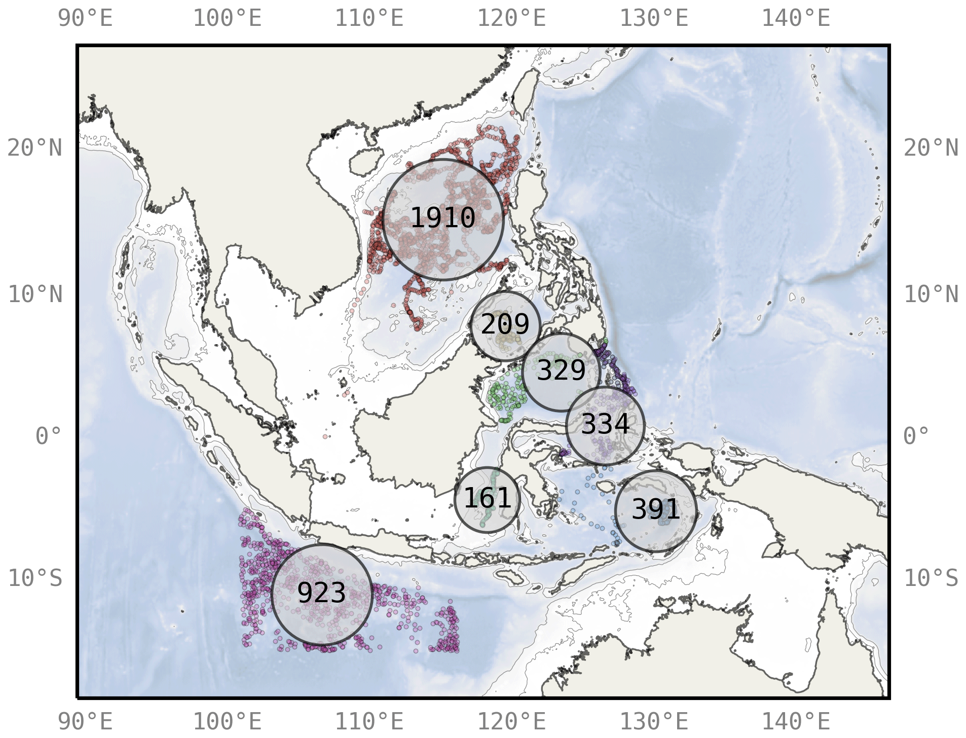
Figure A1 Locations and number of Argo floats in each basin of the region over the 2017–2018 period. Individual profiles are represented by coloured points, while the numbers in large circles indicate the number of profiles in each basin over the period of interest. Basin names are provided in Fig. 1.

Appendix B: Metric for profile comparison

For each zone b and each depth level k, the standard deviation ${\mathit{\sigma }}_k^b$ for the Argo data in the zone is computed. The RMSE is then computed by weighting each depth level k by $w_k^b=(\mathrm{1}/{\mathit{\sigma }}_k^b)/({\sum }_j\mathrm{1}/{\mathit{\sigma }}_j^b$). This modified metric is referred to as weighted RMSE (wRMSE) and is written as follows:

$$\begin{array}{}\text{(B1)}& \text{wRMSE}[X_b^s,X_b^r]=\sqrt{\sum _k{w}_k^b\left(X_b^s\right[k]-X_b^r[k]{)}^{\mathrm{2}}},\end{array}$$

where ($X_b^s\left[k\right]$)_k is a profile sampled at m depth levels which are indicated using the notation k in zone b for a given simulation s and with ($X_b^r\left[k\right]$)_k being a reference profile (e.g. Argo). Choosing weights in this way means that less importance, compared to ordinary RMSE, is given to depth levels where the observed variations quantified by σ_k are greater, and, conversely, more importance is given to levels with less variation between the various profiles.