Implementing the iCORAL (version 1.0) coral reef CaCO₃ production module in the iLOVECLIM climate model

Coral reef development is intricately linked to both climate and the concentration of atmospheric CO₂, specifically through temperature and carbonate chemistry in the upper ocean. In turn, the calcification of corals modifies the concentration of dissolved inorganic carbon (DIC) and total alkalinity in the ocean, impacting air–sea gas exchange, atmospheric CO₂ concentration, and ultimately the climate. This feedback between atmospheric conditions and coral biogeochemistry can only be accounted for with a coupled coral–carbon–climate model. Here we present the implementation of a coral reef calcification module into an Earth system model. Simulated coral reef production of the calcium carbonate mineral aragonite depends on photosynthetically active radiation, nutrient concentrations, salinity, temperature, and the aragonite saturation state. An ensemble of 210 parameter perturbation simulations was performed to identify carbonate production parameter values that optimize the simulated distribution of coral reefs and associated carbonate production. The tuned model simulates the presence of coral reefs and regional-to-global carbonate production values in good agreement with data-based estimates, despite some limitations due to the imperfect simulation of climatic and biogeochemical fields driving the simulation of coral reef development. When used in association with methods accounting for bathymetry changes resulting from different sea levels, the model enables assessment of past and future coral–climate coupling on seasonal to millennial timescales, highlighting how climatic trends and variability may affect reef development and the resulting climate–carbon feedback.

1 Introduction

Tropical coral reefs are well known for the provisional and cultural ecosystem services they provide, supporting large fisheries (Hoegh-Guldberg, 1999) and a multi-billion-dollar tourism industry (Spalding et al., 2017). However, they also play an important role in the carbon cycle and hence climate regulation. The production of calcium carbonate by coral reefs consumes total alkalinity and dissolved inorganic carbon at a ratio of 2:1, decreasing pH, increasing [CO₂], and in an open system resulting in outgassing of CO₂ to the atmosphere (Gattuso et al., 1999; Bates et al., 2001; Wolf-Gladrow et al., 2007; Suzuki and Kawahata, 2003). On the contrary, dissolution of calcium carbonate has the opposite effect, acting to lower the concentration of atmospheric CO₂.

Due to this effect, coral reefs have been proposed as a possible cause of the deglacial CO₂ increase from the cold Last Glacial Maximum around 21 000 years ago to the warmer Holocene around 9000 years ago. During this deglaciation period, the sea level rose by around 120 m (Gowan et al., 2021). It has been hypothesized that this led to the colonization of flooded continental shelves by coral reefs, with enhanced global calcification, with increasing atmospheric CO₂, and acting as a positive feedback on deglacial warming. This hypothesis was first proposed by Berger (1982) and was subsequently tested and discussed in several studies (Opdyke and Walker, 1992; Walker and Opdyke, 1995; Munhoven and Francois, 1996; Kleypas, 1997; Ridgwell et al., 2003; Vecsei and Berger, 2004). Although the scale of coral contribution to the deglacial CO₂ rise is not well constrained, its potentially substantial role in interglacial CO₂ changes, such as those during the Holocene, has been demonstrated (Ridgwell et al., 2003; Kleinen et al., 2016; Menviel and Joos, 2012; Brovkin et al., 2016).

As climate is projected to change in the future, so is the extent and distribution of coral reef cover, which is influenced by sea level, ocean temperature, nutrient concentrations, and carbonate chemistry. Studies of long-term (>1000 years) evolution of the future carbon cycle have mostly focused on the effect of deep-sea sediments (Archer, 2005; Archer et al., 2009), overlooking the potential influence of coral reef changes on tropical shelves.

To understand and evaluate the role of coral reefs in the carbon cycle and their resulting effect on climate, it is necessary to use a carbon–climate model that includes a coral reef carbonate production module. Based on studies investigating the effect of warming and/or ocean acidification on corals (either in situ or in laboratories), empirical models have been developed to evaluate coral reef changes, regionally or globally (Kleypas et al., 1999a; Donner et al., 2005; Buddemeier et al., 2008; Silverman et al., 2009; Pandolfi et al., 2011; Frieler et al., 2013; Couce et al., 2013a, b; Kwiatkowski et al., 2015; van Hooidonk et al., 2016). However, most of these focus on the development and bleaching of corals and not explicitly on carbonate production. In addition, they do not take into account the feedback on the rest of the carbon cycle, which would alter the response. Less than a handful of models of coral reef carbonate production have been developed, and most have shown poor performance compared to observations (Jones et al., 2015). In addition, with the exception of the CLIMBER-2 intermediate-complexity model (Kleinen et al., 2016), no coral reef carbonate production model has been coupled to a climate–carbon model. Instead, simulations with climate models have been limited to prescribing dissolved inorganic carbon (DIC) and alkalinity fluxes associated with net calcification and dissolution (Ridgwell et al., 2003; Kleinen et al., 2010; Brovkin et al., 2019; O'Neill et al., 2021). Moreover, using climate model outputs to force coral niche or impact models offline, as has been the case historically, has limitations. Simulated variables from climate models are not always archived at the needed temporal resolution. While annual and monthly outputs are usually available, daily and diel values are often not kept for simulations of more than a century due to the associated storage requirement. This prevents precise computation of simulated bleaching events using degree heating weeks (DHWs) and/or accounting for sub-monthly carbonate chemistry variability (Torres et al., 2021; Kwiatkowski et al., 2022). Directly coupling a coral reef module to a climate model negates such limitations.

Here we have implemented a coral calcification module into the iLOVECLIM carbon cycle–climate model. iLOVECLIM is an intermediate-complexity model well suited for multi-millennial climate simulations and has already been used in numerous studies addressing changes during the Last Glacial Maximum (Lhardy et al., 2021), past interglacials (Bouttes et al., 2018), and the last 2000 years (Bakker et al., 2022). The coral module described here is based on the ReefHab model (Kleypas, 1995, 1997), but it includes several extensions to improve its performance and account for wider process complexity. Specifically, given that warming and heat waves leading to bleaching can severely impact coral reefs (Sully et al., 2019) and that ocean acidification can hinder calcification (Chan and Connolly, 2013; Albright et al., 2018), we have incorporated a bleaching component and parameterizations of coral reef carbonate production that are dependent on temperature and aragonite saturation state.

While the coral reef model could be best calibrated and compared to observations using present-day environmental conditions, we aim for iLOVECLIM applications to climates far beyond the current state. Therefore, we use a dual approach. We test the model using the best observational drivers but make sure that we could link these drivers to internal model variables or use simplified approaches applicable for a wide range of climates. However, the coupled model application to other climates is beyond the scope of this paper.

2 Methods

We have coupled the iLOVECLIM climate model (version 1.1.6) to a new tropical coral reef module (iCORAL version 1.0). We describe the model, simulations, and data used to select the best parameter sets and validate the new coupled model in modern conditions.

2.1 Description of the iLOVECLIM model (version 1.1.6)

iLOVECLIM (version 1.1.6) is an intermediate-complexity model including atmosphere (ECBILT), ocean (CLIO), sea ice (LIM), and continental vegetation (VECODE) components inherited from the LOVECLIM model (Goosse et al., 2010). The ice sheet module (not used in this version) and the ocean carbon cycle module (used in this version) differ from LOVECLIM (Bouttes et al., 2015). iLOVECLIM has a horizontal ocean resolution of 3° with 20 vertical levels (including 6 levels in the upper 100 m), while the atmosphere is a T21 quasi-geostrophic model with 3 vertical levels. It is well suited to long-duration and large-ensemble simulations as it can simulate around 700 years d⁻¹ on a 7-core CPU.

The ocean carbon cycle, which is the standard carbon cycle module of iLOVECLIM (Bouttes et al., 2015), is based on a Nutrient–Phytoplankton–Zooplankton–Detritus (NPZD) model (HAMOCC3.1; Six and Maier-Reimer, 1996; Brovkin et al., 2002). It includes dissolved inorganic carbon (DIC) and alkalinity (ALK). The air–sea gas exchange of CO₂ depends on sea ice coverage, wind speed, and the air–sea pCO₂ gradient. Surface ocean pCO₂ is computed from temperature, salinity, DIC, and ALK using the polynomial A_CBW solver from SolveSAPHE (Munhoven, 2013), updated to revision 1.0.3 (Munhoven, 2020), with the pH_SWS configuration. The surface oxygen concentration is prescribed to saturation. The model comprises one phytoplankton type, one zooplankton type, nutrients (nitrate and phosphate), oxygen, two types of dissolved organic carbon (labile and refractory), particulate organic carbon (POC), and calcium carbonate in the form of calcite (CaCO₃) that results from implicit pelagic calcification. Photosynthesis is prescribed in the euphotic zone, set as the upper 100 m. All tracers follow the advection–diffusion scheme of the ocean model, with the exception of POC and CaCO₃ which sink and are remineralized at depth with a fixed vertical profile.

2.2 Description of the iCORAL (version 1.0) coral reef module

The coral reef module, called iCORAL (interactive CORAL reef accumulation module) is a module of calcium carbonate (aragonite) production based on the ReefHab model (Kleypas, 1995, 1997) with several modifications and developments that we describe below. It aggregates the carbonate production of warm-water coral reef ecosystems composed of corals, calcareous algae, and other calcifiers depending on local variables.

2.2.1 Coral habitability

As in ReefHab, iCORAL first computes the coral habitability in each grid cell. The habitability is based on modern observations of coral presence and environmental conditions (Kleypas et al., 1999b, and references therein). Coral carbonate production can take place in a grid cell under the requirement that the following conditions are satisfied:

• The temperature is between 18.1 and 31.5 °C and exceeds 18.1 °C throughout the year.

• The salinity is between 30 and 39.

• The phosphate concentration is below 0.2 µmol L⁻¹.

• The depth Z is shallower than the maximum coral production depth (Z_max), which depends on the attenuation of light in the water column,

  $$\begin{array}{}\text{(1)}& Z_{\max }={\displaystyle \frac{\log \left(\frac{I_{\min }}{\text{PAR}}\right)}{K_{\mathrm{490}}}},\end{array}$$

  where I_min is a fixed parameter (the minimum light intensity necessary for reef growth) that is optimized during model tuning (Table 1), PAR is the photosynthetically active radiation at the surface (computed by the iLOVECLIM climate model), and K₄₉₀ is the diffuse attenuation coefficient at 490 nm taken from the Level-3 binned Aqua MODIS products in the OceanColor database (available at http://oceancolor.gsfc.nasa.gov, last access: 19 February 2020). The MODIS data are taken from the entire mission composite at 9 km resolution, encompassing 15 years from 2002 to 2016, and have been regridded on the CLIO grid (3° by 3°). The production depth is defined as the depth at which light is at the I_min level.

The nutrient and salinity thresholds utilized in the coral module are similar to those of ReefHab. The thermal limits, however, use the temperature in each grid cell at each depth, unlike ReefHab, which only uses sea surface temperatures.

2.2.2 Calcium carbonate production

Once coral habitability has been determined, the production of calcium carbonate (P) depends on several local variables. The carbonate production is computed as

$$\begin{array}{}\text{(2)}& \begin{array}{rl}P& =g_{\max }\times f_{\mathrm{R}}\left(\text{PAR}\right)\times f_{\mathrm{T}}\left(T\right)\times f_{\mathrm{O}}\left(\mathrm{\Omega }\right)\\ & \times S_{\mathrm{avail}}\times \mathit{\text{TF}}\times f_{\mathrm{B}}\left(t;t_{\mathrm{bleach}}\right),\end{array}\end{array}$$

where g_max is the maximum value that is a tuning parameter (Table 1), f_R(PAR) is a function of the photosynthetically active radiation at the surface (PAR), f_T(T) is a function of the temperature (T), f_O(Ω) is a function of the aragonite saturation state (Ω), S_avail is the available surface area, TF is the topographic factor, and f_B(t; t_bleach) is a function for the bleaching. This equation expands on that used in ReefHab, which was similar but without f_T(T), f_O(Ω), and f_B(bleach). Because the vertical resolution in the model is relatively coarse (increasing from 10 m at the surface to 28 m at 100 m depth), coral production is computed on a sub-level vertical grid every metre (Fig. S1 in the Supplement). This allows us to account for the fine vertical changes in light attenuation, surface availability, and bathymetry. The other variables, taken from the ocean model, are homogenous in an ocean grid cell (temperature and aragonite saturation state). The carbonate production at 1 m vertical resolution is then aggregated in each ocean cell.

The local variables governing the calcium carbonate production are as follows:

• a.

  Light availability. Calcification is assumed to be directly proportional to photosynthesis (Chalker, 1981). The production is a function of light depending on surface photosynthetically active radiation (PAR) and its attenuation with depth. The function, as for ReefHab, uses a hyperbolic tangent (Jassby and Platt, 1976; Bosscher and Schlager, 1992):

  $$\begin{array}{}\text{(3)}& f_{\mathrm{R}}\left(\text{PAR}\right)=\tanh \left({\displaystyle \frac{I_z}{I_k}}\right),\end{array}$$

  where $I_z=\text{PAR}\times e^{\left(-K_{\mathrm{490}}\times z\right)}$. z is the depth at the sub-grid level (every metre), K₄₉₀ is again the diffuse attenuation coefficient at 490 nm, and I_k is a parameter used in the model tuning (Table 1).

• b.

  Temperature. The study by Jones et al. (2015) showed that the best results for coral production are obtained with a linear relationship between calcification and temperature. We have thus added a linear function of temperature (T), in degrees Celsius, fitted for the temperature range of coral reef habitability (f_T(T)=0 at T=18.1 °C, and f_T(T)=1 at T=31.5 °C; f_T(T)=0 outside the range of 18.1–31.5 °C):

  $$\begin{array}{}\text{(4)}& f\left(T\right)=-\mathrm{1.38}+\mathrm{0.077}\times T.\end{array}$$
• c.

  Aragonite saturation state. Following Langdon and Atkinson (2005), we have added a function depending on the aragonite saturation state (Ω) defined as the ratio of the ion concentration product to the solubility product (K_sp) for the mineral aragonite at the in situ temperature, salinity, and pressure:

  $$\begin{array}{}\text{(5)}& \mathrm{\Omega }={\displaystyle \frac{\left[{\mathrm{Ca}}^{\mathrm{2}+}\right]\left[{\mathrm{CO}}_{\mathrm{3}}^{\mathrm{2}-}\right]}{K_{\mathrm{sp}}}}.\end{array}$$

  The production function is then

  $$\begin{array}{}\text{(6)}& \begin{array}{ll}\text{if }\mathrm{\Omega }>\mathrm{1}& f_{\mathrm{O}}\left(\mathrm{\Omega }\right)=\frac{\mathrm{\Omega }-\mathrm{1}}{K_{\mathrm{omega}}}\\ \text{else }& f_{\mathrm{O}}\left(\mathrm{\Omega }\right)=\mathrm{0},\end{array}\end{array}$$

  where K_omega is a normalization parameter (K_omega=2.86).

• d.

  The available surface area. S_avail is computed in each grid cell from GEBCO 2014 (GEBCO Compilation Group, 2022; https://www.gebco.net/data_and_products/historical_data_sets/, last access: 19 February 2020) with a 1 m sub-grid vertical resolution. For each vertical 1 m depth interval, we sum the areas from GEBCO corresponding to that level that are contained in a CLIO grid cell. Because of the coarse grid of iLOVECLIM, some ocean areas from GEBCO occur on the continental grid, in which case the surface area is added to the nearest ocean grid cell. These cases represent very small areas and have a negligible impact on model results.

• e.

  A topographic factor, TF, is used to account for the effect of topography as in ReefHab. The calculation follows a two-step parameterization:

  • 1.

    A topographic relief for each grid element, denoted α_ij, is derived by summing up the slopes of the lines connecting its midpoint to the midpoints of its eight neighbouring cells:

    $$\begin{array}{}\text{(7)}& {\mathit{\alpha }}_{ij}=\sum _{n_i=i-\mathrm{1}}^{i+\mathrm{1}}\sum _{n_j=j-\mathrm{1}}^{j+\mathrm{1}}{\tan }^{-\mathrm{1}}\left({\displaystyle \frac{Z_{n_i,n_j}-Z_{ij}}{D_{\left(n_i,n_j\right)-\left(i,j\right)}}}\right),\end{array}$$

    where Z_ij is the depth at the (i,j) midpoint [m], Z_ni,nj is the depth at the (n_i,n_j) midpoint [m], and $D_{(ni,nj)-(i,j)}$ is the distance [m] between midpoints (n_i,n_j) and (i,j).

    Furthermore, α_ij is limited to a maximum of 1.7, which appears to be typical of shelf breaks. Atolls would theoretically present a greater relief, but it appears that atolls or reef areas near steeply sloping continental shelves do not accumulate CaCO₃ any faster than shelf-break reefs. It should be noted that the result of tan⁻¹ in the equation above needs to be expressed in degrees in order to reproduce the values of α reported in Fig. 7 in Kleypas (1997).

  • 2.

    A topography factor, TF, is empirically derived from dynamic simulation experiments, focusing on the Great Barrier Reef, where actual Holocene accumulation rates are well documented. The effective accumulation rate G_eff is then defined as

    $$\begin{array}{}\text{(8)}& G_{\mathrm{eff}}=G\times \mathit{\text{TF}}.\end{array}$$

    According to Kleypas (1997), the most realistic reef thicknesses are obtained with

    $$\begin{array}{}\text{(9)}& \mathit{\text{TF}}={\displaystyle \frac{\ln \left(\mathit{\alpha }\times \mathrm{100}\right)}{\mathrm{5}}}.\end{array}$$

    Reefs along outer continental shelves and mid-ocean atolls have TF values close to 1.0, while topographically uniform inner shelves have TF values near 0.05. α values are limited to a minimum value of 0.01 to avoid physically meaningless negative TFs.

• f.

  An inhibition function depending on bleaching, detailed below. The coral carbonate production is computed daily at each sub-grid vertical level, i.e. at every 1 m depth interval, for each ocean grid cell within the coral habitability range.

2.2.3 Bleaching

Expanding on ReefHab, iCORAL additionally includes a bleaching algorithm based on the degree-heating-week method used by NOAA's satellite-based warning system Coral Reef Watch (https://www.coralreefwatch.noaa.gov/product/5km/methodology.php, last access: 14 July 2024).

We first compute the maximum of the climatological monthly mean temperature over 30 years, i.e. the temperature of the hottest month in the climatological monthly means relative to the grid element (maximum of the climatological monthly mean temperature, MMM_clim). This climatological reference period can either be fixed to the first 30 years of a simulation, which corresponds to no bleaching adaptation of corals to changing temperature, or it is continuously updated with a moving 30-year window to account for some coral adaptation to temperature-induced bleaching.

We then compute the degree heating week (DHW), an index that determines bleaching if it exceeds a prescribed threshold. DHW is a measure of the accumulation of hot spots (HSs) above 1 °C, as prolonged periods of excessive heat are the main driver for bleaching. For this we compute the daily hot spot, which is the difference between the daily temperature (T) and the MMM_clim for the month to which day j belongs.

$$\begin{array}{}\text{(10)}& {\text{HS}}_j=T-{\mathrm{MMM}}_{\mathrm{clim}}\end{array}$$

From these daily hot spots, we derive daily excess hot spots, xHS_j, defined by xHS_j=HS_j if HS_j≥1 and xHS_j=0 otherwise.

The DHW value for a day i is then obtained by summing the daily excess hot spot values over 12 weeks (i.e. 84 d).

$$\begin{array}{}\text{(11)}& {\text{DHW}}_i=\sum _{j=i-\mathrm{84}}^i\left({\displaystyle \frac{{\text{xHS}}_j}{\mathrm{7}}}\right)\end{array}$$

The factor of $\mathrm{1}/\mathrm{7}$ is used to convert the final DHW to units of degree Celsius weeks (°C weeks), as coral bleaching usually develops on the timescale of weeks.

If DHW crosses prescribed critical thresholds, it triggers coral bleaching, which then temporarily limits calcium carbonate production: if DHW exceeds 4 °C weeks the bleaching is regarded as moderate; if DHW exceeds 8 °C weeks it is regarded as severe.

If bleaching has taken place, coral reef carbonate production is limited by the bleaching according to

$$\begin{array}{}\text{(12)}& f_{\mathrm{B}}\left(t;t_{\mathrm{bleach}}\right)=\mathrm{1}-e^{-\frac{t-t_{\mathrm{bleach}}}{{\mathit{\tau }}_{\mathrm{bleach}}}},\end{array}$$

where t_bleach denotes the year in which the most recent bleaching event occurred and t stands for the current year. If the bleaching is severe, the time constant τ_bleach (used in the computation of future carbonate production limitation) is set to 20 years. If the bleaching is moderate, several cases are considered:

1. If the coral reef is not currently recovering from a previous bleaching event, the time constant τ_bleach is set to 5 years.

2. If the coral reef is recovering from a previous moderate bleaching and the time since the previous bleaching event is less than 2 years, then the time constant τ_bleach is set to 20 years (as with for severe bleaching).

3. If the coral reef is recovering from a moderate bleaching event and the time since last bleaching is greater than 2 years ago, then τ_bleach is unchanged.

4. If the coral reef is recovering from severe bleaching, τ_bleach is unchanged.

In addition, if the thermal habitability limit (31.5 °C) is exceeded, it is also assumed that severe bleaching has taken place (τ_bleach is 20 years).

If the last bleaching event was sufficiently long ago (4 times the time constant τ_bleach, meaning 20 years for a moderate bleaching event and 80 years after a severe bleaching event), coral carbonate production is regarded as unaffected by bleaching ($f_{\mathrm{B}}\left(t;t_{\mathrm{bleach}}\right)=\mathrm{1})$.

2.2.4 Impact on the carbon cycle

The production of aragonite by coral reefs impacts the carbon cycle by directly modifying the global inventories of DIC [mol kg⁻¹] and ALK [eq kg⁻¹] in the model:

$$\begin{array}{}\text{(13)}& {\displaystyle \frac{\text{dDIC}}{\mathrm{d}t}}=-P\text{(14)}& {\displaystyle \frac{\text{dALK}}{\mathrm{d}t}}=-\mathrm{2}P,\end{array}$$

where P is the global annual carbonate production [mol kg⁻¹].

As there was no riverine input of carbon and alkalinity to the ocean in iLOVECLIM by default, we have added a homogenous input of alkalinity (A_riv) and carbon (C_riv) at the ocean surface to represent river inputs from weathering. We consider a global constant value C_riv=14 Tmol yr⁻¹, assumed to be all in HCO${}_{\mathrm{3}}^{-}$ form, resulting in A_riv=C_riv. This riverine flux is smaller than the actual observed riverine carbon and alkalinity input because it only compensates for the carbonate loss from the ocean by accumulation in coral reefs, which represents only part of the global ocean carbon and alkalinity sinks.

Weathering removes CO₂ from the atmosphere:

$$\begin{array}{}\text{(15)}& {\displaystyle \frac{\mathrm{d}{C}_{\mathrm{A}}}{\mathrm{d}t}}=-\mathrm{0.5}\cdot C_{\mathrm{riv}},\end{array}$$

where C_A is the global atmospheric CO₂ inventory (Pg C).

Note that the dissolution of coral reef carbonates is not yet explicitly included but will be added in future developments. In addition, we do not consider organic carbon production but only consider carbonate production.

2.2.5 Temperature variability in iLOVECLIM

Due to its simplified atmospheric module, the temperature variability of iLOVECLIM is relatively low compared to observations (Sriver et al., 2014). Unaccounted for, this would bias the simulation of bleaching events using the degree-heating-weeks method. We have thus generated additional temperature variability based upon the analysis of the daily sea surface temperature anomalies in a tropical region with extended coral reef cover (19–16° S, 148–154° E). We fitted a series of autoregressive models of order p, denoted AR(p) models (p=1, …, 6), to the daily time series in each grid point in this area. An AR(p) model predicts the value of a variable at time t as a linear combination of the p previous values plus random noise. The fitting procedure provides the parameter constants for the linear combination (autocorrelation parameters – for details about the dataset used and the processing steps, please see the “Autoregressive Model to Parameterize Temperature Variability” memo in AC4; Bouttes, 2024). Here, we selected the AR(1) model, as the root-mean-square errors (RMSEs) of the higher-order models were not statistically different. Accordingly, we generate an AR(1) variate with an auto-correlation parameter of 0.90 and a Gaussian-distributed random noise with a standard deviation of 0.28 to add daily variability to the otherwise anomalously smooth temperature evolution in iLOVECLIM.

2.3 Simulations

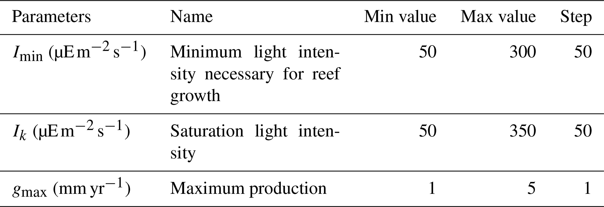
We ran an ensemble of simulations under pre-industrial boundary conditions (atmospheric CO₂ of 284 ppm) with varying values for coral parameters to select the best parameter set compared to existing observational data. To this end, 210 simulations were performed, starting from an equilibrium pre-industrial simulation (Bouttes et al., 2015). Since the 2015 version of iLOVECLIM, the pH calculation routine has been replaced by the SolveSAPHE module based upon the A_CBW approximation to total alkalinity (Munhoven, 2013, 2020). The ensemble of simulations was run with different values for the maximum production parameter g_max, the saturating light intensity I_k, and the minimum light intensity necessary for reef growth I_min (Table 1). In these simulations, there was no feedback from the simulated coral reefs to the climate.

Table 1 Parameter values used in model tuning resulting in an ensemble of 210 simulations. The minimum, maximum, and incremental steps in parameter values used during model tuning are indicated.

2.4 Data used to constrain the model

To constrain the pre-industrial model results, we used published observations of coral reef locations (UNEP-WCMC, 2018; Fig. 1) and global area along with global and regional carbonate production estimates (Perry et al., 2018). Data were mainly for the modern era rather than the pre-industrial. However, a pre-industrial simulation was required in order to initialize historical and future simulations. It was therefore assumed that global coral reef distribution and carbonate production have exhibited limited change over the industrial era. The global area and carbonate production of tropical coral reefs are difficult to evaluate and constrain. According to Vecsei (2004), the total global area ranges between 303 and 345×10³ km², and the global carbonate production ranges between 0.65 and 0.83 Pg CaCO₃ yr⁻¹. More recent global area estimates indicate a range of 284×10³ km² (Spalding et al., 2001) or 150–300×10³ km² (Li et al., 2020). On the other hand, older studies suggested larger values ranging from 600 to 1500×10³ km² (Smith, 1978; Crossland et al., 1991; Copper, 1994). Given this uncertainty and the fact that more recent studies suggest that the largest estimations are probably overestimated, we consider a potential range of 150–600×10³ km².

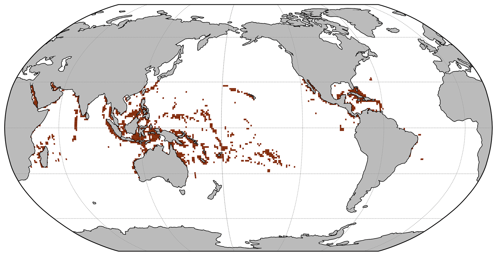
Figure 1 Coral location from the UNEP-WCMC (2018) dataset. Brown cells indicate the presence of coral reefs in these cells. In white grid cells, no coral reefs have been detected.

3 Results

We first evaluate the variables simulated by iLOVECLIM that are relevant for coral production and then compare the coral module results of the ensemble simulations to existing observations of coral reef distribution, area, and carbonate production.

3.1 iLOVECLIM variables

As described in Methods, the main variables simulated by the model that are used to compute coral reef habitability and production are temperature, salinity, phosphate concentration, and aragonite saturation state (Ω) (Fig. 2).

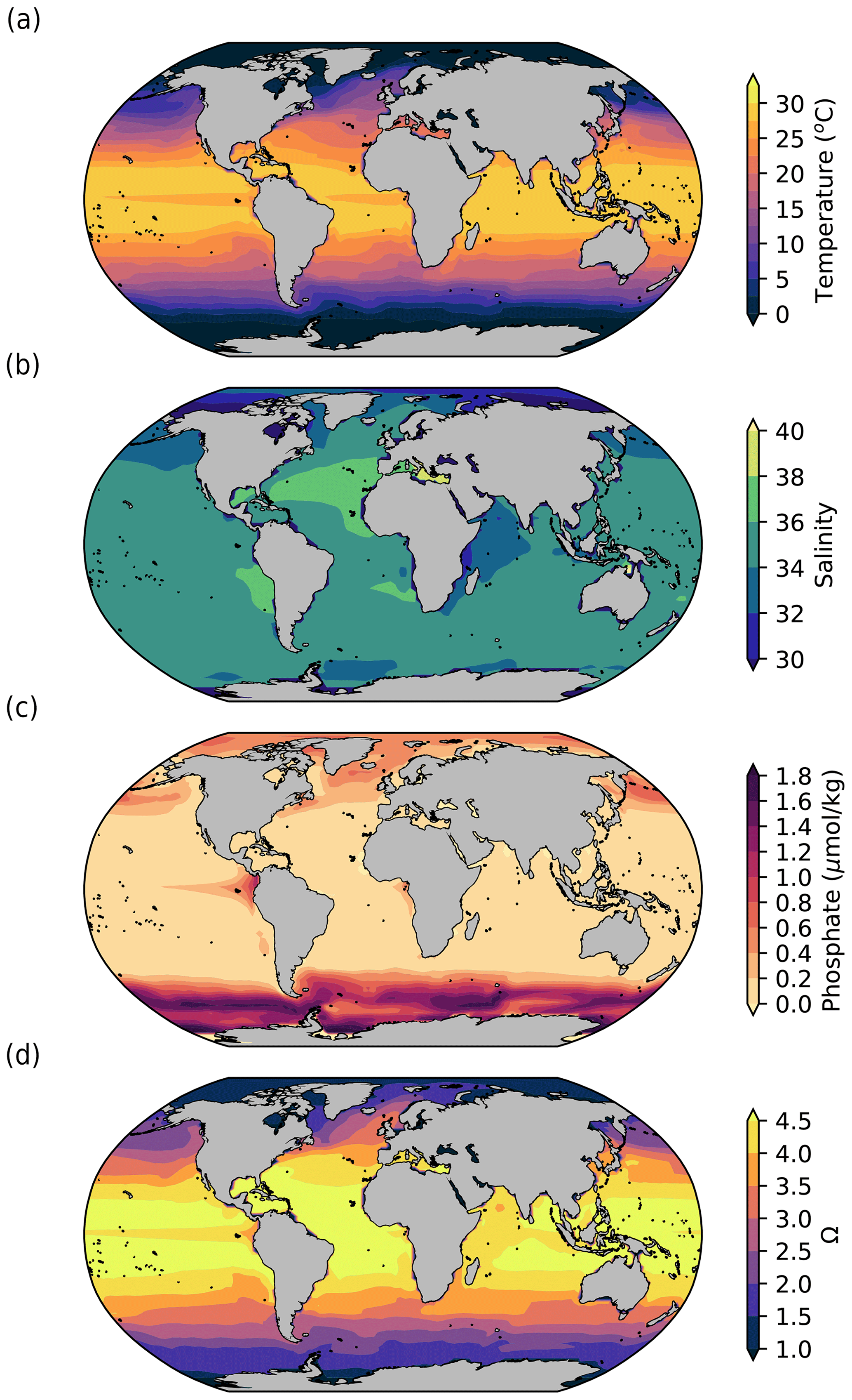
Figure 2 Surface (5 m depth) ocean (a) temperature (°C), (b) salinity, (c) phosphate concentration (µmol kg⁻¹), and (d) aragonite saturation state (Ω) simulated by iLOVECLIM in pre-industrial conditions. The model outputs are 100-year averages at the end of the equilibrium pre-industrial simulation.

In order to compare the iLOVECLIM variables used for coral reef calcification to modern data, we also consider a historical run following the CMIP protocol (Meinshausen et al., 2020) and average the variables over 2000–2010 (Fig. 3). As already evaluated in other studies, iLOVECLIM-simulated sea surface temperature and salinity are in general agreement with data (Goosse et al., 2010; Bouttes et al., 2015), albeit with some regional differences, due partly to the relatively coarse resolution of the model (3° horizontally). The sea surface temperature in the model is generally slightly higher than in the observations, especially in the tropics, where it can be 2 °C higher than in the observations. The coral reef development is limited by a maximum temperature, which could be reached quicker than in observations due to the high temperature bias. The distribution of simulated nutrients exhibits greater biases. The concentrations simulated by the model are generally low compared to observations, especially in eastern equatorial upwelling regions. The resulting effect is the opposite to the one due to the temperature bias: the coral reef development will be less affected by phosphate changes as the maximum limit is further away due to the lower phosphate bias. The saturation state is also in generally good agreement with data, despite some differences locally. In particular, it is slightly higher than the observed values in the tropics.

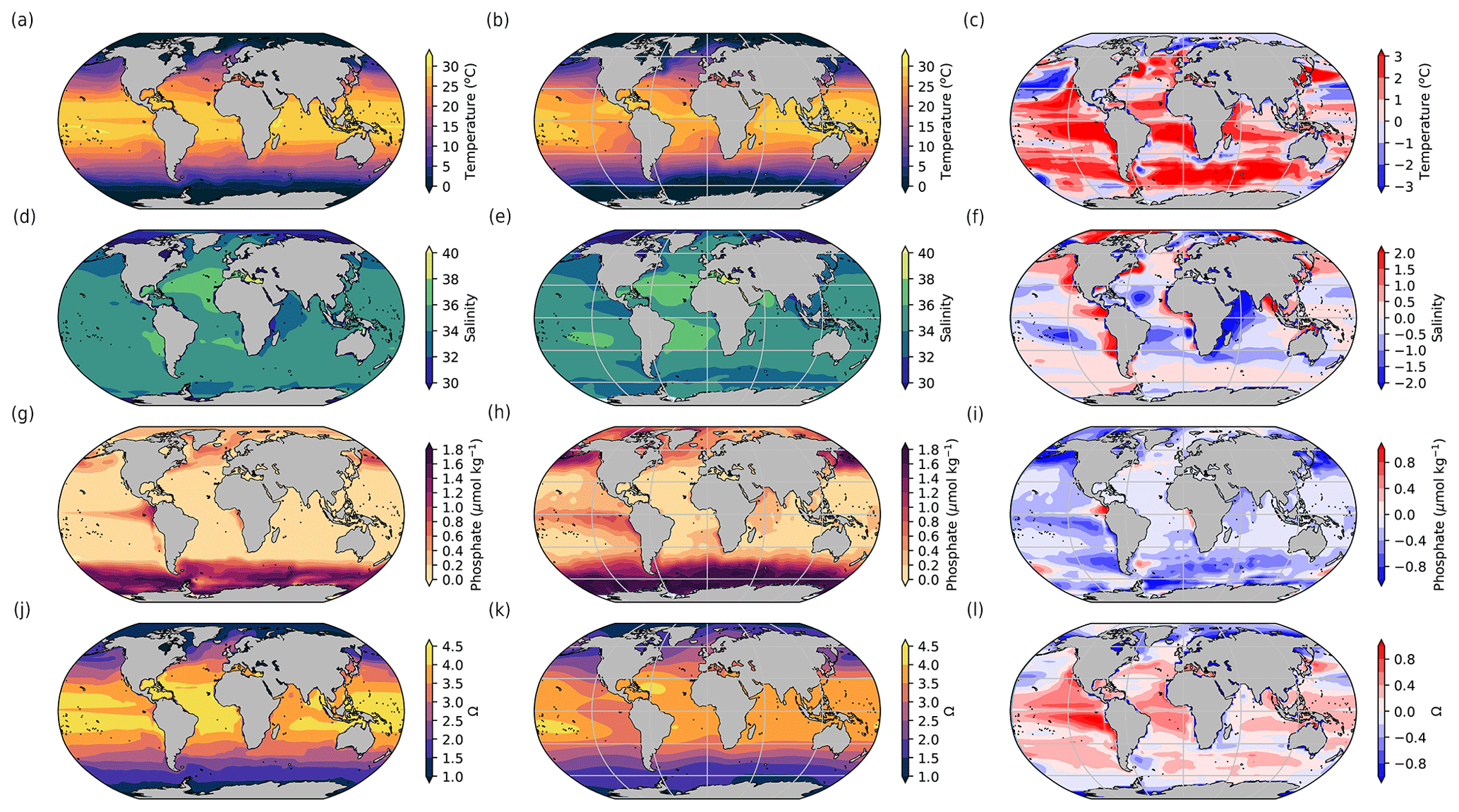
Figure 3 Model (left), observational data (middle), and model–data difference (right) surface maps of (a, b, c) temperature (°C), (d, e, f) salinity, (g, h, i) phosphate (µmol kg⁻¹), and (j, k, l) aragonite saturation state (Ω). The model outputs are averaged over 2000–2010. The data are from Locarnini et al. (2018), Zweng et al. (2018), Garcia et al. (2018), and Jiang et al. (2015). The model outputs are regridded on the data grid to compute the anomaly. The surface in the model corresponds to a grid cell centred at 5 m depth.

3.2 Location and global reef area

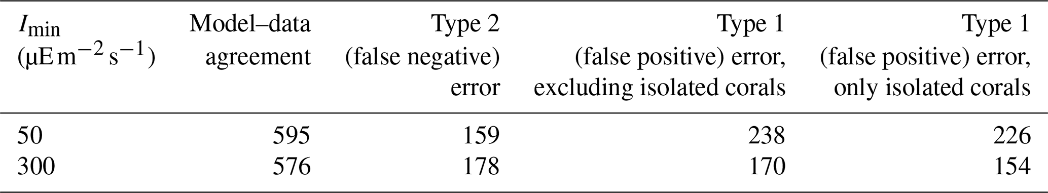
The location of simulated tropical reefs is globally in broad agreement with observational data (Fig. 4). The model computes the presence of corals in most locations where coral reefs have been observed (in blue). However, the model tends to overpredict coral development, i.e. simulates corals in regions where they are not observed, notably in the Atlantic Basin (in beige and purple). Furthermore, it fails to simulate some coral locations observed in the data (in brown), but this mismatch is less widespread. The model could predict coral presence in places where it has not yet been observed, but the overprediction might also be due to the lack of rivers in the model. Indeed, high nutrient concentrations typically prevent coral reef development due to competition with macroalgae, and, in coastal regions, high nutrient concentrations can be partly due to riverine inputs, which are not represented in the model. This could explain some of the mismatch west of Africa. In addition, the model also simulated small isolated coral reefs with small areas (in purple) that might not be captured in the observed data. Alternatively, other limiting factors, not represented in iCORAL, might prevent coral reefs developing in such areas.

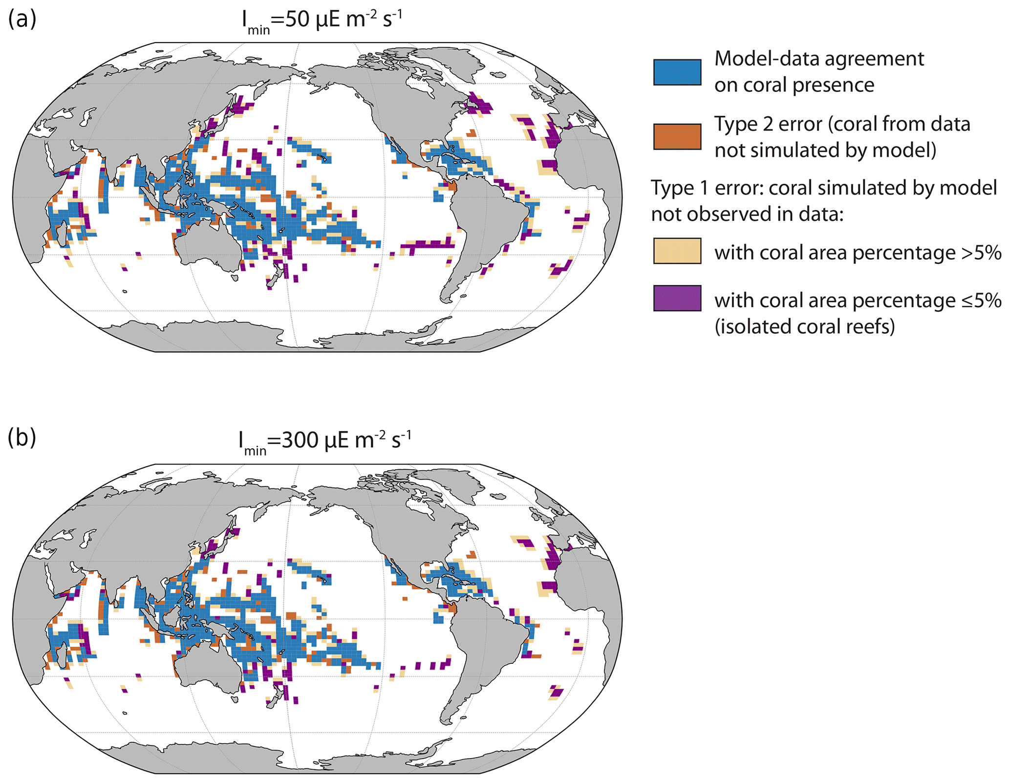
Figure 4 Coral location in the model and data for the minimum and maximum I_min (the minimum light intensity necessary for reef growth) values. Blue cells indicate the presence of corals in both model and observational data, brown cells indicate the presence of corals in observational data but not in the model simulation, and beige and purple cells indicate the presence of corals in the model simulation but not in observations. Some locations correspond to places with very small surface areas (purple, due to small islands, for example), but, as we plot the presence of corals in the relatively large oceanic grid cells (the horizontal ocean resolution is 3° × 3°), it might give the impression of large coral coverage.

Table 2 Number of model grid points with model–data agreement or disagreement. The isolated coral reefs are defined when the coral area ≤5 % of the total area between 0 and −50 m (last column).

The global coral reef area depends on the simulated habitability, which is set by local environmental variables computed by the model, i.e. temperature, salinity, and nutrients, which are identical across our simulations as they are independent of coral carbonate production. It also depends on light availability and on attenuation with depth. The minimum light intensity needed for coral growth is set by the I_min parameter that is changed in our simulation ensemble. Hence I_min is the only parameter among the varied parameters and functions that impacts the simulated reef area.

As I_min increases, the critical depth down to which sufficient light penetrates becomes shallower, and, as a result, the global area covered by coral reefs decreases. The total area ranges from 1500×10³ km² with I_min=50 $\mathrm{\mu }\mathrm{E}{\mathrm{m}}^{-\mathrm{2}}{\mathrm{s}}^{-\mathrm{1}}$ to 390×10³ km² with I_min=300 $\mathrm{\mu }\mathrm{E}{\mathrm{m}}^{-\mathrm{2}}{\mathrm{s}}^{-\mathrm{1}}$ (Table 2). This is less than in Kleypas (1997) for the same I_min parameter values and in better agreement with observational data, but it is still high compared to the observed range of 150–600×10³ km² (Vecsei, 2004; Li et al., 2020) for most simulations. The low-range total areas are nonetheless in agreement with three other model estimations computed by Jones et al. (2015) with the KAG (492×10³ km²), LOUGH (567×10³ km²), and SILCCE (500×10³ km²) models. The total coral reef area is very uncertain, and there are possibilities of both underestimation by data and overprediction by the model.

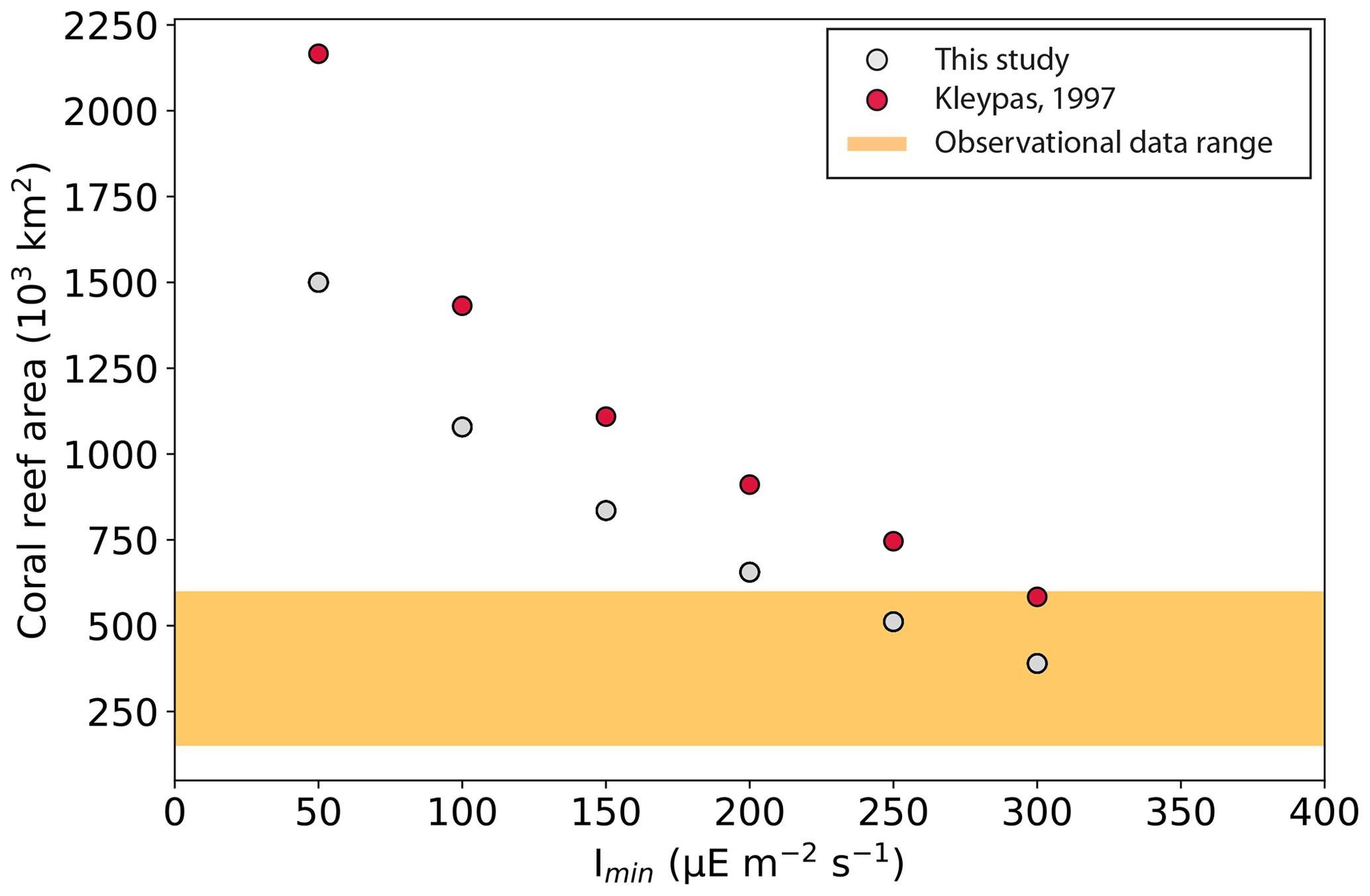
Figure 5 Global coral reef area (10³ km²) simulated in this study and in Kleypas (1997) as a function of I_min (the minimum light intensity necessary for reef growth, $\mathrm{\mu }\mathrm{E}{\mathrm{m}}^{-\mathrm{2}}{\mathrm{s}}^{-\mathrm{1}}$). The range of observational data for the global coral reef area (Sect. 2.4) is shown with the yellow bar.

3.3 Global and regional calcium carbonate production

According to observation-based estimates, global coral reef carbonate production is between 0.65 and 0.83 Pg CaCO₃ yr⁻¹ (Vecsei, 2004). In our ensemble of simulations, global carbonate production ranges from 0.27 to 8.84 Pg CaCO₃ yr⁻¹. Simulations with global production within the observational range can be found for all I_min and I_k values but only for g_max from 1 to 3 mm yr⁻¹ (Fig. 6). The largest global production is obtained for the lowest I_min and I_k values of 50 $\mathrm{\mu }\mathrm{E}{\mathrm{m}}^{-\mathrm{2}}{\mathrm{s}}^{-\mathrm{1}}$, when the light limitation is less stringent. The largest production is also obtained for the largest g_max (maximum production parameter) value of 5 mm d⁻¹. Contrary to this, low production is obtained with high I_min and I_k and with low g_max.

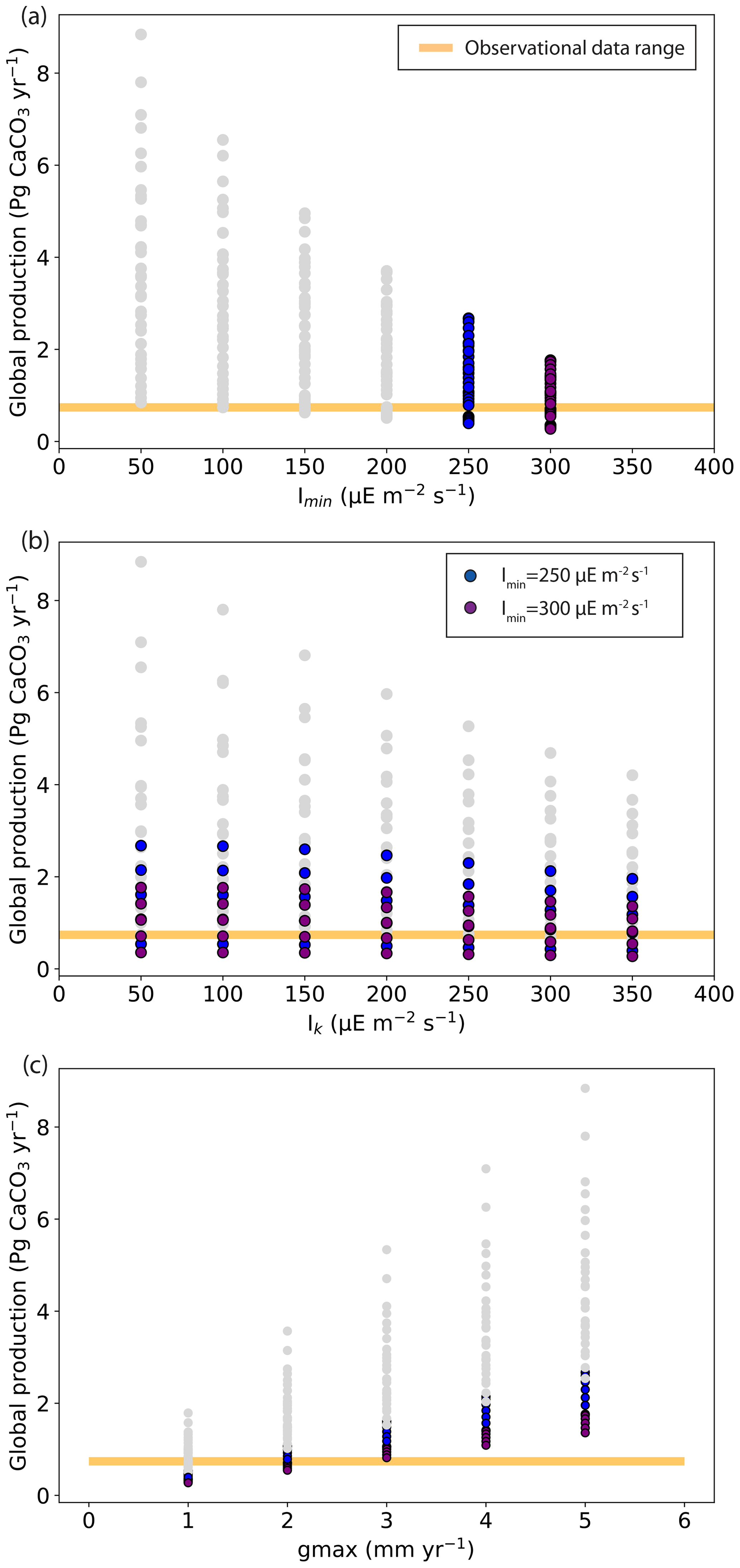
Figure 6 Global coral reef carbonate production (Pg CaCO₃ yr⁻¹) as a function of (a) I_min (the minimum light intensity necessary for reef growth, $\mathrm{\mu }\mathrm{E}{\mathrm{m}}^{-\mathrm{2}}{\mathrm{s}}^{-\mathrm{1}}$), (b) I_k (the saturating light intensity, $\mathrm{\mu }\mathrm{E}{\mathrm{m}}^{-\mathrm{2}}{\mathrm{s}}^{-\mathrm{1}}$), and (c) g_max (the maximum production growth). The range of observational data for the global carbonate production (Vecsei, 2004) is shown with the yellow bar.

When considering model performance with regard to both global reef area and global carbonate production, only six simulations display values in the range of observation-based estimates (Fig. 7 and Table 3). The main limitation comes from the coral reef area, as most of the simulations overestimate coral reef area, with only a handful located within the observed values (Fig. 5).

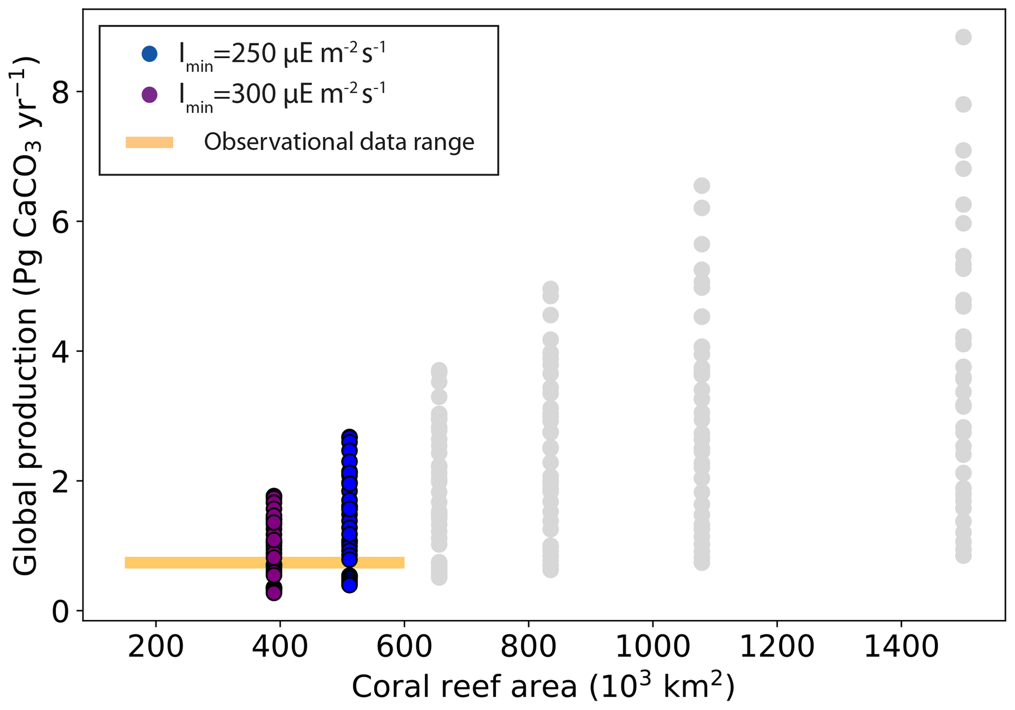
Figure 7 Global carbonate production (Pg CaCO₃ yr⁻¹) as a function of global coral reef area (10³ km²).

Table 3 Global carbonate production, tuning parameters, and root-mean-square error relative to regional production data (Perry et al., 2018) for the simulations with both global production and total area within observational constraints.

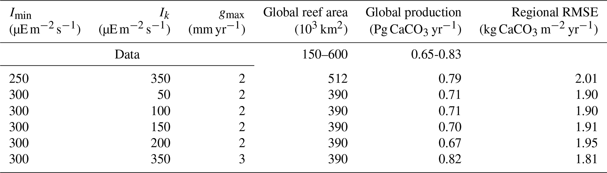
We finally compare model results with the regional carbonate production data from Perry et al. (2018). Figure 8 shows the root-mean-square error (RMSE) between model results and observational data for regional carbonate productivity as a function of global production or global coral reef area. Depending on the parameter choices (Table 3), the model–data agreement varies greatly. The simulations in agreement with both global production and coral reef data are also among those with the lowest RMSE relative to regional production (Table 3), ranging from 1.81 to 2.01 kg CaCO₃ m⁻² yr⁻¹, and are hence in better agreement with all observed data.

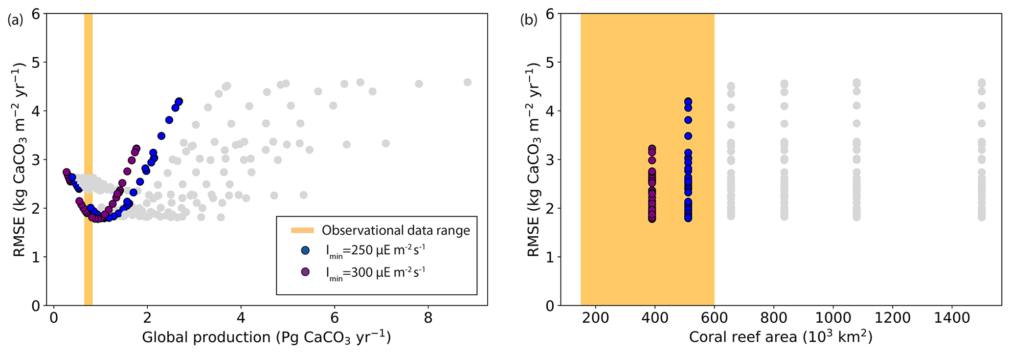
Figure 8 Root-mean-square error (RMSE; kg CaCO₃ m⁻² yr⁻¹) between the simulations and the observational data of regional production (Perry et al., 2018) as a function of (a) global production (Pg CaCO₃ yr⁻¹) and (b) coral reef area (10³ km²).

The six best-performing ensemble simulations when considering both regional and global observational constraints are given in Table 3. All these ensemble members simulate global production within the range of data-based estimates. In these simulations, we have selected the ensemble member with the lowest RMSE (hence the closest agreement with regional production data). Our optimal parameter choices are therefore I_min=300 $\mathrm{\mu }\mathrm{E}{\mathrm{m}}^{-\mathrm{2}}{\mathrm{s}}^{-\mathrm{1}}$, I_k=350 $\mathrm{\mu }\mathrm{E}{\mathrm{m}}^{-\mathrm{2}}{\mathrm{s}}^{-\mathrm{1}}$, and g_max=3 mm yr⁻¹. For this simulation, the global carbonate production is 0.82 Pg CaCO₃ yr⁻¹ and the global coral reef area is 390×10³ km².

4 Discussion

We have presented a new module to compute coral reef production and integrated this module in the iLOVECLIM carbon–climate model. Contrary to Jones et al. (2015), where the coral reef modules were forced by climatic data, we have embedded our module in the coupled carbon–climate iLOVECLIM model. While this will be particularly useful to evaluate coral–climate carbon cycle feedbacks and the response of corals to climate change, it also follows that the module performance will be influenced by the model biases.

4.1 Model caveats

The first limitation is due to the model resolution. The ocean component of iLOVECLIM is a full GCM with 3° horizontal resolution and 20 vertical levels. Hence, local-scale changes in temperature, saturation state, and light penetration below 3° cannot be accounted for in our model. Future work should therefore evaluate the performance of the coral module within higher-resolution ocean components. The vertical-resolution limitation is partly resolved through the use of a sub-grid vertical scale of 1 m to account for light attenuation, but temperature and aragonite saturation state are uniform in each grid box, for which a higher-resolution model would also be useful.

In addition, the simulated nutrient distribution of iLOVECLIM is locally different from observational data. In particular, there are no riverine inputs in iLOVECLIM, resulting in a lack of enhanced nutrient concentrations near river mouths, which can influence coral habitability. This could be more closely looked at in models including rivers input. Finally, light attenuation in the model is currently prescribed based on satellite data. Ideally, however, it would take into account simulated phytoplankton biomass and be computed using marine productivity. As iLOVECLIM has a low resolution and includes a simple NPZD model, computing the attenuation would likely add biases to the model results for the present-day climate. It should nonetheless be tested in future studies, particularly if the module was included in a higher-resolution ocean model and for use in different climates and land configurations. This will be tested in future work.

4.2 Future developments

Besides the climate model, other limitations come from the coral reef module itself. In terms of coral representation, we have only one type of coral representing all communities. However, different communities (or species) respond differently to the driving variables, such as temperature (Coles and Brown, 2003; D'angelo et al., 2015) and aragonite saturation state (Chan and Connolly, 2013; Kroeker et al., 2010, 2013). Further development could thus include several communities with different parameters for their temperature and omega function, similarly to what is done for plankton and zooplankton or for plant functional types (PFTs) on land.

Adaptation to temperature changes is currently an option in the module. The computation of the maximum of the climatological monthly mean temperature (MMM_clim) can either be set to the first 30 years of the simulation (no adaptation) or be set to a rolling mean over a 30-year window evolving in time (adaptation). While adaptation is potentially crucial for coral reefs (Logan et al., 2021), its quantification is poorly constrained and would require more work. In addition to some form of adaptation to bleaching, adaptation of the thermal habitability range could also be taken into consideration. If different coral communities are considered in the future, adaptation could also depend on the coral community.

Dissolution is not yet included, as no existing modern data would allow us to validate this part of the module, but future work considering coral reefs in the past will implement it and use past coral evolution to validate this new addition.

Some processes, such as erosion and bioerosion (Schönberg et al., 2017), are also not currently considered, as they are likely to be of second order or are insufficiently constrained to be included at this stage. In the future, as more knowledge is gathered, they might be worth adding to the module.

In addition, while it is not directly part of the carbonate production module, the use of the coral reef module during past periods (and in long-term future simulations) will require the different bathymetry resulting from sea-level change and the dependency of coral carbonate production on the rate of sea-level change. This should be the topic of future work. Regarding the bathymetry, this can be done following different methods. Some models have implemented schemes to account for bathymetry changes using reconstructions (Meccia and Mikolajewicz, 2018; Bouttes et al., 2023c) that can be used to update the bathymetry regularly. Alternatively, the modern bathymetry can be kept and the sea level can be modified for the considered time period according to proxy data (e.g. Lambeck et al., 2014; Spratt and Lisiecki, 2016). Regarding the carbonate production linked to the rate of sea level change, it can be accounted for by implementing a parameterization (Munhoven and François, 1996; Kleinen et al., 2016).

4.3 Observational constraints on model development

Finally, the model representation highly depends on the functions of environmental variables. The only way to improve this part is through more constraints from in situ and laboratory experiments yielding more information on the functions and parameters used in the model. This modelling approach will thus benefit from all future studies focusing on the response of coral reefs to the values of environmental variables, such as temperature or the saturation state.

5 Conclusions

In conclusion, we have developed a new module, called iCORAL, of coral reef aragonite calcification based on ReefHab (Kleypas, 1995, 1997) for usage in Earth system models. The new developments account for the role of temperature and the saturation state with respect to aragonite in the carbonate production rate. Furthermore, we have added a simple bleaching scheme based upon the successful NOAA Coral Reef Watch rationale. iCORAL has been implemented in the climate–carbon model of intermediate complexity, iLOVECLIM. The simulations with iCORAL–iLOVECLIM are in fair agreement with data in terms of total productivity, areal distribution, and regional productivity. iCORAL–iLOVECLIM is ready to use in studies of coral reef changes in future and past periods, when the role and feedbacks of shelf carbonate accumulation rate changes in the carbon cycle (and hence in climate) need to be evaluated.