New explicit formulae for the settling speed of prolate spheroids in the atmosphere: theoretical background and implementation in AerSett v2.0.2

We propose two explicit expressions to calculate the settling speed of solid atmospheric particles with prolate spheroidal shapes under the hypothesis of horizontal and vertical orientation. The first formulation is based on theoretical arguments only. The second method, valid for particles with mass median diameter up to 1000 µm, is based on recent heuristic drag expressions based on numeric simulations. We show that these two formulations show equivalent results within 2 % for d_eq≤100 µm and within 10 % for particles with d_eq≤500 µm falling with a horizontal orientation, showing that the first, more simple, method is suitable for virtually all atmospheric aerosols, provided their shape can be adequately described as a prolate spheroid. Finally, in order to facilitate the use of our results in chemistry transport models, we provide an implementation of the first of these methods in AerSett v2.0.2, a module written in Fortran.

1 Introduction

Mineral dust plays an important role in the Earth's atmosphere, and in the Earth System overall, influencing radiation, precipitation and biochemical processes. The impact of dust on each of these processes depends strongly on its particle size distribution (PSD). In terms of radiation, fine dust particles (with sizes less than 5 µm) scatter the solar radiation, leading to a cooling effect on the global climate, while coarse particles (sizes larger than 5 µm) tend to absorb both solar and thermal radiation, leading to global warming (Kok et al., 2017). Regarding the precipitation process, dust particles interact with liquid or ice clouds by acting as nucleating particles (Creamean et al., 2013; DeMott et al., 2003; Marinou et al., 2019; Solomos et al., 2011; Twohy et al., 2009). In principle, larger particles are more efficient condensation nuclei, but the number of particles is also an important parameter, and thus the number of particles above a critical size is the quantity that regulates the process (Dusek et al., 2006). Finally, the amount of deposited mass on ocean and land, regulated by the large particles, can stimulate biochemical activity (Jickells et al., 2005).

The PSD vary greatly over space and time after its emission, since the size-dependent process of the gravitational settling removes large particles faster than small particles (e.g., Seinfeld and Pandis, 2006). There is still a large discrepancy between observations and results produced by transport models regarding the evolution of dust particle lifecycle. Although several observation studies have shown that particles with sizes larger than 30 µm can be transported in the atmosphere for days, covering a distance of several thousand kilometers (Goudie and Middleton, 2001; Denjean et al., 2016; Weinzierl et al., 2017; van der Does et al., 2018), several comparisons between model simulations and measurements show that models overestimate the large-particle removal (e.g., Ginoux et al., 2001; Colarco et al., 2002). As a matter of fact, the mass of coarse particles in the atmosphere is estimated to be 4 times larger than the simulated by climate models (Adebiyi and Kok, 2020). All these factors showcase the importance of proper modeling of mineral dust transport.

The most important force that appears in the dynamics of dust particles, significantly modifying their settling velocity, is the drag force. The majority of dust transport models use the Stokes (1851) formulation for the quantification of the drag force (or equivalently the drag coefficient), since they represent mainly spherical particles that are smaller than 20 µm (Kok et al., 2021). For larger particles, a correction must be applied to take into account the deviation from the creeping flow, but all of the corrections are based on empirical data and can lead to significant differences in the calculated settling velocity (Goossens, 2019; Adebiyi et al., 2023). According to a benchmark between different drag coefficient parameterizations suitable for spherical particles of all natural aerosol and particle sizes presented by Goossens (2019), it has been found that the empirical drag coefficient derived by Clift and Gauvin (1971) seems to perform better than all the others.

Drakaki et al. (2022) used the drag coefficient expression of Clift and Gauvin (1971) in the GOCART–AFWA dust scheme of WRFV4.2.1 and managed to increase the simulated size of dust particles from 20 to 100 µm. In the case of coarse and super-coarse particles where the Stoke's approximation is no longer valid, the steady-state equation of motion that has to be solved for the determination of the settling velocity is no longer linear, and numerical methods have to be used instead. Drakaki et al. (2022) used a computationally expensive bisection method. Nevertheless, the inclusion of particles beyond the Stoke's approximation revealed that a reduction in settling velocity of around 60 %–80 % is required for their simulation results to agree with airborne and spaceborne measurements.

Mailler et al. (2023c) improved this computational inefficiency by providing a semi-analytical solution to the drag equation based on the Clift and Gauvin (1971) drag coefficient, eliminating the need for the numerical iterations required by the numerical solution of this nonlinear equation and keeping the numerical error compared to Clift and Gauvin (1971) below 2 %. Their method improved the computational speed by a factor of around 4. The formalism of Mailler et al. (2023c) based on the Clift and Gauvin (1971) drag coefficient is therefore a fast and accurate computational scheme for the study of the settling velocity of spherical particles of all sizes. This formulation has been implemented by the same authors in AerSett v1.0 (Mailler et al., 2023b). AerSett v1.0 is a Fortran module designed for inclusion in chemistry transport models. This module has already been included in Chimere v2023r1 (Menut et al., 2023).

The goal of the current work is to expand this formulation to the case of nonspherical solid particles, focusing on prolate spheroids. As in Mailler et al. (2023c), the point of this study is to obtain an explicit and computationally efficient method for the calculation of the settling speed as a function of known properties of the flow and of the particle. This problem is reciprocal in relation to the classical problem in fluid mechanics (calculating the force as a function of the speed). In atmospheric science, the characteristics of the particle, including the gravity force it is submitted to, are known, while the settling speed is not known a priori, making this classical approach impractical for our problem.

To obtain such an explicit expression of the speed as a function of the other parameters, the first point that has to be addressed is the choice of an accurate expression for the drag coefficient in the case of prolate spheroids. In the Stokes regime, exact analytical solutions similar to the Stokes law for spherical particles (Stokes, 1851) give the values of the drag coefficients in the case of vertically and horizontally oriented prolate spheroids (e.g., Oberbeck, 1876; Jeffery and Filon, 1922; Chwang and Wu, 1975) that can be easily generalized for an arbitrary orientation angle. Additionally, there are higher-order expansions that further increase the accuracy of the calculated drag force (Breach, 1961; Chwang and Wu, 1976).

Many efforts have been made in the past toward the correction of the drag coefficient expressions for larger particles beyond the Stokes regime using different methodologies. In previously published literature there are expressions that have been derived using empirical data (e.g., Bagheri and Bonadonna, 2016, 2019; Dioguardi et al., 2018, and references therein), using computational fluid dynamics (CFD) simulations (e.g., Zastawny et al., 2012; Fröhlich et al., 2020; Sanjeevi et al., 2022, and references therein), or based on theoretical and semi-analytical approximations (e.g., Chwang and Wu, 1976; Mallios et al., 2020, and references therein). It is noted that the correlations derived by empirical data mainly assume a random orientation of the particles, while the correlations based on CFD simulations and the semi-analytical approximations take into account the modification of the drag coefficient expression based on the orientation angle of the particle. Indications of the preferential orientation of settling prolate spheroids has been established in both theoretical and observational basis (e.g., Klett, 1995; Ulanowski et al., 2007; Mallios et al., 2021).

The choice of an appropriate drag coefficient expression is important because it can alter the physical results. Ginoux (2003), using a drag coefficient expression by Boothroyd (1971), showed that the terminal velocities of randomly oriented prolate spheroids and of spheres with the same cross section are practically the same as long as the aspect ratio of the spheroids is less than 5. On the other hand, Huang et al. (2020), using a drag coefficient expression by Bagheri and Bonadonna (2016), concluded that randomly oriented ellipsoids fall around 20 % slower than spheres of the same volume, regardless the aspect ratio. Finally, Mallios et al. (2020), using semi-analytical expressions for the drag coefficient of prolate spheroids in the case of vertical and horizontal orientation, determined that horizontally oriented spheroids fall slower than spheres of the same volume, while vertically oriented spheroids fall faster than spheres of the same volume. Moreover, they showed that the difference between the velocities of these two extreme orientation cases can be significant even for small aspect ratio values (around 2).

The goal of this article is to provide explicit and computationally efficient expressions for the calculation of the settling velocity of prolate spheroids that are valid for a large range of sizes and aspect ratios. This methodology can be seen as an extension of the work presented by Mailler et al. (2023c) in the case of spheres. We focus on two available drag coefficient expressions that take into account the orientation of the prolate spheroid and are valid for a wide range of sizes. The first is the expression by Mallios et al. (2020) based on theoretical arguments, and the second is an accurate expression by Sanjeevi et al. (2022) derived by heuristic methods based on CFD simulations. We will also describe AerSett v2.0.2, a Fortran module designed to accurately and efficiently calculate the settling speed of prolate particles oriented either horizontally or vertically in the atmosphere.

In Sect. 2 we will expose our new formulation for the expression of the settling speed for prolate spheroids and apply it to the semi-analytical drag formulation of Mallios et al. (2020). In Sect. 3 we will apply the same method to the accurate drag expressions of Sanjeevi et al. (2022) and examine the differences in comparison to the results in Sect. 2. In Sect. 4 we will present the implementation of the method described in Sect. 2 in AerSett v2.0.2, and we will give our conclusions in Sect. 5.

2 Expressing the settling speed from the parameters of the problem

2.1 Description of the problem

We consider a prolate spheroid, with polar diameter a and equatorial diameter b (Fig. 1). By definition, b<a for a prolate spheroid, meaning that a is sometimes called the major axis and b the minor axis. The aspect ratio λ is defined as follows:

$$\begin{array}{}\text{(1)}& \mathit{\lambda }={\displaystyle \frac{a}{b}}>\mathrm{1},\end{array}$$

and is greater than 1 (Fig. 1). Let e be the eccentricity of the spheroid:

$$\begin{array}{}\text{(2)}& e=\sqrt{\mathrm{1}-{\mathit{\lambda }}^{-\mathrm{2}}}.\end{array}$$

We have e=0 for a sphere (λ=1) and $\mathrm{0}<e<\mathrm{1}$ for a prolate spheroid (λ>1). The volume of this spheroid is

$$\begin{array}{}\text{(3)}& V={\displaystyle \frac{\mathit{\pi }a{b}^{\mathrm{2}}}{\mathrm{6}}}.\end{array}$$

We define the volume-equivalent diameter of this spheroid (also known as mass-equivalent diameter) as the diameter of the sphere with equal volume:

$$\begin{array}{}\text{(4)}& d_{\mathrm{eq}}={\left({\displaystyle \frac{\mathrm{6}V}{\mathit{\pi }}}\right)}^{\frac{\mathrm{1}}{\mathrm{3}}}=a{\mathit{\lambda }}^{-\frac{\mathrm{2}}{\mathrm{3}}}.\end{array}$$

Finally, we introduce ϕ the angle of the polar axis of the spheroid relative to the vertical direction (defined as the direction of the gravity force vector; see Fig. 1).

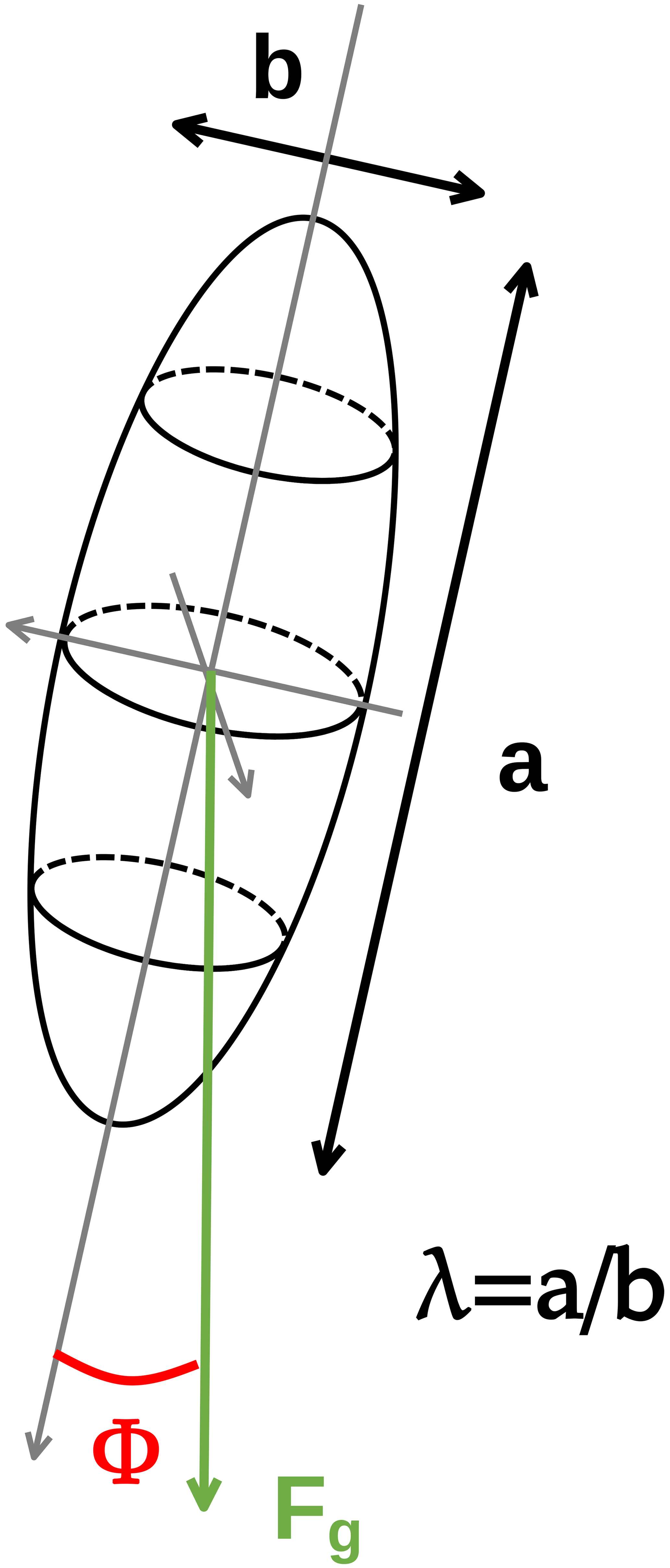
Figure 1 Sketch summarizing the main characteristics of the falling spheroid: polar diameter a, equatorial diameter b, aspect ratio $\mathit{\lambda }=a/b$ and orientation ϕ relative to the gravity force F_g.

Let us now suppose that this spheroid is a material particle with density ρ_p falling under the effect of gravity in a fluid and that this particle is oriented either vertically (ϕ=0) or horizontally ($\mathit{\varphi }=\mathit{\pi }/\mathrm{2}$). In these configurations, no lift force and no torque are exerted by the fluid on the particle, meaning that the particle can fall vertically, with speed u being co-linear to the acceleration of gravity g.

2.2 Method for the calculation of the settling speed in the continuous case

The flow around the settling prolate spheroid (or any object in general) is characterized by the Reynolds number $\mathit{Re}=\frac{\mathit{\rho }UL}{\mathit{\mu }}$, where μ is the dynamic viscosity of the fluid, ρ its mass density, U the speed of the fluid relative to the object and L a characteristic length. The magnitude of the drag force exerted upon the object is typically expressed as $F_{\mathrm{D}}=\frac{\mathrm{1}}{\mathrm{2}}\mathit{\rho }{\mathcal{A}}_{\mathrm{p}}{C}_{\mathrm{D}}\left(\mathit{Re};\mathit{\varphi }\right)U^{\mathrm{2}}$, where 𝒜_p is the cross-flow projected area. This formalism, the most common in aerodynamical studies, is the one used in Mallios et al. (2020), but it has the inconvenience that both the cross-flow projected area 𝒜_p and the drag coefficient C_D depend on the orientation of the object relative to the flow. In Sanjeevi et al. (2022), the Reynolds number Re and the drag coefficient C_D are defined in terms of the volume-equivalent diameter d_eq as follows:

$$\begin{array}{}\text{(5)}& {\displaystyle }\mathit{Re}& {\displaystyle }={\displaystyle \frac{\left|\mathit{u}\right|d_{\mathrm{eq}}\mathit{\rho }}{\mathit{\mu }}}\text{(6)}& {\displaystyle }{F}_{\mathrm{D}}& {\displaystyle }=C_{\mathrm{D}}\left(\mathit{Re},\mathit{\varphi }\right)\times {\displaystyle \frac{\mathrm{1}}{\mathrm{2}}}\mathit{\rho }{\left|\mathit{u}\right|}^{\mathrm{2}}{\displaystyle \frac{\mathit{\pi }}{\mathrm{4}}}{d}_{\mathrm{eq}}^{\mathrm{2}},\end{array}$$

where the drag coefficient C_D(Re,ϕ) depends only on the particle's shape and orientation and on the Reynolds number.

For spheres, Stokes (1851) has proved that for Re≪1 we have $C_{\mathrm{D}}\simeq \frac{\mathrm{24}}{\mathit{Re}}$. This formulation can be extended to prolate spheroids but with a different multiplicative constant:

$$\begin{array}{}\text{(7)}& C_{\mathrm{D}}\simeq {\displaystyle \frac{A^{\mathit{\lambda },\mathit{\varphi }}}{\mathit{Re}}}\mathrm{for}\mathit{Re}\ll \mathrm{1},\end{array}$$

where the expressions for $A^{\mathit{\lambda },\mathit{\varphi }}\left(\mathit{\varphi }\in \left\{\mathrm{0},\frac{\mathit{\pi }}{\mathrm{2}}\right\}\right)$, also known as shape factors, are derived by the exact analytical solution of the Navier–Stokes equation coupled with the continuity equation for the creeping flow of an incompressible viscous fluid past a prolate spheroid (Oberbeck, 1876; Jeffery and Filon, 1922; Chwang and Wu, 1975):

$$\begin{array}{}\text{(8)}& {\displaystyle }{A}^{\mathit{\lambda },\mathit{\varphi }=\mathrm{0}}=\mathrm{64}{\mathit{\lambda }}^{\mathrm{2}/\mathrm{3}}\times e^{\mathrm{3}}{\left[-\mathrm{2}e+\left(\mathrm{1}+e^{\mathrm{2}}\right)\log \left({\displaystyle \frac{\mathrm{1}+e}{\mathrm{1}-e}}\right)\right]}^{-\mathrm{1}},\text{(9)}& {\displaystyle }{A}^{\mathit{\lambda },\mathit{\varphi }=\frac{\mathit{\pi }}{\mathrm{2}}}=\mathrm{64}{\mathit{\lambda }}^{\mathrm{2}/\mathrm{3}}\times \mathrm{2}{e}^{\mathrm{3}}{\left[\mathrm{2}e+\left(\mathrm{3}{e}^{\mathrm{2}}-\mathrm{1}\right)\log \left({\displaystyle \frac{\mathrm{1}+e}{\mathrm{1}-e}}\right)\right]}^{-\mathrm{1}}.\end{array}$$

It is noted that λ→1 and that both $A^{\mathit{\lambda },\mathit{\varphi }=\mathrm{0}}$ and $A^{\mathit{\lambda },\mathit{\varphi }=\frac{\mathit{\pi }}{\mathrm{2}}}$ tend to 24, transforming Eq. (7) to the well-known expression for the drag coefficient of a sphere.

The above drag coefficient expression can be generalized for cases other than creeping flow after multiplication by a correction function 𝒟(Re):

$$\begin{array}{}\text{(10)}& C_{\mathrm{D}}\left(\mathit{Re}\right)={\displaystyle \frac{A^{\mathit{\lambda },\mathit{\varphi }}}{\mathit{Re}}}\mathcal{D}\left(\mathit{Re}\right),\mathrm{with}\underset{\mathit{Re}\to {\mathrm{0}}^{+}}{lim}\mathcal{D}\left(\mathit{Re}\right)=\mathrm{1},\end{array}$$

where function 𝒟 can be named the “drag function”. There is no exact analytical expression of the drag function for the whole range of Reynolds numbers. Mallios et al. (2020) give an expression of this function using theoretical arguments to extend the Clift and Gauvin (1971) empirical formula to prolate spheroids, while Sanjeevi et al. (2022) provides another estimate of 𝒟 based on numerical CFD simulations.

The settling velocity v_∞ can be calculated by the steady-state Newton's law, where the drag force and the buoyancy force counterbalance the gravitational force, leading to a net force equal to zero:

$$\begin{array}{}\text{(11)}& {\displaystyle }{v}_{\mathrm{\infty }}& {\displaystyle }={\displaystyle \frac{\mathrm{4}}{\mathrm{3}}}{\displaystyle \frac{\left({\mathit{\rho }}_{\mathrm{p}}-\mathit{\rho }\right)g{d}_{\mathrm{eq}}^{\mathrm{2}}}{A^{\mathit{\lambda },\mathit{\varphi }}\mathit{\mu }\mathcal{D}\left(\mathit{Re}\right)}},\text{(12)}& {\displaystyle }& {\displaystyle }={\displaystyle \frac{U^{\mathit{\lambda },\mathit{\varphi }}}{\mathcal{D}\left(\mathit{Re}\right)}},\end{array}$$

where $U^{\mathit{\lambda },\mathit{\varphi }}=\frac{\mathrm{4}}{\mathrm{3}}\frac{\left({\mathit{\rho }}_{\mathrm{p}}-\mathit{\rho }\right)g{d}_{\mathrm{eq}}^{\mathrm{2}}}{A^{\mathit{\lambda },\mathit{\varphi }}\mathit{\mu }}$ is the settling velocity of a prolate spheroid with aspect ratio λ and orientation angle ϕ supposing that the Stokes law is verified exactly. On the other hand, v_∞ is the settling speed of the same prolate spheroid taking into account the deviations from the Stokes law, reflected in the 𝒟(Re) drag function. In particular, the Stokes settling speed for the sphere is

$$\begin{array}{}\text{(13)}& U={\displaystyle \frac{\left({\mathit{\rho }}_{\mathrm{p}}-\mathit{\rho }\right)g{d}_{\mathrm{eq}}^{\mathrm{2}}}{\mathrm{18}\mathit{\mu }}}.\end{array}$$

When the particle reaches the terminal settling speed v_∞, we have

$$\begin{array}{}\text{(14)}& \mathit{Re}={\displaystyle \frac{v_{\mathrm{\infty }}{d}_{\mathrm{eq}}\mathit{\rho }}{\mathit{\mu }}}.\end{array}$$

We introduce the Archimedes number Ar (called “virtual Reynolds number” in Mailler et al., 2023c). The Archimedes number is equal to the Reynolds number of a sphere that has the same volume as the prolate spheroid and obeys the Stokes law (Eq. 13):

$$\begin{array}{}\text{(15)}& R={\displaystyle \frac{U{d}_{\mathrm{eq}}\mathit{\rho }}{\mathit{\mu }}}={\displaystyle \frac{\left({\mathit{\rho }}_{\mathrm{p}}-\mathit{\rho }\right)\mathit{\rho }g{d}_{\mathrm{eq}}^{\mathrm{3}}}{\mathrm{18}\mathit{\mu }}}.\end{array}$$

Equation (12) then becomes

$$\begin{array}{}\text{(16)}& {\displaystyle \frac{v_{\mathrm{\infty }}}{U^{\mathit{\lambda },\mathit{\varphi }}}}={\displaystyle }{\left[\mathcal{D}\left(\mathit{Re}\right)\right]}^{-\mathrm{1}}={\left[\mathcal{D}\left({\displaystyle \frac{v_{\mathrm{\infty }}}{U^{\mathit{\lambda },\mathit{\varphi }}}}{\displaystyle \frac{\mathrm{24}}{A^{\mathit{\lambda },\mathit{\varphi }}}}\mathit{Ar}\right)\right]}^{-\mathrm{1}}.\end{array}$$

We now introduce the speed function 𝒮 as

$$\begin{array}{}\text{(17)}& \mathcal{S}={\displaystyle \frac{v_{\mathrm{\infty }}}{U^{\mathit{\lambda },\mathit{\varphi }}}},\end{array}$$

so that 𝒮 is the solution to the fixed-point equation:

$$\begin{array}{}\text{(18)}& {\displaystyle }\mathcal{S}={\left(\mathcal{D}\left({\displaystyle \frac{\mathrm{24}}{A^{\mathit{\lambda },\mathit{\varphi }}}}\mathit{Ar}\cdot \mathcal{S}\right)\right)}^{-\mathrm{1}}.\end{array}$$

As we will see later, solving Eq. (18) permits us to express 𝒮 as a function of the parameters of the problem, in particular of the virtual Reynolds number R. Once this is done, the settling speed can be found as follows:

$$\begin{array}{}\text{(19)}& v_{\mathrm{\infty }}=\mathcal{S}\left(\mathit{Ar}\right)\cdot U^{\mathit{\lambda },\mathit{\varphi }}.\end{array}$$

2.3 Inclusion of the slip-correction factor

For the slip-correction factor, we adopt the formulation of Fan and Ahmadi (2000), based on the adjusted sphere approximation (ASA) introduced by Dahneke (1973). These authors give the following expressions for the slip-correction factors:

$$\begin{array}{}\text{(20)}& \begin{array}{rl}{C}_c^{\mathit{\varphi }}& =\mathrm{1}+{\mathit{Kn}}^{\mathit{\varphi }}\left[\mathrm{1.257}+\mathrm{0.4}\exp \left({\displaystyle \frac{-\mathrm{1.1}}{{\mathit{Kn}}^{\mathit{\varphi }}}}\right)\right],\\ & {\mathit{Kn}}^{\mathit{\varphi }}={\displaystyle \frac{\mathrm{\ell }}{r^{\mathit{\varphi }}}}\left(\mathit{\varphi }\in \left\{\mathrm{0};{\displaystyle \frac{\mathit{\pi }}{\mathrm{2}}}\right\}\right),\end{array}\end{array}$$

where Kn^ϕ is the Knudsen number for orientation ϕ, and $\mathrm{\ell }=\sqrt{\frac{\mathit{\pi }}{\mathrm{8}}}\frac{\mathit{\mu }}{\mathrm{0.4987445}}\frac{\mathrm{1}}{\sqrt{\mathit{\rho }P}}$ is the mean free path of air molecules, with P being the atmospheric pressure (Jennings, 1988).

The radius of the adjusted sphere moving in the polar-axis direction, r^ϕ=0, and that of the adjusted sphere moving in the equatorial direction, $r^{\mathit{\varphi }=\mathit{\pi }/\mathrm{2}}$, are given by

$$\begin{array}{}\text{(21)}& {\displaystyle }\begin{array}{rl}{r}^{\mathit{\varphi }=\mathrm{0}}& ={\displaystyle \frac{\mathrm{1.657}a}{\mathrm{8}\left({\mathit{\lambda }}^{\mathrm{2}}-\mathrm{1}\right)}}\left[{\displaystyle \frac{\mathrm{2}{\mathit{\lambda }}^{\mathrm{2}}-\mathrm{1}}{\sqrt{{\mathit{\lambda }}^{\mathrm{2}}-\mathrm{1}}}}\ln \left(\mathit{\lambda }+\sqrt{{\mathit{\lambda }}^{\mathrm{2}}-\mathrm{1}}\right)+\mathit{\lambda }\right]\\ & \times \left\{\mathrm{2}{E}_{\mathrm{p}}f+{\displaystyle \frac{G_{\mathrm{p}}}{e^{\mathrm{2}}}}\left[e^{\mathrm{2}}\left(\mathrm{4}-\mathrm{2}f\right)-\mathrm{4}+\left(\mathrm{3}-{\displaystyle \frac{\mathit{\pi }}{\mathrm{2}{\mathit{\lambda }}^{\mathrm{2}}}}\right)f\right]\right\},\end{array}\text{(22)}& {\displaystyle }\begin{array}{rl}{r}^{\mathit{\varphi }=\frac{\mathit{\pi }}{\mathrm{2}}}& ={\displaystyle \frac{\mathrm{1.657}a}{\mathrm{16}\left({\mathit{\lambda }}^{\mathrm{2}}-\mathrm{1}\right)}}\left[{\displaystyle \frac{\mathrm{2}{\mathit{\lambda }}^{\mathrm{2}}-\mathrm{3}}{\sqrt{{\mathit{\lambda }}^{\mathrm{2}}-\mathrm{1}}}}\ln \left(\mathit{\lambda }+\sqrt{{\mathit{\lambda }}^{\mathrm{2}}-\mathrm{1}}\right)+\mathit{\lambda }\right]\\ & \times \left\{E_{\mathrm{p}}\left[\mathrm{4}+\left({\displaystyle \frac{\mathit{\pi }}{\mathrm{2}}}-\mathrm{1}\right)f\right]+{\displaystyle \frac{G_{\mathrm{p}}}{e^{\mathrm{2}}}}\left(\mathrm{2}+{\displaystyle \frac{\mathrm{4}{e}^{\mathrm{2}}+\mathit{\pi }-\mathrm{6}}{\mathrm{4}}}f\right)\right\}.\end{array}\end{array}$$

In Eqs. (21)–(22), e is the spheroid's eccentricity as defined in Eq. (2), $E_{\mathrm{p}}=\frac{{\sin }^{-\mathrm{1}}e}{e}$ and $G_{\mathrm{p}}=\frac{\mathrm{1}}{\mathit{\lambda }}-E_{\mathrm{p}}$. Following Mallios et al. (2020), we adopt the value f=0.9113 for the “momentum accommodation coefficient”.

With the inclusion of the slip-correction factor, Eq. (11) is modified as follows:

$$\begin{array}{}\text{(23)}& {\stackrel{\mathrm{̃}}{v}}_{\mathrm{\infty }}={\displaystyle \frac{\mathrm{4}}{\mathrm{3}}}{\displaystyle \frac{C_c^{\mathit{\varphi }}\left({\mathit{\rho }}_{\mathrm{p}}-\mathit{\rho }\right)g{d}_{\mathrm{eq}}^{\mathrm{2}}}{A^{\mathit{\lambda },\mathit{\varphi }}\mathit{\mu }\mathcal{D}\left(\mathit{Re}\right)}}.\end{array}$$

Hereinafter, the variables including the effect of free-slip correction ($C_c^{\mathit{\varphi }}$ in Eq. 23) will be indicated by a tilde ($\stackrel{\mathrm{̃}}{\cdot }$). As such, we introduce the Stokes settling speed including the slip-correction term, ${\stackrel{\mathrm{̃}}{U}}^{\mathit{\varphi }}$, as follows:

$$\begin{array}{}\text{(24)}& {\stackrel{\mathrm{̃}}{U}}^{\mathit{\lambda },\mathit{\varphi }}=C_c^{\mathit{\varphi }}{U}^{\mathit{\lambda },\mathit{\varphi }}.\end{array}$$

With this, in a similar way as in Mailler et al. (2023c), we obtain the following equation:

$$\begin{array}{}\text{(25)}& {\stackrel{\mathrm{̃}}{v}}_{\mathrm{\infty }}=\mathcal{S}\left(\stackrel{\mathrm{̃}}{\mathit{Ar}}\right)\cdot {\stackrel{\mathrm{̃}}{U}}^{\mathit{\lambda },\mathit{\varphi }},\end{array}$$

with

$$\begin{array}{}\text{(26)}& \stackrel{\mathrm{̃}}{\mathit{Ar}}=C_c^{\mathit{\varphi }}{\displaystyle \frac{d_{\mathrm{eq}}^{\mathrm{3}}\mathit{\rho }\left({\mathit{\rho }}_{\mathrm{p}}-\mathit{\rho }\right)g}{\mathrm{18}{\mathit{\mu }}^{\mathrm{2}}}}.\end{array}$$

Function 𝒮 in Eq. (25) is the same as in the case without slip correction defined by Eq. (18).

2.4 Application to the Mallios et al. (2020) drag formulation

At this point, we would like to mention that there are two typos in the equations of Mallios et al. (2020).

1. In the drag coefficient expression for the horizontally oriented particles (their Eqs. 22 and 41), the expressions should be multiplied with the aspect ratio.

2. In the projected area of the horizontally oriented spheroid (their Eq. 45), the expression should be divided by the aspect ratio.

These two modifications cancel each other, since the drag coefficient is multiplied with the projected area for the calculation of the drag force, meaning that the equations governing the settling speed for horizontally oriented spheroids (their Eqs. 50 and 52) are eventually correct. This means that the conclusions of Mallios et al. (2020) are not affected by these typos and that the Corrigendum that was published later by the authors addressing only one of the two typos should not be taken into account since it would lead to erroneous results.

The drag coefficient formulation of Mallios et al. (2020) converted to our notation is

$$\begin{array}{}\text{(27)}& {\displaystyle }{C}_{\mathrm{D},\mathrm{M}\mathrm{20}}^{\mathit{\lambda },\mathit{\varphi }}& {\displaystyle }={\displaystyle \frac{A^{\mathit{\lambda },\mathit{\varphi }}}{\mathit{Re}}}{F}_{\mathrm{cg}}\left({\displaystyle \frac{A^{\mathit{\lambda },\mathit{\varphi }}}{\mathrm{24}}}\mathit{Re}\right),\text{(28)}& {\displaystyle }\mathcal{D}\left(\mathit{Re}\right)& {\displaystyle }=F_{\mathrm{cg}}\left({\displaystyle \frac{A^{\mathit{\lambda },\mathit{\varphi }}}{\mathrm{24}}}\mathit{Re}\right),\end{array}$$

where

$$\begin{array}{}\text{(29)}& F_{\mathrm{cg}}\left(x\right)=\mathrm{1}+\mathrm{0.15}{x}^{\mathrm{0.687}}+{\displaystyle \frac{\mathrm{0.42}x}{\mathrm{24}}}{\left(\mathrm{1}+{\displaystyle \frac{\mathrm{42500}}{x^{\mathrm{1.16}}}}\right)}^{-\mathrm{1}}.\end{array}$$

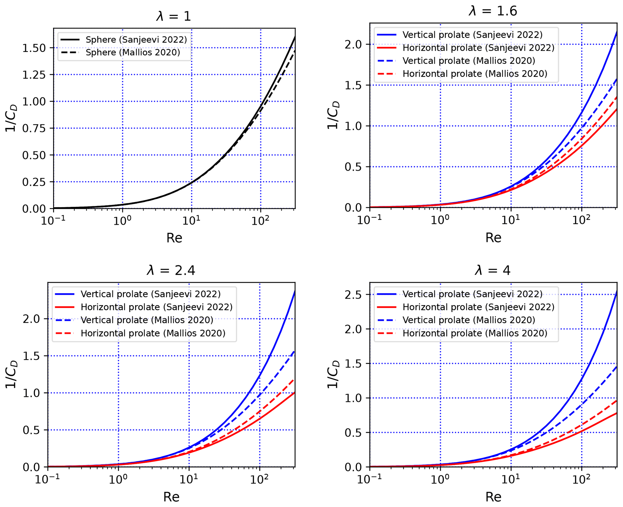
Figure 2 Here we show $\mathrm{1}/C_{\mathrm{D}}$ as a function of Re for (a) λ=1, (b) λ=1.6, (c) λ=2.4 and (d) λ=4. The plots represent $\mathrm{1}/C_{\mathrm{D}}$ rather than C_D to avoid hiding the differences that occur for high Re.

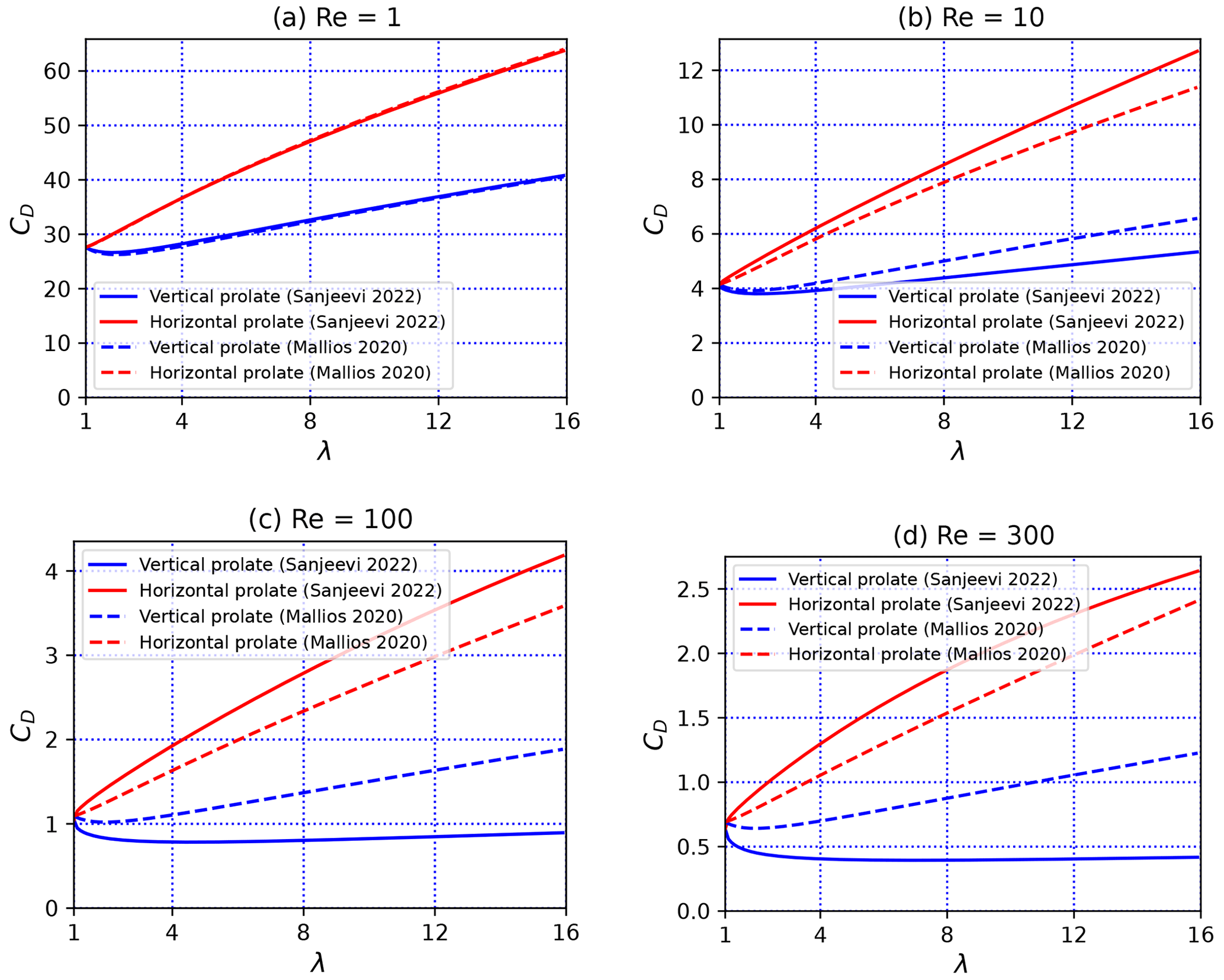
Figure 3 Here we show C_D as a function of λ for (a) Re=1, (b) Re=10, (c) Re=100 and (d) Re=300.

Figures 2 and 3 compare the drag formulation of Mallios et al. (2020) (Eq. 27) to that of Sanjeevi et al. (2022) (see Eq. 35 below). Figure 2a shows that for spherical particles both drag formulations give extremely similar results at least up to Re=300. For prolate spheroidal particles (Fig. 2b, c, d), we observe that the drag formulation of Mallios et al. (2020) is comparable to that of Sanjeevi et al. (2022) for horizontally oriented particles up to Re=300. On the other hand, for vertically oriented particles, we see that substantial differences arise between both formulations, in particular for particles that have a strong aspect ratio. These differences are not problematic for our application because, as we will discuss below, high values of Re are reached only by the coarsest atmospheric particles, and, as shown in, e.g., Mallios et al. (2021), such particles tend to fall with a horizontal orientation. Figure 3 confirms the good agreement between the formulations of Mallios et al. (2020) and Sanjeevi et al. (2022) for both vertical and horizontal orientations at low Reynolds number (Fig. 3a–b). At higher values of Re (Fig. 3c–d), a reasonable degree of agreement persists in the horizontal orientation, but substantial differences arise at high values of Re in the vertical orientation. Generally speaking, for Re≥100, the drag coefficient as calculated from the Mallios et al. (2020) is slightly weaker than the estimate of Sanjeevi et al. (2022) when the particle is oriented horizontally but much stronger than the estimate of Sanjeevi et al. (2022) when the particle is oriented vertically. As we will see below, this will be reflected in stronger discrepancies between both methods for vertically oriented particles than for horizontally oriented particles.

Equation (18) with C_D as expressed in Eq. (27) yields

$$\begin{array}{}\text{(30)}& \mathcal{S}={\left(F_{\mathrm{cg}}\left(\mathit{Ar}\cdot \mathcal{S}\right)\right)}^{-\mathrm{1}}.\end{array}$$

An equivalent fixed-point equation has been solved in Mailler et al. (2023c) (their Eqs. 13 and 16), yielding the following approximated expression for 𝒮(Ar):

$$\begin{array}{}\text{(31)}& \mathcal{S}\left(\mathit{Ar}\right)=\mathrm{1}-{\left[\mathrm{1}+{\left({\displaystyle \frac{\mathit{Ar}}{\mathrm{4.880}}}\right)}^{-\mathrm{0.4335}}\right]}^{-\mathrm{1.905}}.\end{array}$$

As discussed in Mailler et al. (2023c), using this explicit formula instead of numerically resolving Eq. (30) induces a loss of less than 2.5 % in accuracy for Re<1000, which is not critical since the uncertainty in the Clift–Gauvin formula itself (and of other comparable drag-coefficient formulations) is around 7 % when compared to experimental measurements (Goossens, 2019).

This expression of 𝒮 yields the following expression for v_∞ in the absence of slip correction:

$$\begin{array}{}\text{(32)}& \begin{array}{rl}{v}_{\mathrm{\infty }}^{\mathit{\lambda },\mathit{\varphi }}& ={\displaystyle \frac{\mathrm{4}\left({\mathit{\rho }}_{\mathrm{p}}-\mathit{\rho }\right)g{d}_{\mathrm{eq}}^{\mathrm{2}}}{\mathrm{3}\mathit{\mu }{A}^{\mathit{\lambda },\mathit{\varphi }}}}\mathcal{S}\left({\displaystyle \frac{d_{\mathrm{eq}}^{\mathrm{3}}\mathit{\rho }\left({\mathit{\rho }}_{\mathrm{p}}-\mathit{\rho }\right)g}{\mathrm{18}{\mathit{\mu }}^{\mathrm{2}}}}\right),\\ & \mathrm{for}\mathit{\varphi }\in \left\{\mathrm{0};{\displaystyle \frac{\mathit{\pi }}{\mathrm{2}}}\right\},\end{array}\end{array}$$

and in the presence of slip correction:

$$\begin{array}{}\text{(33)}& \begin{array}{rl}{\stackrel{\mathrm{̃}}{v}}_{\mathrm{\infty }}^{\mathit{\lambda },\mathit{\varphi }}& ={\displaystyle \frac{\mathrm{4}{C}_c^{\mathit{\varphi }}\left({\mathit{\rho }}_{\mathrm{p}}-\mathit{\rho }\right)g{d}_{\mathrm{eq}}^{\mathrm{2}}}{\mathrm{3}\mathit{\mu }{A}^{\mathit{\lambda },\mathit{\varphi }}}}\mathcal{S}\left({\displaystyle \frac{C_c^{\mathit{\varphi }}{d}_{\mathrm{eq}}^{\mathrm{3}}\mathit{\rho }\left({\mathit{\rho }}_{\mathrm{p}}-\mathit{\rho }\right)g}{\mathrm{18}{\mathit{\mu }}^{\mathrm{2}}}}\right),\\ & \mathrm{for}\mathit{\varphi }\in \left\{\mathrm{0};{\displaystyle \frac{\mathit{\pi }}{\mathrm{2}}}\right\}.\end{array}\end{array}$$

Figure 4a shows the evaluation of ${\stackrel{\mathrm{̃}}{v}}_{\mathrm{\infty }}^{\mathit{\lambda },\mathit{\varphi }}$ from Eq. (33), and Fig. 4b shows the numerical error due to using Eq. (33) rather than numerically solving the fixed-point Eq.( 30). Both panels of Fig. 4, as well as all the subsequent figures in the study, have been produced using standard atmospheric conditions for air (p=101 325 Pa and T=298.15 K). Dynamic viscosity μ has been calculated following the US Standard Atmosphere (NOAA/NASA/USAF, 1976):

$$\begin{array}{}\text{(34)}& \mathit{\mu }={\displaystyle \frac{\mathit{\beta }{T}^{\frac{\mathrm{3}}{\mathrm{2}}}}{T+S}},\end{array}$$

where $\mathit{\beta }=\mathrm{1.458}\times {\mathrm{10}}^{-\mathrm{6}}$ kg s⁻¹ m⁻¹ K${}^{-\mathrm{1}/\mathrm{2}}$ and S=110.4 K. In these conditions of temperature and pressure and with the molar mass of dry air $M_{\mathrm{a}}=\mathrm{28.9644}\times {\mathrm{10}}^{-\mathrm{3}}$ kg mol⁻¹ (also from the US Standard Atmosphere), the density of air is ρ=1.18 kg m⁻³.

Figure 4a shows that ${\stackrel{\mathrm{̃}}{v}}_{\mathrm{\infty }}^{\mathit{\lambda },\mathit{\varphi }}$ essentially depends on the particle diameter d_eq but also on aspect ratio λ as expected. A closer look at Fig. 4a reveals that, for vertically oriented particles, ${\stackrel{\mathrm{̃}}{v}}_{\mathrm{\infty }}^{\mathit{\lambda },\mathit{\varphi }}$ at first increases with increased aspect ratio, but from λ≃4 this evolution is reversed. Sanjeevi et al. (2022) explain this feature as a tradeoff between the pressure drag and the viscous drag. While the pressure drag continuously decreases with particle elongation (for vertical particles), the viscous drag tends to increase due to the higher surface area of the particle with increasing λ. Figure 4b shows that the error due to using explicit expression (31) induces a difference of less than 2 % for all equivalent diameters up to 10³ µm.

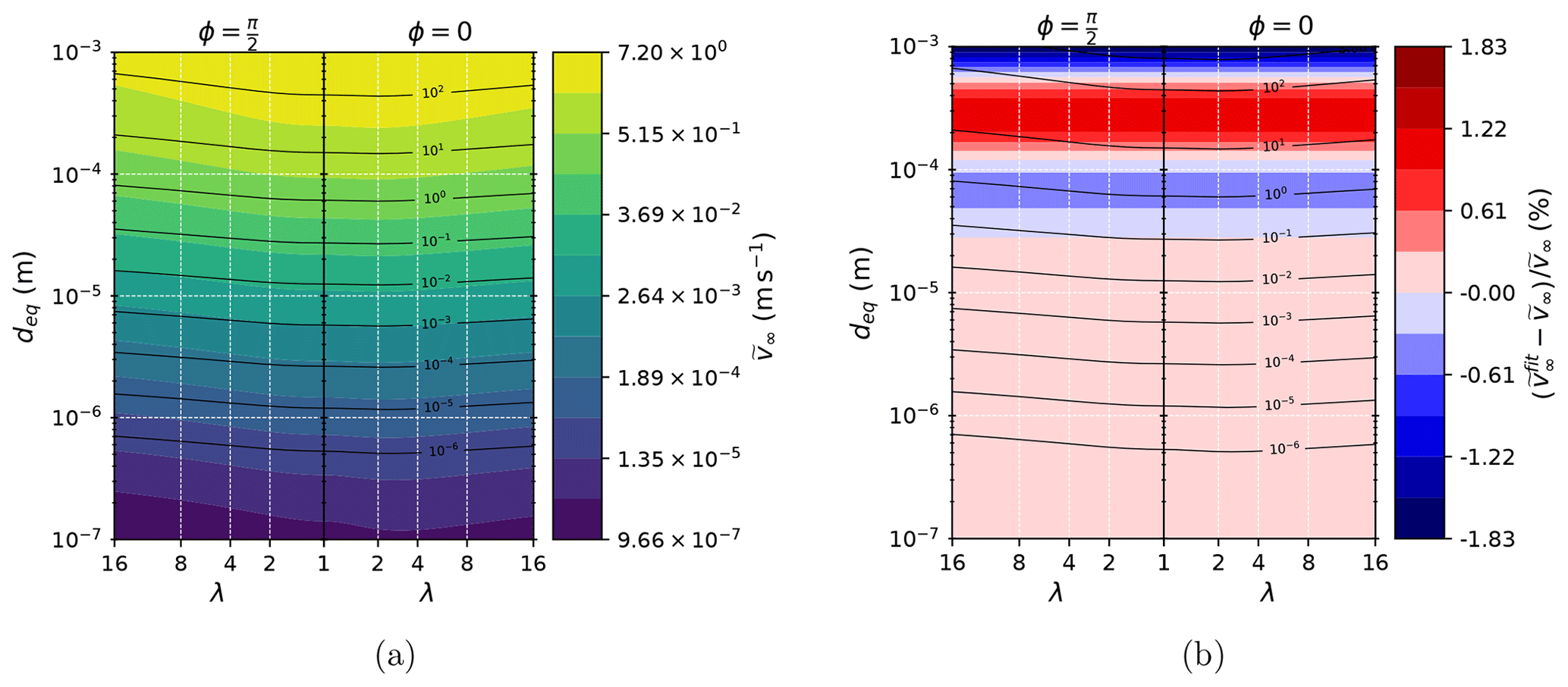
Figure 4 Here we show (a) ${\stackrel{\mathrm{̃}}{v}}_{\mathrm{\infty }}^{\mathit{\lambda },\mathit{\varphi }}$ as a function of d_eq and λ for $\mathit{\varphi }=\frac{\mathit{\pi }}{\mathrm{2}}$ (a) and ϕ=0 (b), using Eq. (31) to estimate 𝒮 and (b) error (in %) committed using the explicit expression Eq. (31) instead of numerically solving Eq. (30). Contours in (a) and (b) represent the Reynolds number. This figure has been produced using standard atmospheric conditions (p=101 325 Pa, T=298.15 K).

2.5 Sensitivity of the settling speed to large-particle correction, eccentricity correction and slip correction

Figure 5 shows the effects of large-particle correction (Fig. 5a), eccentricity correction (Fig. 5b) and slip correction (Fig. 5c) on the settling speed, showing that large-particle correction begins to be significant ($<-\mathrm{5}$ %) for particles with d_eq>30 µm. On the contrary, slip correction is significant (>5 %) only for particles with d_eq<3–5 µm (depending on particle eccentricity). For lower pressure values (p≃200 hPa) representative of the higher troposphere or lower stratosphere, slip correction increases due to the longer mean free path for air particles in thinner air. At these altitudes, slip correction reaches 5 % for particles with d_eq<8–15 µm (not shown), while large-particle corrections also reach −5 % for particles with d_eq>30 µm (not shown). Total correction to the Stokes velocity of the volume-equivalent sphere (including the effect of eccentricity, slip correction, and large-particle correction) is shown in Fig. 6, revealing that the magnitude of the effect behaves differently for horizontal and vertical particles. Horizontal particles always fall more slowly than their volume-equivalent sphere. For aspect ratio λ>2, the difference is around 10 %, showing a possible interest of this difference from a modeling point of view. For vertically oriented particles, except for the smaller ones (influenced by slip-correction factors), the difference in ${\stackrel{\mathrm{̃}}{v}}_{\mathrm{\infty }}$ due to particle eccentricity does not exceed ±10 % until λ≃7. Figure 6, including both eccentricity and large-particle effects, shows the difference between the model we propose here (Eq. 33) and the expression typically used in chemistry transport models, assuming particles to be spherical and not taking into account large-particle correction. Consistently with Fig. 5a–b, it shows that these effects need to be into account when λ>2 and/or d_eq>50 µm and that the eccentricity effect is much stronger for horizontally oriented particles than for vertically oriented particles.

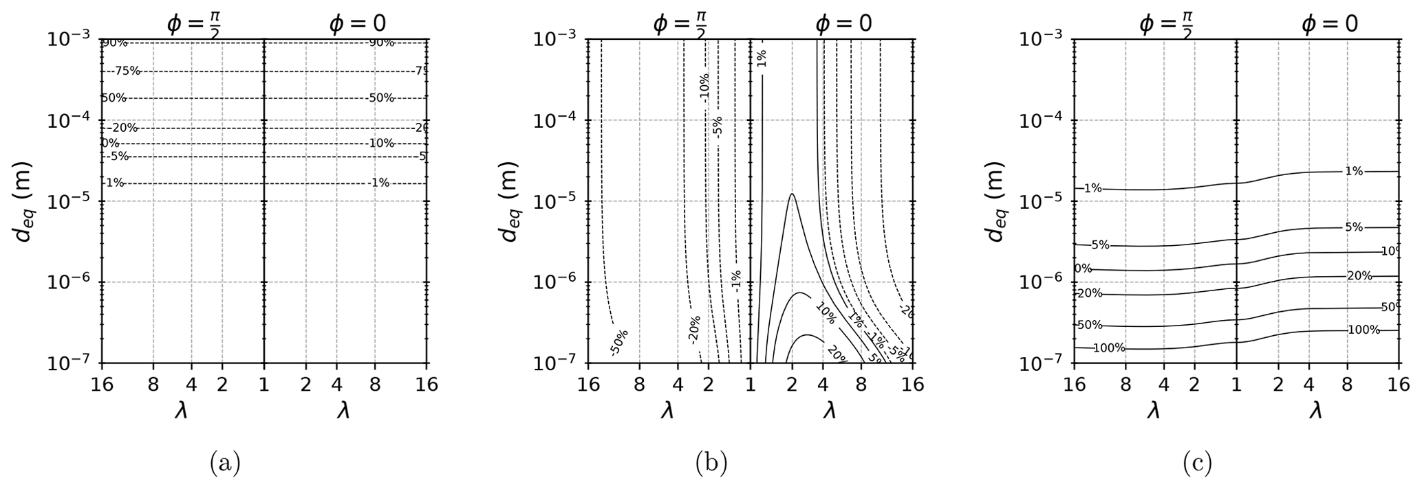
Figure 5 (a) Large-particle correction $\frac{{\stackrel{\mathrm{̃}}{v}}_{\mathrm{\infty }}-{\stackrel{\mathrm{̃}}{U}}^{\mathit{\lambda },\mathit{\varphi }}}{{\stackrel{\mathrm{̃}}{U}}^{\mathit{\lambda },\mathit{\varphi }}}$, (b) eccentricity correction $\frac{{\stackrel{\mathrm{̃}}{v}}_{\mathrm{\infty }}\left(\mathit{\lambda };d_{\mathrm{eq}}\right)-{\stackrel{\mathrm{̃}}{v}}_{\mathrm{\infty }}\left(\mathit{\lambda }=\mathrm{0};d_{\mathrm{eq}}\right)}{{\stackrel{\mathrm{̃}}{v}}_{\mathrm{\infty }}\left(\mathit{\lambda }=\mathrm{0};d_{\mathrm{eq}}\right)}$ and (c) slip-correction $\frac{{\stackrel{\mathrm{̃}}{v}}_{\mathrm{\infty }}\left(\mathit{\lambda };d_{\mathrm{eq}}\right)-v_{\mathrm{\infty }}\left(\mathit{\lambda };d_{\mathrm{eq}}\right)}{v_{\mathrm{\infty }}\left(\mathit{\lambda };d_{\mathrm{eq}}\right)}$. The values in all three panels are given in percentages (contours). The figure has been produced using standard atmospheric conditions (p=101 325 hPa, T=298.15 K).

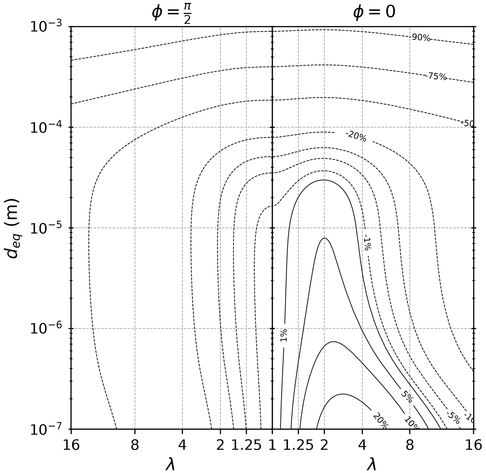
Figure 6 Total correction to the slip-corrected Stokes speed for a volume-equivalent sphere, $\frac{{\stackrel{\mathrm{̃}}{v}}_{\mathrm{\infty }}-{\stackrel{\mathrm{̃}}{U}}^{\mathit{\lambda },\mathit{\varphi }}}{{\stackrel{\mathrm{̃}}{U}}^{\mathit{\lambda },\mathit{\varphi }}}$. This figure has been produced using standard atmospheric conditions (p=101 325 Pa, T=298.15 K).

3 Comparison with the Sanjeevi et al. (2022) drag formulation

3.1 Expression of the settling speed from the Sanjeevi et al. (2022) drag formulation

Sanjeevi et al. (2022) authors suggest the following form:

$$\begin{array}{}\text{(35)}& \begin{array}{rl}{C}_{\mathrm{D},\mathrm{S}\mathrm{22}}^{\mathit{\lambda },\mathit{\varphi }}& =\left({\displaystyle \frac{A^{\mathit{\lambda },\mathit{\varphi }}}{\mathit{Re}}}+{\displaystyle \frac{a_{\mathrm{2}}^{\mathit{\lambda },\mathit{\varphi }}}{{\mathit{Re}}^{a_{\mathrm{3}}^{\mathit{\lambda },\mathit{\varphi }}}}}\right)e^{-a_{\mathrm{4}}^{\mathit{\lambda },\mathit{\varphi }}\mathit{Re}}\\ & +a_{\mathrm{5}}^{\mathit{\lambda },\mathit{\varphi }}\left(\mathrm{1}-e^{-a_{\mathrm{4}}^{\mathit{\lambda },\mathit{\varphi }}\mathit{Re}}\right),\mathrm{for}\mathit{\varphi }\in \left\{\mathrm{0};{\displaystyle \frac{\mathit{\pi }}{\mathrm{2}}}\right\}.\end{array}\end{array}$$

While $a_{\mathrm{3}}^{\mathit{\lambda },\mathit{\varphi }}<\mathrm{1}$, these equations guarantee that $C_{\mathrm{D}}^{\mathit{\lambda },\mathit{\varphi }}=\frac{A^{\mathit{\lambda },\mathrm{\Phi }}}{\mathit{Re}}$ is the dominant term for Re≪1. Coefficients $a_{\mathrm{2}}^{\mathit{\lambda },\mathit{\varphi }}$ to $a_{\mathrm{5}}^{\mathit{\lambda },\mathit{\varphi }}$ have been determined empirically by Sanjeevi et al. (2022), and these authors give the necessary expressions, dependent on λ, in their Eqs. (11)–(12) and Table 2. Therefore, combining Eq. (35) with the expressions of the a_i coefficients, the above elements permit us to completely express the drag coefficient C_D as a function of Re, the aspect ratio λ and the attack angle ϕ for all the falling spheroids.

The expression of 𝒟 (Eq. 10) from the expressions of Sanjeevi et al. (2022) (Eq. 35) is as follows, with either ϕ=0 or $\mathit{\varphi }=\frac{\mathit{\pi }}{\mathrm{2}}$:

$$\begin{array}{}\text{(36)}& \begin{array}{rl}\mathcal{D}& =\left(\mathrm{1}+{\displaystyle \frac{a_{\mathrm{2}}^{\mathit{\lambda },\mathit{\varphi }}}{A^{\mathit{\lambda },\mathit{\varphi }}}}{\left(\mathit{Re}\right)}^{\mathrm{1}-a_{\mathrm{3}}^{\mathit{\lambda },\mathit{\varphi }}}\right)e^{-a_{\mathrm{4}}^{\mathit{\lambda },\mathit{\varphi }}\mathit{Re}}\\ & +{\displaystyle \frac{a_{\mathrm{5}}^{\mathit{\lambda },\mathit{\varphi }}}{A^{\mathit{\lambda },\mathit{\varphi }}}}\mathit{Re}\left(\mathrm{1}-e^{-a_{\mathrm{4}}^{\mathit{\lambda },\mathit{\varphi }}\mathit{Re}}\right).\end{array}\end{array}$$

With this expression of 𝒟, it is possible to numerically solve Eq. (18) to obtain the values of 𝒮 as a function of λ, $\mathit{\varphi }\in \left\{\mathrm{0};\mathit{\pi }/\mathrm{2}\right\}$ and R. In Mailler et al. (2023c), we see that for spherical particles it is possible to express 𝒮 as a function of R with a high degree of accuracy as follows:

$$\begin{array}{}\text{(37)}& \mathcal{S}\left(\mathit{Ar}\right)\simeq -{\left(\mathrm{1}+e^{-c_{\mathrm{1}}^{\mathit{\varphi }}\left(\mathit{\lambda }\right)\left(\ln \mathit{Ar}-c_{\mathrm{2}}^{\mathit{\varphi }}\left(\mathit{\lambda }\right)\right)}\right)}^{c_{\mathrm{3}}^{\mathit{\varphi }}\left(\mathit{\lambda }\right)},\end{array}$$

We have found that approximated expressions of the following form hold for the $c_i^{\mathit{\varphi }}$ coefficients:

$$\begin{array}{}\text{(38)}& {\displaystyle }\begin{array}{rl}{c}_i^{\mathit{\varphi }}& =A_i+B_i^{\mathit{\varphi }}e\mathit{\lambda }+C_i^{\mathit{\varphi }}\left(\mathit{\lambda }-\mathrm{1}\right)+D_i^{\mathit{\varphi }}e+E_i^{\mathit{\varphi }}{\displaystyle \frac{e}{\mathit{\lambda }}}\\ & +F_i^{\mathit{\varphi }}{\left(e\mathit{\lambda }\right)}^{\mathrm{2}}\mathrm{for}{c}_{\mathrm{1},\mathrm{2},\mathrm{3}}^{\mathrm{0}}\text{and for}{c}_{\mathrm{1},\mathrm{2}}^{\mathit{\pi }/\mathrm{2}},\end{array}\text{(39)}& {\displaystyle }\begin{array}{rl}{c}_{\mathrm{3}}^{\mathit{\pi }/\mathrm{2}}& =A_{\mathrm{3}}+B_{\mathrm{3}}^{\mathit{\pi }/\mathrm{2}}e\mathit{\lambda }+C_{\mathrm{3}}^{\mathit{\pi }/\mathrm{2}}\left(\mathit{\lambda }-\mathrm{1}\right)+D_{\mathrm{3}}^{\mathit{\pi }/\mathrm{2}}e\\ & +E_{\mathrm{3}}^{\mathit{\pi }/\mathrm{2}}{\displaystyle \frac{e}{\mathit{\lambda }}}+F_{\mathrm{3}}^{\mathit{\pi }/\mathrm{2}}{\left(e\mathit{\lambda }\right)}^{\mathrm{4}}.\end{array}\end{array}$$

The values of A_i, $B_i^{\mathit{\varphi }}$, $C_i^{\mathit{\varphi }}$, $D_i^{\mathit{\varphi }}$, $E_i^{\mathit{\varphi }}$ and $C_i^{\mathit{\varphi }}$ for $i\in \left\{\mathrm{1};\mathrm{2};\mathrm{3}\right\}$ and $\mathit{\varphi }\in \left\{\mathrm{0};\mathit{\pi }/\mathrm{2}\right\}$ are given in Table 1.

Table 1 Values of the coefficients in Eqs. (38)–(39).

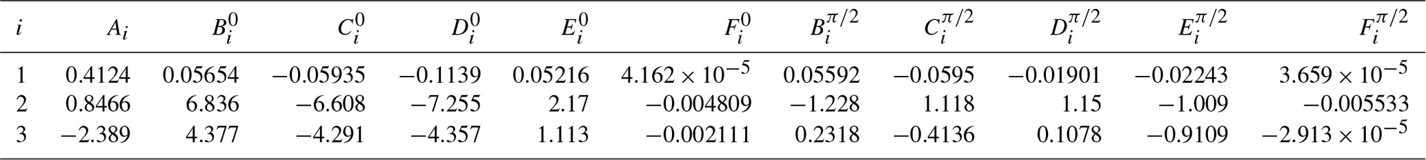
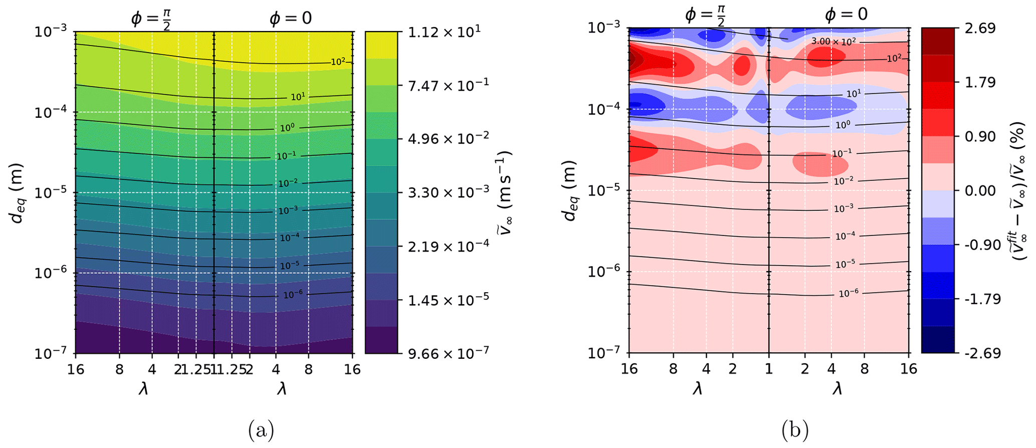
Figure 7 Here we show (a) ${\stackrel{\mathrm{̃}}{v}}_{\mathrm{\infty }}^{\mathit{\lambda },\mathit{\varphi }}$ as a function of d_eq and λ for $\mathit{\varphi }=\frac{\mathit{\pi }}{\mathrm{2}}$ (a) and ϕ=0 (b) using Eq. (37) and (b) error (in %) committed using the explicit expression Eq. (37) instead of numerically solving Eq. (18). Contours in (a) and (b) represent the Reynolds number. This figure has been produced using standard atmospheric conditions (p=101 325 Pa, T=298.15 K).

Figure 7a shows the evaluation of ${\stackrel{\mathrm{̃}}{v}}_{\mathrm{\infty }}^{\mathit{\lambda },\mathit{\varphi }}$ using 𝒮 from Eq. (37), and Fig. 7b shows the numerical error due to using Eq. (37) rather than numerically solving Eq. (18). Figure 7a shows a behavior very similar to the Mallios et al. (2020) formulation (a more detailed comparison of the results will be provided below). Figure 7b shows that the error attributable to the numerical fit of 𝒮 by Eq. (37) is very small, i.e., less than 2.6 % in all the represented domain. Therefore, there is no inconvenience in using this approximated expression for 𝒮.

3.2 Comparison of the speed expressions from Mallios et al. (2020) and Sanjeevi et al. (2022)

Figure 8 shows the relative difference between the estimation of ${\stackrel{\mathrm{̃}}{v}}_{\mathrm{\infty }}$ from the Sanjeevi et al. (2022) drag formulation and from the Mallios et al. (2020) drag formulation. Up to $d_{\mathrm{eq}}\simeq {\mathrm{10}}^{-\mathrm{4}}$ m, the difference between both formulations is below or around 2 %. Differences are more substantial for $d_{\mathrm{eq}}>{\mathrm{10}}^{-\mathrm{4}}$ m and for the vertically oriented particles. For horizontally oriented particles, differences stay below or around 10 % up to $d_{\mathrm{eq}}={\mathrm{10}}^{-\mathrm{3}}$ m, which is close to the uncertainty range of both the Clift and Gauvin (1971) drag formulation (see Goossens, 2019) and the Sanjeevi et al. (2022) formulation. This is particularly interesting since, as shown by Mallios et al. (2021), for reasons of stability, the large and elongated particles with diameter $>{\mathrm{10}}^{-\mathrm{4}}$ m tend to be aligned horizontally. In contrast, for vertically falling particles, error builds up rapidly and is in excess of 50 % for the biggest and most elongated particles. This tends to show that the accuracy of the Mallios et al. (2020) model is excellent (close to 2 %) for all particle diameters with $d_{\mathrm{eq}}<{\mathrm{10}}^{-\mathrm{4}}$ m and good (close to 10 %) for all the horizontally oriented particles with $d_{\mathrm{eq}}<{\mathrm{10}}^{-\mathrm{3}}$ m. All in all, if we suppose that the Sanjeevi et al. (2022) is valid in the range claimed by these authors (λ<16 and Re<2000), our results show that the accuracy of the theoretical formulation of Mallios et al. (2020) and its application to an explicit expression of ${\stackrel{\mathrm{̃}}{v}}_{\mathrm{\infty }}$ (Eq. 33) is suitable for the use in atmospheric sciences for all the atmospheric aerosol that can be reasonably assumed to have a spherical or prolate spheroidal shape.

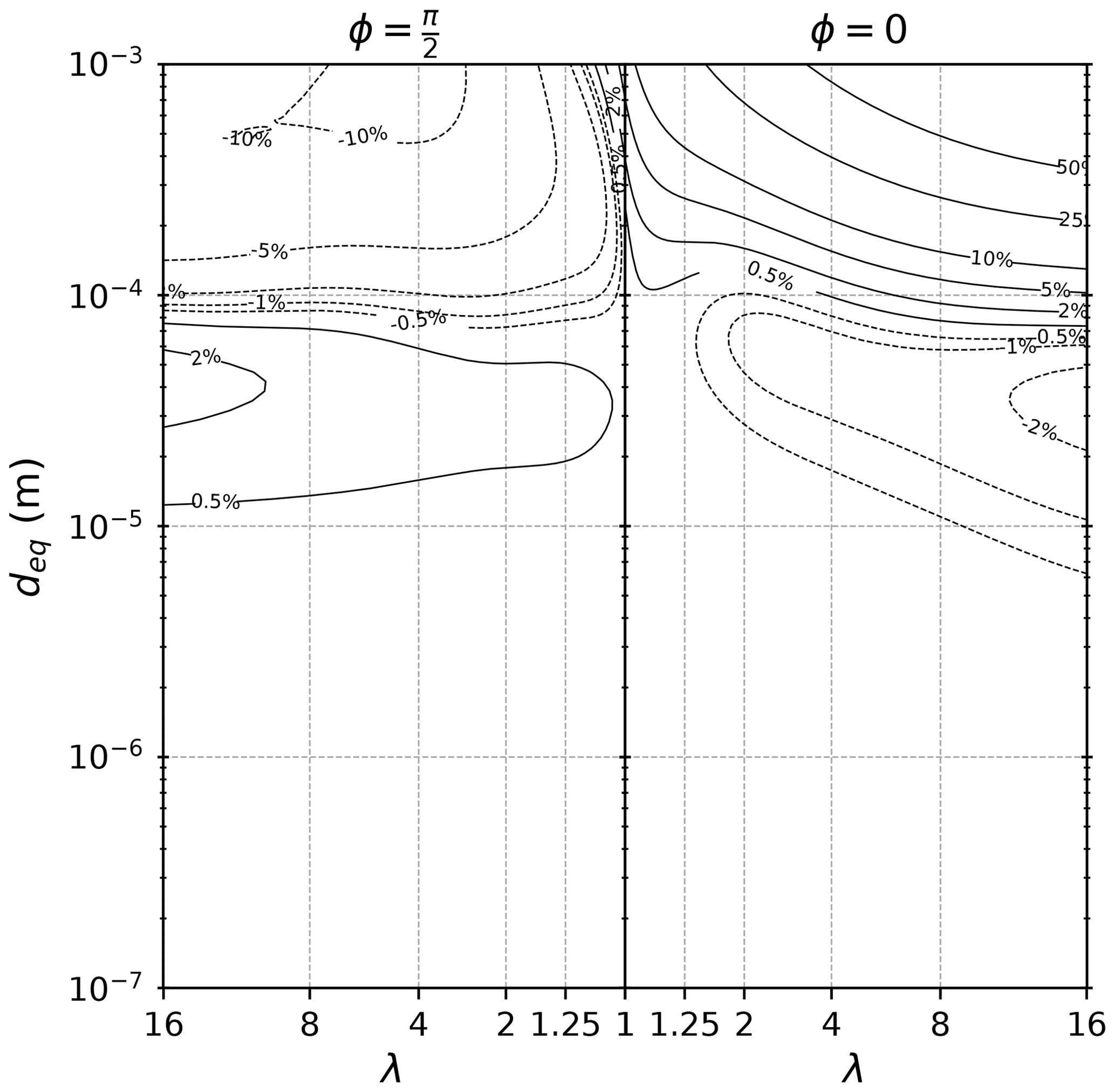
Figure 8 Relative difference $\left(\frac{{\stackrel{\mathrm{̃}}{v}}_{\mathrm{\infty }}^{Sj\mathrm{22}}-{\stackrel{\mathrm{̃}}{v}}_{\mathrm{\infty }}^{\mathrm{M}\mathrm{20}}}{{\stackrel{\mathrm{̃}}{v}}_{\mathrm{\infty }}^{\mathrm{M}\mathrm{20}}}\right)$ (in %) between the settling speed estimated from the Sanjeevi et al. (2022) formulation (Eq. 37) and from the Mallios et al. (2020) formulation (Eq. 31). This figure has been produced using standard atmospheric conditions (p=101 325 Pa, T=298.15 K).

4 Implementation in AerSett v2.0.2

Equation (33), along with Eqs. (8)–(9) to express A^λ,ϕ, Eqs. (20)–(22) to express $C_c^{\mathit{\varphi }}$ and Eq. (31) giving the expression of function 𝒮, gives the expression of the settling speed of a falling particle as a function of the following variables:

• d_eq, the mass-equivalent diameter of the particle;

• ρ_p, the density of the particle;

• ρ_a, the density of air;

• μ, the dynamic viscosity of air;

• ℓ, the mean free path of air molecules;

• λ, the aspect ratio of the particle;

• $\mathit{\varphi }\in \left\{\mathrm{0}\mathit{°};\mathrm{90}\mathit{°}\right\}$, the attack angle of the particle.

Equation (33) extends the method exposed for spherical particles in Mailler et al. (2023c) to the calculation of the settling speed of prolate spheroidal aerosols. This permits us to generalize the AerSett module to the calculation of the settling speed of prolate spheroidal aerosol. Here we present this implementation and qualify the results of AerSett 2.0.2 in terms of accuracy and numerical efficiency (Table 2).

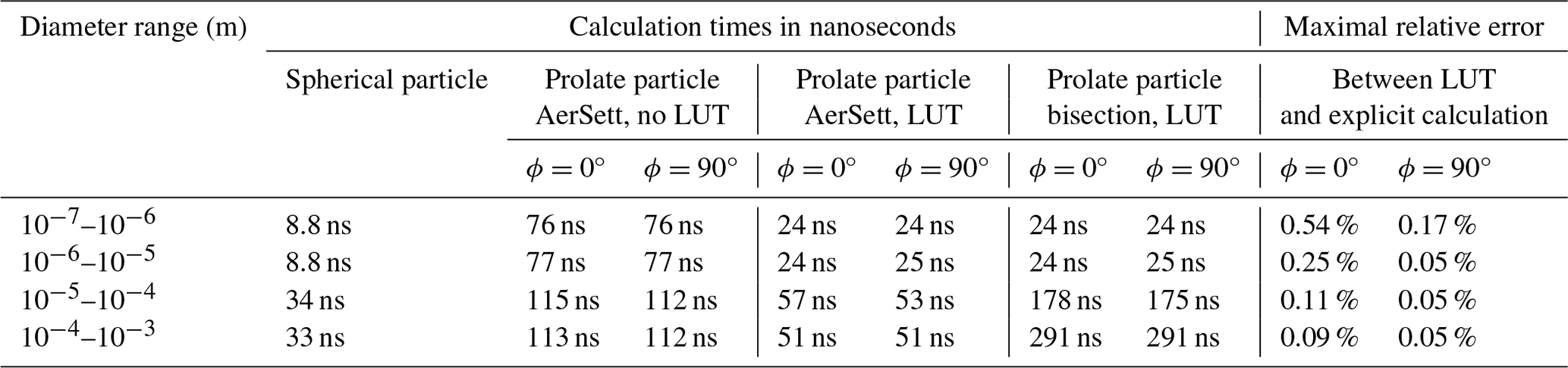
The US Standard Atmosphere (NOAA/NASA/USAF, 1976) has been used as a typical profile for pressure and density. The mass-equivalent diameters of the particles span the range from 10⁻⁷ to 10⁻³ m, which has been divided into four intervals (column 1 of Table 2). The mean calculation times for each diameter range are evaluated by calling the calculation routine 10⁷ times on a random sample of 10⁷ triplets of diameter, aspect ratio (between 1 and 16) and altitude (between 1 and 12 000 m a.s.l.) in the case of spheres and prolate spheroids (columns 2–4 of Table 2).

To speed up the calculations, the values of $\frac{r^{\mathit{\varphi }}}{a}$ (Eqs. 21–22) and A^λ,ϕ (Eqs. 8–9) for $\mathit{\varphi }\in \left\{\mathrm{0}\mathit{°};\mathrm{90}\mathit{°}\right\}$ and for $\mathrm{1}<\mathit{\lambda }<\mathrm{16}$ with a step of 0.01 on λ are calculated once and for all in the initialization phase and stored in arrays to be used at each call of the calculation routine. This initialization phase takes less than 1 ms on a laptop and needs to be performed only once. The change in performance due to this precalculation of some parameters can be seen in columns 5–6 of Table 2. Finally, columns 9–10 indicate the percentage error due to the use of lookup tables for Eqs. (8)–(9) and (21)–(22) instead of the formal calculations.

Table 2 shows that the computation time for the settling speed of a prolate particle with AerSett is longer than for a spherical particle, even when a lookup table is used instead of Eqs. (8)–(9) and (21)–(22). However, the use of the lookup table strongly reduces this additional cost. Once the lookup table is used, the residual extra cost of the spheroidal calculation (columns 5–6) compared to the spherical calculation (column 2) is around 15 ns for the small particles and around 20 ns for the largest ones. The effect of the lookup table on the accuracy of the calculation (columns 9–10) is below 1 %, which is negligible in comparison to the physical uncertainties in the problem.

To compare the efficiency of the method we present here, columns 7–8 give the calculation time to obtain the same result (within an accuracy ±2 %) with the previously available method (bisection method applied to Eqs. (51)–(52) of Mallios et al., 2020). As in Mailler et al. (2023c), large-particle correction is applied only when $\stackrel{\mathrm{̃}}{R}>\mathrm{0.0232}$ because for smaller $\stackrel{\mathrm{̃}}{R}$ it changes the value of the settling speed by less than 1 %. For particles with d_eq>10  µm, large-particle correction is applied, and in this case the calculation time using the explicit expression of 𝒮 (Eq. 31) is 3 to 6 times shorter than the explicit resolution of the fixed-point equation. As expected from the results of Mailler et al. (2023c), the difference between the result from the application of Eq. (31) and the explicit resolution of the fixed-point equation by bisection is less than 2 % throughout the entire range ($d_{\mathrm{eq}}<{\mathrm{10}}^{-\mathrm{3}}$ m and $\mathrm{1}<\mathit{\lambda }<\mathrm{16}$).

Table 2 Average calculation times to obtain the settling speed of spherical and prolate particles using AerSett (columns 2–6) and using a bisection method (columns 7–8) as a function of the range of mass-equivalent diameter (column 1). Columns 9–10 give the percentage error due to the use of lookup tables (LUTs) for Eqs. (21)–(22) and (8)–(9) instead of the formal calculations.
The tests were performed on a laptop with an Intel Core i7-1165G7 CPU.

5 Conclusions

We found that Eq. (25) is valid to express the settling speed of solid aerosol particles in the atmosphere, where the function 𝒮 depends only on the shape and orientation of the particle. The precise expression of 𝒮 is related to the C_D=f(Re) relationship through Eq. (18).

We provide two expressions of 𝒮 for prolate spheroids. The first one (Eq. 31) is derived from the theoretical drag formulation of Mallios et al. (2020) and a natural extension of the similar function for spheres (Mailler et al., 2023c). The second one, Eq. (37), with coefficients as expressed in Table 1, is based on the CFD results of Sanjeevi et al. (2022). Agreement between these two expressions (Fig. 7) is excellent for all prolate spheroids in the atmosphere with $d_{\mathrm{eq}}<{\mathrm{10}}^{-\mathrm{4}}$ m, with differences below or around 2 %. Since the approaches of Mallios et al. (2020) and Sanjeevi et al. (2022) are completely different and independent, these results provide a robust validation of both drag formulations in the Stokes and transition regimes.

For higher diameters, differences are still moderate for the horizontally oriented particles (below or around 10 %) but much stronger for vertically oriented particles (up and beyond 50 %). However, this is not relevant for atmospheric modeling since it has been shown by Mallios et al. (2021) that large atmospheric particles fall in horizontal orientation under the action of the aerodynamic torque. Therefore, the drag formulation based on the results of Mallios et al. (2020), more simple than that of Sanjeevi et al. (2022), applies to all the relevant range for atmospheric particles, meaning that we propose the following method to estimate the settling speed of prolate aerosols:

1. calculate r^ϕ from Eqs. (21)–(22);

2. calculate $C_c^{\mathit{\varphi }}$ from Eq. (20);

3. calculate ${\stackrel{\mathrm{̃}}{U}}^{\mathit{\lambda },\mathit{\varphi }}$ from Eq. (24) and Eqs. (8)–(9);

4. calculate $\stackrel{\mathrm{̃}}{\mathit{Ar}}$ from Eq. (26);

5. finally, calculate ${\stackrel{\mathrm{̃}}{v}}_{\mathrm{\infty }}$ from Eq. (25).

AerSett v2.0.2 (Mailler et al., 2023a) provides a Fortran implementation of these equations that is ready to use for atmospheric modelers. When large-particle correction is requested, the calculation times obtained with this formulation are 3 to 6 times shorter than previously available methods such as bisection used in Mallios et al. (2020). We found that storing the output of Eqs. (8)–(9) and (21)–(22) in a precalculated lookup table permits us to reduce the computational time by more than half while changing the numerical results by less than 1 %. The present method could be easily extended to particles made of porous materials by considering that a particle made of a material of density ρ_m having porosity ϕ can be treated as a dense material with effective density ${\mathit{\rho }}_{\mathrm{p}}={\mathit{\rho }}_{\mathrm{m}}\left(\mathrm{1}-\mathit{\varphi }\right)$.

From a geophysical point of view and regarding the issue of giant dust, as discussed in Mallios et al. (2021), when the electric field is small or non-existent such large particles tend to fall with a horizontal orientation ($\mathit{\varphi }=\mathit{\pi }/\mathrm{2}$) under the effect of the aerodynamic torque, in which case our results indicate that their settling speed would be reduced by about 10 % for an aspect ratio λ=2 and by about 20 % for λ=4. This effect may be significant, but it is not strong enough to explain the long atmospheric lifetime of giant dust. However, as shown by Yang et al. (2013), there is observational evidence of shape-induced gravitational sorting during the voyage of dust particles over the Atlantic. Our results give a way to calculate efficiently the shape-induced differences in the settling speed of aerosols, and thereby represent a step towards reproducing such effects of shape-induced gravitational sorting in general circulation models or in chemistry transport models.

From methods based on mechanics and statistical physics, Mallios et al. (2021) have determined the probability density functions (PDFs) for particle attack angles as a function of their aspect ratio, the other characteristics of the particle and the fluid (assuming particles shaped as prolate spheroids). Based on these PDFs the authors have calculated the average attack angle of particles with different sizes. They showed that particles with sizes less than ≃2 µm are in principle randomly oriented, while particles with sizes larger than ≃20 µm tend to fall with an essentially horizontal orientation. Therefore, in their present formulation, our results only permit the explicit calculation of the settling speed of giant dust particles with d_eq>20 µm, assuming that their orientation is essentially horizontal. In principle, the results presented here are based on non-dimensional relationships and should also be valid for rigid prolate bodies settling in liquids in the same ranges of Reynolds tested here (from Re≪1 to Re≃300). In geosciences, this could be of interest for the settling of sediments in lakes or oceans, for example.

A future line of work is to find theoretical and/or heuristic ways to extend our findings to the intermediate orientations and to obtain an expression of the instant settling speed for each possible attack angle. Following this, this expression could be integrated at all attack angles (weighted by the PDF of the attack angle) to obtain the resulting average settling speed for a given particle depending on particle shape and fluid characteristics and for all possible sizes of atmospheric aerosols. This will be the main topic of future work that is currently underway.

Other limitations of the present work include the assumption of prolate spheroidal shape for the dust particles. Taking into account the fact that expressions comparable to Eqs. (8)–(9) exist for the case of oblate spheroids, we see no particular obstacles in generalizing the approach developed in Mallios et al. (2020) and in the present article to the case of oblate spheroids. The case of triaxial spheroids or of other more irregular shapes is still out of reach with the methods developed here.