the Creative Commons Attribution 4.0 License.
the Creative Commons Attribution 4.0 License.
 | 17 Jul 2024
The CHIMERE chemistry-transport model v2023r1
Laurent Menut
Arineh Cholakian
Romain Pennel
Guillaume Siour
Sylvain Mailler
Myrto Valari
Lya Lugon
Yann Meurdesoif
A new version of the CHIMERE model is presented. This version contains both computational and physico-chemical changes. The computational changes make it easy to choose the variables to be extracted as a result, including values of maximum sub-hourly concentrations. Performance tests show that the model is 1.5 to 2 times faster than the previous version for the same setup. Processes such as turbulence, transport schemes and dry deposition have been modified and updated. Optimization was also performed for the management of emissions such as anthropogenic and mineral dust. The impact of fires on wind speed, soil properties and leaf area index (LAI) was added. Pollen emissions, transport and deposition were added for birch, ragweed, olive and grass. The model is validated with a simulation covering Europe with a 60 km × 60 km resolution and the entire year of 2019. Results are compared to various measurements, and statistical scores show that the model provides better results than the previous versions.
- Article
(1426 KB) - Full-text XML
- BibTeX
- EndNote


Chemistry-transport modelling is useful for the analysis and forecast of atmospheric pollution events. Regional deterministic models have proven their value for studies about climate change, emissions regulations, day-to-day pollution evolution and health effects, among many other topics. These models have to both be accurate and have a low computational time.
The CHIMERE chemistry-transport model has been under continuous development since 1999. Several versions have been released as open-source software since the first one. The model is now used for analysis and forecast in many institutes, research laboratories and private companies. For the last 10 years, releases were distributed at a frequency of a new major one every 3 years. Each version of the model is distributed with other ancillary codes. These ancillary codes are developed by the same team and are intended to help users prepare the input data required for a simulation. These codes are detailed in the documentation. The model is distributed with other codes dedicated to helping users prepare for forcings such as weather and broadcasts. The model is also distributed with a test case to show the user the necessary input data and what the model's output looks like.
The first version with full documentation of all the processes taken into account in the model was version 2014. It included the possibility of reading emission fluxes from fires, calculated using a specific model in pre-processing; reading daily satellite data of fire radiative power and burnt areas; and converting this information into chemical species hourly fluxes using additional information, such as vegetation type and related fuel load for each. It also includes the Statewide Air Pollution Research Center (SAPRC) chemical mechanism (Carter, 2010), an adaptive time step and the new datasets for the chemical boundary conditions (Menut et al., 2013). Version 2017 (Mailler et al., 2017) added the possibility of using a hemispheric domain (and the way to manage the grid and the transports schemes), the new datasets to calculate mineral dust emissions in any global locations, the addition of the Fast-JX module to calculate photolysis rates and diagnose the lidar profiles, and the addition of a new resuspension scheme. Version 2020 provides coupling with the Weather Research and Forecasting (WRF) meteorological model through the Ocean Atmosphere Sea Ice Soil code using the Model Coupling Toolkit (OASIS3-MCT), the external coupler described in Craig et al. (2017). In addition, many chemical processes were added in the model: the volatility basis set aerosol schemes, the dimethyl sulfate (DMS) emissions and chemistry, the H2O aerosol scheme, the mineral dust mineralogy, the sub-grid-scale variability in anthropogenic emissions, and an updated strategy for vertical advection of pollutants (Menut et al., 2021a).
The novelties in CHIMERE v2023r1 relative to previous model versions concern the physical and chemical processes as well as the technical implementation of the model. In this article, we summarize all new developments and we show examples of their use. The main changes regarding the technical implementation are (i) new file format and databases for anthropogenic and fire emissions, (ii) addition of the XIOS2 (XML-IO-Server version 2) library, (iii) modularization of subroutines, (iv) possibility of outputting a partial aerosol optical depth (AOD) for each aerosol species, and (v) a new Fortran 90 implementation of the ISORROPIA (meaning equilibrium in Greek) model. Regarding the physico-chemical processes, the main changes are the (i) new calculation for the turbulence and dry deposition, (ii) new advection schemes, (iii) implementation of pollen emission, (iv) parameterization of the impact of fires on mineral dust emissions and leaf area index, and (v) externalization of the modules included in the SSH-aerosol package.
In this article, we present in detail all these novelties. The model structure is detailed, and the computing time is illustrated. Test cases are performed and comparisons to observations are presented in order to quantify the model ability to reproduce real pollution events. Finally, a general conclusion about this new version is presented in Sect. 9, including some perspectives for future development.
One of the most important changes for this model version is a complete re-organization of the code structure. It could appear as if it is not impacting the users in their daily way of using the model, but, in fact, it changes a lot the simulations. The simulations are faster, and the implementation of the XIOS (XML-IO-Server) library enables the user to better manage the outputs as well as their size. All these changes are described in this section.
2.1 Modularization
The code was rewritten to have programs organized into Fortran 90 modules. This does not change the order of the processes' calculations or the results of the simulation. It is just an internal choice to have more easily optimizable code for future developments.
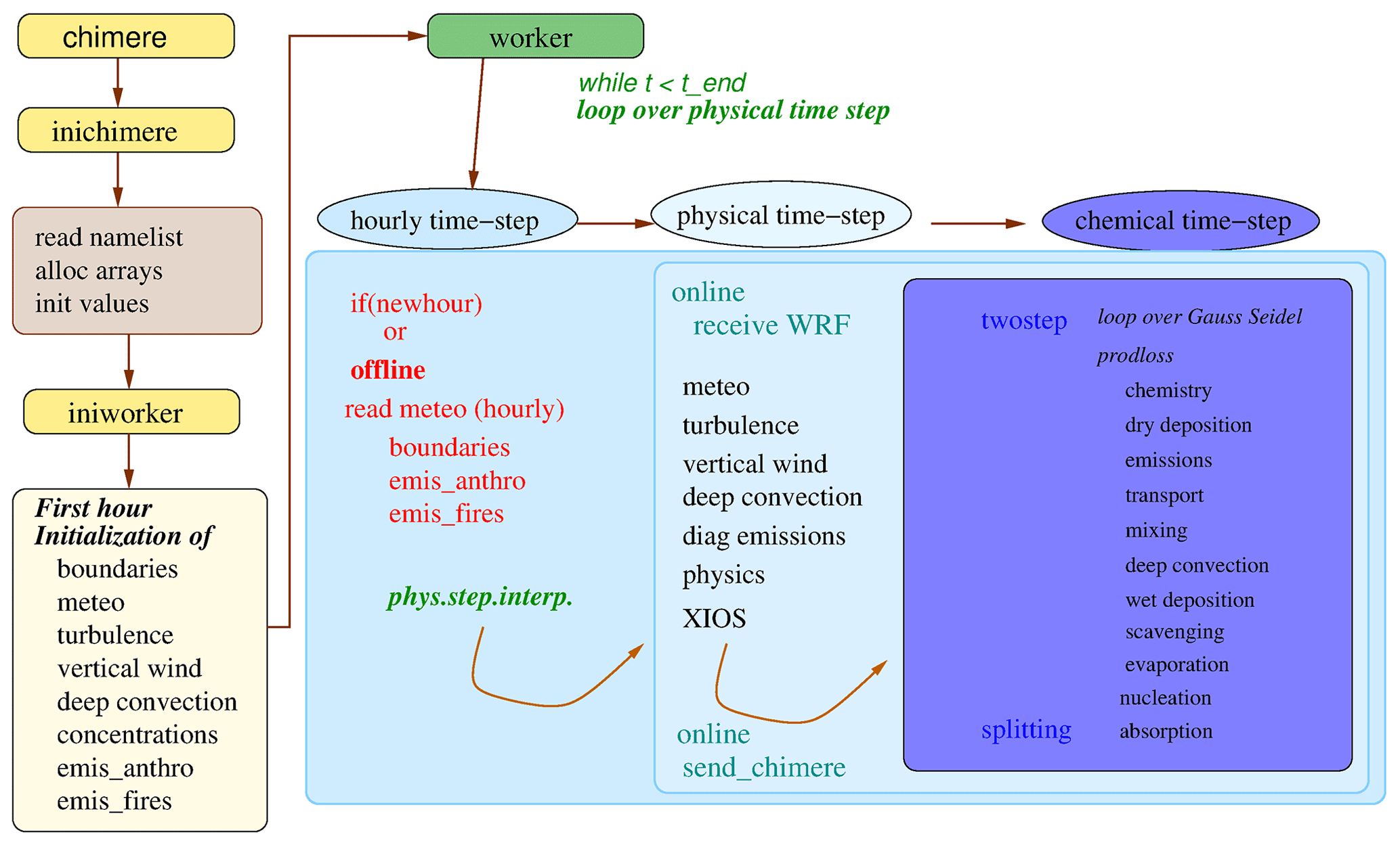
Figure 1Organization chart of CHIMERE v2023r1. The first yellow boxes present the initialization phase: static namelist and initial values are selected only on one processor (inichimere). Second, on all processors, the main fields are initialized for the first hour: boundary conditions, meteorology and concentrations of all chemical species (iniworker). Finally, the main temporal loop is performed (worker). It includes an hourly time step (in offline mode), then a physical time step, and then a chemical time step. Depending on the mode (offline or online), some exchanges are performed between the WRF model and the CHIMERE model.
Figure 1 presents the organization chart of this model version. The main program is called chimere. This program mainly manages three different blocks. First, the inichimere routine is called and is dedicated to the initialization of each module: reading input parameters (namelists or aerosol size distribution and list of chemical species, among others) and computing fixed parameters and array allocations. Depending on the processes requested by the user, modules are initialized or not; this way we prevent unnecessary file reading or memory burden. In the case of online coupling, an additional namelist for OASIS is read. Second, another initialization part has to be done in the iniworker routine. This is performed only for the first simulated hour in order to obtain values at zero time for all input variables: meteorology, turbulence, anthropogenic and fire emissions (depending on input databases), and boundary conditions. Third, the loop over time starts and is managed for each processor in the worker routine. This loop is performed at the physical time step, a sub-hourly division depending on the domain cell sizes. Depending on whether the simulation is offline (no feedback between chemistry and weather) or online (in blue), meteorological fields are read (hourly; in red) or received from WRF (physical time step; in blue). In the case of it being online, the concentrations are sent to WRF to take into account direct and indirect effects for the next physical time step. If offline, if the time step coincides with an entire hour, the hourly boundary conditions and anthropogenic and fire emissions are updated. For these hourly fields, a linear time interpolation is performed to retrieve information at the corresponding physical time step. Next, all processes related to the physical time step are performed: emissions, resuspension, aerosol physics, mixing, photolysis, deposition and chemical rates. Once we have all the necessary information, a loop is performed at the chemical time step. Two chemical solvers are available: twostep and splitting, as already explained in Menut et al. (2021a). For example, in twostep, the first step is performed, and then an additional loop is performed with Gauss–Seidel iterations for the second step. Finally, the newly implemented XIOS routine is called to write the results on the disc.
The model has thus three main steps: initialization of modules, initialization of first table values at zero time and time integration. The time integration contains three levels: (i) a sub-hourly physical time step, mainly depending on the grid size for meteorological variable accuracy; (ii) a chemical time step depending on the Courant–Friedrichs–Lewy (CFL) condition (Courant et al., 1952); and (iii) the Gauss–Seidel iterations (at least two are recommended).
2.2 XIOS I/O management library
Version 2 of XIOS (XIOS2) has been implemented in CHIMERE. XIOS (XML-IO-Server) is an open-source C++ library dedicated to I/O management that is usable in conjunction with numerical models written in Fortran/C/C++ (XIOS, 2023). It is a powerful tool for both output history file management and spatial and temporal post-processing of data at runtime. XIOS was developed with several goals in mind: (i) simplifying the I/O management inside the source code by reducing the number of calls needed to send a variable to be written; (ii) offering flexibility to the user without having to make modifications inside the source code; and (iii) making writing and computing happen simultaneously using asynchronous calls, meaning that the writing will not slow down the computation. XIOS manages to achieve these goals by setting up servers and clients; one or several CPUs can be dedicated to XIOS servers, which manage I/O processes exclusively. These servers receive asynchronous data from what are called clients (here the chimere ranks) and write them into one or multiple files; they can also manage any additional temporal or spatial post-processing requested by the user. XIOS has been implemented and evaluated in several models. Among many others, Institut Pierre-Simon Laplace (IPSL) Earth system models use XIOS exclusively (Boucher et al., 2020).
File and variable management is done by XML files. For standard use of the model, all necessary files, variables and parameters have been prepared in standard XML files, and the use of XIOS is transparent for the user. However, one of the perks of using XIOS is the flexibility it offers the users. This means that the user can create almost any combination of output files they want by adding or removing species or dimensions. Indeed, the XML files can be modified or new ones can be created at any time by the user without the need to recompile the model or, largely, even code in the model. Here, we list some common tasks that XIOS can perform:
-
Hourly minima, maxima or averages of a particular species can be processed by XIOS and written to the disc without adding more computation time. For example, maxima can be useful for calculating air quality threshold exceedances.
-
Species can be written only for a specific part of the domain (like a sounding or a subdomain) or a specific layer (the surface, for instance).
-
Arithmetic operations can be performed to sum up variables in a chosen dimension.
-
The user is completely free to define an output file only with the variables that are important for their specific usage.
Examples of such personalized cases have been provided in the code. It is important to keep in mind that customizing an XML file to create personalized XIOS output files is not limited to the examples provided by the development team, and each user can create output files that correspond to their specific needs.
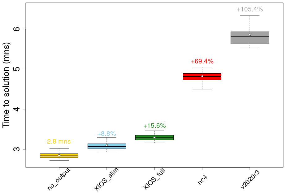
Figure 2Runtime comparison between several I/O options implemented in the model. Each boxplot contains thirty 1 d simulations, and the black line on each boxplot shows the average for each configuration. Five options are shown – no_output: model does not write any output files; XIOS_slim: an example of a personalized XIOS output; XIOS_full: the standard output files of the model written with XIOS; nc4: the standard output files of the model written with the standard I/O module in the model; and v2020r3: the previous distributed model version. The additional time (in %) is shown above each boxplot. For the no_output case, the average time in minutes is shown.
The performance of XIOS and the standard I/O system using netCDF 4 in parallel in the model (called nc4 hereafter) has been compared extensively. Figure 2 shows runtime comparisons of thirty 1 d simulations in different configurations. Two configurations of XIOS are shown here: the standard configurations that replicates the nc4 output files to the letter (called XIOS_full) and an example of a personalized configuration which only writes a list of species necessary for the usage in mind (called XIOS_slim). These are compared to the model runtime when it does not write any output, which can be considered the pure calculation time of the model (including reading of input data). The figure shows that using XIOS offers an important reduction in the runtime of the model, adding only 8.8 % and 15.6 % to the runtime for the XIOS_slim and the XIOS_full configurations, respectively. Compared to the added 69.4 % computation time in the case of the standard I/O module, XIOS offers a good performance increase in the model. Finer tuning of the performance is also possible by adapting the number of I/O servers or the size of buffers. Finally, this new model version is compared to the previous one, the distributed v2020r3 version: with a time increase of +105.4 %, the new model version is 2 times faster than the previous one.
2.3 Update of the user parameter namelist
The CHIMERE parameter file chimere.par was updated in order to remove some unused parameters and to add novelties. The complete list of parameters is presented in the model documentation (https://www.lmd.polytechnique.fr/chimere/docs/CHIMEREdoc_v2023.pdf, last access: 9 July 2024) for all possible flags. In this section, only the new flags corresponding to new functionalities are explained.
-
forecast. The forecast is re-activated in this model version. It is mainly the way to manage the WRF files when preparing the meteorology.
-
nproc_chimere, nproc_wrf and nproc_xios. These options are for the management of the simulation as a function of the available processors, for CHIMERE, WRF and XIOS, respectively. Obviously, the total of the three must be less than or equal to the total number of the available processors on the user's computer. For CHIMERE and WRF, the number of processors corresponds to the number of subdomains for the parallel computation. If you are offline, the number of subdomains is calculated for CHIMERE only. For example, in online mode, for a cluster core of 64 processors (classical configuration), it is recommended to select 15 for WRF, 45 for CHIMERE and 2 for XIOS.
-
ifire2dust, ifire2lai and ifire2drydep. These options concern the effect of the fires on other processes. This takes into account the possible changes in soil erodibility and surface wind speed and the leaf area index (LAI) for the biogenic emissions and for the dry deposition of gaseous species following Menut et al. (2023).
-
ilai. This option is used to select the LAI database between ilai = MOD (MODIS; Yuan et al., 2011) and ilai = COP (Copernicus; Fuster et al., 2020).
-
ip_ragweed. It checks whether the ragweed pollen calculation is activated (1) or not (0). Three schemes are available for this pollen type: (1) for the Sofiev et al. (2013) scheme, (2) for the Efstathiou et al. (2011) scheme, and (3) for the Menut et al. (2021b) scheme. Calculations are explained in Sect. 6.2.
-
ip_birch, ip_grass, ip_alder and ip_olive. These are dedicated to activating (1) or not activating (0) the pollen emissions for birch, grass, alder and olive, respectively.
-
ipolresus. This option activates the resuspension only for pollen.
-
pollendir. This option indicates the directory where all pollen databases are stored. For this model version, and with no other available dataset, pollen forcing data are available only over western Europe.
-
gtrc and ptrc. These activate the gaseous and aerosol tracers, respectively. It is necessary to complete two ASCII files (see Sect. 3.2): TRACERS_GAS.data and TRACERS_PART.data.
-
dgrb. This is the directory where the global meteorological files in GRIB format are stored (ECMWF or NCEP).
-
geodata. This is the directory of surface input data for the WRF Pre-Processing System (WPS). In this version, WPS (from WRF) is distributed since the domain file used by CHIMERE is the geog file of WRF. This avoids some interpolations of meteorological fields and then reduces errors in the meteorology and speeds up the model.
-
dmin and dmax. These options enable the definition of the limits of the aerosol size distribution. dmin and dmax are the size of the first interval of the first bin and the last interval of the last bin, respectively. These limits are the same for all aerosols. Values of 0.01 and 40 µm are recommended.
-
iforcut. If this flag is equal to 1, the calculation of the size distribution is forced to have retained the diameter of 2.5 and 10 µm as the cutoff.
-
timeverb. This flag manages some text printed on the screen, providing the time step in each module of the model. It is mainly useful to developers to see if new calculations have an important numerical cost.
-
AODPerSpecies. The aerosol optical depth is the outputted aerosol species per species.
The chemical module SSH-aerosol (Sartelet et al., 2020) is now compatible with CHIMERE to represent aerosol dynamics. SSH-aerosol is distributed independently of the CHIMERE model, and it will evolve in the next few years. It means that in order to be able to use this specific option, the user needs to download the SSH-aerosol module and compile it independently of all CHIMERE programs. For this, a specific script is available in the CHIMERE main folder to download SSH-aerosol. In the CHIMERE namelist, the use of SSH-aerosol is activated when values of soatyp are h2o or h2or. A specific namelist for SSH-aerosol is proposed in the namelist_ssh folder, and it can be adapted by the user according to the level of complexity suitable for computing aerosol dynamics. Note that, in this version, the SSH-aerosol package is currently only compatible with the operator splitting option and not with the twostep option. For consistency between the secondary organic aerosol (SOA) compounds in gas and particle phases, the MELCHIOR 2 chemical mechanism is recommended.
3.1 Changes in the advection formulation
The advection schemes have been corrected and updated, and new schemes were added as a user's choice. The user can select different schemes for the horizontal and the vertical transport, the two being calculated separately.
In the vertical direction, the Després and Lagoutière (1999) scheme has been implemented. As described in Lachatre et al. (2020), two options are now available for the representation of vertical velocity: diagnose it either from the horizontal wind components, as it was historically done in CHIMERE, or using the vertical wind speed provided by the meteorological model. Lachatre et al. (2022) have shown that reducing numerical diffusion using the Després and Lagoutière (1999) advection scheme and using the vertical wind speed, w, from the meteorological model (is_diagwinw = .false. in chimere.par) also modifies the chemical processes in thin plumes; due to the nonlinearity of tropospheric chemistry, diluting a plume over a larger volume changes not only its distribution, but also the kinetics and relative importance of the chemical processes.
For horizontal advection, five different schemes are available: (1) the simple first-order advection scheme of Godunov and Bohachevsky (1959). It is the fastest scheme and may be used in the case of low resolution or forecast when results are expected soon. However, it is also diffusive and is not recommended in the case of thin plume studies. (2) The Van Leer scheme is fast and accurate (Van Leer, 1977). (3) The parabolic piecewise method (PPM) scheme (Colella and Woodward, 1984) has been revised and is now faster than the previous implementation. (4) The Walcek (2000) advection scheme has been implemented, and, finally, (5) the PPM+W advection scheme, a combination of the PPM and Walcek schemes, has been implemented (Mailler et al., 2023c). In an academic framework, Mailler et al. (2023c) have shown that the PPM+W performs best among these schemes in terms of accuracy, while the Van Leer and Walcek schemes are computationally cheaper. The PPM+W scheme has a computational cost similar to PPM.
3.2 Changes in tracer management
The introduction of “tracer” emissions inside model simulations including other (realistic) emissions or not is a possibility offered by the CHIMERE model. In CHIMERE, the word tracer does not necessarily imply that the species is inert chemically. The emitted species can be chemically either inert (as in Lachatre et al., 2020) or active (as in Lachatre et al., 2022) as soon as the emission occurs over a finite number of horizontal points (but possibly spread in the z direction). The user can specify the vertical repartition of tracer emissions and their evolution in time. This framework is well suited not only to include emissions due to volcanic eruptions or industrial accidents, for example (e.g. Lachatre et al., 2022), but also to study the behaviour and motion of air masses to and from key areas such as cities or mountain valleys (Lapere et al., 2023; Deroubaix et al., 2019). Lachatre et al. (2022) show an example of a real species (SO2) emitted as a tracer over a specific point, along with its normal surfacic anthropogenic emissions from emiSURF.
In the new version of the CHIMERE model, gas and/or particulate tracers are set in two distinct input files (TRACERS_GAS.data and TRACERS_PART.data). The users decide to activate gas tracers or not by acting on two distinct parameters in the chimere.par file:
-
gtrc. It is to be set to 1 (resp. 0) to activate (resp. deactivate) gas tracers.
-
ptrc. It is to be set to 1 (resp. 0) to activate (resp. deactivate) particulate tracers.
Compared to earlier model versions, the new model version permits more flexibility and user control for particulate tracer emissions: for each tracer emission event, up to three different emission modes can be specified (from the median diameter and the multiplicative spread of the log-normal distribution), independently from the modes defined for anthropogenic emissions. In the TRACERS_PART.data, for each tracer emission, the user can define the following parameters:
-
longitude and latitude of the emission point
-
onset date and termination date of emission in the YYYYMMDDHH format (in v2023r1, the emission duration must be an entire number of hours and at least 1 h)
-
emitted tracer mass
-
minimum and maximum altitude of emission (the tracer mass will be distributed evenly between these two altitudes)
-
f1, f2 and f3 – fraction of tracer mass in the first, second and third size mode, respectively (the user must check that )
-
D1, D2 and D3 – mass median diameter of the first, second and third size mode, respectively, for the emission.
-
σ1, σ2 and σ3 – geometric standard deviation of the first, second and third size mode, respectively, for the emission (σi>1)
The proportion of tracer mass between diameters Dm and DM>Dm is
These three emitted modes are then distributed into the nbins size bins for chemistry and transport, as described in Menut et al. (2013).
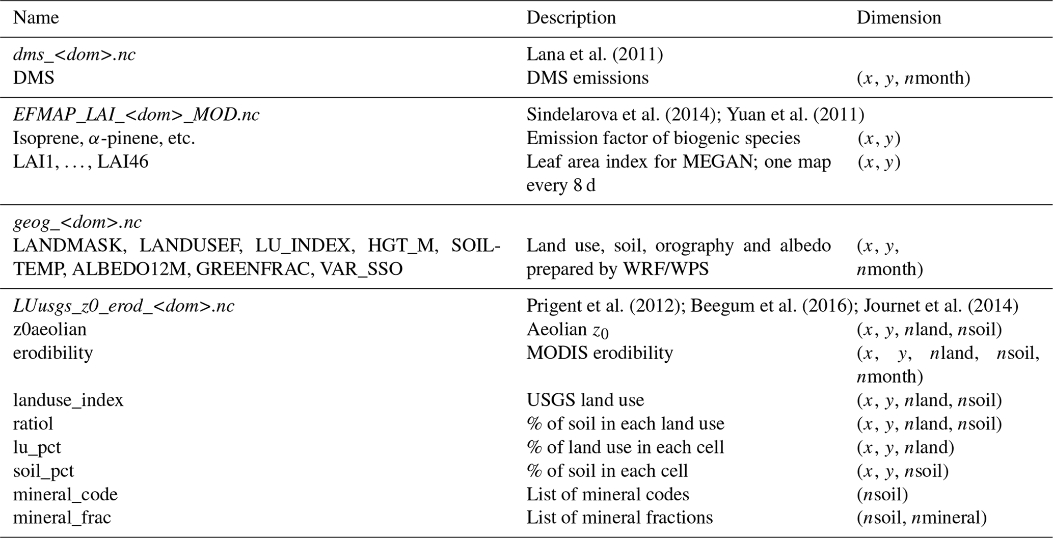
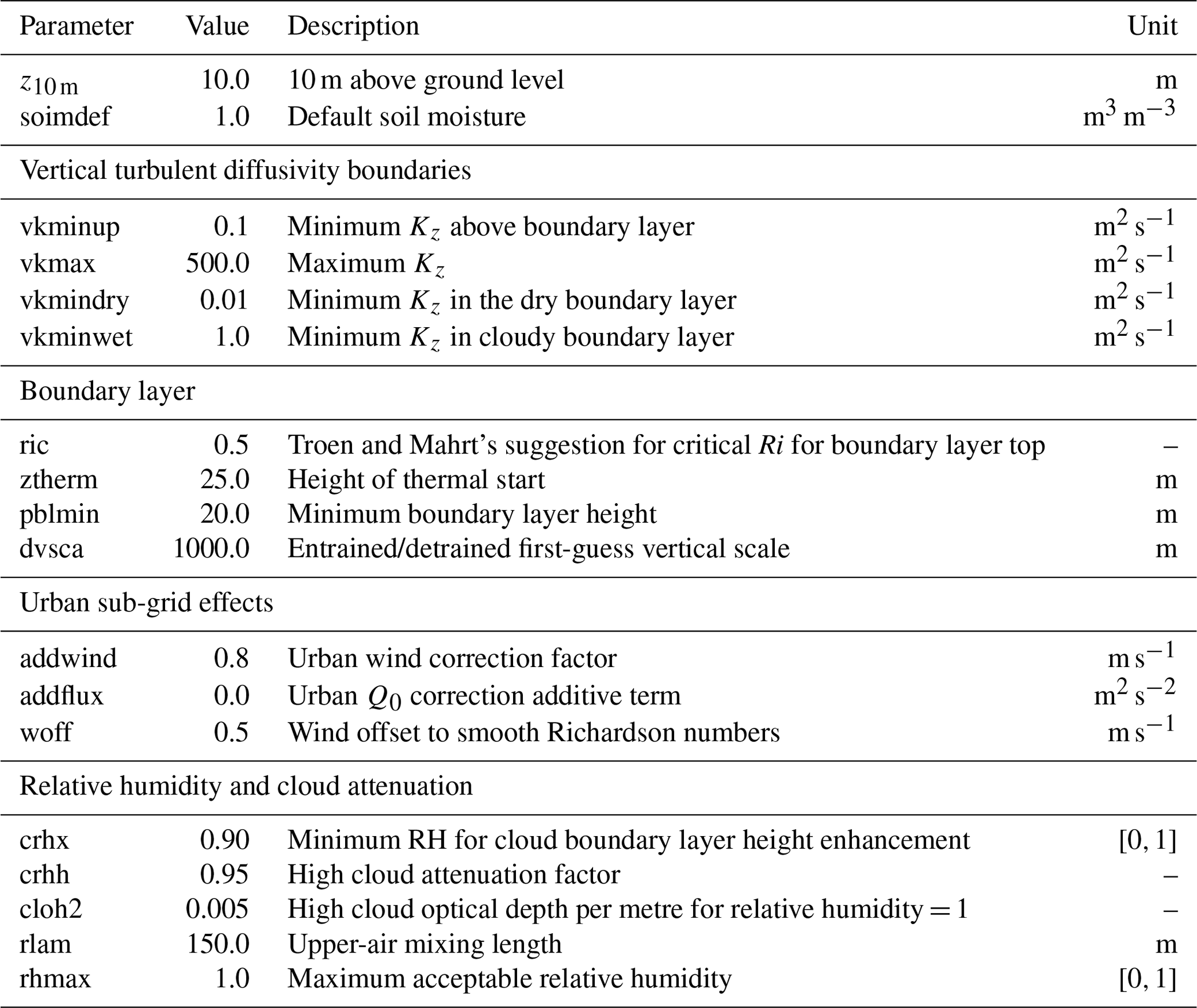
The pre-processing for the CHIMERE-specific nine classes of land use was removed in this version. We made the choice to directly use the land use generated by the WRF Pre-Processing System (WPS) and its output geog file. This permits it (i) to be faster to prepare in pre-processing; (ii) to be consistent with the meteorology when the two models, WRF and CHIMERE, are coupled; and (iii) to be consistent with the sub-grid-scale approach of the mineral dust emissions. Changing the land use classes imposed an update of the surface information required for turbulence, resuspension, albedo calculations and dry deposition. The surface information required for a simulation is presented in Table 1.
Lana et al. (2011)Sindelarova et al. (2014); Yuan et al. (2011)Prigent et al. (2012); Beegum et al. (2016); Journet et al. (2014)Table 1Files and variables required to initiate a CHIMERE simulation.
The use of a new tabulated dynamical roughness is done using the values proposed by the WRF model, which are already fitted for the United States Geological Survey (USGS) land use. The seasonality is considered using the WRF green vegetation fraction (GVF) as a proxy, with the following equation:
In Table A1, the last z0 m value, representative of water surface, is here set to zero but later calculated using the Charnock scheme (Charnock, 1955) (see Sect. 5.2 for the detailed calculation). Following the same process, the albedo values are tabulated and are presented in Table A2. It impacts the calculation of the resuspension: with the new land use, the resuspension is applied for all cell percentages related to urban and agricultural areas following USGS land use classification. It also impacts the dry deposition, and a new correspondence matrix was defined between the European Monitoring and Evaluation Programme (EMEP) (Emberson et al., 2001) and the USGS land use classes.
All calculations dedicated to turbulence were grouped into a single Fortran module. Some parameterizations were updated at the same time. Compared to CHIMERE v2020r1, this new module includes the following changes:
-
The roughness length over the sea, z0, is not tabulated but calculated using the Charnock equation (Charnock, 1955).
-
The parameterization of the surface sensible heat flux, Q0, and the aerodynamic resistance, ra, were upgraded to a more recent scheme. For ra, its calculation is now on the CHIMERE vertical levels and not on the meteorological vertical grid.
-
The calculation of turbulent parameters is now on a loop to ensure consistency between all variables (it includes Monin–Obukhov length calculation).
-
It is now possible to diagnose the 10 m wind speed , the one from WRF that is dependent on the boundary layer height scheme and not always satisfying.
5.1 Variables to read or diagnose
In the CHIMERE model, many boundary-layer-related variables can be diagnosed. However, if the meteorological driver model provides some of them, they could be read directly and then used to diagnose the missing ones. The variables that can be read are selected in the chimere.par file and are the following:
-
idiagblh. These variables use boundary layer height of the weather driver (idiagblh = 0) or diagnose it (idiagblh = 1) following Troen and Mahrt (1986).
-
idiagflux. These variables use the surface turbulent characteristics as the friction velocity u* and the surface sensible heat flux Q0 of the weather driver (idiagflux = 0) or diagnose it (idiagflux = 1) following Troen and Mahrt (1986).
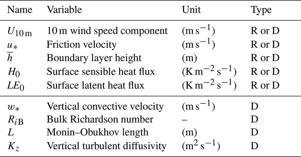
Depending on this choice, the list of variables that can be read or diagnosed and those that can only be diagnosed is presented in Table 2.
Table 2List of variables required to describe the turbulence in and above the boundary layer. R stands for read and D for diagnostic.
For all calculations, several constants are defined in the code. They can be modified by the user, but it is not really recommended. These constant values are listed in Table 3.
Table 3Constant values used for the calculation of additional parameters in the routine calc_turb.
5.2 Diagnostic of meteorological variables
Before starting the calculation of the turbulent parameters, it is necessary to estimate some other variables. A specific order is required, with some variables being estimated using other variables.
First, the surface pressure, Psurf, is simply diagnosed using the pressure values at the two first model levels:
The same calculation is applied to estimate the surface values of specific humidity, cloud liquid content, ice content and rain. The surface values of wind components are set to zero. The total amount of water in the atmosphere is
where cliq, cice and rain are the cloud, ice and rainwater mixing ratio (kg kg−1). The potential temperature θ is calculated as
with T being the air temperature (K), P0=100 000 Pa the reference pressure, Ra=287.04 J K−1 kg−1 the specific gas constant for dry air and Cp=1005 J K−1 kg−1 the specific heat capacity of air. Note that the ratio is also noted and used as γ=0.2857. The virtual potential temperature, θv, is the equivalent of θ but accounting for dry and humid air as
The wind speed module, (m s−1), is expressed as
Air density is calculated (in molecules m−3) as
with mol−1 and Mair=29 g mol−1 the molar mass of air.
For the calculation of relative humidity (RH), the partial pressure of water vapour, e* (Pa), is first estimated following Tetens' formula (Tetens, 1930) as
with T0=273.15 K. The dew point (in g g−1) is deduced as
Finally, the relative humidity is calculated as
with q being the specific humidity. The relative humidity is protected against extreme values and bounded to the rhmax constant value defined in Table 3.
One key point for turbulence parameterizations is to diagnose the near-surface virtual potential temperature, here noted as θv,0. To access this value, we extrapolate the vertical temperature profile using the 2 m temperature, T2 m, and the temperature at the first model vertical level, T1, to obtain T0. The following expression is used:
Over sea, it is common to use the Charnock equation to estimate the momentum roughness length, which is dependent on the sea surface and the wave height:
where αc is a constant (αc≈0.015). Pena and Gryning (2008) note that this constant could range between 0.008 and 0.06 depending on the study. An iterative approach is necessary to quantify the roughness length depending on the friction velocity and vice versa of the two. Fortunately, Hersbach (2011) proposes an efficient fit to estimate z0 without knowledge of u*:
with and . The two parameters expressed that z0 depends on kinematic viscosity, ν, for light wind and on the Charnock relation for strong wind. They are estimated with
with k=0.41 being the von Kármán constant, m2 s−1 the kinematic viscosity, un the wind speed at height z (here z=10 m), αM=0.11 and αch=0.018 the Charnock constant. However, this constant varies following studies and ways to determine it as, for example, explained in Feng et al. (2021). This roughness length calculated for three different Charnock constants is displayed in Fig. 3.
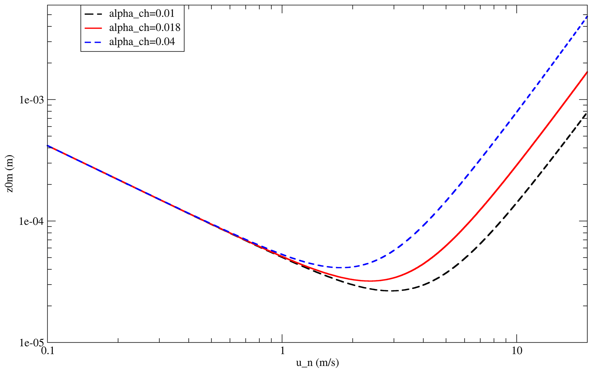
Figure 3Roughness length over water surfaces calculated for three different Charnock constants.
5.3 Optical depth above model top
In order to have the optical thickness due to clouds for the full tropospheric column, an optical depth is estimated above the CHIMERE domain top using the meteorological model data. It is generally possible since the CHIMERE model currently has a model top around 200 hPa (user's choice), while the meteorological model has a model top around 50 hPa. For the atmospheric column in CHIMERE, the Fast-JX module calculates the cloud optical depth (COD) directly. The top level of CHIMERE, ptopchimere, is first estimated in the meteorological model grid. The following equation is then used:
where 0.95 is the value of high cloud attenuation and is the high cloud optical depth for RH = 1 (in m−1). ptopmeteo is the pressure of the top level of the meteorological model. Finally, the attenuation due to cloud above the model top is estimated using the following empirical formula:
5.4 Urban correction
A simple urban correction is available in the model. This is very simple and only implemented to retrieve some observed trends: lower surface wind speed and higher surface sensible heat flux. This option may be activated in the chimere.par parameter file by changing the urbancorr flag. This activation induces a slight change for the wind speed in the surface layer (from ground to surface layer height) and Q0, the surface sensible heat flux, only over urbanized areas as
The factor for the wind speed is equal to the proportion of urban surface in the cell multiplied by a factor defined in the module calc_turb.F90 as a parameter, factU. A standard default value is 0.8. The change for Q0 is an additional flux called addQ0 and equal to 30 W m−2. These values may be changed directly in the model code. Note that this correction is applied to the wind profile, (u,v), before the diagnostic of turbulent fluxes and after the diagnostic of Q0. The values correspond to a concatenation of wind and temperature observations found in numerous publications on urban meteorology, such as Oke (1982), Calbo et al. (1998) and Arnfield (2003).
5.5 Diagnostic of turbulent variables
It is possible to directly use the turbulent variables calculated by the meteorological forcing model. For that, two conditions have to be fulfilled: (i) the flag idiagflux = 1 in chimere.par and (ii) the corresponding variables, friction velocity, u*, and surface sensible heat flux, Q0, must be available in the meteorological model outputs. If these two conditions are not reached together, these variables have to be diagnosed, with each variable being dependent on the others. Due to these dependencies, it is an iterative process.
5.5.1 The Richardson number
First, a calculation of the surface layer turbulent variables must be done. It is necessary to calculate the stability of the atmosphere. Following the scheme of Jiménez et al. (2012), the bulk Richardson number is calculated as follows:
with θvg and θva (K) being the virtual potential temperature at ground and first model levels, respectively. The first vertical model level is at height z. g is the acceleration of gravity. U is the mean wind speed at altitude z. To avoid values of Rib that are too large and unrealistic, a minimum value of U=0.1 m s−1 is forced.
The Monin–Obukhov length, L, is iteratively estimated using the first-guess value of Rib and the following equation:
with ΨT being equal to
where z0 m is the momentum roughness length and is tabulated. For the heat roughness length, several formulations and uses exist. For example, Beljaars and Holtslag (1991) use . In Jiménez et al. (2012), all equations use only z0 without distinction between momentum and heat. We thus apply the relation z0h=z0m here because the use of a lower z0h gives too low of a surface sensible heat flux. The stability functions (for momentum) and (for heat) are calculated using the modified formulation of Jiménez et al. (2012).
-
If Rib>0 (nocturnal stable boundary layer), then
with a=6.1, b=2.5, c=5.3 and d=1.1.
-
If Rib≤0 (free unstable conditions), then
where represents the convective contribution as
with . αm=10 and αh=34, after Grachev et al. (2000). represents the Kansas-type contribution as initially proposed by Paulson (1970).
with and γ=16.
5.5.2 The friction velocity (u*)
The friction velocity, u*, and the potential temperature scale, θ*, are calculated as follows (Beljaars and Holtslag, 1991):
Note that we also added the correction term here, with in place of z. For the first iteration, we can calculate u* and θ* under neutral conditions, considering ψm and ψh are equal to unity. The Monin–Obukhov length, L, is then updated as
The iterative algorithm may be summarized as follows:
- 1.
Rib is calculated using the meteorological variables in Eq. (20).
- 2.
L is estimated using Eq. (21) and considering neutral conditions to have .
- 3.
A loop is then performed with the
- (a)
calculation of ψm and ψh with the updated value,
- (b)
calculation of u* and θ* using the updated ψm and ψh, and
- (c)
calculation of L using the updated u* and θ*.
- (a)
The iterations stop when two successive values of L are lower than a pre-defined threshold. Here, we use ΔL=0.1. After several tests, the convergence is generally reached after four iterations.
The 10 m wind speed is then diagnosed by
5.5.3 The surface heat fluxes
The surface heat fluxes are not always provided in forcing models. But we need this quantity to evaluate w* and . For its quantification, there are two ways. First, we have the information about the sensible H (W m−2) and latent LE (W m−2) turbulent fluxes (the “eddy fluxes”). We can thus estimate the fluxes close to the surface as
with R being 287.04 J K−1 kg−1, Cp the specific heat capacity (Cp=1005 J K−1 kg−1) and Lv the latent heat of vaporization ( J kg−1). Hurb is an additional surface sensible heat flux that represents an urban contribution and is chosen to be Hurb=0 by default. A value of Hurb=30 W m−2 is often used in regional or urban modelling. The total (heat + latent) surface flux, Q0, is then estimated as
Second, if we have no information, we use the previous parameterized values of u* and θ*. Q0 is estimated to be
5.5.4 The boundary layer height
If the boundary layer height () is available in the meteorological model and if it is the user's choice, the variable is just read and not calculated. If the user prefers to have a diagnostic made in CHIMERE, the calculation is done as follows. To select the use of the meteorological model, the following two conditions must be reached: (i) the boundary layer height, , must be available in the meteorological model outputs, and (ii) the flag idiagblh must be 0 in chimere.par.
In the case of diagnostics, the following calculation is performed. Formulations are different depending on the atmospheric static stability. When stable, i.e. when L>0, is estimated to be the altitude when the Richardson number reaches a critical number, here chosen to be Ric=0.5, following Troen and Mahrt (1986). Under unstable situations (i.e. convective), is estimated using a convectively based boundary layer height calculation. This is based on a simplified and diagnostic version of the approach of Cheinet and Teixeira (2003), which consists of the resolution of the (dry) thermal plume equation with diffusion. The in-plume vertical velocity and buoyancy equations are solved, and the boundary layer top is taken to be the height where calculated vertical velocity vanishes. Thermals are initiated with a non-zero vertical velocity and potential temperature departure, depending on the turbulence similarity parameters in the surface layer. The two formulations are used, and the maximum of the two diagnosed values is retained.
5.5.5 The free convection velocity scale (w*) and the aerodynamical resistance (ra)
Now that we have the boundary layer height, , it is possible to more properly estimate the free convection velocity scale, w*:
where is the convective boundary layer height and the mean virtual potential temperature at the first model vertical level. For the aerodynamical resistance, we use the Bruin and Holtslag (1982) equation:
with U being the wind speed at height z (in our case, the first vertical model level). Note that Bruin and Holtslag (1982) use a fit with the momentum roughness length z0 m, while the usual expression of ra uses the heat roughness length. This fit replaces the regular expression of the aerodynamical resistance (Beljaars and Viterbo, 1994) by
5.5.6 Momentum vertical turbulent diffusivity (Kz)
The momentum turbulent diffusivity, Kz (m2 s−1), has different formulations depending on the period of the day (stable or unstable conditions) and the altitude (surface layer, mixed layer or free troposphere).
In the surface layer, when conditions are stable, the turbulence is the most difficult to diagnose, with the variances of meteorological variables being very small. Troen and Mahrt (1986) remind us that when the surface layer is considered to be in equilibrium, then the parameterization of Louis (1979) is used. In the mixed layer, Kz is calculated following the parameterization of Troen and Mahrt (1986) without the counter-gradient term by
where k=0.41 is the von Kármán constant, z the altitude, the boundary layer height and ws a vertical velocity scale. Note that the formulation of Eq. (1) in Troen and Mahrt (1986) is false. The calculation of ws depends on the atmospheric stability. For the stable case, the following applies:
On the other hand, for the unstable case, the following applies:
The constant ϵ is determined to be 0.1 in Troen and Mahrt (1986). For the model, this value is defined as to ensure a robust calculation in the first few vertical model levels. To avoid numerical problems, values of Kz are bound using pre-defined constant values, as explained in Table 3.
Above the boundary layer and in the presence of clouds, an additional diffusivity is added. This diffusivity is estimated if the relative humidity is larger than 0.9. For each model vertical level, a new vertical diffusivity, Kz, is estimated. The formulation is inspired by the Betts et al. (1995) study and the implementation of the turbulence scheme in the NCEP operational Medium-Range Forecast (MRF) model. The concept is based on the Louis (1979) formulation, defining stability function.
The vertical diffusion coefficient, (as a function of altitude z and for momentum m and heat h), is expressed here as
where Ri is the local gradient Richardson number, U the wind speed module, z the altitude, fm,h the stability function for momentum and heat, and l the mixing length diagnosed as
with k being the von Kármán constant and λc the asymptotic length scale, with λc=150 m (but 250 m in Betts et al., 1995). The stability functions, fm and fm,h, are estimated to be
with Cm=1.746 and Ch=1.286.
Emissions are the main chemical forcings of the model. In parallel with the development of the CHIMERE model itself, the various emissions taken into account are also updated between two versions. This section therefore presents emissions newly taken into account as well as updated and improved ones.
6.1 Changes in anthropogenic emissions
The management of the anthropogenic emissions has changed in this version of the model. The goal is to have fewer files to manage, which is a sore point of supercomputers. The new format corresponds to one file per day of the week, so seven files per month. Indeed, we have temporal data to differentiate the months of the year, the days of the week in a month and the 24 h of a day.
All chemical emitted species are grouped together in each file (before it was one file per species). For each species, the resolution is hourly and the fluxes are projected on the horizontal grid of the model. Using the provided emiSURF program, the user can also choose to differentiate their emission fluxes by activity sector according to the GNFR nomenclature. This differentiation will then be necessary in the case of simulations using the sub-grid variability option.
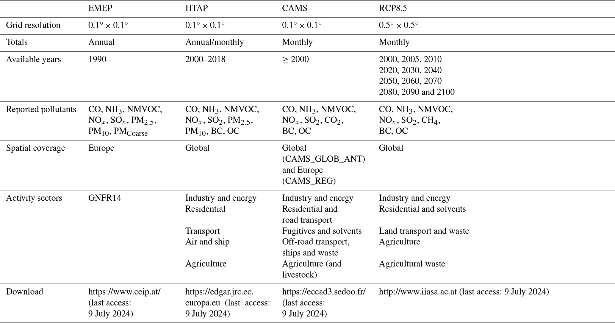
Finally, the user is encouraged to use the emiSURF model (described in Mailler et al., 2017) developed by the CHIMERE model team. This model is able to ingest multiple input databases, as described in Table 4. In its latest version (v2023r1), emiSURF takes into account the most recent time factor data (Guevara et al., 2021; Crippa et al., 2020).
Table 4The different anthropogenic emission inventories processed by the emiSURF model. NMVOC: non-methane organic volatile compound, BC: black carbon, OC: organic carbon.
6.2 Implementation of pollen emissions
Pollen emissions were taken into account in a parallel version of CHIMERE operated by INERIS for the Copernicus daily forecast over Europe. The code was cleaned up and is now implemented in the official CHIMERE version. It means that from now on, pollen emission, transport and deposition will always be available in CHIMERE. This development comes in addition to the simulation of gases and aerosols: pollens are inert and there are no interactions with other pollutants. Model scores are therefore not modified if pollens are calculated. Additional details about this calculation in CHIMERE are presented in Sofiev et al. (2015) (for birch) and Menut et al. (2021b) (for ragweed).
6.2.1 The pollen grain specifics
Pollen grains are very different from the usual atmospheric aerosols. Regarding their transport, Sofiev et al. (2006) showed that they can be transported together with air masses and may be mixed due to small turbulent eddies. In this model version, five different pollen species were implemented: birch, olive, ragweed, grass and alder. The pollen density depends on each species and varies between 800 and 1200 kg m−3, which yields the sedimentation velocity of 1.2–1.3 cm s−1. The main dry deposition process for pollens is gravitational settling, and they can be washed out by rains. For pollen, only the “big” mode of the aerosol is designed. The pollen species are considered non-chemically reactive. Optical properties are prescribed for short-wave and long-wave wavelengths.
6.2.2 Main principle of emissions for birch, grass and olive
To calculate pollen emissions, several surface databases are needed. In this model version, the databases are limited to western Europe. Three parameters are needed for each species: the surface fraction, the heat sum threshold and a scale factor. For the grass pollen, the data come from the SILAM model (Sofiev et al., 2006). Some additional information is provided: the mean diameter, Dp=32 µm; the density, 800 kg m−3; and the height above surface, h=1 m. Note also that there is no time dependency in this database. It is probably to improve later since the ragweed locations increase every year in Europe (Schaffner et al., 2020).
The pollen emission modelling is challenging because it requires fair knowledge of plant distribution and phenology and adequate assumptions regarding the sensitivity to meteorological factors, such as humidity, temperature, wind speed and turbulence. Unlike industrial pollutants or mineral aerosols, pollen emissions depend on not only the instantaneous meteorological conditions, but also the conditions during the pollen maturation within the plants before the pollination starts: it means that an accurate simulation is required to start several months before the targeted period. For all species, emissions schemes have the same basis:
where D(x,y) is the ragweed density distribution in number of individual plants per square metre. is the annual production in grains per individual plant. is the phenology factor (in s−1), considering its yearly integrated value is unity. This factor represents the knowledge of the start and end dates of the pollen season as well as the shape of these potential emissions. is the daily or sub-daily weather-dependent release of pollen grains in the atmosphere which depends on the hourly (or daily) meteorological variables. is unitless. These different terms correspond to two different temporal scales: D(x,y), and represent “annual” information and represents “short-term” information for which we want to evaluate correlation with the meteorological variables.
To calculate these terms, we used the scheme of Prank et al. (2013) (referred to as P2013 hereafter). It is the scheme used in SILAM (Sofiev et al., 2013). Originally developed for birch pollen, it was adapted to ragweed by Prank et al. (2013). It is also used for olive, grass and alder. This SILAM version is directly implemented in CHIMERE and used without any changes. This scheme is based on a double-heat-sum concept (Linkosalo et al., 2010). The temperature accumulates from the 60th day of the year (29 February or 1 March), and when the accumulated heat sum reaches the first threshold, the flowering season starts. The end of the flowering season occurs when there is no more pollen left in the catkins (the open-pocket principle). The model not only predicts the start and the end of the flowering season, but also relates the amount of pollen ready to be released to the stage of bud development. The actual pollen release during the flowering season is determined by meteorological factors (Sofiev et al., 2013). The model also takes into account the fact that different trees within the same model grid cell get ready to emit pollen at slightly different times, with a few days' difference. As a result, the model calculates the pollen emission flux as a function of time. The emission flux is determined by the spatial distribution of birch trees, by the heat sum threshold distributions, and by meteorological conditions during the flowering season.
In terms of seasonal emission flux modulation, three time periods are distinguished:
-
Before the beginning of the flowering season, the emission rate is zero and the heat sum, H, is accumulated starting from a certain date, Ds, until it reaches some start-of-flowering threshold, Hstart.
-
During the flowering season, as H continues to accumulate, the pollen emission rate, R(t), grows.
-
The pollen season is over as soon as there is no more pollen in the catkins (the open-pocket principle).
Summing up, the pollen emission is determined by the following factors:
-
The heat sum exceeds a certain threshold value, Hstart, in a grid point (H(t)>Hstart).
-
The temperature exceeds the cutoff value, Tco (T>Tco).
-
The meteorological parameters inhibit emissions, unless they have their optimal values (humidity and rain) or stimulate emissions via mechanical action (wind speed and convective turbulence).
-
The available pollen is in catkins (Ntot≠0).
-
Trees are flowering (Fin and Fout≠0).
The resulting emission flux, E, is a product of the terms described above:
where
-
Ntot (grains m−2 yr−1) is the total number of pollen grains released from 1 m2 during the whole year,
-
ϕ(i,j) is the pollen plant fraction in grid cell (i,j),
-
is a relative emission intensity as a linear function of temperature,
-
Fin is the emission flux fraction depending on the relative heat sum,
-
Fout is the emission flux fraction depending on pollen quantity emitted since the start of the flowering season,
-
fwind is the wind-speed-dependent correction,
-
fth is the coefficient modulating emissions by humidity and precipitation (between 0 and 1).
Once the flowering season starts, the actual pollen release is determined by meteorological conditions that can either biologically inhibit emissions with respect to an optimal level (humidity and precipitation) or stimulate emissions due to mechanical forces (wind and convective turbulence) on the daily basis. The key variables are the wind speed, U; the convective velocity scale, w*; the relative humidity, q; precipitation rate, P; and daily evolving temperature, T.
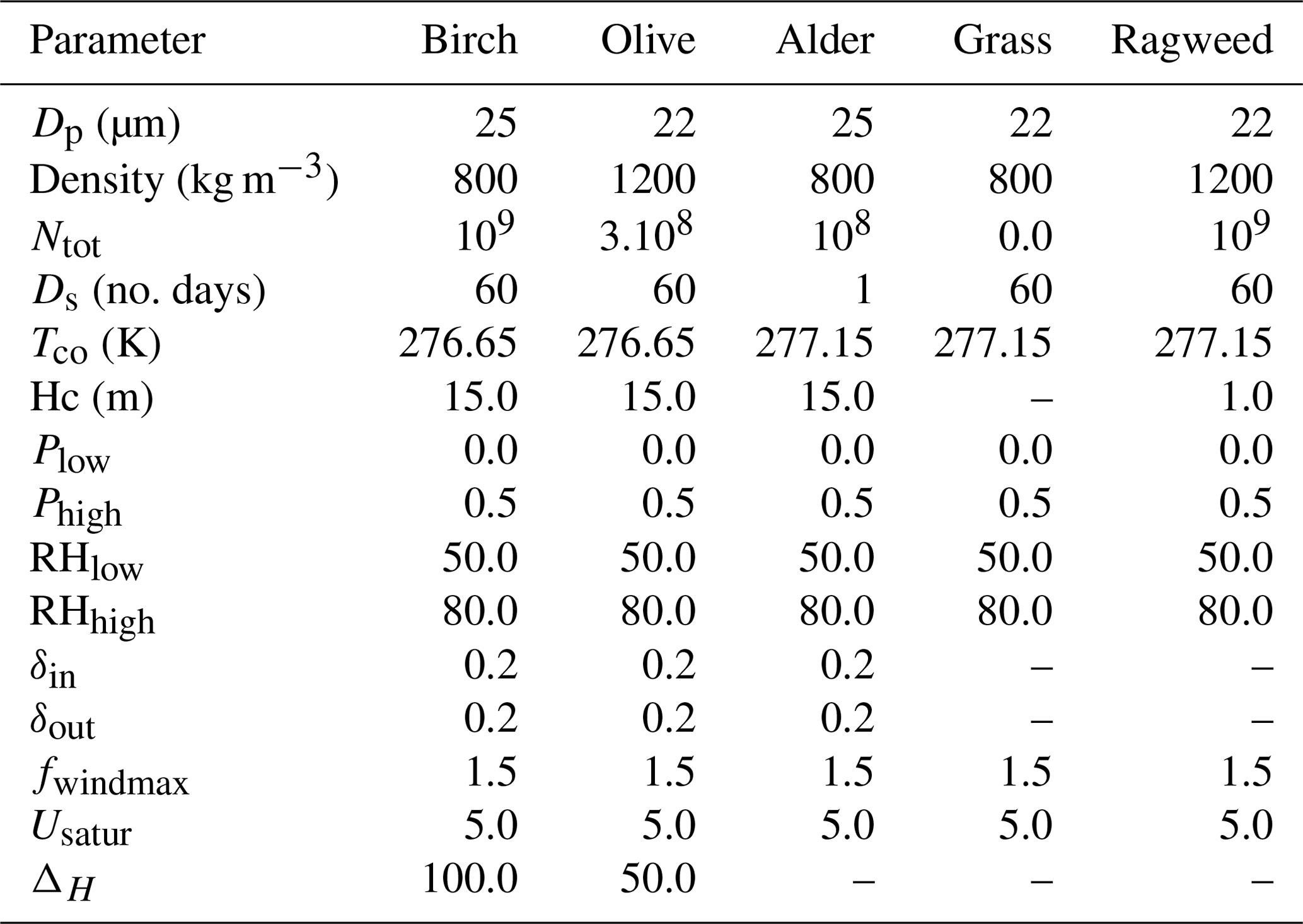
Precipitation and humidity impacts on the model are governed by the following equation, where xlow may be Plow or RHlow and xhigh may be Phigh or RHhigh. Depending on the pollen species, the values are fixed in Table 5.
Table 5Fixed parameters for the pollen emissions. Ntot is the total number of grains per square metre and year, Ds is the flowering start in Julian days, Tco is the temperature cutoff value (in K) and Hc is the emissions height.
The impacts of wind speed, U, and convective turbulence, w*, are described by
where Usatur corresponds to the maximum value where the wind still strengthens emissions and fwind-max describes the magnitude of wind impact. For birch, Usatur = 5 m s−1 and fwind-max = 1.5 (Table 5). All the trees of the same grid cell do not start flowering at the same time, with the transition between phenological stages being accomplished in a gradual manner. The gradual start of the flowering of the trees in a grid cell is described by the relative heat sum, , with the corresponding term Fin(x) given by
where δin is the relative uncertainty in Hstart. The parameter controlling the gradual flowering season termination is the number of grains remaining in catkins with respect to the initial total number of grains, Ntot, with . In the current model version, Ntot is fixed; for example, Ntot=109 for birch. The corresponding term Fout(x) is given by
where δout is the relative uncertainty in Ntot.
To simulate the pollen emission flux, the tree spatial distribution maps for each species are required. For birch, it was compiled by Sofiev et al. (2006) from a combination of national forest inventories of western Europe and satellite images of broadleaf forests when the former information was not available. The forest inventories reveal irregularities, which are probably related to the specifics of national methodologies for forest surveys. The use of satellite images allows one to smooth out the data between the countries. Some interpolations were made based on assumptions like if between 62° N and 65° N, the fraction of birch is expected to be equal to that found in Finland (80 %). In France, birch is mainly present in the Massif Central (middle mountain region), the west (Aquitaine Basin), and the north-east (the Vosges). As noted by Sofiev et al. (2013), there are noticeable regional variations in the temperature sum threshold that are necessary to trigger the flowering season. Hence, the temperature sum thresholds were fitted into phenological and aerobiological observations independently inside 33 sub-regions of Europe. This yielded a temperature sum threshold map for the flowering season start.
6.2.3 The heat sum concept
The heat sum (HS) concept follows the concept of Chapman et al. (2014), which is based on biological days. Some input information is necessary to update HS at each model time step: the current 2 m temperature, the current day, its length in hours and the time step. The HS is updated only if the current day is after the first day, which in our case is always equal to 79 (i.e. 20 March). Two ramp functions are estimated, one depending on the 2 m temperature and the second one on the day length. All data used are the same as in SILAM, as described in Prank et al. (2013), using parameters defined in Deen et al. (1998). The HS is then equal to
with
where the lh variable is equal to 1 except if the day length (dl) is greater than the photo period parameter, which is 14.5 here, and for the following values:
where the threshold temperature values are fixed. Note that this HS may be set to zero again depending on specific meteorological conditions as follows:
-
T2 m is lower than Tthr (here, Tthr=273.15 K).
-
Daily mean T2 m is lower than dayTthr (here, dayTthr=280.65 K). Note that in this model version, the daily mean 2 m temperature is the running average for the last 24 h.
-
HS is lower than StartHSThr. This value is fixed to StartHSThr = 25.0 here following Deen et al. (1998).
With this scheme, there are no emissions during the night. The calculation of sunrise and sunset is necessary. At the end, note that emissions are injected in the first model level only in CHIMERE, whereas they are injected in the whole boundary layer in SILAM.
6.2.4 The ragweed emission
The ragweed pollen emission is a specific case. It is possible to use the P2013 scheme, but two others are also implemented. The first one is the scheme developed by Efstathiou et al. (2011) that corresponds to a modified version of Helbig et al. (2004). The second one is the scheme of Menut et al. (2021b), which corresponds to a modified version of Efstathiou et al. (2011).
The approach of Efstathiou et al. (2011), hereafter called E2011, is a mix between the schemes of Helbig et al. (2004) and Sofiev et al. (2006), adapting these formulations to ragweed. In the following, the specific notations of the publications are used to have a reference. The terminology is different from P2013 and Helbig et al. (2004), but the principle is the same. The pollen emission flux, E (grains m−2 s−1), is calculated as
The flux depending on the surface grid cell and time is . The terms of the equation are ce, a plant-specific factor, and c*, the grain production factor. The release factor, Re, is represented by . Ke is a time-varying factor that depends on weather and u* is the friction velocity. The plant-specific factor, ce, is calculated as
where cb is approximated to 10−4. S is the pollen season duration in days, with S=60. d is the Julian day, which varies during the simulation. In practice, the starting and ending dates of the ragweed period are fixed to 210 and 270 Julian days here, respectively. The grain production factor, c*, is calculated as
where qp is the total production of grains per year and is 109 grains m−2. It corresponds to the maximum number of emitted grains. Day after day, qp is reduced by the number of the already emitted grains the day before. LAI is the leaf area index. LAI is a map in E2011, but in this CHIMERE version, we are using the value of LAI = 3. hc=1 m is the canopy height. The Ke variable is estimated by
with the three meteorological limiting factors: Kh for humidity, Kw for 10 m wind speed and Kr for precipitation. For relative humidity, the limiting factor is expressed as Eq. (45), with qlow=50 % and qhigh=80 %. For precipitation, we use the fit in E2011:
with p being the precipitation rate (in mm h−1). For the wind speed, Kw is based on the P2013 wind speed correction, previously described by Eq. (46).
The Menut et al. (2021b) scheme, hereafter called M2021, has the same formulation as the E2011 scheme, except that the release term is reformulated. The emission flux is expressed as
where ce and c* are the same functions as in the E2011 scheme. RTS is the modified instantaneous release factor. Based on the correlation results in M2021, it appears that the main driving factors are those related to thermodynamical processes – namely the 2 m temperature, T2 m; vertical velocity scale, w*; and short-wave radiation, SWd. The pollen emissions may be moderated by the precipitation rate, Pr, and 2 m specific humidity, q2 m.
The differences between birch and ragweed emissions could be explained by the plant typology itself: birch is a tree, with the pollen source up to 10 m above the ground. At this level, the wind may be considered a dominant process for the emission of grains. Ragweed rarely exceeds 1 to 2 m above the ground, where the wind speed is moderate. In this case, the dominant factor could be the temperature, considering the grains are emitted at the highest temperature when they are sufficiently dry (Holmes and Bassett, 1963). The precipitation rate is a limiting factor but not the most important one: even if it rains during the night, the grains can dry out and can be pulled off the plant in the morning. RTS is thus estimated as
where the values of T2 m, w* and SWd correspond to the mean daily values. These values are normalized in order to keep the release term non-dimensional. The normalization factors are °C, m s−1 and W m−2.
In order to moderate these fluxes when meteorological conditions are not favourable, resistance terms are added. These resistances are mainly due to the 2 m specific humidity, q2 m, and the precipitation rate, Pr. Each resistance is expressed as a sigmoid function ranging between 0 and 1, depending on the minimum and maximum value of the x parameter. The resistance has to reflect the fact that these parameters inhibit ragweed pollen emissions.
with bf being a constant, chosen here to be bf=10, that determines the curve of the sigmoid function. imin and imax represent the range of the sigmoid and are chosen here to be imin=0 and imax=1 in order to use a normalized function for each resistance. The critical issue here is to choose the minimum and maximum value for each x meteorological parameter. These boundaries have to reflect the best possible range of variations in meteorological variables for all locations over Europe and for the whole year. The maximum values must be moderate enough in order to provide a realistic resistance: a too low of a maximum value would give a resistance of 1 too often, while a too high of a maximum value would give resistances that are too low. Based on all meteorological values used in this study, the boundaries for the 2 m specific humidity are q2 m(min)=0 and g g−1 and for the precipitation rate are Pr(min)=0 and Pr(max)=1.5 mm h−1.
6.3 Changes in mineral dust emission
Two main novelties were developed in this model version. First, the way to calculate the fluxes is now following a sub-grid-scale variability, blending the percentages of soil in each percentage of land use and the Weibull distribution for the surface wind speed. It enables the calculation of a flux whatever the horizontal resolution is and as if it was at high resolution. Second, a link was added between vegetation fire emissions and mineral dust emissions (user's choice). We consider that vegetation fires are changing the soil and land use properties then create more erodible surfaces. In addition and during the fire, a vertical injection profile is applied to dust emission, considering that the fires induce a local convection.
6.3.1 Sub-grid-scale variability in the soil and land use
The principle of the calculation of emission flux was reshaped to be more efficient. The principle of sub-grid-scale variability is used. The main goal is to remove, as far as possible, the problem associated with the horizontal resolution when using emission schemes based on the threshold calculation principle. Thus, emission fluxes are calculated at the highest possible resolution and then summed up in the grid cell. For that, the input databases are pre-processed to have sub-grid tables, as presented in Fig. 4. In this figure, the big square represents a CHIMERE grid cell (here, for example, with a size of 8 km, with each sub-square at a resolution of 1 km). For each grid cell, we count the number of different land use classes and the number of different soil types. It defines a table as being a matrix and containing the relative part of each land use class in each soil type. For each value, we also attach the value of the saltation roughness length, z0, and the MODIS erodibility, also with a 1 km resolution. After calculation of all values, the table is sorted as a function of the land use for each soil. Later, in CHIMERE, the sorted table enables us to optimize the calculation speed by exiting the loop when the land use relative part becomes zero.
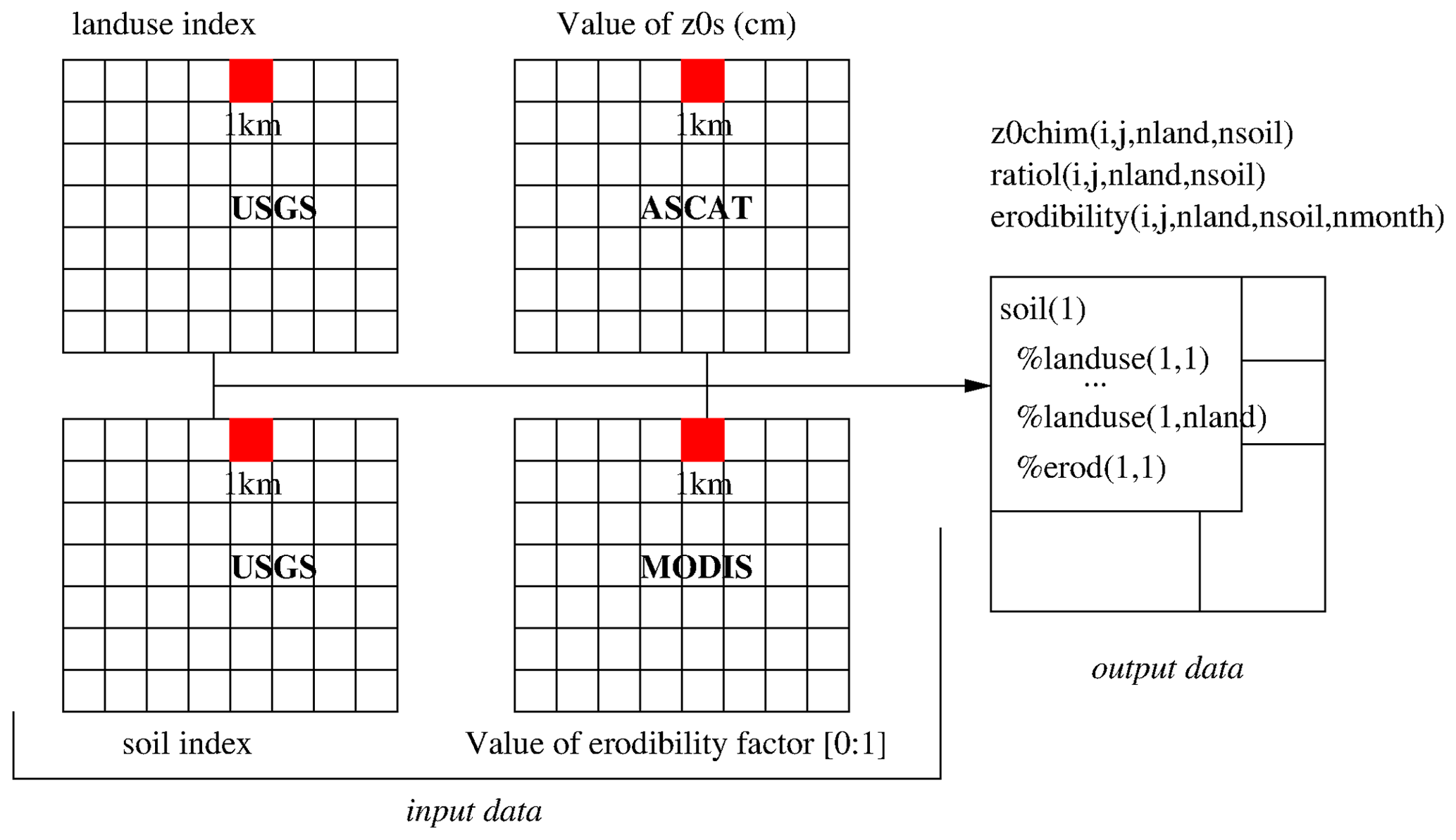
Figure 4The three datasets (kilometric resolution) are read together to build sub-grid-scale variability tables. For each cell, the relative percentage of land use for each soil type is calculated (ratiol) as well as the corresponding aeolian roughness length (z0chim).
The interesting part is that we can calculate mineral dust flux using threshold parameters such as aeolian roughness length as if we had a 1 km × 1 km horizontal resolution. With the sorted table, the calculation is fast. The weakness is that with this sub-grid-scale approach, we lost the spatial position of the high resolution: we know there is n % of land use, but we do not know where it is in the grid cell. Note it is not very important because we use the mean wind speed for the emissions calculation. For each sub-grid part, the emission flux calculation is done by iterating the Weibull distribution.
6.3.2 Impact of the fires on dust
Vegetation fire emission is parameterized using the emifiresCAMS program, which reads the CAMS daily data. For each day, the data provide information on the chemical species flux and on fire radiative power. Based on the hypothesis (Menut et al., 2022), the burnt area is deduced from this fire radiative power (FRP) value. The burnt area surface is cumulated from a starting date and then considered surface, having lost its vegetation. In this model version, the surface recovery is not taken into account, but it is considered that this recovery can take years, whereas we only simulate a few months during and just after the fires. The information needed is only valid using the CAMS vegetation fire emissions because the specific information of the burnt area surface was specifically developed in the CHIMERE emifiresCAMS program.
The fires have several impacts. First, short-term impacts are modelled and active only during the fire: (i) the local pyroconvection creates a surface pressure gradient and then increases the surface wind speed and (ii) the pyroconvection induces a local thermal, quickly mixing the surface emission in the whole atmospheric column. It has the effect of increasing the surface emissions and then transporting these emissions vertically, when the usual emission model only distributes fluxes into the first vertical model level. Second, long-term effects are also parameterized: by burning the surface, vegetation fires create additional barren surfaces, with more erodible properties for the mineral dust emissions.
7.1 The settling velocity
The calculation of the settling velocity for aerosols has been updated using the AerSett v1 formulation (Mailler et al., 2023a). As described in Mailler et al. (2023b), the terminal fall speed of aerosols is calculated as
In Eq. (58), the slip correction factor, Cc, is obtained following the classical Davies (1945) formulation, where is the Knudsen number, D the particle diameter and λ the mean free path of molecules in the air:
As discussed in Mailler et al. (2023b), the value of v∞ obtained from Eq. (60) always stays within 2 % of the “theoretical” v∞ value obtained from the Clift and Gauvin (1971) parameterization but is 4 times as fast as a brute-force iterative calculation of v∞. For small particles (), Eq. (60) is replaced by just , changing the result by less than 1 %. This typically applies to all particles with D<10 µm, while for large particles, Eq. (60) takes into account the Clift and Gauvin (1971) large-particle drag correction factor.
7.2 Impact of fires on dry deposition
A new process was added in the model. The dry deposition fluxes depend on the leaf area index for the calculation of the surface resistance, rc (Simpson et al., 2012). More precisely, the bulk canopy resistance is expressed as
where LAI is the leaf area index (in m2 m−2), gsto the stomatal conductance and Gns the bulk non-stomatal conductance.
In the case of using fire emissions (user's choice), we consider a new impact on this model version: the fires destroy the vegetation and modify the soil properties (a soil that is drier and more erodible). It has an impact on not only the mineral dust emissions (as described in Sect. 6.3.2), but also the vegetation and then the LAI. The effect of the fires is cumulated in time for that moment from the beginning of each year. For the LAI, its decrease due to the fires is expressed as
where Stotal is the total surface of the grid cell when a fire is active or was previously diagnosed. Sburnt is the time-cumulated burnt surface.
7.3 Update to the ISORROPIA module
The ISORROPIA module has been used for a long time in the model in order to simulate the partitioning of inorganic aerosols (Nenes et al., 1998). This module was originally written in Fortran 77 and is used in both its forward and reverse modes in CHIMERE. In order to solve possible instability issues as well as increase the readability of the module, we opted to use a Fortran 90 version of ISORROPIA.
This was partially done by adapting the ISORROPIA module used in the GEOS-Chem (The International GEOS-Chem User Community, 2021) model for CHIMERE. Since GEOS-Chem only uses the forward mode of ISORROPIA, we opted to add the reverse mode into the module. The entirely translated version was then tested both outside (in a zero-dimensional configuration) and inside CHIMERE. It was concluded that the two modules provide the same results, while the Fortran 90 version of the module is more stable than the Fortran 77 version. This stable version is now part of the CHIMERE model.
8.1 Simulation and validation setup
The model goes through continuous quality control validations. Six simulations are designed: first, with two model versions, (i) with the previous model version, v2020r3, and (ii) with this new version, v2023r1, and second, for each version, with three different configurations: (i) in offline mode and forced by ECMWF meteorological fields; (ii) in offline mode and forced by WRF 4.3; and (iii) in online mode, also forced by WRF 4.3. These three configurations are chosen since they show the results of the model with two major meteorological forcings as well as the effect of coupling with an online meteorological model on the simulated concentrations.
The simulations are performed over a domain that covers most of Europe and northern Africa. This domain is usually used for validation purposes since it takes into account a region containing all the possible emission sources in the model, i.e. anthropogenic, biogenic, biomass burning, sea salt and dust sources. The horizontal resolution of the model is 60 km × 60 km. The vertical resolution of the model has 15 levels, starting from the surface and going up to 300 hPa. The simulations are performed for the entire year of 2019 in order to take into account seasonal changes. For simulations using WRF, this model is forced by the CFSv2 meteorological inputs (Saha et al., 2011); for simulations using ECMWF, the meteorology from the IFS/ECMWF fields, with a 0.25×0.25° global resolution and 3-hourly time frequency, is used. Anthropogenic emissions come from the CAMS global emission inventory (v5.3; Soulie et al., 2024). Mineral dust, salt, DMS, anthropogenic, biogenic and NOx emissions from lightning have all been calculated. The CAMS global reanalysis 6-hourly fields are used as initial/boundary conditions. The CHIMERE model is run with 10 aerosol size bins starting from 10 nm and going up to 40 µm.
For the calculation of statistical scores, the EvalTools module is used. It is a Python package developed by INERIS and Météo-France and freely available on a website (version 1.0.6r; https://opensource.umr-cnrm.fr/projects/evaltools, last access: 9 July 2024). Being also used by INERIS in the framework of the daily operational forecast using CHIMERE over France (PREV'AIR) and Europe (CAMS Copernicus), the advantage of using this tool is to be completely homogeneous with the validation made for the operational forecast.
Measurements used for these comparisons are collected from multiple sources. The model is validated on a regular basis with a vast amount of data for a large list of species downloaded from several sources. Starting with the meteorological data, 2 m temperature, wind speed, precipitation and relative humidity are compared. These measurements come from E-OBS, the British Atmospheric Data Centre network (BADC; http://data.ceda.ac.uk/badc, last access: 6 December 2023) and EBAS (https://ebas-data.nilu.no/, last access: 6 December 2023). The E-OBS dataset (prepared by the ECA&D project) provides daily data on a regular 0.1×0.25 grid covering the European area. For all variables provided by E-OBS, data for the European Environment Agency (EEA) ozone (O3) stations are extracted from the gridded format and compared to the simulations.
For atmospheric pollutants, a long list of species is compared to the simulations on a regular basis, but only certain comparisons are presented in this paper. Ground-level measurements of O3, PM10 and PM2.5 are downloaded from the European Environment Agency (EEA; https://www.eea.europa. eu, last access: 6 December 2023), EBAS and OpenAQ (https://openaq.org/, last access: 6 December 2023). The observations for aerosol optical depth (AOD) downloaded from the Aerosol RObotic NETwork global remote sensing network (AERONET; https://aeronet.gsfc.nasa.gov/, last access: 6 December 2023) are also included.
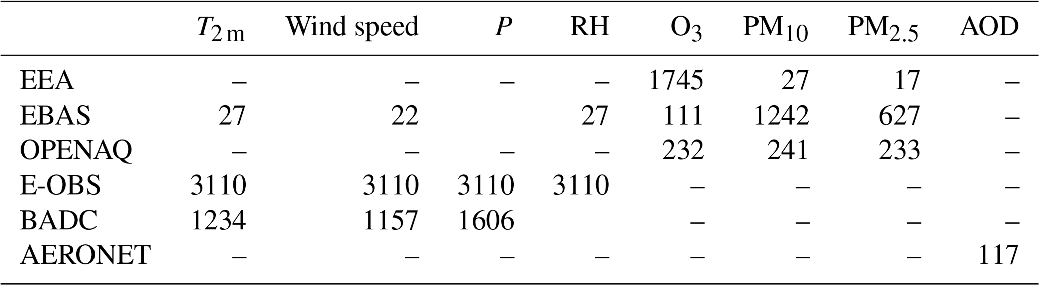
The comparisons have been performed for all types of stations. It should be noted that all the data mentioned here are at an hourly resolution, apart from the E-OBS data. Only stations with at least 90 % data availability threshold for the entire year of 2019 have been used. An exception has been given to the AOD data, where the data availability during the year has been fixed at 25 %. The number of stations used for each of these sources is given in Table 6.
We have also included validation for vertical profiles of pressure, temperature and O3 using the data acquired from the World Ozone and Ultraviolet Radiation Data Centre (WOUDC; https://woudc.org/home.php, last access: 6 December 2023) resulting from ozonesonde measurements. There are 700 balloon flights inside the simulation domain that have sufficient data for the year from nine locations. Only stations with over 25 flights during the year were used for the comparisons.
8.2 Statistical scores
Statistical scores are presented for O3, PM2.5 and PM10 surface concentrations and aerosol optical depth (AOD). The scores are calculated for six model configurations: the previous model version, v2020r3, and the new model version, v2023r1, with three different meteorological forcings – ECMWF in offline mode, called offecm, and WRF in offline and online modes, respectively, called offwrf and onwrf.
Results for ozone surface concentrations are presented in Fig. 5. In the top part of the figure, the hourly mean bias is presented for the six simulations, with the three v2020r3 configurations on the left and the three v2023r1 configurations on the right. For each, results are calculated for the three datasets (EBAS, EEA and OpenAQ). With the old version, the bias is large and negative when compared to EBAS but close to zero when compared to EEA and OpenAQ. With the new version, the bias becomes low for EBAS and positive and much larger for EEA and OpenAQ. It means that independently of the surface dataset and independently of the offline or online mode, the new version simulates more hourly ozone than the previous one. This difference may reach +12.19 and +10.4 µg m−3 when v2023r1_onwrf simulations are compared to EEA and OpenAQ, respectively. It means that compared to the previous version, there is a positive shift of /+10 µg m−3 for the surface ozone concentrations.
For the correlation (bottom of Fig. 5), the values show an increase between the old model version and the new one. For example, for onwrf, correlation increases from 0.55 to 0.65 with EBAS, from 0.61 to 0.70 with EEA and from 0.63 to 0.71 with OpenAQ. This increase is noted for the three model configurations, with or without direct/indirect effects. On average, the new model version provides correlation with an increase of +0.07 for ozone.
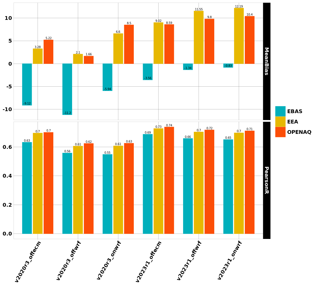
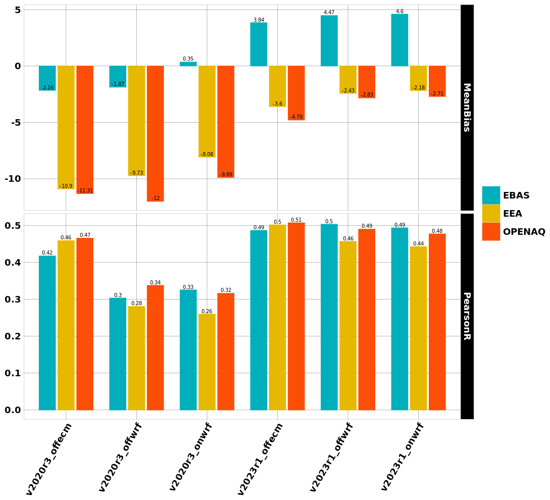
Figure 6 presents the same kind of validation but for PM10 surface concentrations. The mean bias is reduced for all simulations and changes from largely negative to slightly positive. For example and for the online coupling, the bias of −8.08 and −9.89 µg m−3 for the comparison to EEA and OpenAQ changes to −2.18 and −2.71 µg m−3 with the v2023r1 model version. On the other hand and by comparison to EBAS data, the bias changes from 0.35 to 4.6 µg m−3. On average, the surface concentrations of PM10 increase by ≈5 µg m−3 for all model configurations of v2023r1 compared to v2020r3. As for ozone, the correlation systematically increases with the new model version. If we consider the validation by comparison to EEA data, we can see an increase from 0.46 to 0.50 when the meteorological forcing is offecm. The increase is much larger when the meteorological forcing is the WRF model, with, for example, an increase from 0.26 to 0.44 for onwrf between the old and the new model version. On average, the gain in correlation is roughly +0.05 when the forcing is offecm and +0.2 when the forcing is offwrf or onwrf.
The same kind of validation is performed for aerosol optical depth, and results are presented in Fig. 7. The only dataset here is AERONET, providing a large geographical cover of the AOD. Regarding the bias, it is slightly reduced between the old and the new model version, but the differences between the old and the new version are very low. The bias was also smaller when using offwrf and onwrf in place of offecm. This result remains the same with the new model version. The correlation changes with the new version. With offecm, one can note an increase from 0.55 to 0.59. With offwrf and onwrf, the increase is much larger, with values from 0.33 and 0.32 for v2020r3 to 0.64 and 0.64 for v2023r1. Depending on the meteorological forcing, the net gain in AOD correlation ranges from +0.05 to +0.3. The use of the new version is always a gain.
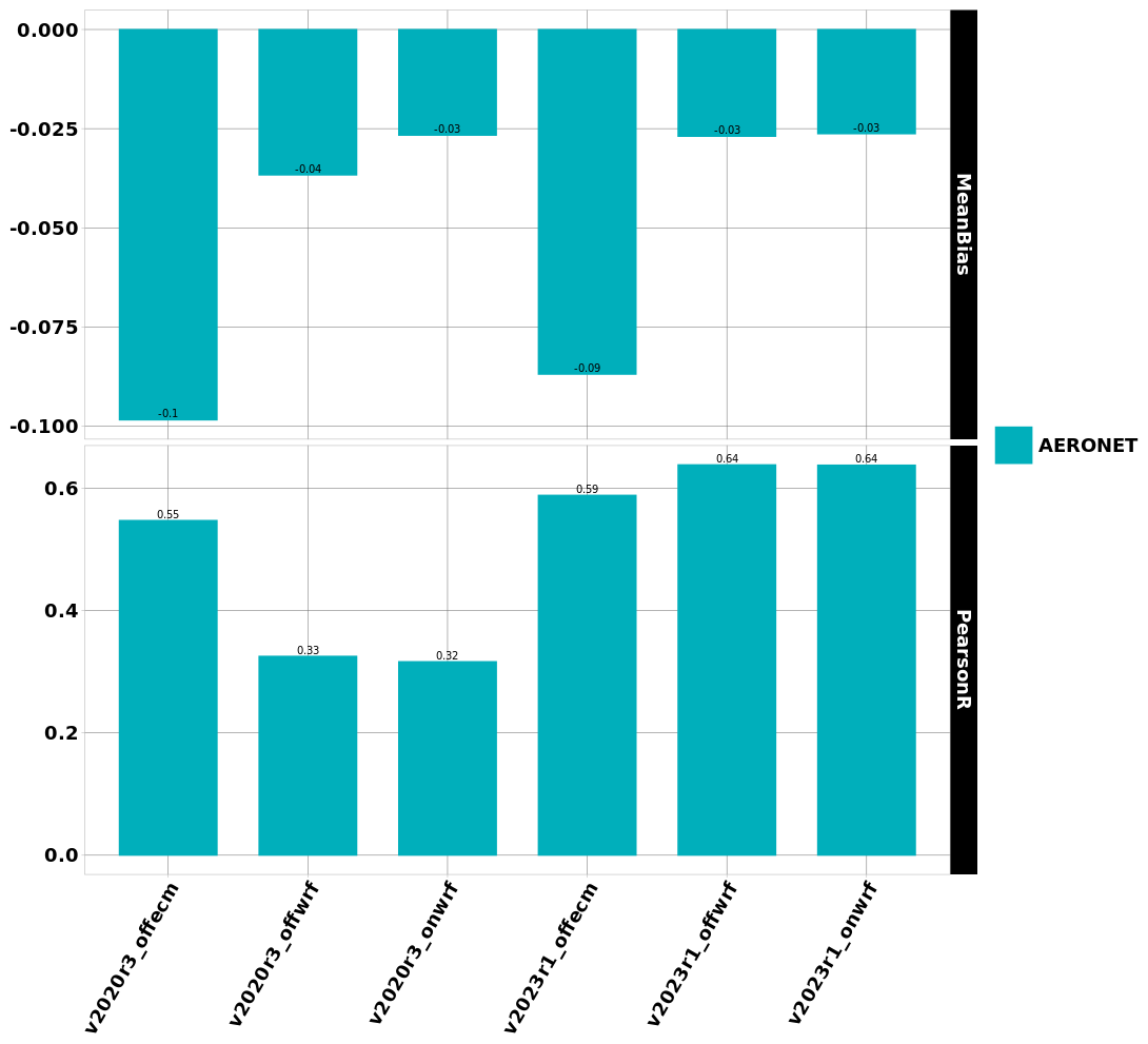
Another way to validate the simulations with the new model version is to compare model outputs to vertical soundings. Results are synthesized in Fig. 8 for ozone. All soundings recorded during the simulation period (1 year) and over the whole domain are aggregated to calculate bias and correlation. Values are presented at the vertical model levels. The values for observations are thus presented as the mean average (the black bar and dot) and the standard deviation as a black dot in a coloured bar. At each level, the correlation is presented as coloured text: the colour corresponds to the model configuration with the best correlation. It enables us to easily visualize where model configurations outperform the average. For this simulation, the best scores are obtained with v2023r1 forced offline, with WRF close to the surface and then with the offline ECMWF version for the rest of the tropospheric column (except two model levels, where the best score is obtained with v2020r3). Globally, the best scores are with v2023r1, in the configuration forced by ECMWF. It is also noticeable that the standard deviation values at each model level are very close between observations and the model. It changes only close to the top, where the model variability becomes larger than the observations. At these levels, the boundary conditions play a role in this variability.
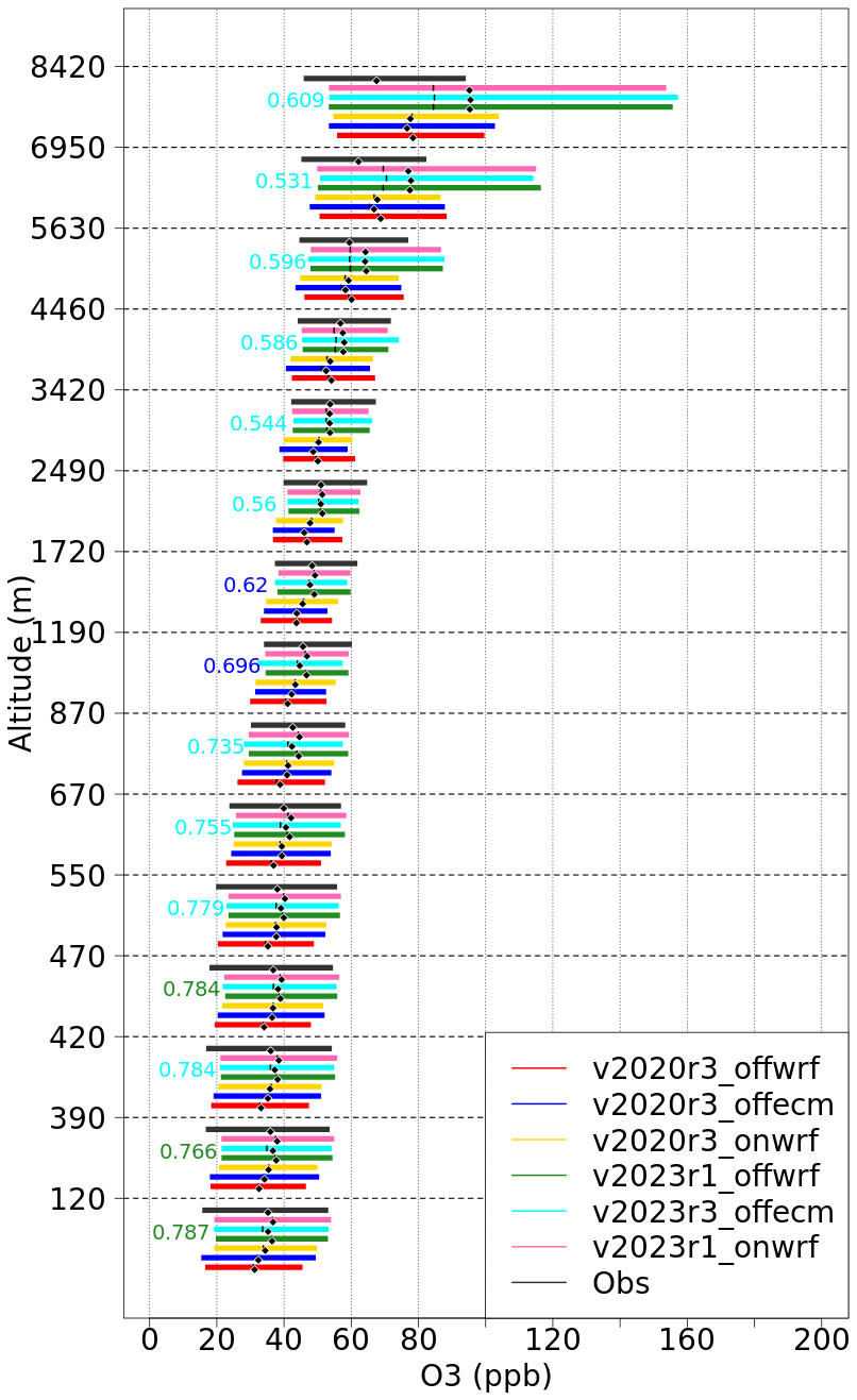
Figure 8Comparison between observations and model results as a mean averaged vertical profile of ozone (in ppb). The data are averaged over the whole modelled period and for all available vertical soundings recorded over Europe.
The new CHIMERE version called v2023r1 is presented in this article. It contains both new processes and new numerical tools. More precisely for the researchers, the pollen emissions are now distributed and can be used for any local studies in Europe, the turbulence and the transport were updated with more recent parameterizations, and the impact of the fires on the surface was added. For the users performing long simulations or forecast, the integration of the XIOS model enables us to have a faster model, with a computational cost that is 40 % lower than the previous version. It is also possible to easily manage the output, including the possibility of writing sub-hourly fields, such as the maximum concentration during an hour.
The perspectives for the model are to continue to modularize the code and to optimize the calculation. The future of such a model being to go toward high-performance computing (HPC) architecture, it is important to follow the fast evolution in numeric methodology, including optimization. The use of XIOS for reading input data will also be implemented to allow some on-the-fly interpolation in the case of complex grids.
Table A1USGS land use types and minimum and maximum values of momentum roughness length z0.
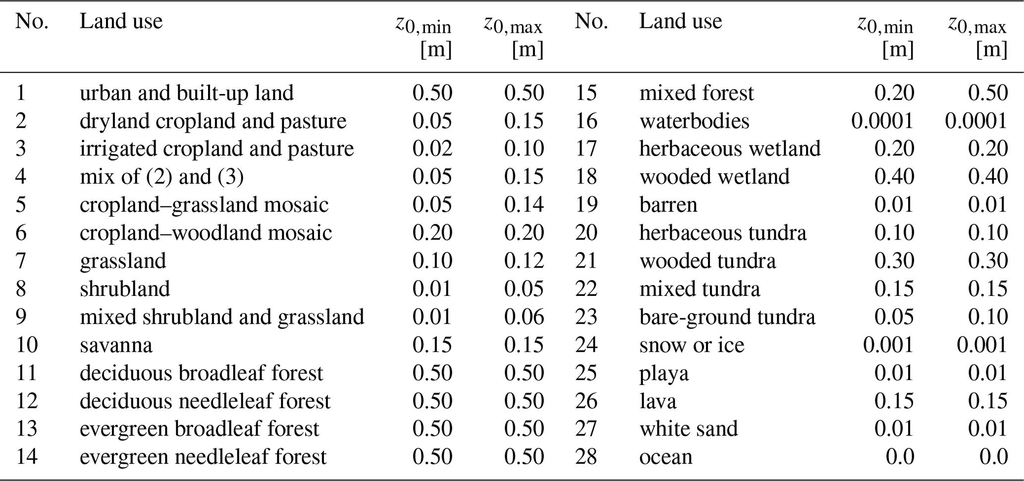
Table A2USGS land use types and tabulated albedos for bare and snow surfaces.
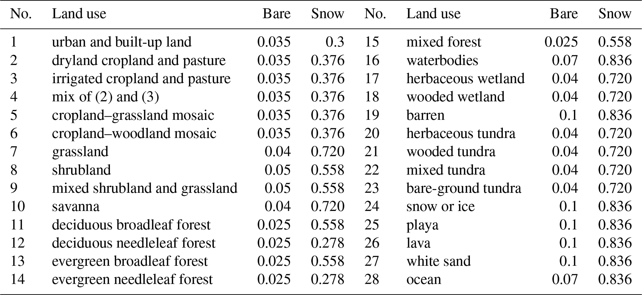
The CHIMERE v2023r1 model is available on Zenodo at https://doi.org/10.5281/zenodo.10907951 (Menut et al., 2024).
All data used in this study as well as the data required to run the simulations are available on the CHIMERE website at https://www.lmd.polytechnique.fr/chimere (LMD Polytechnique, 2023).
All authors contributed to the model development. LM coordinated the paper and all authors wrote a part and reviewed it.
The contact author has declared that none of the authors has any competing interests.
Publisher's note: Copernicus Publications remains neutral with regard to jurisdictional claims made in the text, published maps, institutional affiliations, or any other geographical representation in this paper. While Copernicus Publications makes every effort to include appropriate place names, the final responsibility lies with the authors.
The authors acknowledge the OASIS modelling team for their support with the OASIS coupler, the WRF developer team for the free use of their model and Bertrand Bessagnet for continuous discussions about aerosol modelling. They also thank the investigators and staff who maintain and provide the AERONET data (https://aeronet.gsfc.nasa.gov/, last access: 9 July 2024). The European Environmental Agency (EEA) is acknowledged for their air quality station data that are provided and freely downloadable (https://www.eea.europa.eu/data-and-maps/data/aqereporting-8, last access: 9 July 2024). This work was granted access to the HPC resources of TGCC and IDRIS under the allocation no. 2023-A0130110274 made by GENCI.
Centre National de la Recherche Scientifique (CNRS) with the Institut National des Sciences de l'Univers (INSU) provided funding that supported the development of CHIMERE, labelled as a national tool of French research.
This paper was edited by Samuel Remy and reviewed by three anonymous referees.
Arnfield, A. J.: Two decades of urban climate research: a review of turbulence, exchanges of energy and water, and the urban heat island, Int. J. Climatol., 23, 1–26, https://doi.org/10.1002/joc.859, 2003. a
Beegum, S., Gherboudj, I., Chaouch, N., Couvidat, F., Menut, L., and Ghedira, H.: Simulating Aerosols over Arabian Peninsula with CHIMERE: Sensitivity to soil, surface parameters and anthropogenic emission inventories, Atmos. Environ., 128, 185–197, https://doi.org/10.1016/j.atmosenv.2016.01.010, 2016. a
Beljaars, A. C. M. and Holtslag, A. A. M.: Flux Parameterization over Land Surfaces for Atmospheric Models, J. Appl. Meteorol., 30, 327–341, https://doi.org/10.1175/1520-0450(1991)030<0327:FPOLSF>2.0.CO;2, 1991. a, b
Beljaars, A. C. M. and Viterbo, P.: The sensitivity of winter evaporation to the formulation of aerodynamic resistance in the ECMWF model, Bound.-Lay. Meteorol., 71, 135–149, https://doi.org/10.1007/BF00709223, 1994. a
Betts, A., Hong, S., and Pan, H.: Comparison of NCEP-NCAR Realanalysis with 1987 FIFE data, Mon. Weather Rev., 124, 1480–1498, https://doi.org/10.1175/1520-0493(1996)124<1480:connrw>2.0.co;2, 1995. a, b
Boucher, O., Servonnat, J., Albright, A. L., et al.: Presentation and evaluation of the IPSL-CM6A-LR climate model, J. Adv. Model. Earth Sy., 12, e2019MS002010, https://doi.org/10.1029/2019MS002010, 2020. a
Bruin, H. A. R. D. and Holtslag, A. A. M.: A Simple Parameterization of the Surface Fluxes of Sensible and Latent Heat During Daytime Compared with the Penman-Monteith Concept, J. Appl. Meteorol. Climatol., 21, 1610–1621, https://doi.org/10.1175/1520-0450(1982)021<1610:ASPOTS>2.0.CO;2, 1982. a, b
Calbo, J., Pan, W., Webster, M., Prinn, R. G., and McRae, G. J.: Parameterization of urban subgrid scale processes in global atmospheric chemistry models, J. Geophys. Res.-Atmos., 103, 3437–3451, https://doi.org/10.1029/97JD02654, 1998. a
Carter, W.: Development of the SAPRC-07 chemical mechanism, Atmos. Environ., 44, 5324–5335, https://doi.org/10.1016/j.atmosenv.2010.01.026, 2010. a
Chapman, D. S., Haynes, T., Beal, S., Essl, F., and Bullock, J. M.: Phenology predicts the native and invasive range limits of common ragweed, Global Change Biol., 20, 192–202, https://doi.org/10.1111/gcb.12380, 2014. a
Charnock, H.: Wind stress over a water surface, Q. J. Roy. Meteor. Soc., 81, 639–640, 1955. a, b
Cheinet, S. and Teixeira, J.: A simple formulation for the eddy-diffusivity parameterization of cloud-topped boundary layers, Geophys. Res. Lett., 30, 1930, https://doi.org/10.1029/2003GL017377, 2003. a
Clift, R. and Gauvin, W. H.: Motion of entrained particles in gas streams, Can. J. Chem. Eng., 49, 439–448, https://doi.org/10.1002/cjce.5450490403, 1971. a, b
Colella, P. and Woodward, P. R.: The piecewise parabolic method (PPM) for gas-dynamical simulations, J. Comput. Phys., 11, 38–39, 1984. a
Courant, R., Issacson, E., and Reees, M.: On the Solution of Nonlinear Hyperbolic Differential Equations by Finite Differences, Comm. Pure Appl. Math., 5, 243–255, 1952. a
Craig, A., Valcke, S., and Coquart, L.: Development and performance of a new version of the OASIS coupler, OASIS3-MCT_3.0, Geosci. Model Dev., 10, 3297–3308, https://doi.org/10.5194/gmd-10-3297-2017, 2017. a
Crippa, M., Solazzo, E., Huang, G., Guizzardi, D., Koffi, E., Muntean, M., Schieberle, C., Friedrich, R., and Janssens-Maenhout, G.: High resolution temporal profiles in the Emissions Database for Global Atmospheric Research, Sci Data, 7, 121, https://doi.org/10.1038/s41597-020-0462-2, 2020. a
Davies, C. N.: Definitive equations for the fluid resistance of spheres, Proc. Phys. Soc., 57, 259–270, https://doi.org/10.1088/0959-5309/57/4/301, 1945. a
Deen, W., Hunt, L. A., and Swanton, C. J.: Photothermal time describes common ragweed (Ambrosia artemisiifolia L.) phenological development and growth, Weed Sci., 46, 561–568, https://doi.org/10.1017/S0043174500091104, 1998. a, b
Deroubaix, A., Menut, L., Flamant, C., Brito, J., Denjean, C., Dreiling, V., Fink, A., Jambert, C., Kalthoff, N., Knippertz, P., Ladkin, R., Mailler, S., Maranan, M., Pacifico, F., Piguet, B., Siour, G., and Turquety, S.: Diurnal cycle of coastal anthropogenic pollutant transport over southern West Africa during the DACCIWA campaign, Atmos. Chem. Phys., 19, 473–497, https://doi.org/10.5194/acp-19-473-2019, 2019. a
Després, B. and Lagoutière, F.: Un schéma non linéaire anti-dissipatif pour l'équation d'advection linéaire, Comptes Rendus de l'Académie des Sciences – Series I – Mathematics, 328, 939–943, https://doi.org/10.1016/S0764-4442(99)80301-2, 1999. a, b
Efstathiou, C., Isukapalli, S., and Georgopoulos, P.: A mechanistic modeling system for estimating large-scale emissions and transport of pollen and co-allergens, Atmos. Environ., 45, 2260–2276, https://doi.org/10.1016/j.atmosenv.2010.12.008, 2011. a, b, c, d
Emberson, L.-D., Ashmore, M.-R., Simpson, D., Tuovinen, J.-P., and Cambridge, H.-M.: Modelling and mapping ozone deposition in Europe, Water Air Soil Pollut., 130, 577–582, 2001. a
Feng, X., Sun, J., Yang, D., Yin, B., Gao, G., and Wan, W.: Effect of Drag Coefficient Parameterizations on Air–Sea Coupled Simulations: A Case Study for Typhoons Haima and Nida in 2016, J. Atmos. Ocean. Tech., 38, 977–993, https://doi.org/10.1175/JTECH-D-20-0133.1, 2021. a
Fuster, B., Sanchez-Zapero, J., Camacho, F., Garcia-Santos, V., Verger, A., Lacaze, R., Weiss, M., Baret, F., and Smets, B.: Quality Assessment of PROBA-V LAI, fAPAR and fCOVER Collection 300 m Products of Copernicus Global Land Service, Remote Sens., 12, 1017, https://doi.org/10.3390/rs12061017, 2020. a
Godunov, S. K. and Bohachevsky, I.: Finite difference method for numerical computation of discontinuous solutions of the equations of fluid dynamics, Matematičeskij sbornik, 47, 271–306, 1959. a
Grachev, A., Fairall, C., and Bradley, E.: Convective Profile Constants Revisited, Bound.-Lay. Meteorol., 94, 495–515, https://doi.org/10.1023/A:1002452529672, 2000. a
Guevara, M., Jorba, O., Tena, C., Denier van der Gon, H., Kuenen, J., Elguindi, N., Darras, S., Granier, C., and Pérez García-Pando, C.: Copernicus Atmosphere Monitoring Service TEMPOral profiles (CAMS-TEMPO): global and European emission temporal profile maps for atmospheric chemistry modelling, Earth Syst. Sci. Data, 13, 367–404, https://doi.org/10.5194/essd-13-367-2021, 2021. a
Helbig, N., Vogel, B., Vogel, H., and Fiedler, F.: Numerical modelling of pollen dispersion on the regional scale, Aerobiologia, 3, 3–19, 2004. a, b, c
Hersbach, H.: Sea Surface Roughness and Drag Coefficient as Functions of Neutral Wind Speed, J. Phys. Oceanogr., 41, 247–251, https://doi.org/10.1175/2010JPO4567.1, 2011. a
Holmes, R. and Bassett, I.: Effect of meteorological events on ragweed pollen count, Int. J. Biometeorol., 7, 27–34, 1963. a
Jiménez, P. A., Dudhia, J., González-Rouco, J. F., Navarro, J., Montávez, J. P., and Garcia-Bustamante, E.: A Revised Scheme for the WRF Surface Layer Formulation, Mon. Weather Rev., 140, 898–918, https://doi.org/10.1175/MWR-D-11-00056.1, 2012. a, b, c
Journet, E., Balkanski, Y., and Harrison, S. P.: A new data set of soil mineralogy for dust-cycle modeling, Atmos. Chem. Phys., 14, 3801–3816, https://doi.org/10.5194/acp-14-3801-2014, 2014. a
Lachatre, M., Mailler, S., Menut, L., Turquety, S., Sellitto, P., Guermazi, H., Salerno, G., Caltabiano, T., and Carboni, E.: New strategies for vertical transport in chemistry transport models: application to the case of the Mount Etna eruption on 18 March 2012 with CHIMERE v2017r4, Geosci. Model Dev., 13, 5707–5723, https://doi.org/10.5194/gmd-13-5707-2020, 2020. a, b
Lachatre, M., Mailler, S., Menut, L., Cholakian, A., Sellitto, P., Siour, G., Guermazi, H., Salerno, G., and Giammanco, S.: Modelling SO2 conversion into sulfates in the mid-troposphere with a 3D chemistry transport model: the case of Mount Etna's eruption on 12 April 2012, Atmos. Chem. Phys., 22, 13861–13879, https://doi.org/10.5194/acp-22-13861-2022, 2022. a, b, c, d
Lana, A., Bell, T. G., Simo, R., Vallina, S. M., Ballabrera-Poy, J., Kettle, A. J., Dachs, J., Bopp, L., Saltzman, E. S., Stefels, J., Johnson, J. E., and Liss, P. S.: An updated climatology of surface dimethlysulfide concentrations and emission fluxes in the global ocean, Global Biogeochem. Cycles, 25, GB1004, https://doi.org/10.1029/2010GB003850, 2011. a
Lapere, R., Huneeus, N., Mailler, S., Menut, L., and Couvidat, F.: Meteorological export and deposition fluxes of black carbon on glaciers of the central Chilean Andes, Atmos. Chem. Phys., 23, 1749–1768, https://doi.org/10.5194/acp-23-1749-2023, 2023. a
Linkosalo, T., Ranta, H., Oksanen, A., Siljamo, P., Luomajoki, A., Kukkonen, J., and Sofiev, M.: A double-threshold temperature sum model for predicting the flowering duration and relative intensity of Betula pendula and B. pubescens, Agric. Forest Meteorol., 150, 1579–1584, https://doi.org/10.1016/j.agrformet.2010.08.007, 2010. a
LMD Polytechnique: CHIMERE, LMD Polytechnique [data set], https://www.lmd.polytechnique.fr/chimere (last access: 9 July 2024), 2023. a
Louis, J.: A parametric model of vertical eddy fluxes in the atmosphere, Bound.-Lay. Meteorol., 17, 187–202, 1979. a, b
Mailler, S., Menut, L., Khvorostyanov, D., Valari, M., Couvidat, F., Siour, G., Turquety, S., Briant, R., Tuccella, P., Bessagnet, B., Colette, A., Létinois, L., Markakis, K., and Meleux, F.: CHIMERE-2017: from urban to hemispheric chemistry-transport modeling, Geosci. Model Dev., 10, 2397–2423, https://doi.org/10.5194/gmd-10-2397-2017, 2017. a, b
Mailler, S., Menut, L., Cholakian, A., and Pennel, R.: AerSett, Zenodo [code], https://doi.org/10.5281/zenodo.7535115, 2023a. a
Mailler, S., Menut, L., Cholakian, A., and Pennel, R.: AerSett v1.0: a simple and straightforward model for the settling speed of big spherical atmospheric aerosols, Geosci. Model Dev., 16, 1119–1127, https://doi.org/10.5194/gmd-16-1119-2023, 2023b. a, b
Mailler, S., Pennel, R., Menut, L., and Cholakian, A.: An improved version of the piecewise parabolic method advection scheme: description and performance assessment in a bidimensional test case with stiff chemistry in toyCTM v1.0.1, Geosci. Model Dev., 16, 7509–7526, https://doi.org/10.5194/gmd-16-7509-2023, 2023c. a, b
Menut, L., Bessagnet, B., Khvorostyanov, D., Beekmann, M., Blond, N., Colette, A., Coll, I., Curci, G., Foret, G., Hodzic, A., Mailler, S., Meleux, F., Monge, J.-L., Pison, I., Siour, G., Turquety, S., Valari, M., Vautard, R., and Vivanco, M. G.: CHIMERE 2013: a model for regional atmospheric composition modelling, Geosci. Model Dev., 6, 981–1028, https://doi.org/10.5194/gmd-6-981-2013, 2013. a, b
Menut, L., Bessagnet, B., Briant, R., Cholakian, A., Couvidat, F., Mailler, S., Pennel, R., Siour, G., Tuccella, P., Turquety, S., and Valari, M.: The CHIMERE v2020r1 online chemistry-transport model, Geosci. Model Dev., 14, 6781–6811, https://doi.org/10.5194/gmd-14-6781-2021, 2021a. a, b
Menut, L., Khvorostyanov, D., Couvidat, F., and Meleux, F.: Impact of Ragweed Pollen Daily Release Intensity on Long-Range Transport in Western Europe, Atmosphere, 12, 693, https://doi.org/10.3390/atmos12060693, 2021b. a, b, c, d
Menut, L., Siour, G., Bessagnet, B., Cholakian, A., Pennel, R., and Mailler, S.: Impact of Wildfires on Mineral Dust Emissions in Europe, J. Geophys. Res.-Atmos., 127, e2022JD037395, https://doi.org/10.1029/2022JD037395, 2022. a
Menut, L., Cholakian, A., Siour, G., Lapere, R., Pennel, R., Mailler, S., and Bessagnet, B.: Impact of Landes forest fires on air quality in France during the 2022 summer, Atmos. Chem. Phys., 23, 7281–7296, https://doi.org/10.5194/acp-23-7281-2023, 2023. a
Menut, L., Cholakian, A., Pennel, R., Siour, G., Mailler, S., Valari, M., Lugon, L., and Meurdesoif, Y.: chimere_v2023r1 (2023r1), Zenodo [code], https://doi.org/10.5281/zenodo.10907951, 2024. a
Nenes, A., Pilinis, C., and Pandis, S.: ISORROPIA: A new thermodynamic model for inorganic multicomponent atmospheric aerosols, Aquat. Geochem., 4, 123–152, 1998. a
Oke, T. R.: The energetic basis of the urban heat island, Q. J. Roy. Meteor. Soc., 108, 1–24, https://doi.org/10.1002/qj.49710845502, 1982. a
Paulson, C. A.: The Mathematical Representation of Wind Speed and Temperature Profiles in the Unstable Atmospheric Surface Layer, J. Appl. Meteorol. Climatol., 9, 857–861, https://doi.org/10.1175/1520-0450(1970)009<0857:TMROWS>2.0.CO;2, 1970. a
Pena, A. and Gryning, S.-E.: Charnock's Roughness Length Model and Non-dimensional Wind Profiles Over the Sea, Bound.-Lay. Meteorol., 128, 191–203, https://doi.org/10.1007/s10546-008-9285-y, 2008. a
Prank, M., Chapman, D., Bullock, J., Belmonte, J., Berger, U., Dahl, A., Jager, S., Kovtunenko, I., Magyar, D., Niemela, S., Rantio-Lehtimaki, A., Rodinkova, V., Sauliene, I., Severova, E., Sikoparija, B., and Sofiev, M.: An operational model for forecasting ragweed pollen release and dispersion in Europe, Agric. Forest Meteorol., 182, 43–53, 2013. a, b, c
Prigent, C., Jiménez, C., and Catherinot, J.: Comparison of satellite microwave backscattering (ASCAT) and visible/near-infrared reflectances (PARASOL) for the estimation of aeolian aerodynamic roughness length in arid and semi-arid regions, Atmos. Meas. Tech., 5, 2703–2712, https://doi.org/10.5194/amt-5-2703-2012, 2012. a
Saha, S., Moorthi, S., Wu, X., Wang, J., Nadiga, S., Tripp, P., Behringer, D., Hou, Y.-T., ya Chuang, H., Iredell, M., Ek, M., Meng, J., Yang, R., Mendez, M. P., van den Dool, H., Zhang, Q., Wang, W., Chen, M., and Becker, E.: NCEP Climate Forecast System Version 2 (CFSv2) 6-hourly Products, Computational and Information Systems Laboratory [data set], https://doi.org/10.5065/D61C1TXF, 2011. a
Sartelet, K., Couvidat, F., Wang, Z., Flageul, C., and Kim, Y.: SSH-Aerosol v1.1: A Modular Box Model to Simulate the Evolution of Primary and Secondary Aerosols, Atmosphere, 11, 525, https://doi.org/10.3390/atmos11050525, 2020. a
Schaffner, U., Steinbach, S., Sun, Y., Skjoth, C. A., de Weger, L. A., Lommen, S. T., Augustinus, B. A., Bonini, M., Karrer, G., S̆ikoparija, B., Thibaudon, M., and Müller-Schärer, H.: Biological weed control to relieve millions from Ambrosia allergies in Europe, Nat. Commun., 11, 1745, https://doi.org/10.1038/s41467-020-15586-1, 2020. a
Simpson, D., Benedictow, A., Berge, H., Bergström, R., Emberson, L. D., Fagerli, H., Flechard, C. R., Hayman, G. D., Gauss, M., Jonson, J. E., Jenkin, M. E., Nyíri, A., Richter, C., Semeena, V. S., Tsyro, S., Tuovinen, J.-P., Valdebenito, Á., and Wind, P.: The EMEP MSC-W chemical transport model – technical description, Atmos. Chem. Phys., 12, 7825–7865, https://doi.org/10.5194/acp-12-7825-2012, 2012. a
Sindelarova, K., Granier, C., Bouarar, I., Guenther, A., Tilmes, S., Stavrakou, T., Müller, J.-F., Kuhn, U., Stefani, P., and Knorr, W.: Global data set of biogenic VOC emissions calculated by the MEGAN model over the last 30 years, Atmos. Chem. Phys., 14, 9317–9341, https://doi.org/10.5194/acp-14-9317-2014, 2014. a
Sofiev, M., Siljamo, P., Ranta, H., and Rantio-Lehtimaki, A.: Towards numerical forecasting of long-range air transport of birch pollen: theoretical considerations and a feasibility study, Int. J. Biometeorol., 50, 392–402, 2006. a, b, c, d
Sofiev, M., Siljamo, P., Ranta, H., Linkosalo, T., Jeager, S., Rasmussen, A., Rantio-Lehtimaki, A., Severova, E., and Kukkonen, J.: A numerical model of birch pollen emission and dispersion in the atmosphere. Description of the emission module, Int. J. Biometeorol., 57, 45–58, https://doi.org/10.1007/s00484-012-0532-z, 2013. a, b, c, d
Sofiev, M., Berger, U., Prank, M., Vira, J., Arteta, J., Belmonte, J., Bergmann, K.-C., Chéroux, F., Elbern, H., Friese, E., Galan, C., Gehrig, R., Khvorostyanov, D., Kranenburg, R., Kumar, U., Marécal, V., Meleux, F., Menut, L., Pessi, A.-M., Robertson, L., Ritenberga, O., Rodinkova, V., Saarto, A., Segers, A., Severova, E., Sauliene, I., Siljamo, P., Steensen, B. M., Teinemaa, E., Thibaudon, M., and Peuch, V.-H.: MACC regional multi-model ensemble simulations of birch pollen dispersion in Europe, Atmos. Chem. Phys., 15, 8115–8130, https://doi.org/10.5194/acp-15-8115-2015, 2015. a
Soulie, A., Granier, C., Darras, S., Zilbermann, N., Doumbia, T., Guevara, M., Jalkanen, J.-P., Keita, S., Liousse, C., Crippa, M., Guizzardi, D., Hoesly, R., and Smith, S. J.: Global anthropogenic emissions (CAMS-GLOB-ANT) for the Copernicus Atmosphere Monitoring Service simulations of air quality forecasts and reanalyses, Earth Syst. Sci. Data, 16, 2261–2279, https://doi.org/10.5194/essd-16-2261-2024, 2024. a
Tetens, O.: Über einige meteorologische Begriffe, Zeitschrift für Geophysik, Friedrich Vieweg & Sohn Akt.- Gesellschaft, https://books.google.de/books?id=ey5UtAEACAAJ (last access: 11 July 2024), 1930. a
The International GEOS-Chem User Community: geoschem/GCHP: GCHP 13.0.2 (13.0.2), Zenodo [code], https://doi.org/10.5281/zenodo.4681742, 2021. a
Troen, I. and Mahrt, L.: A simple model of the atmospheric boundary layer: Sensitivity to surface evaporation, Bound.-Lay. Meteorol., 37, 129–148, 1986. a, b, c, d, e, f, g
Van Leer, B.: Towards the ultimate conservative difference scheme. IV. A new approach to numerical convection, J. Comput. Phys., 23, 276–299, https://doi.org/10.1016/0021-9991(77)90095-X, 1977. a
Walcek, C. J.: Minor flux adjustment near mixing ratio extremes for simplified yet highly accurate monotonic calculation of tracer advection, J. Geophys. Res., 105, 9335–9348, https://doi.org/10.1029/1999JD901142, 2000. a
XIOS: XIOS wiki page, https://forge.ipsl.jussieu.fr/ioserver, (last access: 9 March-2023), 2023. a
Yuan, H., Dai, Y., Xiao, Z., Ji, D., and Shangguan, W.: Reprocessing the MODIS Leaf Area Index products for land surface and climate modelling, Remote Sens. Environ., 115, 1171–1187, https://doi.org/10.1016/j.rse.2011.01.001, 2011. a, b
- Abstract
- Introduction
- Model numerical structure
- New calculations for the transport
- New land use
- New calculation for the turbulence
- Changes in emissions
- Changes in deposition and chemistry
- Model validation
- Conclusions
- Appendix A: Tabulated roughness length and albedo
- Code availability
- Data availability
- Author contributions
- Competing interests
- Disclaimer
- Acknowledgements
- Financial support
- Review statement
- References