STORM v.2: A simple, stochastic rainfall model for exploring the impacts of climate and climate change at and near the land surface in gauged watersheds

Climate change is expected to have major impacts on land surface and subsurface processes through its expression in the hydrological cycle, but the impacts to any particular basin or region are highly uncertain. Non-stationarities in the frequency, magnitude, duration, and timing of rainfall events have important implications for human societies, water resources, and ecosystems. The conventional approach for assessing the impacts of climate change is to downscale global climate model output and use it to drive regional and local models that express the climate within hydrology near the land surface. While this approach may be useful for linking global general circulation models to the regional hydrological cycle, it is limited for examining the details of hydrological response to climate forcing for a specific location over timescales relevant to decision-makers. For example, the management of a flood or a drought hazard requires detailed information that includes uncertainty based on the variability in storm characteristics rather than on the differences between models within an ensemble. To fill this gap, we present the second version of our STOchastic Rainfall Model (STORM), an open-source and user-friendly modelling framework for simulating a climatic expression as rainfall fields over a basin. This work showcases the use of STORM in simulating ensembles of realistic sequences, and spatial patterns of rainstorms for current climate conditions, and bespoke climate change scenarios that are likely to affect the water balance near the Earth's surface. We outline and detail STORM's new approaches as follows: one copula for linking marginal distributions of storm intensity and duration; orographic stratification of rainfall using the copula approach; a radial decay rate for rainfall intensity which takes into consideration potential, but unrecorded, maximum storm intensities; an optional component to simulate storm start dates and times via circular/directional statistics; and a simple implementation for modelling future climate scenarios. We also introduce a new pre-processing module that facilitates the generation of model input in the form of probability density functions (PDFs) from historical data for subsequent stochastic sampling. Independent validation showed that the average performance of STORM falls within 5.5 % of the historical seasonal total rainfall in the Walnut Gulch Experimental Watershed (Arizona, USA) that occurred in the current century.

1 Introduction

In earlier research (Singer et al., 2018; Singer and Michaelides, 2017), we introduced the STOchastic Rainstorm Model (STORM, https://github.com/blissville71/STORM, last access: 7 July 2024), presented the justification for its creation, and demonstrated its application to simulating spatial rainfall fields at Walnut Gulch Experimental Watershed (WGEW; Sect. 2.1), an intensely gauged semi-arid watershed in Arizona, USA. In this paper, we introduce STORM v.2 and highlight the novel aspects of the model that warrant a new version number. We made several changes to the model that make it more user-friendly and enhance its capability for simulating rainfall in a manner that supports computation of the water balance over gauged watersheds under historical climate or under various user-defined scenarios of climate change. Specifically, STORM v.2 (a) treats rainstorm intensity and duration as joint variables in a copula framework, rather than as independent variables, which overcomes a shortcoming in the previous version of the model; (b) offers an elevation stratification to account for orographic characteristics influencing precipitation, where the aforementioned copula framework can also be applied; (c) improves on the radial decay rate model for rainfall intensity to incorporate potential, but unrecorded, maximum storm intensities; (d) accounts for storm start dates and times from the perspective of circular/directional statistics, supporting a more realistic diurnal and seasonal timing of rainfall; and (e) contains a pre-processing module that automatically generates all the input probability density functions (PDFs) required for storm simulation. These advances, which will be discussed in detail below, were required to create a model that is faithful to the underlying rainfall processes (e.g. capturing relationships between rainstorm intensity, duration, and frequency) while also enabling broad uptake and easy use of the model for a range of purposes and for any small basin with available storm rainfall data.

An individual rainstorm (discrete in space and time) has an intensity that varies spatially from the centre of the storm to its margins and a duration over which an average intensity is expressed. Rainstorm intensity and duration are related in the sense that the highest-intensity storms are generally short-lived, while long rainstorms have a low average intensity. The functional form of the relationship between rainfall intensity and duration is typically characterized as a negative exponential, where intensity declines with duration (Nicholson, 2011). However, in rain gauge data, there can be dramatic scatter in this relationship, so a single-valued function cannot represent the phase space between intensity and duration. To overcome this limitation, the previous version of STORM fitted the relationship for the upper envelope of the intensity–duration phase space and then used the functional form of the fitted curve to fit additional curves that pass through the entire phase space (Singer et al., 2018). These empirical intensity–duration curves are then treated as a stochastic variable for random selection within the original STORM code. To further enable complete sampling of the entire phase space of intensity and duration, STORM 1.0 also includes a fuzzy tolerance such that storm intensity for the selected duration can vary up or down away from the selected curve.

This representation of intensity and duration is the crux of STORM 1.0, as it forms the basis for rainstorm characteristics that affect rainfall totals during a storm, over a season, and over the longer term. However, this approach has several weaknesses: (a) it is based on debatable, heuristic rules of probability designation; (b) it does not capture the inherent multi-valued relationship between rainfall intensity and duration; (c) the functional form of the relationship is assumed based on the upper envelope of the phase space; and (d) there is an arbitrary number of curves used to represent the phase space. Notably, we also use the curve number probabilities to represent orography in STORM 1.0. This means that the representation of orography in STORM 1.0 contains these same weaknesses.

The relationship between rainfall intensity and duration is a critical attribute of rainstorms that affects the characteristics of water delivery to the land surface, which affect the balance between infiltration and evapotranspiration and the corresponding antecedent moisture condition at any point in time and space. Thus, it is critical to characterize the distribution of storm intensity–duration from historical records, as well as the frequency of their occurrence. STORM v.2 now offers a better characterization of storm intensity–duration relationship by adopting a copula approach.

Copulas (or copulae), from the Latin word for “tie”, represent a way forward for characterizing the complex relationship between intensity and duration from the perspective of joint frequency of occurrence (Vandenberghe et al., 2011). A copula is a function that links/couples a multi-variate distribution function to its univariate marginals, regardless of any prior knowledge of such marginals (see Sect. 2.6). The copula approach obviates the need for fitting intensity–duration curves and for the arbitrary assignment of curve probabilities. Once the intensity–duration copula is fit, it can be sampled randomly to simulate the rainstorm characteristics.

Another shortcoming in STORM 1.0 was its reliance on user-developed PDFs as input to the model. We recognize that this requirement may be a major limitation which prevents some users from deciding to use STORM for rainstorm simulation. To make STORM more user-friendly, we added the pre-processing and visualization modules that, respectively, allow the automation in computing the best fit of PDFs on (input) gauge data and the visualization of the (output-modelled) storms (see Sect. 2.9).

We provide STORM v.2 (and its pre-processing and visualization modules, along with test/processed input data and parameters) as open-source code (https://github.com/feliperiosg/STORM2, last access: 7 July 2024). Unlike STORM 1.0, STORM v.2 is written only in Python 3 (Van Rossum and Drake, 2009). From here onwards, we will refer to STORM v.2 simply as STORM.

STORM is our contribution to the wealth of stochastic rainfall generators (SRGs) currently available. A state-of-the-art review of SRGs lies beyond the scope of this work. Nevertheless, here we briefly acknowledge some of the vast work carried out in this field during the last 2 decades. Stochastorm, developed by Wilcox et al. (2021), is a high spatiotemporal (of the order of kilometres and minutes) SRG for convective storms. It is event-based (like STORM), built upon a meta-Gaussian framework, and also able to generate rainfall fields. Vu et al. (2018) evaluated the performance of five stochastic weather generators (SWGs), namely CLIGEN, ClimGen, LARS-WG, RainSim, and WeatherMan. Nevertheless, Vu et al. (2018) focused their analyses, for the aforementioned five models, on characteristics of rainfall such as occurrence, intensity, and wet/dry spells over three climatic regions around the globe. Unlike STORM, which only focuses on rainfall, SWGs (e.g. Papalexiou et al., 2021; Peleg et al., 2017) are frameworks built to also model climatic variables other than rainfall, e.g. temperature and wind velocity/direction. Like STORM, another open-source framework is that of Benoit et al. (2018), which generates conditional or unconditional high-resolution (100 m; 2 min) continuous rain fields over small areas. Kleiber et al. (2012) developed a Gaussian-process framework that allows the generation of gridded rainfall fields (accounting for uncertainties in their estimates too). Similar to STORM, their model captures local and domain-aggregated rainfall from daily and seasonal to annually scales. Other open-source SRG frameworks, both based on the Neyman–Scott process, are STORAGE (STOchastic RAinfall GEnerator; De Luca and Petroselli, 2021), which generates long and high-resolution (1 or 5 min) time series, and NEOPRENE (Neyman-Scott Process Rainfall Emulator; Diez-Sierra et al., 2023), which simulates rainfall from the hourly to daily scale. Like STORM, NEOPRENE is also coded in Python. Other SRGs based on the Poisson process are RainSim V3 (Burton et al., 2008), designed for catchments up to 5000 km² and timescales from hourly to yearly, and Let-It-Rain (Kim et al., 2017), which generates stochastic 1 h rainfall time series. AME (Advanced Meteorology Explorer) is a SRG for high spatial resolutions at daily temporal scales. Developed by Dawkins et al. (2022), AME is based on a hidden Markov model (HMM) that is able not only to capture observed rainfall but also meteorological drought behaviour. STREAP (Space–Time Realizations of Areal Precipitation; Paschalis et al., 2013) is also a high-resolution (10 min to daily in time; a few tens of kilometres in space) SRG. Both Dawkins et al. (2022) and Paschalis et al. (2013) provide a plethora of references to alternative stochastic frameworks in rainfall simulation. The latter also provides a detailed review of advances in stochastic spatiotemporal rainfall modelling, grouped into four categories, namely point process theory, random fields theory, multi-fractal processes, and “multi-site temporal simulation framework”.

Our model differs from the aforementioned ones in several ways. STORM is an open-source framework (accessible via it repositories) and built upon a free/open-source software platform (i.e. Python). This implies that anybody, from any computational platform, can modify and improve STORM according to their needs. Some of the SRGs cited here are not open-source, and some of the freely available SRGs (e.g. De Luca and Petroselli, 2021; Benoit et al., 2018; Kim et al., 2017) were built upon commercial applications (i.e. not open-source software). In our opinion, this is a key factor that plays against their widespread usability and/or deployability. Most of the SRGs parameterize the “inter-arrival” time (i.e. time between storms) via a PDF. STORM, via its circular framework, indirectly, and rather straightforwardly, characterizes this parameter by modelling instead the storm starting dates and times (see Sect. 2.7). Through a couple of scaling factors (see Sect. 2.8), STORM is able to simulate rainfall fields from potential climate change scenarios. This is a clever and modular functionality not present in many of the SRGs.

2 Data and methods

STORM is a stochastic model built upon continuous PDFs for seven variables, i.e. total seasonal rainfall (TOTALP), maximum storm radius/extent (RADIUS), rainfall decay rate from the storm centre outwards (BETPAR), maximum intensity (MAXINT), average duration (AVGDUR), storm start date (DOYEAR), and storm start time (DATIME). Here we model the relation between the storm's maximum intensity and its average duration via a copula approach (COPULA). STORM also allows the stratification of the copula approach based on the orography of the region, where one can specify maximum_intensity–average_duration copulas for every elevation band into which the catchment is split. This “elevation stratification”, along with the storm start time, is an optional feature in STORM. A digital elevation model (DEM) is required to model orographic effects, whereas a specific circular statistics library must be installed to model the starting times of rainstorms.

STORM also preserves the functionality of STORM 1.0 to simulate the impact of plausible climate change either on the total seasonal rainfall or the storm's maximum intensity. Such functionality is applied through two types of mutually exclusive factors: _SC (i.e. step change), which is constantly applied to every and each of the simulated years, and _SF (i.e. scaling factor), which is progressively applied to all of the simulated years. Hence, for potential/climate impacts on the total seasonal rainfall, these factors are dubbed PTOT_SC and PTOT_SF, whereas for potential/climate impacts on the maximum rainfall intensity, these factors are dubbed STORMINESS_SC and STORMINESS_SF (see Sect. 2.8).

2.1 Walnut Gulch Experimental Watershed

The Walnut Gulch Experimental Watershed¹ is the catchment selected to calibrate and validate STORM. With an area of 147.75 km², and managed by the USDA-ARS² Southwest Watershed Research Center (SWRC), it is located near Tombstone, southwestern Arizona, USA. WGEW is situated at the transition between the Chihuahuan and Sonoran deserts and is located on a bajada sloping gently westwards from the Dragoon Mountains, reaching the San Pedro River at Fairbank, Arizona. The climate is semi-arid with a low average annual rainfall of ∼312 mm for the period 1956–2005 (Goodrich et al., 2008) (or 350 mm (Keefer et al., 2007) for an undisclosed period). Convective thunderstorms during the summer monsoon season (July–September) generate 60 % of the annual precipitation and are characterized by high spatial variability, limited areal extent, and high-intensity short-duration rainfall (Osborn, 1983; Osborn and Lane, 1969; Renard and Keppel, 1966). In this watershed, storm events have frequently been found to exceed intensities of 100 mm h⁻¹ at the centre of the storm, lasting on the order of minutes (Nicholson, 2011; Renard and Laursen, 1975). Keefer et al. (2007) offer a detailed report on the physiography, instrumentation, and different applications on the WGEW.

Dating back from the early-/mid-1950s (Meles et al., 2022; Stillman et al., 2013), the WGEW is, according to Moran et al. (2008), “one of the most highly instrumented semi-arid experimental watersheds in the world”. Its rain gauge network is one the densest in the world for watersheds greater than 10 km² (∼0.6 gauges km⁻² (Goodrich et al., 2008); or one gauge per 1.7 km² (Meles et al., 2022)). Storm rainfall data date back from 1953 (Moran et al., 2008), and up to 1999, the entire gauge network was analogue. From 2000 to the present, the gauge network was updated to a digital network (Meles et al., 2022; Goodrich et al., 2008). From the dataset used in this work, there were a total of 93 digital stations (as of 2022), averaging 84 stations per year since 2000. Figure B8 shows the gauge network used in this study.

We parameterize STORM using 37 years of analogue data (i.e. from 1963 through 1999). Even though there are gauge records for the WGEW from 1953, we use them starting from 1963 to account at least for 80 gauges per year. This analogue network amounts to 118 gauges sparsely deployed over the whole WGEW. We carried out simulations of 30 runs, with each run having 23 simulated years (i.e. 690 simulation years in total per simulation), in order to evaluate the performance of STORM on features such as seasonal total rainfall (over a small catchment), the number of storms generated, and the modelled climate impacts in rainfall intensity. The output of this evaluation exercise(s) was compared against 23 years of storm data from the aforementioned digital/automatic network, i.e. the one from 2000 onwards (see Sect. 3.1).

The richness and careful curation (for more than half a century) of this dataset, especially with regard to the high density of rain gauges and detailed and lengthy rainstorm records, was the main reason our model was designed and built with a focus on this particular catchment. Such data richness might not be the norm in other catchments around the globe. Nevertheless, nothing precludes the application of STORM to other (small) catchments in any climatic zone, as long as some detailed rainstorm records exist for the related area/catchment. The effect of the number and extension of rainstorm data on the performance of STORM is beyond the scope of the present work. Given the set-up of our model, it is expected that the richer the (rain gauge) records, the more robust the parameterization is, and therefore the better the performance of STORM will be.

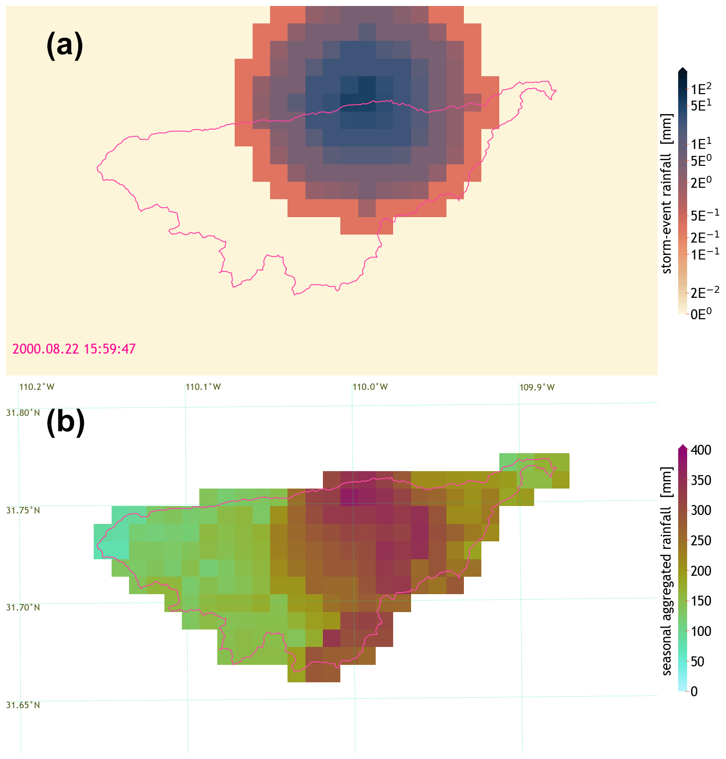
Figure 1 Spatiotemporal distribution of simulated storm rainfall over the WGEW (see Sect. 2.1). Spatial resolution of 1×1 km. (a) One large simulated storm starting at ∼ 16:00 MST on 22 August, with a radius of ∼7 km, ∼4.5 h duration, and a maximum intensity of ∼51.3 mm (i.e. 11.37 mm h⁻¹). Please note its logarithmic colour scale. (b) Cumulative seasonal distribution of 112 simulated storms for the wet season, i.e. from June through October. Even though the grid is presented in “lat–long” coordinates (i.e.  CRS WGS-84), the actual projection (in both panels) is the 2D Cartesian coordinate system known as NAD83/UTM zone 12N (i.e. EPSG:26912; https://epsg.io/26912, last access: 7 July 2024).

2.2 Total seasonal rainfall (TOTALP)

In order to remain faithful to the total seasonal rainfall distribution across a basin of interest, STORM stops a given simulation season once the median of the cumulative rainfall over the catchment surpasses the sampled TOTALP value for the season under consideration. The TOTALP value is sampled from a PDF of historical medians of total seasonal storm rainfall. Each of these historical medians represents the spatial median of the cumulative seasonal rainfall recorded by the gauge network spread within the catchment. To avoid sampling negative values of rainfall, the fitting (and the sampling) of the PDF is done in (natural) logarithmic space, i.e. $\text{TOTALP}=e^{{\text{TOTALP}}_{\text{(sampled)}}}$. Reaching the (catchment) median sampled from a distribution of historical medians offers a more accurate method for stochastic modelling of seasonal totals. Figure 1b shows the spatial distribution of rainfall at the end of one simulation run; i.e. once the median of the cumulative rainfall over the catchment is larger than the sampled value for TOTALP.

2.3 Maximum storm extent (RADIUS)

Storm radii are defined in STORM by grouping two or more gauges, computing the distance of each gauge to the centroid of the set/group of gauges, and selecting the maximum computed distance. Here, a “set/group of gauges” means all those gauges for which the time stamp of any storm start time is identically recorded among them in the historical database. A PDF of radii was generated from such groups with at least two rain gauges. We are aware that this assumption does not consider the extent, evolution, and/or trajectory of any storm in particular throughout the gauge data. Nevertheless, by assuming that identical time stamps in storm start times imply that the whole storm is being simultaneously captured by the gauge network, one can easily estimate an extension of the storm from gauge records. This premise also relies on the assumption of a circular-shaped model for storm cells and on a gauge network with consistent spatial density. Figure B1 shows the distribution of maximum storm (estimated) radii for the WGEW calibration dataset (i.e. storms recorded from August 1953 through October 1999; see Sect. 2.1). Figure 1a shows a simulated storm with a radius of ∼7 km. This approach is biased towards spatially large storms given that small-radii storms; i.e. storms not captured by a single gauge are disregarded in this methodology.

The minimum radius that can be sampled is restricted by the spatial resolution the user might set for the model output. For instance, for a model output resolution of 0.5×1.0 km, the minimum possible (sampled) radius would be 1 km. This is achieved by truncating the RADIUS PDF and then sampling from it. Instead of using a “maximum” criterion for the selection of storm radii, the user can also modify this criterion to be, e.g., the mean (or median or whatever) distance of a group of gauges and their centroid. This change can be implemented by the user via the pre_processing.py script. STORM 1.0 did not use a “radius” approach. Instead, storm area values were sampled from a pre-determined, fixed PDF.

2.4 Rainfall decay rate (BETPAR) and maximum storm intensity (MAXINT)

Following the approach of STORM 1.0, we model individual storms as isotropic circular cells, for which maximum intensities (I_max) are (always) located at their centres, with a quadratic exponential decay (β²) as the distance from such centres (r) increases:

$$\begin{array}{}\text{(1)}& I\left(r\right)=I_{\max }\cdot e^{-\mathrm{2}\cdot {\mathit{\beta }}^{\mathrm{2}}\cdot r^{\mathrm{2}}},\end{array}$$

where I(r) (in mm h⁻¹) is the rainfall intensity at a distance r (in km) from the storm centre. β has units of km⁻¹. We acknowledge that real storms may not be circular, but this assumption simplifies the mathematical representation of storms in the model.

In this new version, we use the quadratic exponential decay model to fit both the decay rate (β), and maximum intensity (I_max). This is done via scipy's module curve_fit; i.e. a non-linear least squares approach for which the trust region reflective method is applied, given the constraints we enforce to our minimization problem (Virtanen et al., 2020; Branch et al., 1999). Such constraints simply refer to the limits for which one intends β and I_max (in this case) to be within. For instance, and following Eagleson et al. (1987, Fig. 17), we bound β between zero and three, whereas we set I_max to be 3 times the highest intensity found in the gauge data as the upper limit and a value slightly above zero as the lower limit (0.07 mm h⁻¹ in our case). Morin et al. (2005) and Eagleson et al. (1987) previously used the same model to fit rainfall decay rate from radar and gauge data, respectively, for the WGEW. Figure 1a shows a simulated storm with a steep β of $\sim \mathrm{0.22}{\mathrm{km}}^{-\mathrm{1}}$ and $I_{\max }=\mathrm{11.4}\mathrm{mm}{\mathrm{h}}^{-\mathrm{1}}$.

We fit the model for storms simultaneously registered by four or more gauges (i.e. with identical starting time stamps). Along with the optimal values for which the model is fitted, curve_fit also returns the estimated covariance of such optimal values. We only kept optimal values for which their covariance is equal or smaller than 5 and equal to or larger than 0. These “clean” optimal values are the ones over which the PDFs (BETPAR and MAXINT) are then constructed. We obtained similar results (not shown here) to Morin et al. (2005) and Eagleson et al. (1987) for the PDF of β. In our case, β_mean≈0.1, compared to ∼0.4 for the Morin et al. (2005) and Eagleson et al. (1987) studies. This is mainly attributed to our methodology of simultaneously fitting both I_max and β. We also hit the μ≈0.4 when we only fit for β when using a larger number of storm records than they did in those previous studies.

We assume that in the vast majority of the cases, the rainfall recorded by the gauge network does not correspond to the maximum intensity of the storm event; thus, we required a method to model maximum storm intensity (MAXINT). Equation (1) is an adequate model that allows us to easily estimate the maximum rainfall intensity from gauge records (given the current computational tools and the extensive rainfall records). Figure B2 shows the difference between PDFs accounting (and not) for maximum intensity. Accounting for maximum storm rainfall intensity is a feature not present in STORM 1.0.

2.5 Storm average duration (AVGDUR)

The AVGDUR PDF is constructed from the corresponding optimal values for maximum intensity (MAXINT) (see Sect. 2.4). Once a “group of gauges” affected by a storm is established (see Sect. 2.3), storm duration is modelled as the average of all storm durations registered within this group. Nevertheless, the storm total duration registered by each gauge does differ from gauge to gauge, mainly due to the movement of the storm front over the gauge network. Thus, for every fit of Eq. (1) to a group of gauges (for which I_max and β are estimated), an average storm duration is also retrieved. And after selecting the best fits, with average storm durations included, we then proceed to fit the AVGDUR PDF.

2.6 Copula approach (MAXINT–AVGDUR COPULA)

The cornerstone of a copula framework is (set on) Sklar's theorem (e.g. Hofert et al., 2018, Chap. 1; Joe, 2014, Chap. 1; Nelsen, 2006, Chap. 2) which states that for any d-dimensional (joint) distribution function H with univariate marginals (margins) $F_{\mathrm{1}},\mathrm{\dots },F_d$, there exists a d-dimensional copula C such that

$$\begin{array}{}\text{(2)}& H\left(\mathit{x}\right)=C\left(F_{\mathrm{1}}\right(x_{\mathrm{1}}),\mathrm{\dots },F_d(x_d\left)\right),\mathit{x}\in {\mathbb{R}}^d.\end{array}$$

If the univariate marginals $F_{\mathrm{1}},\mathrm{\dots },F_d$ are continuous, then C is uniquely defined on [0,1]^d. In simpler terms, a copula is a function that links/couples (thus its etymology) a multi-variate (joint) distribution function to its univariate marginals with no prior knowledge of the actual shape (or type) of such marginals (e.g. Zhang and Singh, 2019; Hofert et al., 2018; Dai et al., 2014; Vandenberghe et al., 2011; Nelsen, 2006).

Elliptical copulas (which show elliptically contoured density level surfaces) refer to copulas from elliptical distributions (e.g. Tjøstheim et al., 2022, Chap. 5; Mai and Scherer, 2017, Chap. 4). An elliptical distribution represents a linear transformation of spherical distributions (Mai and Scherer, 2017, Chap. 4), with these being extensions of multi-normal distributions (Fang et al., 1990, Chap. 2). The vast majority of application from elliptical copulas are found in financial sciences (Genest et al., 2009; The Economist, 2009). Nonetheless, there are recent applications of elliptical copulas in hydrometeorology such as modelling radar rainfall uncertainty (Dai et al., 2014) and establishing the seasonal correlation between the El Niño–Southern Oscillation (ENSO), Pacific Decadal Oscillation (PDO), and precipitation (Khedun et al., 2014), for example. Chen and Guo (2019) and Zhang and Singh (2019) provide a thorough review of recent advances and applications of copulas (elliptical among others) in several areas of hydrology fields such as extreme analysis, drought(s), rainfall, flood (frequency, forecasting, and risk), streamflow, water quality, and suspended sediment transport. Elliptical copulas are very common and advantageous as they allow the specification of different levels of global correlation between marginals (Tjøstheim et al., 2022, Chap. 5). Nevertheless, they offer no simple closed-form expressions; that is, they have only implicit analytical expressions/solutions (Mai and Scherer, 2017, Chap. 4).

A (d-variate) Gaussian (i.e. standard normal) copula belongs to the parametric family of the elliptical copulas (e.g. Mai and Scherer, 2017, Fig. 4.1), and it is described by the functional form (e.g. Mai and Scherer, 2017, Chap. 4):

$$\begin{array}{}\text{(3)}& C_P^{\mathrm{Ga}}\left(\mathit{u}\right)={\mathbf{\Phi }}_P\left({\mathrm{\Phi }}^{-\mathrm{1}}\right(u_{\mathrm{1}}),\mathrm{\dots },{\mathrm{\Phi }}^{-\mathrm{1}}(u_d\left)\right),\end{array}$$

where Φ_P is the joint cumulative distribution function (CDF) of a d-variate Gaussian distribution; Φ⁻¹ is the univariate Gaussian inverse CDF (i.e. the quantile function); and P is the d×d correlation matrix of multi-variate normal random vector, with $C_P^{\mathrm{Ga}}$ denoting that the copula is parameterized by the $\frac{\mathrm{1}}{\mathrm{2}}d(d-\mathrm{1})$ parameters of the correlation matrix (McNeil et al., 2015, Chap. 7).

STORM uses a bi-variate Gaussian copula to model the dependence between storm rainfall intensity and duration. In a d-variate Gaussian copula, the d×d correlation matrix could be replaced by a/the covariance matrix (Mai and Scherer, 2017, Chap. 4). For the bi-variate case, i.e. d=2, $C_P^{\mathrm{Ga}}$ becomes $C_{\mathit{\rho }}^{\mathrm{Ga}}$, with ρ as the (scalar) Pearson correlation coefficient (e.g. Tjøstheim et al., 2022, Chap. 5; McNeil et al., 2015, Chap. 7; Joe, 2014, Chap. 4). In doing so, the parameterization is reduced to its minimum (only dependent on ρ), allowing its (relatively) easy implementation and therefore its popularity. Still, a bi-variate (or any d variate, for that matter) Gauss copula does not have a simple closed form but can be expressed as an integral over the density of a bi-variate normal random vector (e.g. McNeil et al., 2015, Chap. 7; Ross, 2013, Chap. 6):

$$\begin{array}{}\text{(4)}& \begin{array}{rl}{C}_{\mathit{\rho }}^{\mathrm{Ga}}(u,v)& =\underset{-\mathrm{\infty }}{\overset{{\mathrm{\Phi }}^{-\mathrm{1}}\left(u\right)}{\int }}\underset{-\mathrm{\infty }}{\overset{{\mathrm{\Phi }}^{-\mathrm{1}}\left(v\right)}{\int }}{\displaystyle \frac{\mathrm{1}}{\mathrm{2}\mathit{\pi }\sqrt{\mathrm{1}-{\mathit{\rho }}^{\mathrm{2}}}}}\\ & \cdot \text{exp}\mathit{\{}-{\displaystyle \frac{u^{\mathrm{2}}+v^{\mathrm{2}}-\mathrm{2}\mathit{\rho }uv}{\mathrm{2}(\mathrm{1}-{\mathit{\rho }}^{\mathrm{2}})}}\mathit{\}}\mathrm{d}v\mathrm{d}u,\\ & \text{with}\mathrm{0}⩽u,v⩽\mathrm{1},\text{and}\mathit{\rho }\in [-\mathrm{1},\mathrm{1}].\end{array}\end{array}$$

STORM constructs the bi-variate Gaussian copula via the GaussianCopula module from the statsmodels package (Joe, 2014; Seabold and Perktold, 2010). First, during the pre-processing stage (Sect. 2.9), the Pearson correlation coefficient ρ is obtained through Greiner's equality (Berger, 2016):

$$\begin{array}{}\text{(5)}& \mathit{\tau }={\displaystyle \frac{\mathrm{2}}{\mathit{\pi }}}\cdot \text{arcsin}\left(\mathit{\rho }\right),\end{array}$$

where τ is Kendall's rank correlation (also known as Kendall's tau) (Virtanen et al., 2020; Kendall, 1945). A rank correlation is a copula-based measure of the (strength of the) dependence; i.e. it only depends on the copula (of a bi-variate distribution) and not on the marginals (McNeil et al., 2015, Chap. 7). It is computed from the ranks of the (empirical) data, which means one only needs the ordering of the random variables and not the actual values, i.e. storm intensity and duration in this case. Equation (5) generally holds for elliptical copulas (from which the bi-variate Gaussian is a member), offering a simple approach to compute ρ without the estimation of variances and covariances (Langworthy et al., 2021; McNeil et al., 2015, Chap. 6). Then, during a simulation (or validation) run, the bi-variate normal distribution is constructed from Eqs. (5) and (4) using the probability integral transform (Seabold and Perktold, 2010). Once the (bi-variate) Gaussian copula is built, n samples are randomly sampled from it. These samples are drawn from the $\mathrm{0}⩽u,v⩽\mathrm{1}$ CDF space; hence, each sample, i.e. (u,v) point, must be transformed (back) into the intensity–duration space. This transformation is done throughout the marginal PDFs (and their ppf objects from scipy's module stats). During the pre-processing stage, STORM builds the marginal PDFs for intensity and duration from the input gauge data.

Figure 2 shows a comparison between storm rainfall measured by rain gauges and simulated from a bi-variate Gaussian copula. From this figure, one can see that for the simulated exercise (Fig. 2b), STORM generates storms with higher (and lower) intensities than those actually observed by the gauge network (Fig. 2a), supporting a wider distribution of potential storm characteristics.

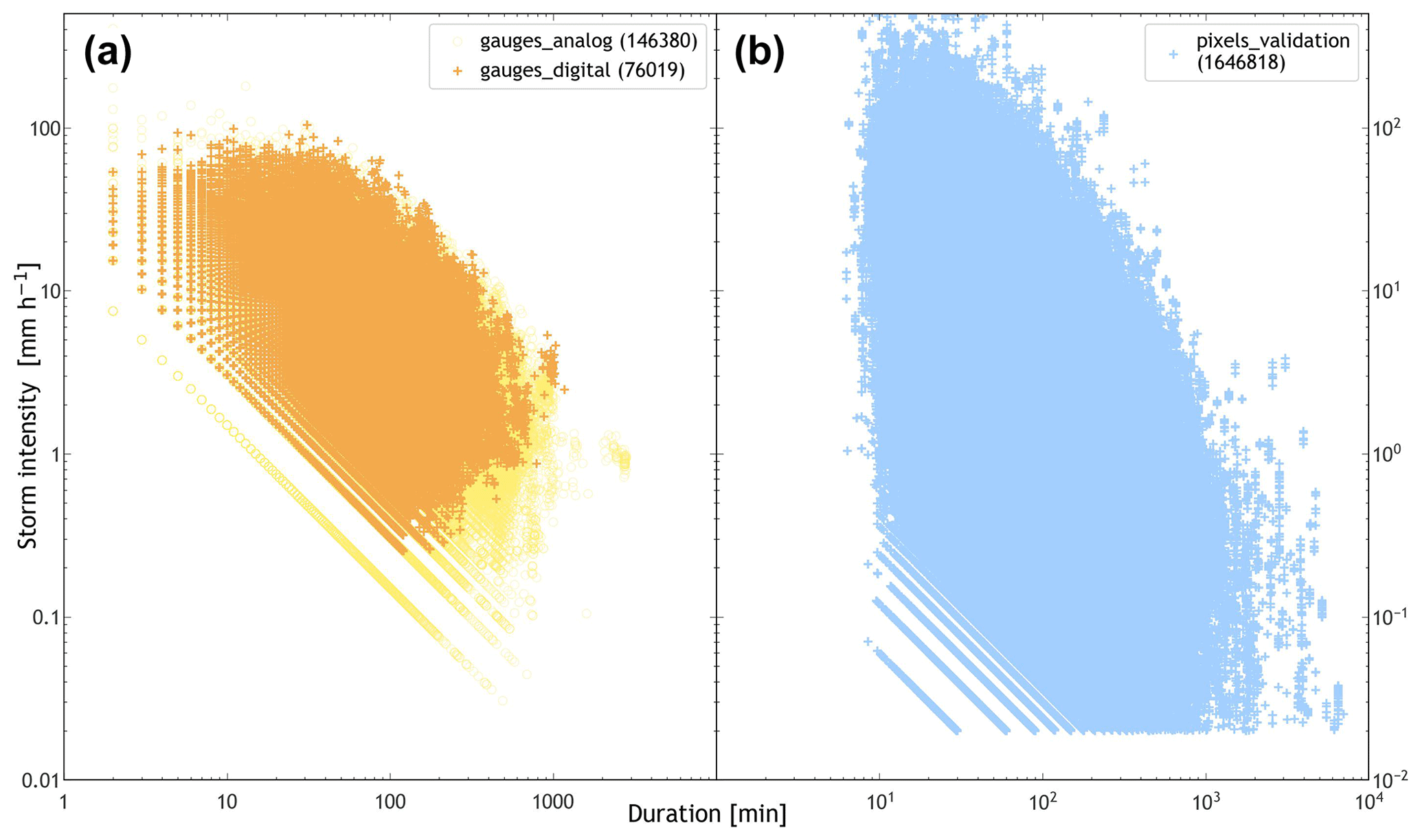
Figure 2 Scatter plots of storm intensity (y axis; mm h⁻¹) against storm duration (x axis; min) in log–log scale for gauge and validation datasets. (a) Recorded storms for the wet season (i.e. June through October) over the WGEW (see Sect. 2.1). The orange markers/crosses are records from the digital network, i.e. gauges from 2000 onwards (from June 2000 through October 2022; i.e. the validation dataset). The yellow markers/circles are records from the analogue network, i.e. gauges prior to 2000 (from August 1953 through October 1999; i.e. the calibration dataset). (b) The 23 years of simulated storms, with each year having 30 runs. These storm intensity–duration “pairs” are obtained from the marginal PDFs fitted in the pre-processing module (see Sect. 2.9) for storm maximum intensity (MAXINT) and average duration (AVGDUR), after being randomly sampled (in the $\mathrm{0}⩽u,v⩽\mathrm{1}$ CDF-space) from a bi-variate Gaussian copula (Eq. 4) with $\mathit{\rho }=-\mathrm{0.31622}$.

2.7 Day of year (DOYEAR) and time of day (DATIME)

Realistic storm start dates and times can now be sampled in STORM through a modular implementation of directional (or circular) statistics. Directional statistics take into consideration the periodicity of random variables that can be distributed in a closed space, e.g. torus, sphere, and circle (Breitenberger, 1963). The day of the year (DOY) and the time of the day (TOD) of an occurring storm belong to such a set of variables. This innovation supports the analysis of how rainfall accumulates throughout a season and how rainfall timing might be biased by the diurnal cycle (e.g. afternoon rainfall occurrence due to convective heating of the land surface).

STORM models storm start dates and times throughout a finite mixture of unimodal von Mises (vM) distributions. The vM distribution (also known as the Tikhonov distribution; e.g.  Shmaliy, 2005) is a widely used PDF (in the circle space) given its simplistic parameterization and mathematical tractability (e.g. Pewsey et al., 2013; Mardia and Jupp, 1999). The vM distribution is a close approximation of distributions such as the cardioid, the wrapped Cauchy, and the wrapped normal. This latter distribution (as its name suggests) is the equivalent of wrapping the normal distribution (from the linear space) into the circular space (Mardia and Jupp, 1999, Chap. 3).

The model for a finite mixture of vM (MvM) PDFs (for a random variable θ) is given by (e.g. Jammalamadaka and SenGupta, 2001, Chap. 4.3)

$$\begin{array}{}\text{(6)}& f\left(\mathit{\theta }\right|\mathit{\{}p,\mathit{\mu },\mathit{\kappa }{\mathit{\}}}_{i=\mathrm{1}}^{\text{M}})=\sum _{i=\mathrm{1}}^{\text{M}}{p}_i\cdot {\displaystyle \frac{e^{{\mathit{\kappa }}_i\cdot \text{cos}(\mathit{\theta }-{\mathit{\mu }}_i)}}{\mathrm{2}\mathit{\pi }\cdot I_{\mathrm{0}}\left({\mathit{\kappa }}_i\right)}},\end{array}$$

with 0⩽θ, μ_i<2π, $\mathrm{0}⩽p_i⩽\mathrm{1}$, and ${\sum }_{i=\mathrm{1}}{p}_i=\mathrm{1}$.

In Eq. (6), p_i is the mixing proportion of the i unimodal vM distribution (i.e. everything to the right of p_i), κ for κ⩾0} is the concentration parameter that quantifies the sparseness/spreading of the distribution around its mean direction μ and I₀(κ) is the modified Bessel function of the first kind with order 0 and argument κ. Jammalamadaka and SenGupta (2001, Eq. 2.2.7) and/or Mardia and Jupp (1999, Eq. 3.5.19), for instance, define I₀(κ) as

$$\begin{array}{}\text{(7)}& I_{\mathrm{0}}\left(\mathit{\kappa }\right)={\displaystyle \frac{\mathrm{1}}{\mathrm{2}\mathit{\pi }}}\underset{\mathrm{0}}{\overset{\mathrm{2}\mathit{\pi }}{\int }}{e}^{\mathit{\kappa }\cdot \text{cos}\left(\mathit{\theta }\right)}\mathrm{d}\mathit{\theta }=\sum _{s=\mathrm{0}}^{\mathrm{\infty }}{\displaystyle \frac{\mathrm{1}}{(s\mathrm{!}{)}^{\mathrm{2}}}}({\displaystyle \frac{\mathit{\kappa }}{\mathrm{2}}}{)}^{\mathrm{2}\cdot s}.\end{array}$$

This latter, i.e. the rightmost term in Eq. (7), is the power series expansion (in infinite series form). Parameters μ and $\mathrm{1}/\mathit{\kappa }$ (Eq. 6) are analogous to the mean μ and variance σ² of the normal distribution.

Equation (6) has no analytical solution. Hence, STORM uses the vonMisesMixtures (https://framagit.org/fraschelle/mixture-of-von-mises-distributions, last access: 7 July 2024) package, which computes the parameters (μ, κ, p) via maximum likelihood estimators within an expectation–maximization framework (e.g. Hornik and Grün, 2013; Dhillon and Sra, 2003). The description of such an algorithm is beyond the scope of this work. At its core, the vonMisesMixtures package uses the iv object from scipy's module special for the modified Bessel function (Virtanen et al., 2020; Temme, 1975) and the fsolve object from scipy's module optimize for the root finding (of non-linear functions). fsolve, ultimately, is a wrapper for a modified Powell's hybrid method (Moré et al., 1980, p. 57–64, 71–78); this latter method is an algorithm for non-linear optimization (Powell, 2009, 1970).

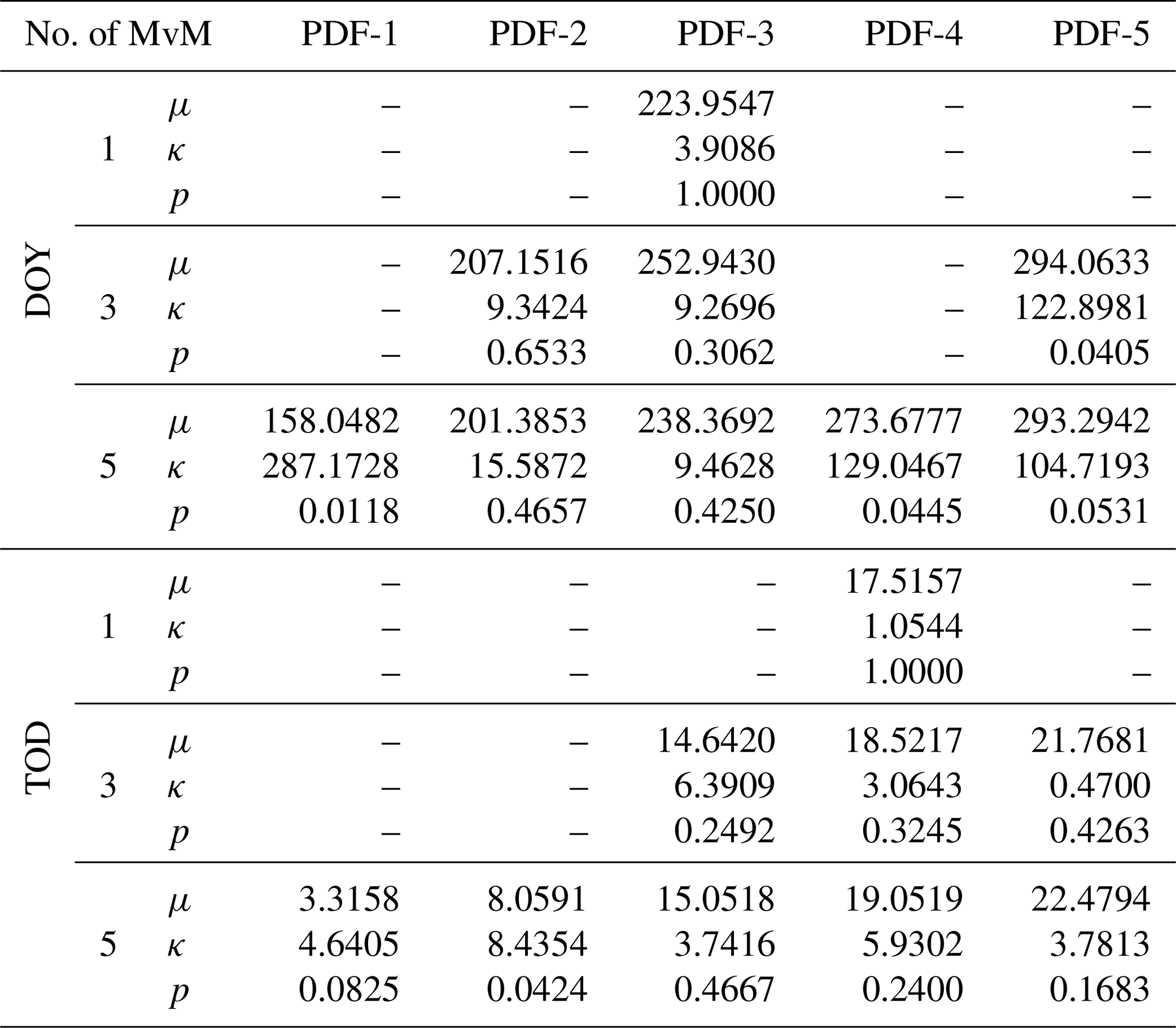
Table 1 presents the estimated parameters for mixtures of one, three, and five vM PDFs. Given the storm start DOY and TOD, STORM transforms those date and time stamps into radians and feeds them to the vonMisesMixtures package, along with the number of vM PDFs to compute the mixture. The conversion from decimal-based days (d_dec) into radians (d_rad), follows: $d_{\mathrm{rad}}=\mathit{\pi }(\mathrm{2}\cdot d_{\mathrm{dec}}/\mathrm{365}-\mathrm{1})$ for $\mathrm{0}⩽d_{\mathrm{dec}}⩽\mathrm{365}$, and $-\mathit{\pi }⩽d_{\mathrm{rad}}⩽+\mathit{\pi }$. Similarly, the conversion from decimal-based hours (h_dec) into radians (h_rad), follows: $h_{\mathrm{rad}}=\mathit{\pi }(h_{\mathrm{dec}}/\mathrm{12}-\mathrm{1})$ for $\mathrm{0}⩽h_{\mathrm{dec}}⩽\mathrm{24}$, and $-\mathit{\pi }⩽h_{\mathrm{rad}}⩽+\mathit{\pi }$. Figure 3 shows the fitted mixtures reconstructed from the parameters in Table 1, along with the circular distribution of DOY and TOD. In Fig. 3b, the optimal (and more parsimonious) fit for TOD is given by three MvM PDFs. A fit for five MvM PDFs is also presented in Fig. 3b, even though it is overshadowed by the three MvM PDFs. This shows the preference (and optimality) of the latter model not only for capturing in detail the (potential) multi-modality of the TOD distribution (e.g. afternoon and nighttime storms being the most common between June and October) but also offering a less burdensome/intensive parameter estimation with regard to the former model (i.e. five MvM PDFs). Disregarding its circular framework, the TOD histogram presented in Fig. 3 is consistent with that of Eagleson et al. (1987, Fig. 5). Appendix A presents the rationale behind the optimum selection of five MvM PDFs for DOY, and three MvM PDFs for TOD, which are the default settings in STORM. Still, we encourage the user to assess the optimal number of vM PDFs on a case-by-case basis.

Figure 3 (a) Circular distribution for 3 d binned data of (storm start) days of year (DOY; orange dots, with each dot representing 350 counts). The continuous black curve indicates the optimal mixture of von Mises (MvM) probability density functions (PDFs), which is a mixture of five vM PDFs, in this case (see Appendix A). The green curve represents a fit for three MvM PDFs. A 5 d bin circular histogram is also plotted on the inside. (b) Circular distribution for 12 min binned data of (storm start) times of day (TOD; blue dots, with each dot representing 150 counts). The continuous red curve indicates the optimal MvM PDFs, i.e. three MvM PDFs, in this case. The (almost imperceptible) green curve represents a fit for five MvM PDFs. A 1 h bin circular histogram is plotted on the inside. In both panels, the dashed black curves represent a fit of just one vM PDF. The size of the sample is ∼146k values for both DOY and TOD, encompassing the wet seasons (June through October) from 1953 through 1999, in the WGEW (see Sect. 2.1). Table 1 (Sect. 2.7) displays the parameters μ, κ, and p which the vM PDFs are constructed from.

The choice to implement an approach like the MvM PDFs allows the end-user to account for potential multi-modality (and asymmetry) in their storm start date and times. Nonetheless, in the eventuality that any user encounters some difficulties when installing or running the vonMisesMixtures package (as it is not shipped through the conda channels (Anaconda Software Distribution, 2023)), or that they simply do not want to follow such an approach, STORM can still run without this feature (once it is turned off). In that case, STORM finds the best fit throughout a set of discrete probability mass functions (PMFs) for the DOY and samples TOD from a uniform distribution (upscaled to the 00:00–24:00 h domain). Figure B3 shows the best fit of a PMF for DOY in the WGEW dataset. In Fig. B3, one can see the advantages of using a more elaborate model. i.e. MvM PDFs, with regard to a simple PMF model. Having a statistical model for the DOY is another improvement over STORM 1.0. Thus, we avoid modelling inter-arrival and do not contradict the notion of rainfall modelling from a (Poisson) point process perspective (e.g. Eagleson et al., 1987).

Both TOD and DOY sampling take place independently from one another. Then, they are glued together into full date and time stamps (i.e. DOYEAR and DATIME).Although theoretically possible, the probability of having two storms simulated at the same location with the very same date and time stamp is extremely low.

Table 1 Mean dates and times μ (in decimal days of year for DOY and in decimal hours for TOD, respectively), concentration parameters κ, and mixing proportions p for one, three, and five mixtures of von Mises (MvM) probability density functions (PDFs). For instance, for the time of day (TOD) and for the three MvM PDFs, μ (in radians) are 0.691, 1.707, and 2.557, i.e. (in decimal hours), 14.64, 18.52, and 21.77 (where 0_rad=12:00 and $-\mathit{\pi }/+\mathit{\pi }=\mathrm{00}$:00/24:00). The parameters for the five and three MvM PDFs are, respectively, the default for the DOY and TOD models in STORM. These defaults are defined in the pre_processing.py script/module (and in the input file ProbabilityDensityFunctions_ONE–ANALOG.csv). The fitted PDFs presented in Fig. 3 (and Fig. B3) can be reconstructed by plugging these parameters into Eqs. (7) and (6).

2.8 Scaling factors and orographic stratification

One key feature carried on from its predecessor is STORM's capability to model potential future climate change scenarios throughout two scaling factors (f₁,f₂) applied to TOTALP (total seasonal rainfall) and MAXINT (maximum storm intensity). Equation (8) is a generic equation in which U represents the variable to be scaled (i.e. TOTALP or MAXINT), U^* is its new value after being modified by factors f₁ or f₂, and k is the iterator for the number of years per simulation, namely NUMSIMYRS.

$$\begin{array}{}\text{(8)}& U^{*}=U\cdot (\mathrm{1}+f_{\mathrm{1}}+(f_{\mathrm{2}}\cdot k\left)\right),\mathrm{0}<k⩽\text{NUMSIMYRS}\end{array}$$

Equation (8) implies that for every simulated year one can apply either a factor f₁, which yields a constant increase (or decrease) for every year throughout the whole span of the simulation, or a factor f₂ which progressively increases (or decreases) with regard to the previous simulated year. For instance, a factor $f_{\mathrm{1}}=-\mathrm{0.1}$ will decrease by 10 % every sampled TOTALP in any given n-year simulation, indicating a progressively drying climate, whereas a factor $f_{\mathrm{2}}=+\mathrm{0.1}$ will double the value of sampled TOTALP at the end of a 10-year simulation, characterizing a climate that is getting wetter, for instance. Both factors (f₁,f₂) are expressed as percentages and are mutually exclusive; i.e. STORM ensures they cannot be applied at the same time, even though Eq. (8) suggests the opposite (this constraint can easily be removed from the source code, though). Otherwise, the effect of each factor in the output becomes somewhat challenging to disentangle.

For TOTALP, f₁=PTOT_SC, and f₂=PTOT_SF, whereas for MAXINT, f₁=STORMINESS_SC, and f₂=STORMINESS_SF (i.e. variables used in the script rainfall.py). A legacy from STORM 1.0, PTOT_SC, is a factor that simulates (percentage) step changes in the catchment wetness (seasonal precipitation totals), whereas PTOT_SF is a fractional scaling factor (progressive percentage) that simulates temporal trends in seasonal totals. Similarly, STORMINESS_SC simulates step changes in storminess (increase/decrease in maximum storm intensities), whereas STORMINESS_SF is a fractional scaling trend in maximum intensities. Section 3.2 shows the results for one simulation where $\text{PTOT\_SC}=+\mathrm{0.5}$ (Figs. 8 and B7b) and another where $\text{STORMINESS\_SF}=-\mathrm{0.035}$ (Figs. 7 and B7a).

STORM now offers the possibility for the simulation of storm rainfall (e.g. intensity and duration) at different elevation bands, so orographic effects are taken into account. The basic (and simplest) set-up of STORM only requires the catchment shapefile (SHP) to determine the spatial domain over which the simulation(s) will take place. In this is scenario, it is not possible to determine any elevation bands from the SHP, and STORM reverts back to sampling storm intensity–duration pairs from the “global” copula; i.e. the copula model retrieved from all gauge data (see Sect. 2.6 and Fig. 2). On the other hand, if the user provides a SHP and its digital elevation model (DEM), then STORM can compute as many copulas as there are elevation bands into which the catchment is split (e.g. based on hypsometric analysis). To this end, and during the pre-processing stage (see Sect. 2.9.1), the user must define such elevation bands, and STORM will compute one copula per elevation band (as long as the storm/gauge dataset also provides the elevation of the gauge network, which is almost always the case). During the simulation/validation stage, the extent of the storm is defined and overlapped to the DEM, and then STORM calculates the median elevation, which is ultimately used to infer which copula (band) maximum rainfall intensity must be sampled from. By default, STORM calculates the median elevation of the storm extent over the DEM. Nevertheless, this metric can be changed to another statistic, for instance, the mean (see Sect. 2.9.1). Figure B5 shows the capability of STORM to account for orography, in this case, the simulation of different sets of storms at three elevation bands, e.g. up to 1350, between 1350 and 1500, and above 1500 m a.s.l. (metres above sea level). We found no significant differences in simulated or measured storms among any of these three bands, which can be attributed to the low orographic gradient within the WGEW.

2.9 Extras

2.9.1 Pre-processing module

This module is divided in two parts: (1) the actual module that processes all gauge data and generates the PDFs that STORM uses as input and (2) the file parameters.py in which all “soft-” and “hard-coded” parameters/variables are placed and can be read/ingested by STORM.

Table 2 The first and last four rows of the (sorted) storm-event-based gauge data used by the script pre_processing.py to compute the best-fit parameters presented in Table 4. In the S column, W indicates a storm occurring within the established wet season. The complete table/data can be found in the file gage_data–1953Aug18-1999Dec29_eventh–ANALOG.csv that is located in the folder/path model_input/data_WG.

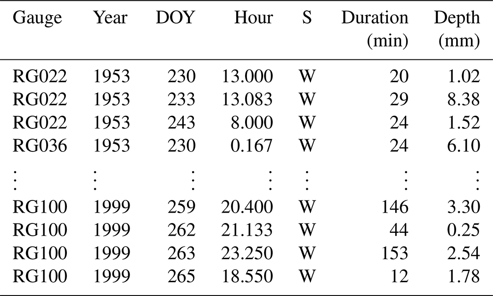
The standalone script pre_processing.py ingests event- and aggregate-based gauge data to best-fit PDFs for several variables (see Tables 2 and 3). These storm variables are as follows:

• total seasonal rainfall – TOTALP,

• maximum extent – RADIUS,

• rainfall decay rate – BETPAR,

• maximum intensity – MAXINT,

• average duration – AVGDUR,

• intensity–duration copula – COPULA,

• starting date – DOYEAR, and

• starting time – DATETIME.

The best-fitted PDFs are generated through Python's library fitter (Cokelaer et al., 2023). For a given variable/parameter, STORM's pre-processing module passes post-processed data to fitter, along with several families of probability distributions that might be adequate for its fitting. At its core, fitter uses scipy's object fit (from the stats module; see Sect. 2.6) “to extract the parameters of that distribution that best fit the data”. This is done via either the maximum likelihood estimation method or the method of moments (Virtanen et al., 2020). Because several probability distributions are passed to fitter (distributions which users can modify according to their needs), the latter finds the best-fitted parameters for such distributions and computes several assessment metrics, including the error sum of squares (SSE), AIC (Akaike's information criterion), and BIC (Bayesian information criterion; see Appendix A). The pre-processing module selects the fitted PDF with the lowest BIC (this assessment metric can be modified too by the user). The impact of parameter misspecification and estimation error and/or uncertainty in the performance of STORM is also beyond the scope of the present work. Tools like fitter are practical implementations that ultimately reduce to a minimum these sort of potential impacts in STORM's performance/outcomes.

Table 3 Only 12 rows of the storm-aggregated gauge data used by the script pre_processing.py to compute the best fit for total seasonal rainfall (TOTALP in Table 4). In the S column, W indicates a month within the established wet season, whereas D is for months out of such a wet season. The complete table/data can be found in the file gage_data–1953Aug-1999Dec_aggregateh–ANALOG.csv that is located in the folder/path model_input/data_WG.

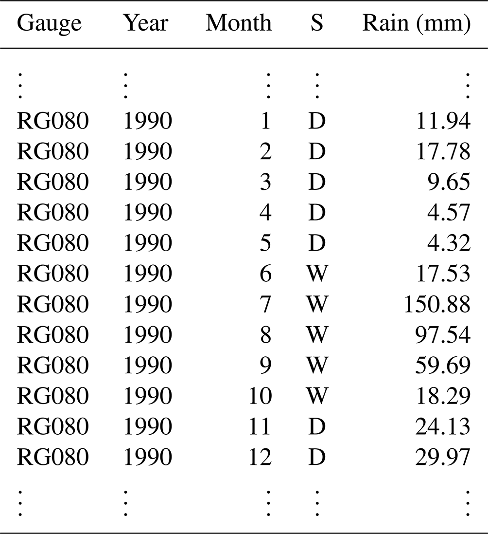
Table 4 Parameters of PDFs that best fit the WGEW gauge data for a given random variable. _PDF indicates probability density functions, _RHO refers to the copula ρ parameter, and _VMF indicates a von Mises PDF. The number next to the aforementioned nomenclature refers to the wet season for which the variable is estimated/fit. In this case, there is only one wet season, thus the number 1. The “Z#” tag refers to the elevation band for which the parameters (of the random variable) are estimated. If the variable does not present such a tag (i.e. rows 1–5, 12, and 16–23), then that means that the parameters were estimated/fit regardless of elevation. Except for COPULA, DATIME, and DOYEAR, the end-string indicates the PDF family to which the parameters belong so that STORM (via scipy) can construct the adequate PDF. For variables built upon PDFs, i.e. rows 1–11, par-1 and par-2 columns are, respectively, for the mean and the variance. If the PDF presents more than two parameters (i.e. par-3 and/or par-4), then they are for location and scale. For COPULA, par-1 represents the correlation parameter ρ (see Sect. 2.6). For DOYEAR and DATIME, “m#” indicates the number of vM PDFs that make up the mixture, i.e. five vM for DOYEAR (see Sect. 2.7) and three vM for DATIME. Columns par-1, par-2, and par-3, respectively, represent their p, μ (in radians), κ parameters (see Table 1). This table is produced by the script pre_processing.py, exported as ProbabilityDensityFunctions_ONE–ANALOG.csv into the model_input folder/path, and later ingested by STORM.

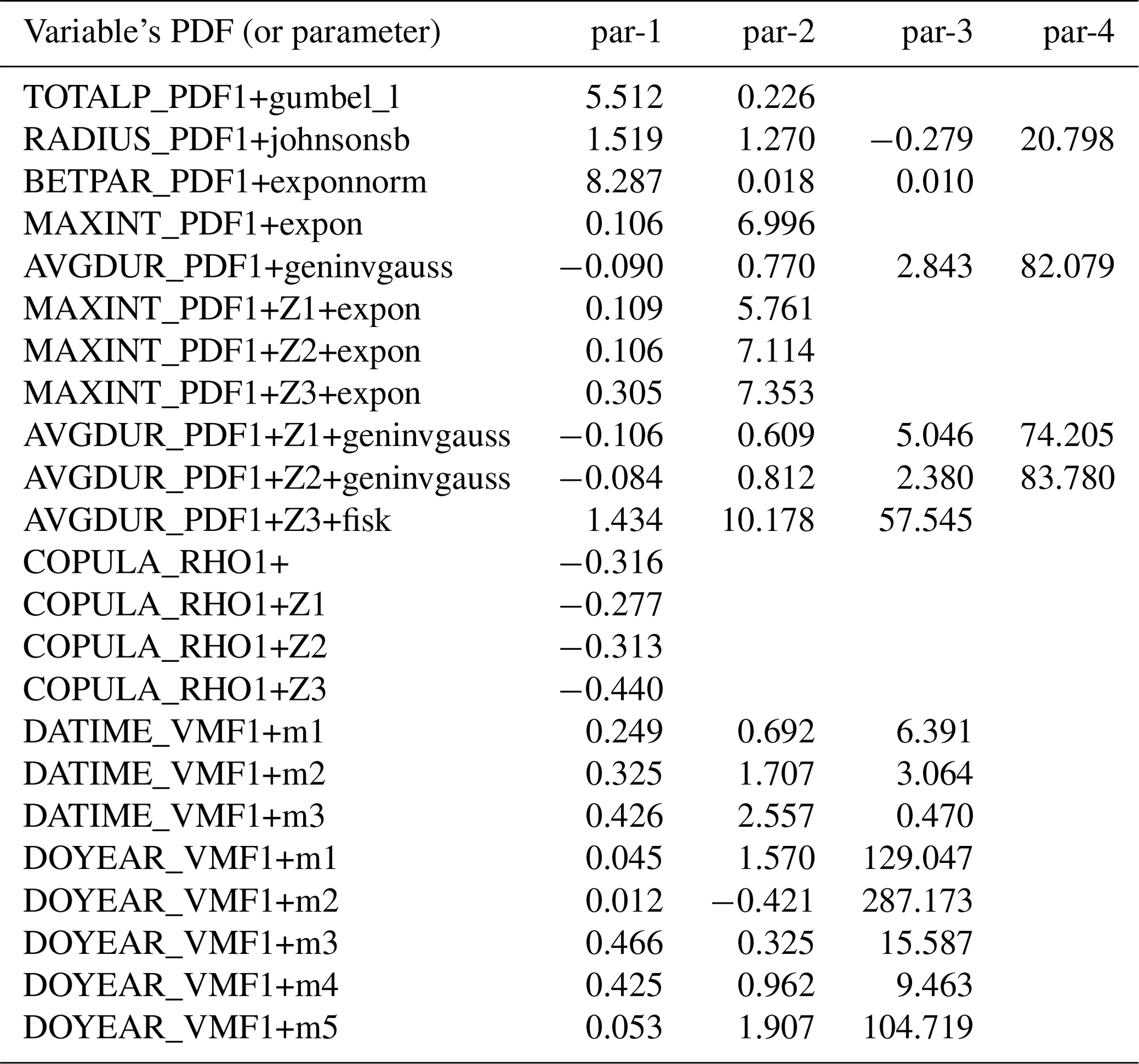
After the PDF fitting and selection is done, the best-fitted PDF parameters are then exported to a CSV (comma-separated value) file (stored in the model_input/data_WG folder) that is later read during the simulation/validation stage. Appending the tags “_PDF” (probability density function), “_RHO” (copula ρ parameter), and “_VMF” (von Mises PDF) allows STORM to read all the necessary statistical parameters stored in one single file (see Table 4). The number 1 appended to the PDF, RHO, and VMF tags indicates that the preprocessing was done for only one wet season. If analyses are carried out for more than one wet season, then STORM replicates the same analyses for every season, appending numerical tags accordingly (e.g. file ProbabilityDensityFunctions TWO-ANALOG-py.csv). If the analysis requires elevation stratification, STORM generates MAXINT and AVGDUR PDFs for each elevation band and appends a “Z#” tag to distinguish them from the all-gauge-based PDFs (see Table 4; rows 6–11 and 13–15). For the directional/circular variables DOYEAR and DATETIME, STORM appends as many “m#” tags as the number of vM PDFs required for the given mixture (see Table 4; last eight rows).

2.9.2 Visualization tool

GIF (graphics interchange format)³ animations of selected simulations are created via the script animation.py (located in STORM's xtras folder/path). STORM's simulations (or validations) are stored in NetCDF (Network Common Data Form)⁴ files; i.e. one file per each season containing m simulations for each 1 of n years. Once the NetCDF files are produced for a given simulation/validation, the user can easily create animations (and/or snapshots) depicting the evolution of storm events during the wet season, along with its seasonal aggregation within the defined catchment. An example of such an animation can be found in the README.md (page) of STORM's repository (https://github.com/feliperiosg/STORM2, last access: 7 July 2024). The snapshots from which the animation is built look like Fig. 1.

2.10 STORM's skeleton

Starting from the pre-processing module (see Algorithm 1), STORM ingests pre-preprocessed storm data in the format presented in Tables 2 and 3. The output of this pre-processing module is the file ProbabilityDensityFunctions_ONE–ANALOG.csv, which contains the parameters of several PDFs needed to stochastically model rainfall storms. Table 4 presents the aforementioned file in its entirety.

Algorithm 2 is the cornerstone of STORM. This algorithm shows the main steps required to simulate storm rainfall and relates all the stochastic variables previously described. Algorithm 3 (script storm.py) is the wrapper responsible for (1) gathering the input files/parameters (scripts parameters.py and parse_input.py), (2) verifying that all the necessary file/parameters and variables are correctly set and allocated (script check_input.py), and (3) ultimately calling Algorithm 2 (i.e. script rainfall.py).

Algorithm 1 Pre-processing module.

create CSV file {all the processes below write into this file}

read (pre-processed) gauge data and metadata

fit (wet) seasonal PDF

estimate and fit radii PDF

estimate and fit rainfall decay rate and maxima intensity

compute intensity–duration copula {with stratification or not}

compute and fit DOY and TOD PDFs

Algorithm 2 Computes and exports storm rainfall.

for i⩽SEASONS do

create NetCDF file

for j⩽NUMSIMS do

for k⩽NUMSIMYRS do

TOTALP ← sample total seasonal rainfall

TOTALP $\leftarrow \text{TOTALP}\cdot (\mathrm{1}+f_{\mathrm{1}}+f_{\mathrm{2}}\cdot k))$

$\text{NUM\_S}\leftarrow \mathrm{40}*\mathrm{5}$ {initial number of storms}

CUM_S←0 {initial cumulative rainfall}

while $\text{CUM\_S}<\text{TOTALP}\wedge \text{NUM\_S}⩾\mathrm{2}$ do

CENTERS ← sample centre geolocations

BETPAR ← sample rainfall decay rates

RADIUS ← truncated sampling of radii

stratification {if requested}

MAXINT, AVGDUR ← copula sampling

MAXINT $\leftarrow \text{MAXINT}\cdot (\mathrm{1}+f_{\mathrm{1}}+f_{\mathrm{2}}\cdot k))$

DOYEAR, DATIME ← sample of date and time stamps

rasterisation

interpolation

aggregation {CUM_S updated}

NUM_S $\leftarrow \text{NUM\_S}/\mathrm{2}$

end while

write into NetCDF file

end for

end for

close NetCDF file

end for

Algorithm 3 STORM in a nutshell.

Require:

input parameters {passed to the shell or read from a file}

Ensure:

input parameters make sense

call Algorithm 2 {simulates rainfall}

3 Results and discussion

3.1 Evaluation of STORM

We carried out a validation run to evaluate the performance of STORM. In STORM, a “validation” run is equivalent to a “simulation” run (thus, we use these terms interchangeably). The difference is that for a simulation run the catchment mask is exported along with the output file, whereas for the validation run the mask of the gauge network (for which the validation exercise is carried out) is the one stored in the output. We ran 30 simulation runs, each comprising 23 years, through STORM. The above is equivalent to having $\sim \mathrm{1.65}\times {\mathrm{10}}^{\mathrm{6}}$ storms, compared against the ∼76 000 storms (for the wet season) measured by the automatic network from 2000 through 2022, i.e. the validation dataset.

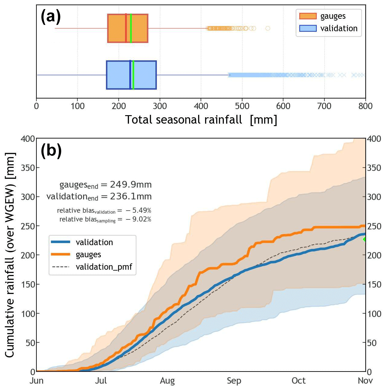
Figure 4 (a) Distribution of storm rainfall totals (for the wet season) year-by-year and station/pixel-based, i.e. not spatially averaged, over the catchment. Blue represents the validation dataset (∼50.6k samples), whereas orange is for the gauge dataset (∼1.9k samples). The bright green line (inside the boxplots) represents the mean of the distribution, i.e. 229.2 mm and 235.4 mm, respectively, for gauge and validation sets. (b) Percentile time series for the 90th percentile of all time series from June through October (wet season) for the validation (blue) and gauge (orange) datasets. The solid lines represent the median(s) of each dataset (50th percentile). The dashed black line represents the median for a validation where DOY was modelled through a discrete PMF (see Fig. B3). The green marker at the end of the time series indicates the median of the sampled (simulated) values of total seasonal rainfall (TOTALP). Figure B4 shows percentile time series for the 100th percentile.

In general terms, STORM does well what it was set up to do, i.e. to reach the median precipitation over the entire catchment. This can be seen from the boxplots presented in Fig. 4a, where the (pixel/gauge aggregated) median for the validation dataset (228.3 mm) is just 5 % larger than the median for the gauge data (217.4 mm). This difference is mainly due to STORM always stopping after the (sampled) median seasonal total (TOTALP) is reached. Therefore, STORM seasonal aggregates (on average) will always be larger than the sampled value of reference. One advantage of such a stochastic approach is the ability to reach maxima (and minima) seasonal totals (per station/pixel) outside the inter-quartile range of the gauge dataset, thus accounting for unrecorded (but potential) extreme events.

Due to the introduction of a new statistical characterization of the storm start date and time (DOY and TOD), STORM now captures some of the intra-seasonal variability in the rainfall. This can be seen in the percentile time series of cumulative seasonal rainfall presented in Fig. 4b. This latter plot shows how (on average) the cumulative rainfall, over the WGEW, slowly rises to a peak (inflexion point in the solid orange line) halfway through the wet season, from which then follows a slow and steady decline until November. Such a seasonal intra-variability is replicated by STORM (solid blue line) having a final underestimation of 5.5 % (i.e. 236.1 mm) with regard to the actual seasonal (cumulative) median of 249.9 mm. In the case that any user does not follow the circular statistics approach (see Sect. 2.7), STORM does also replicate rainfall intra-seasonal variability using a discrete PMF (dashed black line in Fig. 4b). However, it should be emphasized that STORM does not represent other local hydrometeorological patterns and global teleconnections (e.g. Sarachik and Cane, 2010; Diaz and Markgraf, 2000; Philander, 1990) that might contribute to intra- and inter-seasonal rainfall variability. The modelling of teleconnection phenomena/patterns in STORM was beyond the scope of this work. Nevertheless, such patterns could be empirically represented for particular seasons by altering either the rainfall total PDF (TOTALP) or maximum storm intensity (MAXINT), respectively, via the scaling factors PTOT_ or STORMINESS_ (see Sect. 2.8). For a control run, i.e. one without climate drivers (see Sect. 3.2), the scatter plot presented in Fig. 5 shows STORM's inability to depict extreme stormy seasons either wetter or drier than those in the historical distribution (i.e. a very low coefficient of determination; ρ²=0.0028). For instance, gauge data tell us that the years 2022 and 2020 had the wettest and driest seasons of the last 2 decades, respectively. The seasonal averages (for the whole gauge network) were 429.9 mm for 2022 and 82.5 mm for 2020. These seasonal (mean) extremes contrast with the systematic simulations (30 runs for each year) for which the validation dataset averages 237.0 mm for 2022 and 222.2 for 2020. Nonetheless, and regardless of the intra- and inter-annual rainfall variabilities, the seasonal average pixel total (235.4 mm) is just 3.2% larger than the seasonal average gauge total (228.1 mm). Having a low (auto-)correlation is not considered a bad feature in STORM and other stochastic models. As suggested and demonstrated by, e.g., Kim et al. (2017), a model performing better in metrics such as mean rainfall (and variance) rather than in auto-correlation (and probability of zero rainfall) is more suitable for practical applications because the watershed response variables like runoff volume and peak flow are much more sensitive to the former than to the latter. We emphasize again here that STORM is not designed to reproduce accurate time series of rainfall (compared to the historical data) but to produce multiple plausible rainstorms while remaining faithful to catchment-wide rainfall global statistics.

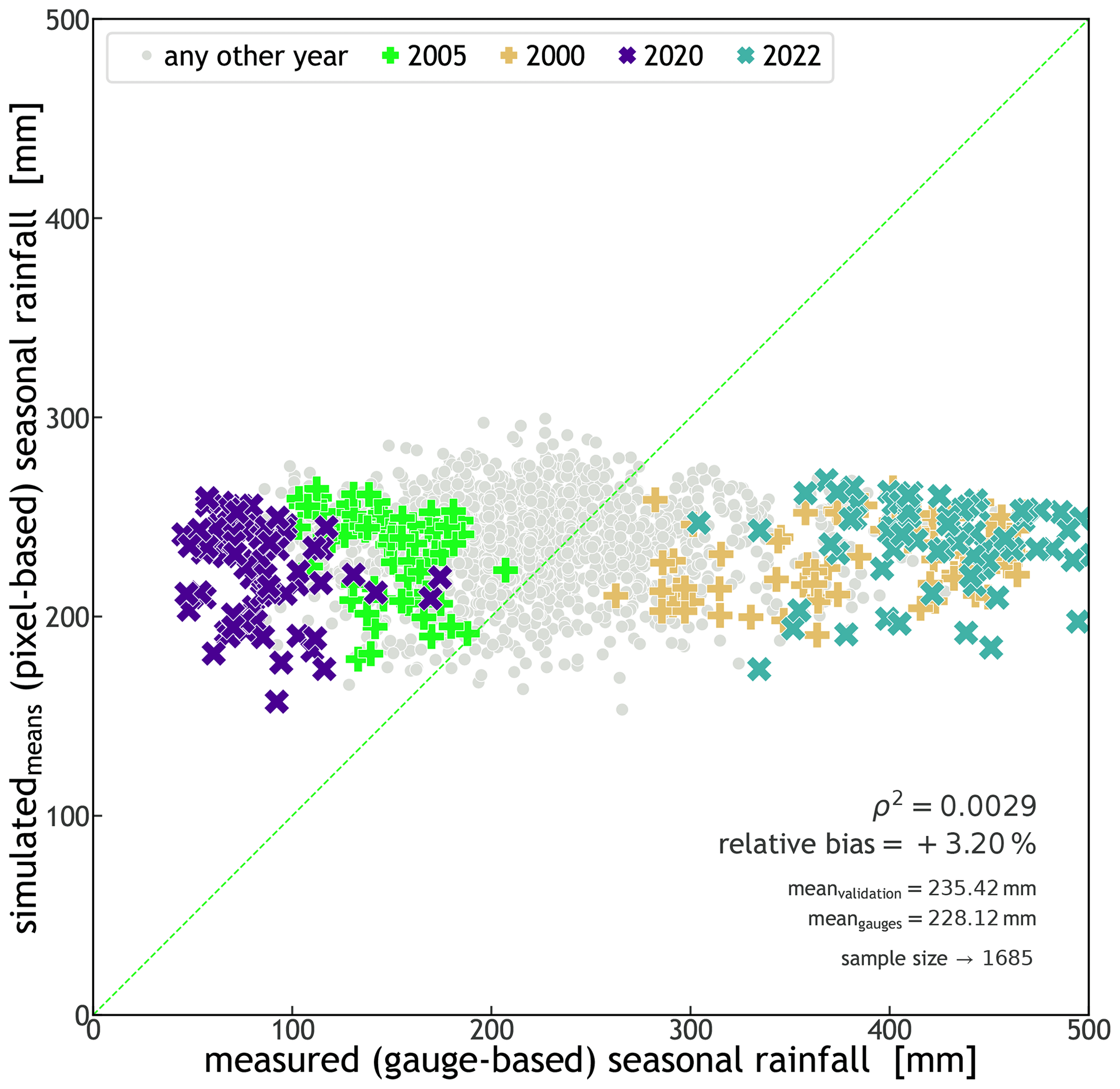
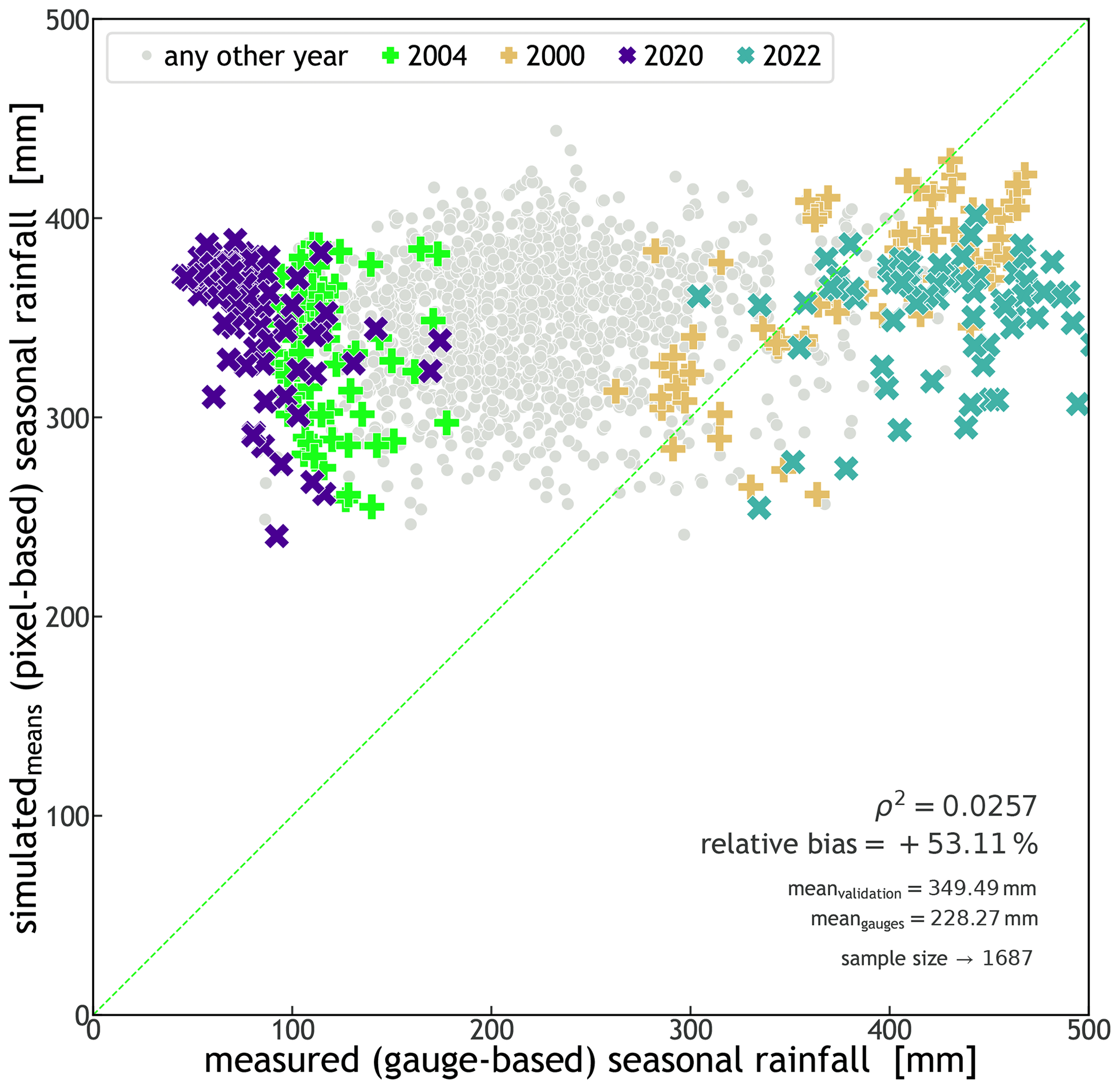
Figure 5 Scatter plot of simulated (means) seasonal rainfall against measured seasonal rainfall. Each marker represents a pixel/station for which the seasonal totals of 30 simulations were averaged (y axis) and the actual seasonal total recorded for that location (x axis). The × markers indicate the wettest (2022) and driest seasons (2020) from 2000 through 2022. Within the plot, the coefficient of determination (ρ², which is the square of the coefficient of correlation) is indicated. The medians of the datasets, the relative bias between them, and the size of the sample (an average of 73.3 gauges per year) are also shown. The green line indicates a 1:1 line. The very low coefficient of determination (ρ²=0.0028) indicates STORM's inability to explicitly simulate extreme rainfall seasons either wetter or drier than those present in the historical records.

The boxplots in Fig. 6a represent the distribution of the number of storms during the wet season for both validation (blue) and gauge (orange) datasets. Once again, one can see how STORM, despite being close to the average number of storms in a season (32), fails to account for the inter-annual variability in storm rainfall present in the gauge records. The average number of storms for the gauge data is (39). When disaggregated by year (see Fig. 6a), the maximum average number of storms (66.3) is found for the year 2022 (with a global maxima of 79 storms), whereas the minimum average (20.6) is for 2020 (13 storms for global minima). As illustrated in the scatter plot, 2022 and 2020 match the years for maximum and minimum (average) seasonal totals, respectively, indicating the direct relationship between the number of storms in a given season and its total precipitation.

We selected three gauges sparsely located throughout the WGEW and compared the temporal distribution of their median and mean storm intensities. The boxplots in Fig. 6b (all three rows) show that the median yearly storm intensities produced by STORM (blue boxes) are consistently lower than the median yearly intensities measured by the gauge network (orange boxes). On average, and throughout the whole validation exercise, the average median storm intensities from gauge data (4.0 mm h⁻¹) is 48.8 % larger than the average from the medians of simulated storms (2.7 mm h⁻¹). Nonetheless, and when accounting for the mean, recorded storm intensities (7.1 mm h⁻¹) are 16.2 % lower than the mean of simulated storm intensities (8.5 mm h⁻¹). This is mainly attributed to extremely large simulated storms (see Fig. B6a). In spite of its inability to model inter-annual storm variability, the stochasticity embedded in STORM allows plausible storm intensities larger and smaller than those (ever) recorded by the gauge network (see Fig. B6a, where the average maximum simulated intensities is 12.6 mm h⁻¹, with maxima over 100 mm h⁻¹; see Sect. 2.1).

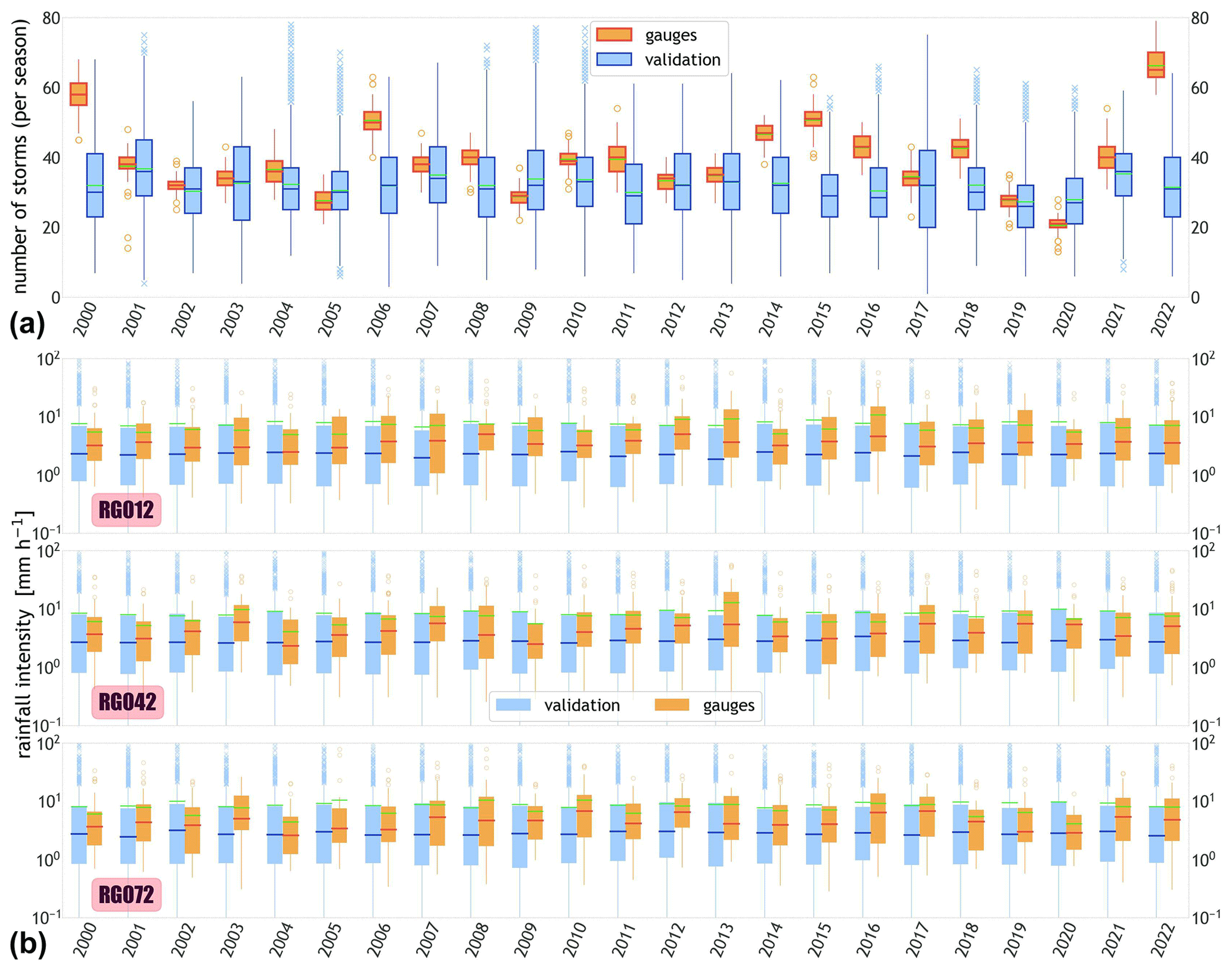
Figure 6 Yearly boxplots for the validation (blue) and gauge (orange) datasets. (a) Distribution of the number of storms in a wet season. (b) Distribution of storm intensities of three stations, i.e. RG012, RG042, and RG072, inside the WGEW. In both panels, the green line within each boxplot represents the mean of the distribution. Please note the logarithmic scale of the y axes in panel (b) (i.e. rainfall intensity). Figure B8 shows the (sparse) location of the aforementioned gauges.

One final validation exercise was to compare the top 10th percentile of all storm intensities of both gauge and validation datasets (simulated maximum intensities also included). The storms' maxima (by design; see Sect. 2.4) are found in the centres of the storms and can only be retrieved for the simulation dataset. The boxplots presented in Fig. B6b show that, despite STORM's ability to simulate (on average) extreme rainfall intensities about twice as large/high as those recorded by the gauge network, the top 10th percentile of maxima simulated intensities are 44 % larger than the top 10th percentile of storm intensities in the gauge set. Figure B6a shows that, on average, mean maxima intensities (12.6 mm h⁻¹) are 76.5 % larger than the mean of actual/recorded intensities (7.1 mm h⁻¹) and 47.9 % larger than average simulated intensities. The above suggests the robustness of the methodology here developed to account for maximum intensities when simulating the storms. It also incorporates the theoretical understanding that individual gauges are unlikely to have recorded the maximum storm intensities.

3.2 Testing climate drivers

To evaluate the ability of STORM to account for potential future climate change scenarios, we carried out two additional validation exercises: one where TOTALP is increased by a fixed scalar throughout the whole period, i.e. $\text{PTOT\_SC}=+\mathrm{0.5}$, representing a wetter climate, and the other where MAXINT is reduced by a progressive scalar, i.e. $\text{STORMINESS\_SF}=-\mathrm{0.035}$, representing a decline in storm intensity. We are aware that these two scalars might not be realistic or even at all plausible. Still, we chose those numbers as they enable drastic changes in the final outputs, thus allowing straightforward comparisons between these “climate change” results and the ones presented for the default validation (i.e. where no climate controls are simulated).

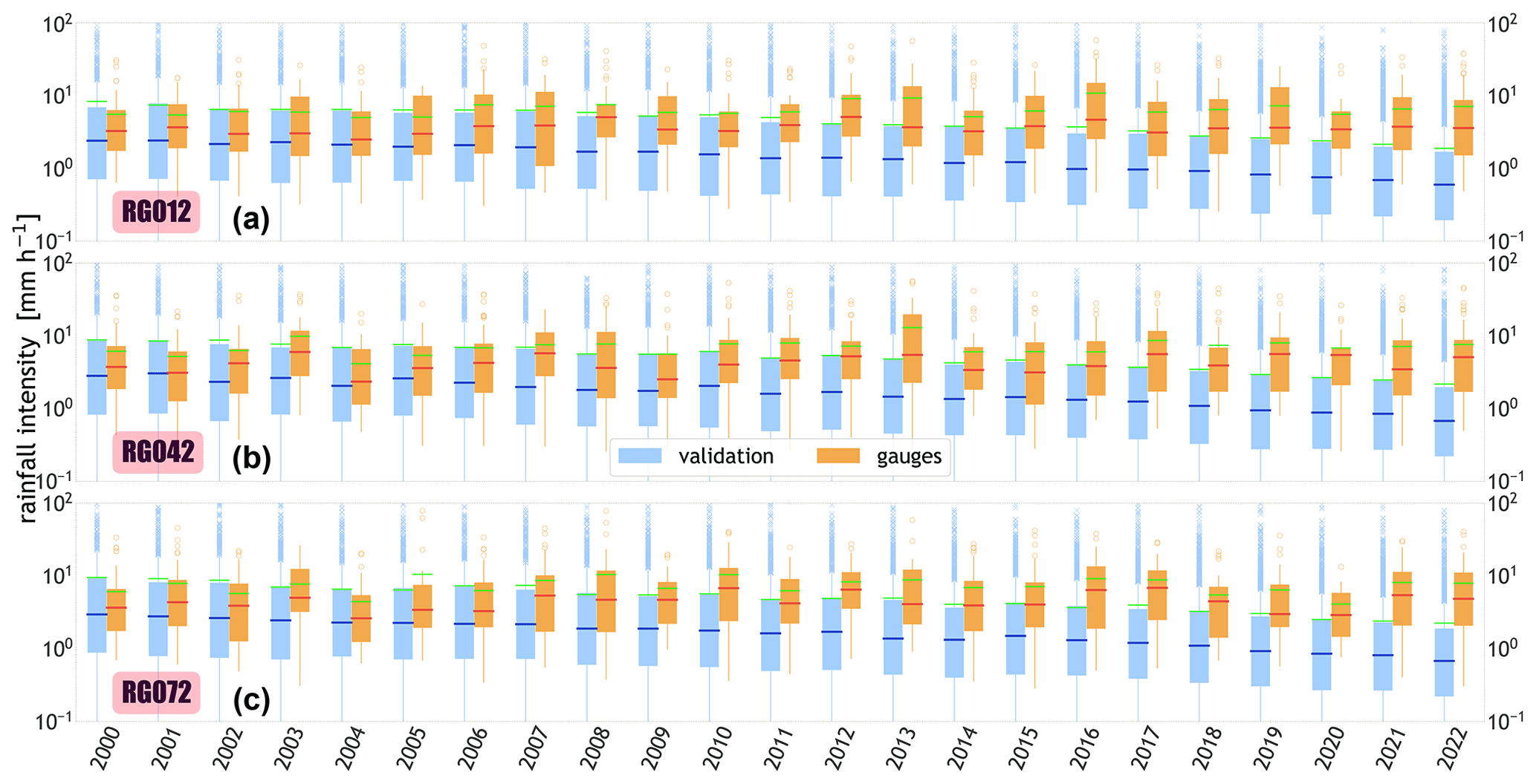
Figure 7 Yearly boxplots for the validation (blue) and gauge (orange) datasets. The boxplots represent the distribution of storm intensities of three stations, i.e. RG012, RG042, and RG072, inside the WGEW (respectively, top, middle, and bottom rows). In all rows, the green line within each boxplot represents the mean of the distribution. Please note the logarithmic scale of the y axis (i.e. rainfall intensity). Figure B8 shows the (sparse) location of the aforementioned gauges. This plot is equivalent to Fig. 6b, except that here we force the sampled maximum storm intensity (MAXINT) to be 3.5 % lower than the previous year. Thus, and after 23 years of simulation, the (mean) decrease in maximum storm intensity is 77 % (less).

With a progressive factor, $\text{\_SF}=-\mathrm{0.035}$, applied to the MAXINT variable, we force the sampled maximum storm intensity of every simulated year to be 3.5 % less than the year before. Hence, for a validation run of 23 years, one can expect that in the last simulated year the (mean) decrease in maximum storm intensity would be 77 % (i.e. $(\mathrm{23}-\mathrm{1})\times \mathrm{0.035}$) less than the first simulated year. The above can be seen in the yearly boxplots presented in Fig. 7. For any of the gauges presented in Fig. 7 (e.g. gauge RG042), one can see how the median rainfall intensity of the validation dataset, i.e. 0.68 mm h⁻¹ at the end of the simulated period (2022), is 76 % less than the median at the starting of the simulation (2000), i.e. 2.82 mm h⁻¹. The value is 86.7 % less when compared to the median at the end of the actual records (i.e. 5.08 mm h⁻¹). In STORM 1.0, the progressive factor SF (over the MAXINT variable) is referred to as the “temporal trend in storminess” (Singer et al., 2018).

With a constant factor, $\text{\_SC}=+\mathrm{0.5}$, applied to the TOTALP variable, we force the sampled seasonal total rainfall of every simulated year to be 50 % higher than it normally would. Hence, no matter what year of a given validation one is running, the expected (mean) increase in seasonal total will be roughly constant. This effect can be seen in the scatter plot presented in Fig. 8. In this figure, the cloud of points (scatter) has shifted upwards 48.5 % of the mean value for simulated seasonal totals presented in Fig. 5, corresponding to a validation were no climate change scaling factor was applied. In STORM 1.0, the constant factor SC (over the TOTALP variable) is referred as “step change in wetness”.

Figure B7 shows how the number of storms (in a wet season) is modified due to the (two) aforementioned climate change factors. For the case in which TOTALP is increased by a fixed scalar (i.e. Fig. 8), STORM generates (on average) more storms per season in order to reach the increased total seasonal rainfall. For the case in which MAXINT is progressively reduced by a progressive scalar (i.e. Fig. 7), STORM is forced to continually increase the number of storms in order to reach the median (sampled) seasonal total.

Figure 8 Scatter plot of simulated (means) seasonal rainfall against measured seasonal rainfall. This plot is equivalent to Fig. 5, except that here we force all simulated seasonal totals to be (every time) 50 % larger than the sampled total seasonal rainfall (TOTALP).

3.3 STORM applications

These improvements to STORM 1.0 now make STORM suitable as a climate driver of other watershed response models that simulate hydrology (surface runoff, infiltration, and streamflow) (Michaelides and Wilson, 2007; Michaelides and Wainwright, 2002), groundwater recharge during and after rainfall events (Quichimbo et al., 2021), interactions between streamflow and alluvial aquifers (Evans et al., 2018), or even for representing ecohydrological responses of vegetation to climate forcing (e.g. Warter et al., 2023). It also enables STORM to be useful in water balance models (e.g. land surface models) to assess water availability to plants through dynamic ecohydrological simulation of plant–climate interactions and water utilization (Warter et al., 2021; D'Odorico et al., 2007; Caylor et al., 2006; Laio et al., 2006), as well as energy/carbon fluxes between the land surface and the atmosphere (Best et al., 2011; Bonan, 1996). Finally, STORM can also be used to drive geomorphic models that characterize erosion and deposition processes within drainage basins in response to sequences of rainfall and runoff (Michaelides and Singer, 2014; Michaelides and Martin, 2012) and even landscape evolution models that simulate landform development over longer timescales (Hobley et al., 2017; Tucker and Hancock, 2010). Coupling STORM to such models would enable a wide range of scientists to investigate key problems in the environment that have their origin in the climate system. These problems range from which water sources are used by plants (Sabathier et al., 2021; Sargeant and Singer, 2016; Singer et al., 2014; Dawson and Ehleringer, 1991) and what is the dominant source and timing of groundwater recharge (Quichimbo et al., 2020; Cuthbert et al., 2016; Wheater et al., 2010; Scanlon et al., 2006) to the role of climate in shaping landscape morphology (Michaelides et al., 2018; Singer and Michaelides, 2014; Tucker and Bras, 2000; Tucker and Slingerland, 1997). The new STORM could also be integrated with stochastic models characterizing atmospheric evaporative demand (e.g. Asfaw et al., 2023), which would allow for closure of the water balance.

4 Summary and conclusions

Built upon STORM 1.0, STORM (https://github.com/feliperiosg/STORM2, last access: 7 July 2024) is an improved stochastic rainfall generator applicable to (small) gauged watersheds (with detailed rainstorm records) in any climatic zone. This stochastic framework heavily relies on PDFs of the total seasonal rainfall (TOTALP), maximum storm radius (RADIUS), decay rate of maximum rainfall from the storm's centre towards its maximum radius (BETPAR), maximum rainfall intensity (MAXINT), average storm duration (AVGDUR), copula's correlation parameter (COPULA), storm start date (DOYEAR), and (optional) storm start time (DATIME). The main modelling features of STORM with regard to its predecessor are storm intensity and duration represented via a (bi-variate) Gaussian copula framework, intensity–duration copulas at different elevation bands within the catchment, storm time occurrence via a circular statistics approach (i.e. mixture of von Mises PDF) or via discrete PMFs, storm start times via a circular statistics (optional), an alternative implementation of future climate scenarios, an output compressed into (georeferenced) NetCDF files and readily available for visualization, and a pre-processing module to construct all necessary PDFs from gauge data. Added to STORM, and with a future mindset of its applicability at larger scales, we implemented capabilities such as PDFs easily defined by the user (or retrieved from gauge data), storm simulation with regard to elevation (provided a digital elevation model – DEM), customizable spatial resolution (and coordinate reference system – CRS), spatial operations under a raster framework (thus adding speed, versatility, and scalability), and an optimal output storing in NetCDF format.

To develop the stochastic model, we derived and calibrated all PDFs to 37 years of storm data collected by an analogue network of 118 gauges sparsely deployed over the WGEW (148 km²). To test the performance of the model, we carried out one validation exercise consisting of 30 runs, with each one having 23 simulated years (i.e. 690 simulation years in total). The output of such a validation run was compared against 23 years of storm data collected by the digital network of 93 gauges located within the WGEW. To evaluate STORM's ability to model rainfall under potential future climate scenarios, we carried out two more validation runs, with each one comprising 690 simulation years too. These results were also compared against the digital/automatic gauge network.

Results showed that the seasonal total rainfall reached by STORM is 5.5 % lower than the actual records when accounted as the spatial median of all the stations/pixels within WGEW (see Fig. 4b). If accounted on a temporal basis, i.e. without any spatial averaging, then this relative difference amounts to +5 % (see Fig. 4a). On a seasonal basis, the storm mean rainfall intensity recorded by the gauge network is 16.2 % smaller than simulated storm intensities (see Fig. B6a). Nevertheless, the stochasticity embedded in our model allows for unrecorded but very plausible, either larger and/or smaller, storm intensities (see Figs. 6b and B6). Results obtained for the varying climate simulations showed that STORM is also able to imprint seasonal variability on rainfall (either in intensities or totals) in long-term analyses.

5 Constraints and recommendations

Future plans for the improvement of STORM will be focused on moving from drainage basins to regions, allowing for a wider range of applications such as land surface modelling. To achieve this, further improvements will be needed to characterize how rainstorm characteristics vary across a region so that they can be represented within STORM's PDFs. Finally, it will necessitate the use of gridded rainfall products for STORM to inform on the input PDFs.

The choice of a bi-variate Gaussian copula was mainly driven on its simplicity/easy configuration and applicability. Nevertheless, a further improvement (at least conceptually) might be the implementation of more elaborate copula models (and truly applicable to the intensity–duration case) like extreme values, Archimedean, etc. (e.g. Chen and Guo, 2019; Zhang and Singh, 2019; Salvadori and De Michele, 2006).

STORM's current weakness is its inability to account for other local hydrometeorological patterns and global teleconnections that may contribute to intra- and inter-seasonal rainfall variability (see Figs. 5 and 6a). This is something expected, as STORM (by design) does not incorporate any PDF that describes the behaviour of such inter-annual variability. Nevertheless, STORM's flexibility allows any user to roughly model the eventual impact of such teleconnections via the scaling factors PTOT_ or STORMINESS_ (see Sect. 2.8).

Appendix A: BIC estimation

The Bayesian information criterion (BIC; also known as Schwarz's Bayesian criterion – SBC) is a metric used for the unbiased assessment of the optimal number of M-unimodal vM distributions (e.g. Rios Gaona and Villarini, 2018; Lark et al., 2014). Such a criterion allows the selection of the least complex of all the models in consideration, i.e. the one with the lowest BIC. From a mathematical point of view (Eq. A1), BIC (or similar models, i.e. AIC – Akaike's information criterion) combines the maximized log likelihood of the fitted model with a penalization term that is related to the number of estimated parameters (Pewsey et al., 2013, Eq. 6.3).

$$\begin{array}{}\text{(A1)}& \text{BIC}=\mathit{\nu }\cdot \ln \left(n\right)-\mathrm{2}\cdot {\mathrm{\ell }}_{\max },\end{array}$$

where ℓ_max is the maximized (full) log-likelihood of a model with ν degrees of freedom and n the number of observations.

Figure A1 Bayesian information criterion (BIC) for mixtures that go from one to nine von Mises (vM) probability density functions (PDFs). The blue line is for the BIC of day of year (DOY), whereas the red line is for the BIC of time of day (TOD). The colour of the y axes indicates the values of their respective BICs. The black circles indicate one of the lowest points of the related BIC curve. The lower the BIC, the more optimal the number of vM PDFs (in the mixture) that best describes the sample multi-modality. Thus, to avoid the selection of a model with too many vM PDFs, the black circles also indicate where the change in slope is more drastic, even if they are not global minima.

Unfortunately, the vonMisesMixtures package does not offer a way to retrieve the maximized log-likelihood from which to compute the BIC of the mixture of M-unimodal vM PDFs. Unlike Python's vonMisesMixtures package, R (R Core Team, 2023), jointly with the movMF package (Hornik and Grün, 2014), does offer the possibility for an easy retrieval of BIC estimates for fitted MvM PDFs (Fig. A1). The implementation of such a feature in STORM was beyond the scope of this work. Nevertheless, STORM does offer the script pre_processing_circular.R from which the entire circular analyses (BIC included) can be computed. Once this analysis is carried out, the user will have all the necessary elements to discern the optimal fit for their “circular” data.

Figure A1 shows the DOY, and TOD BICs for mixtures ranging from one to nine vM PDFs. Strictly speaking, and for the DOY case, the lowest BIC found in the figure is for a mixture of nine vM, i.e. −318370.54. One can argue that a nine MvM model certainly over-fits the multi-modality of DOY (see Fig. 3a) without even mentioning its computationally intensive parameter estimation. Nevertheless, if one looks at the five MvM model (BIC equals to −317840.12), one can see that the improvement of the BIC metric is increasingly very small beyond this point in comparison to the one to four MvM models. Therefore, we are confident that a five MvM model not only accurately describes the multi-modality of DOY (for the WGEW dataset) but also is faster in its parameter estimation with regard to any larger (i.e. more vM PDFs) model. Hence, a mixture of five vM PDFs is the default configuration for DOY in STORM. Following that train of thought, we found the three MvM model the optimal mixture for TOD and thus its default settings in STORM.

Appendix B: Additional figures

Figure B1 Probability density functions (PDFs) for maximum storm extent (RADIUS; see Sect. 2.3). The cyan area represents the histogram of maxima radii estimated from three or more gauges, whereas the salmon area is for a maxima radii distribution (obtained) from two or more gauges. The solid blue line indicates the best fit for the cyan histogram, i.e. a Johnson's S_B PDF (see Table 4; row 2). The dashed red line is also a Johnson's S_B PDF (with parameters a=1.54, b=0.953, $\text{loc}=-\mathrm{0.228}$, and scale=18.289).

Figure B2 Probability density functions (PDFs) for storm rainfall measured by gauge data (salmon histogram) and for estimated maxima (cyan histogram). The solid blue line indicates the best fit for the cyan histogram, i.e. an exponential PDF (see Table 4; row 4), whereas the dashed red line (also a best fit) is a Pareto PDF. Maximum intensities are retrieved by fitting an exponential (quadratic) model $I\left(r\right)=I_{\max }\cdot e^{-\mathrm{2}\cdot {\mathit{\beta }}^{\mathrm{2}}\cdot r^{\mathrm{2}}}$ to measured storm rainfall (see Sect. 2.4). Note how the mean from estimated maximum intensities (μ=7.10) is larger than the mean of rainfall intensities measured by gauges (μ=4.98) prior to any model fitting.

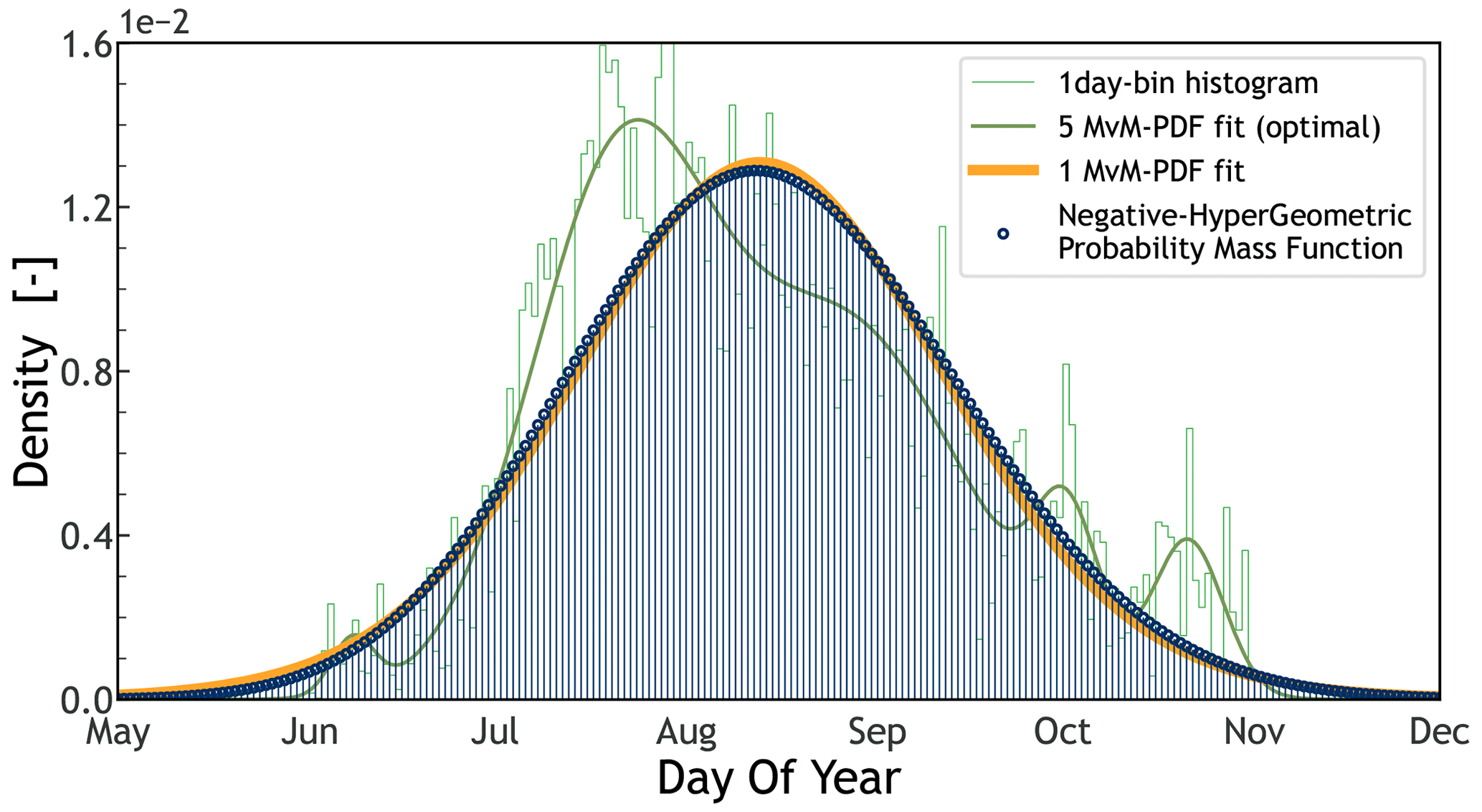
Figure B3 Probability mass function (PMF – vertical lines ending in blue circles) of a negative hyper-geometric family fitted (best fit) to a distribution of storm start day of year (DOY – green histogram). The coarser green line represents the optimal fit of a mixture of five von Mises (MvM) PDFs for the aforementioned distribution, as presented also in Fig. 3 (over a “circular” space; see Sect. 2.7). The orange line is a one MvM PDF. Note its similarity with the PMF and its poor fit of the underlaying DOY distribution with regard to the five MvM PDF fit.

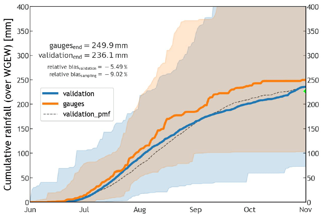
Figure B4 Percentile time series for the 100th percentile of all time series from June through October (wet season) for the simulation/validation (blue) and gauge (orange) datasets. The solid lines represent the median(s) of each dataset (50th percentile). The dashed black line represents the median for a validation where DOY was modelled through a discrete PMF (see Fig. B3). The green marker at the end of the time series indicates the median of the sampled (simulated) values of total seasonal rainfall (TOTALP). By design, STORM stops once the sampled seasonal total is reached or surpassed (the probability of reaching exactly the sampled value is extremely low). Hence, the actual (median) simulated seasonal total will always be greater than the sampled TOTALP.

Figure B5 Distribution of storm station/pixel-based intensities by elevation bands (i.e. orography). Blue is for the validation dataset, whereas orange is for gauge data. The green lines represent the mean of the distributions. Please note the logarithmic scale of the y axis. The x axis, from left to right, indicates three elevation bands for which analyses were carried out, i.e. up to 1350 m a.s.l., between 1350 and 1500 m.a.s.l., and above 1500 m a.s.l. Given the low gradient in relative orography within the WGEW, rainstorm variability with regard to orography is not a stark characteristic in this case.

Figure B6 Distribution of storm station/pixel-based intensities (a) for all data, i.e. 100th-percentile and (b) for the top 10th percentile of all storm intensities. Blue is for the validation dataset, whereas orange is for gauge data. The green lines represent the mean of the distributions. Please note the logarithmic scale of the y axes in both panels. The rightmost column is for the maxima intensities found in the storm centres (see Sect. 2.4). Such storm centre maxima are only retrieved for the validation dataset (no way to account for them in the gauge set).

Figure B7 Distribution of the number of storms in a wet season for the validation (blue) and gauge (orange) datasets. (a) Validation case for which MAXINT is reduced by a progressive scalar, i.e. $\text{STORMINESS\_SF}=-\mathrm{0.035}$ (see Fig. 7). (b) Validation case for which TOTALP is increased by a fixed scalar throughout the whole period, i.e. $\text{PTOT\_SC}=+\mathrm{0.5}$ (see Fig. 8). All y axes are consistent with Fig. 6a to allow (visually) equivalent comparisons. Note how, in panel (a), STORM generates more storms per season in order to reach the now increased total seasonal rainfall, whereas, in panel (b), the progressive decrease in storm intensity forces STORM to continually increase the number of storms in order to reach the median (sampled) seasonal total.

Figure B8 Digital gauge network for the WGEW (from 2000 through 2022). The three bold markers, i.e. gauges/stations RG012, RG042, and RG072, indicate the geolocation of the gauges referred to in Figs. 6 and 7. Even though the grid is presented in lat–long coordinates (i.e. CRS WGS-84), the actual projection (in both panels) is the 2D Cartesian coordinate system known as NAD83/UTM zone 12N (i.e. EPSG:26912).