Merged Observatory Data Files (MODFs): an integrated observational data product supporting process-oriented investigations and diagnostics

A large and ever-growing body of geophysical information is measured in campaigns and at specialized observatories as a part of scientific expeditions and experiments. These collections of observed data include many essential climate variables (as defined by the Global Climate Observing System) but are often distinguished by a wide range of additional non-routine measurements that are designed to not only document the state of the environment but also the drivers that contribute to that state. These field data are used not only to further understand environmental processes through observation-based studies but also to provide baseline data to test model performance and to codify understanding to improve predictive capabilities. To address the considerable barriers and difficulty in utilizing these diverse and complex data for observation–model research, the Merged Observatory Data File (MODF) concept has been developed. A MODF combines measurements from multiple instruments into a single file that complies with well-established data format and metadata practices and has been designed to parallel the development of corresponding Merged Model Data Files (MMDFs). Using the MODF and MMDF protocols will facilitate the evolution of model intercomparison projects into model intercomparison and improvement projects by putting observation and model data “on the same page” in a timely manner. The MODF concept was developed especially for weather forecast model studies in the Arctic. The surprisingly complex process of implementing MODFs in that context refined the concept itself. Thus, this article explains the concept of MODFs by providing details on the issues that were revealed and resolved during that first specific implementation. Detailed instructions are provided on how to make MODFs, and this article can be considered a MODF creation manual.

1 Introduction

The Merged Observatory Data File (MODF) concept is based on the simple principle of combining measurements made by multiple co-located instruments from research observatories and campaigns into a single file that complies with already established data stewardship standards. Here, “observatory” refers to a facility that measures an extensive inventory of collocated geophysical variables that have been chosen with the intention of investigating specific, usually interrelated, physical processes in order to answer hypothesis-driven science questions. In this context, an observatory could be a land site or a research vessel. While it is standard scientific operating procedure to co-locate research-grade instruments both continuously at observatories and episodically for field campaigns (often side by side with routine operational station instruments with long operational histories), there are generally no standard procedures for coordinated data management such as those that have been developed for operational data. Thus, the data from separate instruments can be scattered between separate files with different authors, formats, metadata, physical archive locations, and use restrictions.

The specific MODF realization presented here is for Arctic observatories (Uttal et al., 2016; Mariani et al., 2022) and field campaigns that resulted from initiatives established during the Year of Polar Prediction (YOPP; Goessling et al., 2016; Jung et al., 2016; Wilson et al., 2023). One key YOPP activity was the YOPP supersite Model Intercomparison Project (YOPPsiteMIP; Day et al., 2023), which was designed to facilitate the process-based validation of numerical weather prediction (NWP) models at polar locations during special observing periods (SOPs). The concept of MODFs and their forecasting analogs, Merged Model Data Files (MMDFs), was motivated by the YOPPsiteMIP community's desire to have the same variables from observations and models in easy-to-use files of the same structure in order to explore small-scale parameterized processes that are not represented well in the forecast models. These MODFs thus provide an integrated observation database to support model process representation through parameterization improvements for weather forecasts in the polar regions. At the same time, they also facilitate comparative observational studies across Arctic sites.

The MODF concept addresses the problem that research-grade, process-level observations are currently underutilized for model evaluation of parameterization deficiencies. As weather forecasting models increase in complexity and include detailed representations of land, the ocean, ice, and snow in addition to the atmosphere, it is increasingly important to evaluate processes using observations recorded throughout the whole earth system column, including the fluxes at their interfaces, to inform model development. This requires the use of multi-variate process-oriented diagnostic methods which utilize data that span these multiple components to understand model error. An essential component of the MODF concept is that analogous Merged Model Data Files (MMDFs) can be developed with extracted model data from locations near and around the observatory sites. Together, these are defined as Merged Data Files (MDFs). The MDFs, which bring together observations from different earth system components as well as model output in a standard file format, provide the basis for this and will support model intercomparison and improvement projects (MIIPs) as an evolution from model intercomparison projects (MIPs). The idea of MIIPs (a new acronym that we define here) does not imply that previous MIPs did not have productive results. However, through the development of matched MODF and MMDF data sets, it is implied that what have often been intercomparison studies can be smoothly extended to model improvements.

2 Background

Using observations and model outputs symbiotically is an area of ongoing effort and research with recognized challenges (Holtslag, et al., 2013). Many levels of MIPs have been in progress for decades (Stephens et al., 2023). In addition, existing efforts and methodologies facilitate the usage of increasingly heterogeneous data sets in model–observation fusion efforts through assimilation (Gettleman et al., 2022) and for inputs into multivariate artificial-intelligence analyses (Boukabara et al., 2021). There are well-organized systems for managing the data from operational surface networks, upper-air networks, and satellites that are uploaded into the Global Telecommunications System (GTS), which is overseen by the World Meteorological Organization (WMO) (see Global Telecommunications System (GTS), 2023; WMO, 2020). However, GTS data are only readily available directly to national forecasting centers (which presumably have developed institutionally specific reading and ingesting routines) and via products developed by WMO institutional repositories (https://climatedata-catalogue-wmo.org/, last access: 27 June 2024) (Bojinski et al., 2014; Lavergne et al., 2022). The latter have necessarily gone through various quality control, formatting, averaging, and (sometimes) interpolation steps to create globally uniform products. As a result of the standardized processing, it is likely that information on high-resolution, rapid, and extreme events (Sardeshmukh et al., 2015) may have sometimes been lost.

The MODF schema has been specifically developed for managing observatory and campaign research observations as opposed to operational observations. Research observations target local-scale and often rapid or extreme processes that are intended to lead to the discovery of the physics within the atmosphere as well as the physics that governs the coupling processes between the atmosphere and the underlying surface. The surface can be land, ocean, ice, or any of the three, often with obfuscating layers of plant and/or snow cover that are themselves components of the system and separate objects of study. Research-grade data pose many additional challenges regarding data latency, accessibility and uptake issues, and institutional ownership compared to data that have been managed more systematically specifically for operational purposes.

The data science community is aware of these issues and, in response, has developed FAIR (findable, accessible, interoperable, reusable) data principles (Wilkinson et al., 2016) that can be applied to individual data sets. However, Wilkinson et al. (2016) explicitly stated that “These high-level FAIR Guiding Principles precede implementation choices, and do not suggest any specific technology, standard, or implementation–solution; moreover, the principles are not, themselves, a standard or a specification.” Whereas many FAIR solutions are implemented by web services (e.g., Buck et al., 2019), the MODF concept described here can be considered an alternative: an integrated data product that is based on the same metadata conventions that have been developed for web service solutions. The considerations and steps described here for creating MODFs can therefore be considered a particular FAIR implementation–solution specifically for observatory and campaign data.

3 The MODF concept

Figure 1 is a conceptual schematic of the end-to-end process involving data collection, data quality control (QC) and processing, metadata information collection, and data amalgamation into netCDF files (Unidata, 2023) that follow the NetCDF Climate and Forecast (CF) metadata conventions (Eaton et al., 2022, hereafter the “CF conventions”). The process for turning model forecast output into MMDFs is qualitatively similar,¹ including the use of a particular set of global and variable attributes, since the specifications were developed by modelers as well as observationalists.

Figure 1 Instruments, measurements, data processing, and metadata generation for (a1) the atmospheric state at the surface, (a2) broadband radiation at the surface, (a3) surface turbulent fluxes, (a4) upper-atmospheric profiles, (a5) the terrestrial subsurface, and (a6) ocean and sea ice/snow. This information is collected into netCDF files with specified (b) global attributes and (c) variable attributes that are compliant with FAIR principles.

The different types of geophysical data (A1 through A6) that can typically comprise observatory and campaign research data are described below.

3.1 Surface atmospheric measurements

Surface atmospheric measurements at observatories or during campaigns are made with research-grade thermometers, hygrometers, and anemometers, with measurements often performed at a higher frequency and with more carefully calibrated sensors compared to operational weather stations. Such observations are sometimes performed side by side with operational weather service station measurements, providing context to multi-decadal operational records. Research meteorological measurements are frequently redundant; they are performed at multiple locations across a site (on a scale smaller than an NWP model grid cell) or at different levels on towers to get detailed profiles for the near-surface boundary layer. The variables measured are the temperature, pressure, relative humidity, and eastward and northward components of the wind speed. Both operational and research measurements of these atmospheric state variables can be considered to have well-quantified uncertainties determined by the instrument calibration and tolerances.

Broadband surface radiation is measured by radiometers that measure both incoming and outgoing shortwave and longwave radiation. There are multiple commercial and experimental instrument options for measuring broadband radiation, and in the Arctic, a particularly wide range of methods must be applied to keep glass domes clear of obstructions (e.g., ice, snow, dust, or sea salt), such as heating, ventilation, and manual cleaning (Cox et al., 2021). The Baseline Surface Radiation Network (BSRN) (Ohmura et al., 1998) is a global repository for standardized radiation products that are traceable to the WMO World Radiation Radiometric Reference. However, the BSRN is not designed to accommodate short-term campaign data sets and does not account for different methods for data QC and processing (Matsui et al., 2012; Long and Shi, 2006, 2008).

Surface turbulent flux variables are calculated and inferred by a number of different methods. Eddy-correlation techniques (Kaimal and Finnigan, 1994) are based on measurements by fast-response sonic anemometers and hygrometers with built-in fast-response temperature sensors. It is often necessary to make considerable site-specific adjustments to processing methods, accounting for the local surface roughness, sensor height, and obstructed wind-direction sectors. In the polar regions, sensors operate near the thresholds of instrument ratings for detection and environmental conditions and have to be quality checked for periods of riming. There are specific challenges relating to the cold snow-and-ice-covered surface conditions over land (Grachev et al., 2018) and over the ice pack of the central Arctic Ocean (Andreas et al., 2010; Cox et al., 2023). Eddy-correlation methods are only valid under stringent environmental conditions, which results in frequent data gaps. Alternatively, turbulence variables can be calculated by bulk-aerodynamic methods (Monin and Obukhov, 1954; Mahrt and Sun, 1995), but results are not as meaningful when comparing to models as this becomes a model-to-model rather than a model-to-observation comparison. Commercial packages for calculating latent, sensible, and gas fluxes have been developed and compared (Mauder et al., 2008; Fratini and Mauder, 2014), but caution must be exercised when using the results, and it is important to understand the basis on which variables are derived by proprietary commercial or custom software. The resulting flux variables are the latent and sensible heat fluxes, friction velocity, surface stress (momentum flux), drag coefficient, kinematic temperature scale, Monin–Obukhov stability parameter, and dissipation rate of the turbulent kinetic energy. Given the variety of physical conditions and complex methodologies for calculating turbulent fluxes, an assessment of the interoperability and consistency between flux products from different data collections is still necessary, despite the existence of operational flux data networks such as FLUXNET (Baldocchi et al., 2001) and AmeriFlux (Baldocchi et al., 1996; Boden et al., 2013).

Solid and liquid precipitation are both measured at the surface but are notoriously difficult to characterize accurately. Precipitation accumulation is traditionally measured at frequencies ranging from every hour to every 6 h by gauges within a surface precipitation network that is usually operated by operational weather centers or hydrological agencies. Measuring solid precipitation presents a number of unique challenges; snow pillows and the double-fence automated reference (DFAR) configuration around gauges provide reliable estimations of precipitating snow. However, snow precipitation measurements from WMO standard installations with single-Alter-shielded and unshielded gauges are affected by an undercatch of solid precipitation in windy conditions (Nitu et al., 2018; Kochendorfer et al., 2022). The WMO Solid Precipitation Intercomparison Experiment (SPICE) analyzed this undercatch and developed adjustment functions for correcting it (Kochendorfer et al., 2018; Wolff et al., 2015), which are now being used in verification practices (Køltzow et al., 2020; Buisán et al., 2020; Casati et al., 2023).

3.2 Upper-atmospheric profiles

Radiosonde data are typically treated as if they are instantaneous vertical profiles of the troposphere by collapsing the balloon-borne trajectory of the instrument package into a profile that is time indexed with the launch time. The measurements of temperature, dew-point temperature, pressure, humidity, and winds are high cadence (on the order of seconds) during the balloon ascent, with individual launches being low cadence (every 12 h, with standard launch intervals at 00:00 and 12:00 UTC). During intensive campaign periods, the launch frequency is often increased to 4–6 sondes per day. A full sounding can take 2 h to ascend and can travel up to 200 km horizontally, and important fine-scale information is available if the full original trajectory information (time–height/pressure level–latitude–longitude) coordinates are maintained to assess the spatial displacement. Sometimes, special arrangements are made to continue to capture data from the radiosonde during its descent after the balloon bursts (Hartten et al., 2018), although care is necessary when using descent data because key assumptions built into the instrument design are being violated. For example, the temperature and humidity sensors are positioned on the sonde such that they sample air undisturbed by the instrument casing during ascent, but those conditions may or may not be met during descent (Ingleby et al., 2022).

Many observatories and campaigns support the operation of radars, lidars, sodars, profilers, and microwave radiometers which, separately and in combination, can remotely infer properties throughout the depth of the planetary boundary layer (PBL) and free atmosphere. The systems use active (transmission and the interpretation of the reflected signal) and passive (detection of the natural atmospheric signal) sensing techniques. Using a significant body of research on retrieval methods, the systems can determine properties such as the cloud base, cloud liquid-water path, cloud ice-water path, cloud liquid-water content, cloud ice-water content, hydrometeor sizes and shapes, snowfall rates (Matrosov et al., 2022), degree of riming, aerosol extinction coefficients, winds, temperature, and humidity. These advanced products may be obtained from diverse instrument hardware configurations and technologies as well as site-specific scanning and collection schedules. Robust site-independent retrieval methodologies that are consistent across networks – such as the products produced by Cloudnet (Illingworth et al., 2007) and the ARM Active Remote Sensing of Clouds product (Clothiaux et al., 2001) – have been developed; however, they may not be consistently implemented.

3.3 The terrestrial surface and subsurface

The terrestrial surface and subsurface are composed of different and complex soil, rock, ice (permafrost), and vegetation layers that can be covered with surface snow and ice that show evolving density, heat capacity, conductivity, and chemistry. Thermistor strings can be co-located with tensiometers; the variables measured are the gradients of temperature and moisture, respectively, with thermal conductivity and heat capacity determined as fixed intrinsic properties from soil samples. Thermistor strings can also be co-located with moisture probes, providing vertical profiles of soil temperature and moisture, respectively, down to depths ranging from 0.1 to 2 m, depending on the soil type. Snow depth, like precipitation, is a difficult quantity to measure representatively; techniques vary from using simple measurement stakes to downward-looking mast- or tower-mounted acoustic devices.

3.4 The ocean, sea ice, and the snow surface and subsurface

Ocean thermistor measurements are accompanied by conductivity and pressure measurements, which allow the determination of the salinity, temperature, and depth. Additional current meters allow the determination of turbulent fluxes using eddy correlation techniques similar in principle to those used for atmospheric fluxes. The measurement of sea-ice and snow macro- and microphysical properties below the atmosphere–ice or atmosphere–snow interface (i.e., the subsurface) is increasingly sophisticated, with upward- and downward-looking acoustic devices on ice buoys determining the ice thickness and snow depth (Zuo et al., 2018). Measurements are made of the snow and ice density, crystalline structure, and salinity via manual sampling.

4 MODFs for the Year of Polar Prediction

The WMO Polar Prediction Project (PPP) organized the Year of Polar Prediction (YOPP; PPP Steering Group et al., 2019; Jung et al., 2016), which concluded in 2022 (Wilson et al., 2023). The YOPPsiteMIP (Svensson et al., 2020; Day et al., 2023) working group envisioned matched sets of observation and model data to support model process diagnostics. The efforts of this working group resulted in a metadata schema for MODFs and MMDFs (collectively known as MDFs) as well as an iterative production workflow. The YOPPsiteMIP effort focused on polar terrestrial stations, but because it was anticipated that a similar strategy would be applied to the YOPP-endorsed Multidisciplinary drifting Observatory for the Study of Arctic Climate (MOSAiC) expedition (Shupe et al., 2022; Nicolaus et al., 2022), the schema was developed to also accommodate expected additional ocean and sea-ice observations from ships and on-ice platforms in the central Arctic Ocean.

The first steps in MODF production are to assemble the available data files that will feed into the MODF, extract the desired data, and acquire the corresponding metadata. During these steps, each individual instrument and instrument group requires both unique quality control and processing, together with attribution tracking, in order to produce the geophysical variables and to document their provenance. Given the heterogeneity and often research-grade nature of campaign data, the amount and quality of metadata for different variables is likely to be inconsistent. Although required metadata are ideally harvested from the internally documented data files, it is likely that many data sets will need additional metadata that will require interviewing the original data collectors (for an example of this other than our own, see Papoutsoglou et al., 2023). Once individual data and any available metadata from individual instruments and instrument suites are created and/or assembled, the merging process can begin.

As we developed the schema and workflow, we identified the following challenges and solutions.

Semantics. Data semantics address the issue of the same variable being given different names drawn from multiple or ad hoc naming conventions. A significant part of the MODF solution has been the development of an extensive schema based on already existing vocabulary standards.

Units. Variables' units are frequently absent entirely from data sets or expressed with nonstandard abbreviations (Hanisch et al., 2022). The MODF solution is to associate each variable with recommended units, typically as identified in the CF standard name table (2023). Eaton et al. (2022) explain how these are meant to be compatible with and generally recognized by the Unidata (2020) UDUNITS package.

Attribution. Perhaps the greatest MODF challenge is not technical but rather cultural. When data for a single MODF product come from instruments operated by multiple institutions and researchers, there are complex issues with acknowledging the original sources of the data (Pierce et al., 2019; Nature Editorial, 2022). Data from campaigns or programs usually have multiple institutions and individual researchers involved, all of whom have different performance metrics for original research. This often leads to official or implicit data embargoes so that the researchers who collected the data will have the first opportunity to publish research results. The design of MODFs is responsive to these issues as it provides a high level of attribution metadata, including links to original data and data producers, thereby supporting copious data citations (Vannan et al., 2020).

Data heterogeneity. Measurement heterogeneity is generated by differences in how data are collected and processed. The MODF solution is to, as much as possible, document variable derivation from the original data metadata: type of instrument, calibration information, method of deployment, quality control and processing histories, and original licenses.

Inconsistent cadences. Different variables are collected over a range of native cadences varying from Hz for the fast-response sensors needed to record phenomena that can change on short timescales (typically in the atmosphere) to sensors for which it is sufficient to sample on an hourly or even daily timescale (typically in the terrestrial subsurface), along with a wide range in-between (typically for the ocean and ice sub-surfaces). The MODF solution is for each variable to retain its native recording cadence and to minimize any temporal averaging beyond that necessary for sensible data processing. In addition, original data sets are not interpolated to fill data gaps.

Redundancy. It is common during campaigns or at intensive observatory sites for there to be multiple measurements of the same variable (e.g., temperature). There is important information contained in redundant measurements when evaluating how representative a variable is of site characteristics or when comparing in situ observations to model grid cells and satellite footprints to evaluate local variability. The MODF solution is to include as many redundant measurements as possible, maintaining high-accuracy location information that helps define the observations' microclimates, including, for example, soil and vegetation characteristics.

Processing levels. Research-grade data sets typically require unique quality control and often extensive post-processing, which can only rarely be fully automated. Frequently, the state variables (e.g., temperature) are readily available in near real time, whereas more complex variables such as turbulent fluxes can have a wide range of availability, depending on whether they are output by commercial software (Fratini and Mauder, 2014), calculated from bulk variables, or based on customized calculations for complex environments. The MODF solution is to include full processing, data-quality, and usability metadata.

Versions. Since it is common for observed data to have versions, the MODF concept accommodates multiple product releases. Examples of data versions include the raw data (sometimes just voltages); data that have been minimally quality checked by the automated elimination of extreme physically unrealistic outliers; data that have been subjectively curated for unusual and, if possible, correctable operational or environmental conditions; and data that have undergone different levels of processing to produce the retrieved variables (those based on more direct measurements). Frequently, highly processed and certified data are available months or even years after the original collection period. In some cases, all processing levels of data are available and archived. Two obvious ways of handling the situation are to either replace the original data with more processed data as they become available (Fig. 2a) or to keep all versions of the data (Fig. 2b). MODFs' rich metadata include careful version tracking for individual variables, which encourages the latter.

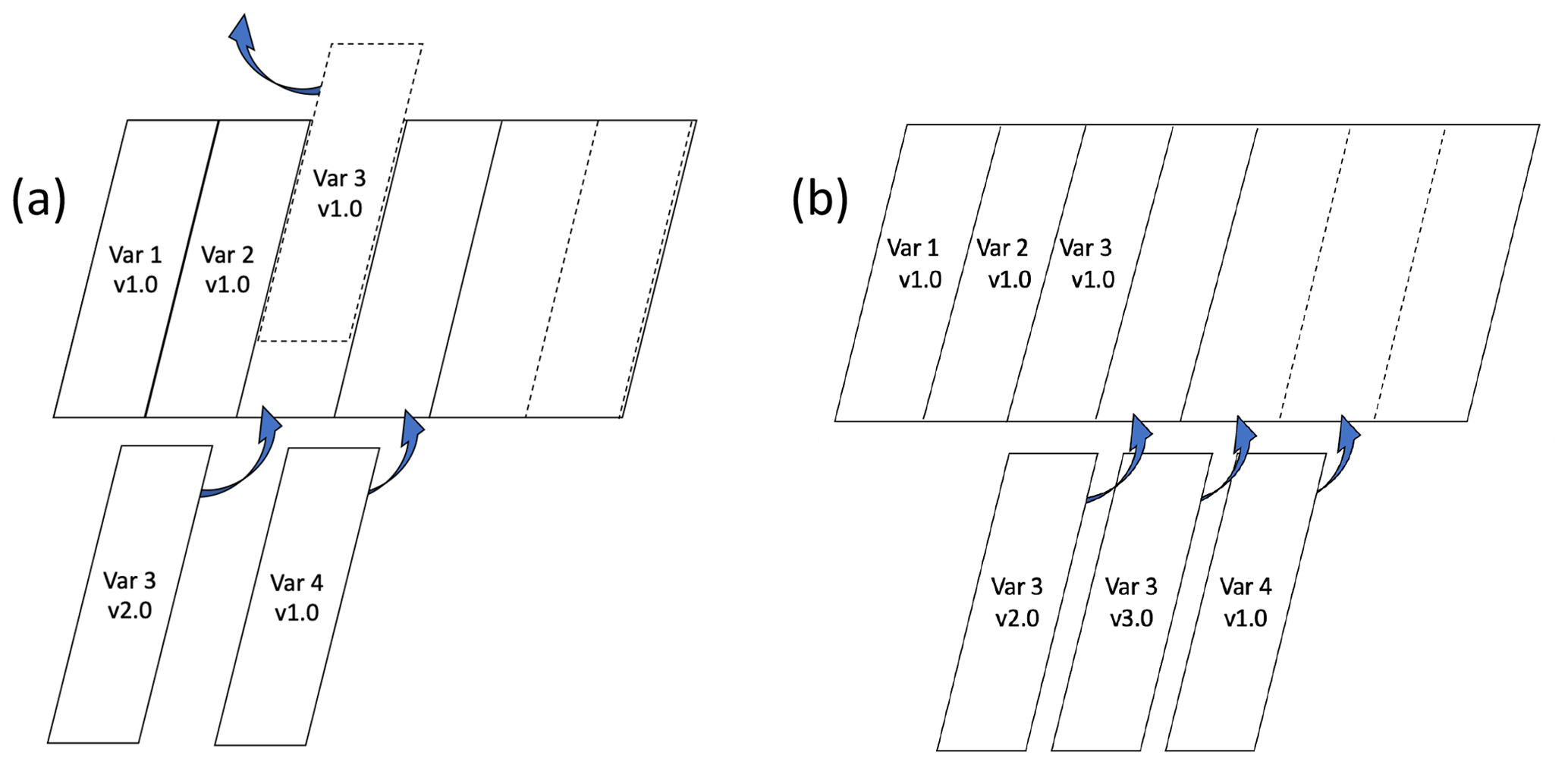
Figure 2 There are two approaches for MODF augmentation (as new variables become available) and modification (as variables proceed through processing levels). In both approaches, variables that are immediately available (Var 1, Var 2) can be immediately ingested and variables can be added as they become available (Var 3, Var 4). The two approaches accommodate two strategies for variables that undergo post-processing, which results in products with quality-control (QC) levels. In (a), the original data (Var 3 v1.0) can be replaced with quality-controlled data (Var 3 v2.0). In (b), the original data (Var3 v1.0) can be retained in the MODF, and quality-controlled data (Var 3, 2.0) can be added.

5 The H-K variable schema table

The H-K variable schema table, developed for the YOPPsiteMIP (Hartten and Khalsa, 2022; hereafter the “H-K schema”), provides guidelines for creating both MODF and MMDFs as netCDF files (Unidata, 2023) with consistent variable names and metadata. Hereafter, the discussion in this paper centers on those entries which are relevant to MODFs, although most of them are also relevant to MMDFs. The H-K schema follows the Attribute Convention for Data Discovery (2024; hereafter “ACDD”), the NetCDF Climate and Forecast (CF) metadata conventions (Eaton et al., 2022), and the ISO/TC 211 19100 series of standards for digital geographic information. Short variable names are compliant with the World Climate Research Program (WCRP) Coupled Model Intercomparison Project, Phase 6 (CMIP6; Taylor et al., 2022) whenever possible, as these are in wide use in the geophysical research community.

For global attributes, the H-K schema requirements include identifying the file feature type, the file maker, the license, the location, information on when the data were collected, and a permanent identifier. The global attributes listed in the H-K table are minimum requirements and may be augmented by others from the ACDD or the CF conventions in order to include other metadata deemed important for provenance or usability. In particular, the product_version global attribute can be used to help clearly identify when a MODF has been augmented by new or reprocessed variables, and comment can always be used for free-text metadata or stable URLs linked to additional metadata files. For variable attributes, the H-K schema identifies vocabularies, units, individual variable attributions (i.e., who originally collected the data) and variable provenance, and it also presents a method for the differentiation of multiple measurements of the same geophysical variable (redundancy). The H-K schema is available in both the JSON (machine readable) and PDF (human readable) formats.

5.1 Global attributes

Global attributes are the descriptive metadata that are relevant for the entire MODF file. Table 1 lists recommended global attributes for MODFs. Some were chosen because they are highly recommended by ACDD. Others are merely recommended by ACDD, but they made sense for our purpose and seemed not overly burdensome for those most likely to be making MODFs. We chose additional attributes from metadata standards other than ACDD – e.g., the CF conventions and the DataCite Metadata Kernel v4.4 (DataCite Metadata Working Group, 2021) – because we felt they would help MODFs be FAIR. Some global attributes whose inclusion and consistent use are particularly important are described below. We use italics for the names of attributes and single quotes around variable names.

id. The global unique persistent identifier (PID). This global attribute does not supersede references to the PIDs associated with individual variables (Prakash et al., 2016), which can be provided within the variable attribute references. The MODF id remains constant as modifications or additions are made to the MODF file.

license. Specifies the terms of distribution. As with id, individual variables and groups of variables in the MODF may have unique license requirements that can be recorded in the variable attribute comment.

creator_name. The names of individuals who should be in the citation for the MODF (Jones et al., 2020; see Sect. 2.2.7.3.3). The DataCite Metadata Kernel v4.4 (DataCite Metadata Working Group, 2021) defines creators in this context as the main producers of the MODF file and also links them to authorship. (Note that the main producers of component data sets are credited within the variable attributes that come from their individual data sets.) Enabling those who create MODFs to receive appropriate credit for their work is a key element of making MODFs FAIR; data reuse depends in part on data accessibility, which, in turn, is more likely when data are “considered legitimate, citable products of research” (Data Citation Synthesis Group, 2014).

featureType. Although the original vision was that each site during a campaign would have a single MODF that would include all relevant variables, when considering the practicalities of archive submission, it became apparent that the file featureType needed to be specified to facilitate data services such as visualization tools. Most observatory data fit into the featureTypes timeSeries, timeSeriesProfile, and timeSeriesTrajectory. These featureTypes are defined by the temporal–spatial dimensions that are associated with individual variables: time only for timeSeries, time and height (or depth) for timeSeriesProfile, and time–height (or depth)–latitude–longitude for timeSeriesTrajectory.

missing_value. Establishes one consistent missing_value for all data in the MODF.

history. Provides an audit trail for the MODF file, documenting its provenance. Initially, this should include information about how it was created. Later, if the original file is modified (e.g., variables are corrected or added), information about what has changed should be added to the original information. The CF conventions recommend that each step be documented by a line containing a datestamp, the name of the person or entity who did the action, a brief description of the action, and any program(s) which accomplished the action (including relevant settings or command arguments). If the modifications involve the addition of a new version of an existing variable, the variable attributes associated with the new version, and the earlier version if it is not removed, should thoroughly document the change.

Table 1 Recommended global attributes for the H-K schema (adapted from Hartten and Khalsa, 2022).

5.2 Time, space, and site variables

In the H-K schema, variables have been divided into subgroups. There are three subcategories with time, space, and site information: temporal dimensions and variables; spatial dimensions and variables; and single-level fixed variables. Per the NetCDF user's guide (Unidata, 2023), dimensions “may be used to represent a real physical dimension, for example, time, latitude, longitude, or height … [or] to index other quantities, for example station or model-run-number.” Examples of these indexing variables are listed in Table 2 and discussed further below. Per the H-K schema, all dimensional and geophysical variables are given a short CMIP or CMIP-like variable name and are characterized by variable attributes long_name, standard_name, units, additional recommended attributes, and any other attributes the MODF creators feel are necessary to fully document the data.

Table 2 Examples of dimensions and variables related to time, space, and site information, together with the associated long_name, standard_name, units, and recommended attributes (extracted from Hartten and Khalsa, 2022).

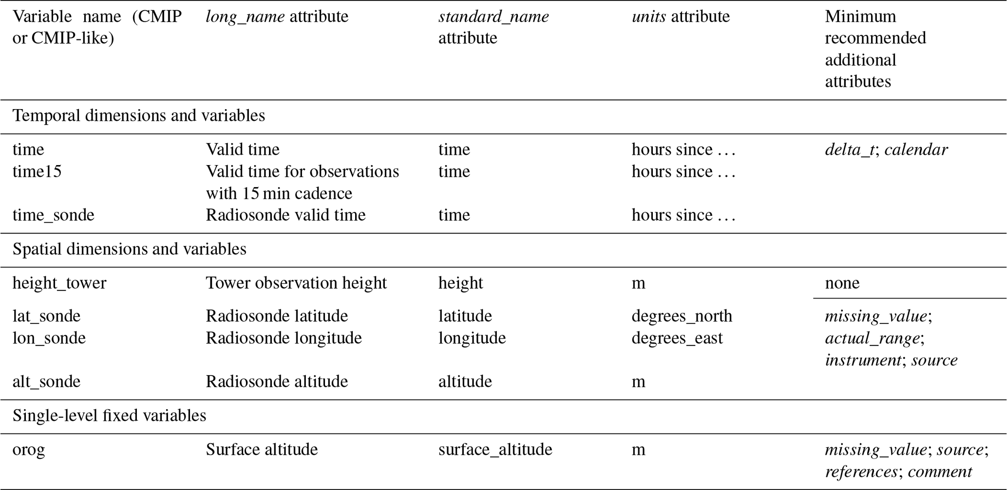
“time”; “time15”; “time_sonde”. MODFs are intended to retain as much high-resolution information from the original data collection as possible. Averaging is limited to that necessary for processing (e.g., for eddy-correlation flux calculations), and data are not interpolated. Therefore, temporal dimensions support maintaining the original data collection cadences for individual variables. For instance, in MODFs, “time” is a generic temporal dimension, whereas “time15” is a time dimension associated with variables collected at 15 min intervals and “time_sonde” is the time dimension associated with the data collected during a radiosonde ascent. In the YOPPsiteMIP implementation of MODFs, we have chosen to append “N” or “_platform” to a generic CMIP name such as “time” in order to indicate a time array with a particular cadence in minutes or a time array tied to a particular instrument or platform. In keeping with CF metadata guidelines, all the differently named time variables can and should have the same long_name attribute.

“height_tower”. A spatial coordinate can be a single scalar value or a set of values (a dimension) that describes the location where geophysical measurements are collected. This can be an array of fixed values in the case where measurements are made at set levels, for instance, on an instrumented tower. A tower may also consist of multiple measurements of the same geophysical variable collected at different heights above the ground. For instance, observations of air temperature collected by three sensors located at the surface (2 m a.g.l.), on a pole (10 m a.g.l.), and on top of a building (20 m a.g.l.) could be combined into a single array designated as “_tower” so long as the sensors' horizontal positions were co-located.

“lat_sonde”; “lon_sonde”; “alt_sonde”. Spatial coordinates can also be a dimension variable. For instance, if information on the latitude, longitude, and/or altitude of a radiosonde during its ascent is retained, this information should be put into auxiliary coordinate variables that provide the location in space for the geophysical variables collected by the sonde. If the sonde output includes only varying altitudes and a fixed launch time, the geophysical data from each sonde flight should be put into a file with the featureType “profile”. If the sonde output includes varying altitudes and associated times, the geophysical data should be put into a file with the featureType “timeSeriesProfile”. In both cases, a scalar altitude variable should be used as the vertical dimension for each flight. However, if varying values of the latitude and longitude are also provided, the geophysical data from each sonde should be put into a file with the featureType “timeSeriesTrajectory”, with the reported altitude, latitude, and longitude being provided as coordinate variables for each flight. Finally, the “profile”, “timeSeriesProfile”, and “timeSeriesTrajectory” featureTypes all require that times monotonically increase. It would be tempting (and not against the requirements of featureType) to put geophysical data collected during the radiosonde descent and their accompanying spatial coordinates into the same variables used for the values collected during radiosonde ascent. However, we would recommend using a separate set of variables with a clearly different suffix and long_ name set instead. Data collected during descent have different statistical characteristics than data collected during ascent (Stephan et al., 2021; Ingleby et al., 2022), and we think users should affirmatively choose, rather than accidentally use, such “off-label” data.

“orog”. Certain fixed variables describe the site or the platform from which measurements are taken. An example of the former is the variable with the surface altitude (CMIP name: “orog”), which describes the site's altitude above the surface defined as the lower boundary of the atmosphere. Other common single-level fixed variables are “lat” (latitude) and “lon” (longitude), which identify a site's general location. If the site has distributed measurements, individual variables may have more refined “lat_platform” and “lon_platform” variables or dimensions.

5.3 Geophysical variable attributes and examples

There are six categories of geophysical variables: single-level atmosphere variables; surface and top-of-atmosphere (TOA²) variables; atmospheric variables on model or instrument levels; subsurface terrestrial variables; oceanic variables on model or instrument levels; and sea ice variables. Examples of long_name, standard_name, and units attributes for observed geophysical variables that have been cataloged in the H-K schema are shown in Tables 3 and 4. A full listing of all the single-level atmospheric variables, the surface and TOA variables, and the atmospheric variables on instrument levels in the H-K schema version 1.2 is presented in Table A1, while a listing of the current H-K schema oceanic variables on model or instrument levels, subsurface terrestrial variables, oceanic single-level variables, and sea ice variables is found in Table A2. Some discussion of the examples in Tables 3 and 4 follows.

CMIP name. The Coupled Model Intercomparison Project (CMIP) names are taken from the CMIP6 Participation Guidance for Modelers, a program supported by the NASA Program for Climate Model Diagnosis and Intercomparison. CMIP names prioritize terse, presumably code-efficient abbreviations such as “ta” (air temperature). To clearly identify the variables that were observed or derived redundantly from different methods or platforms, a suffix can be appended (e.g., _tower, _radar, _8m). Some standard measurements, such as 2 m temperature and 10 m winds, have unique CMIP names such as “tas”, “uas”, and “vas” (near-surface air temperature, eastward wind, and northward wind, respectively). In the case where a CMIP variable name has not been defined in the CMIP6 vocabulary, a CMIP-like name has been composed.

long_name. Fully describes the physical quantity and can be thought of as a useful attribute for labeling plot axes; in other words, it is the name that best communicates with humans about what the variable is. (Note that the long_name does not necessarily need to be in English.) The H-K schema provides ad hoc long_name definitions for all variables.

standard_name. Taken from the CF standard name table (2023), which is periodically updated based on community requests and discussion (see the “Discussion” link in CF Metadata Conventions, 2024). Standard names are constructed in conformance with the CF conventions (Hassell et al., 2017; Guidelines for Construction of CF Standard Names, 2024). Different variables can have the same standard name. For instance, “albs” and “albsn” both have a standard_name of surface_albedo, but the use of “albsn” is restricted to snow-covered areas. Redundant variables (such as multiple measurements of temperature or fluxes computed by bulk versus eddy-correlation methods) will have the same standard name and will require differentiation by adding a suffix to the CMIP name, using additional descriptors in the long_name, and possibly using accompanying spatial–temporal indices. The standard_name of a variable sometimes implicitly gives information about the directionality of a flux or a similar variable, information which is explicitly given in the CF standard name table and replicated in the “Notes” column of the full H-K schema. Specifically, to continue with the example of fluxes, “The sign convention is that `upwelling' is positive upwards and `downwelling' is positive downwards” is part of the definition of any variable with those four up or down words in its standard_name.

Table 3 Examples of atmospheric variables, together with the associated long_name, standard_name, and units attributes (extracted from Hartten and Khalsa, 2022).

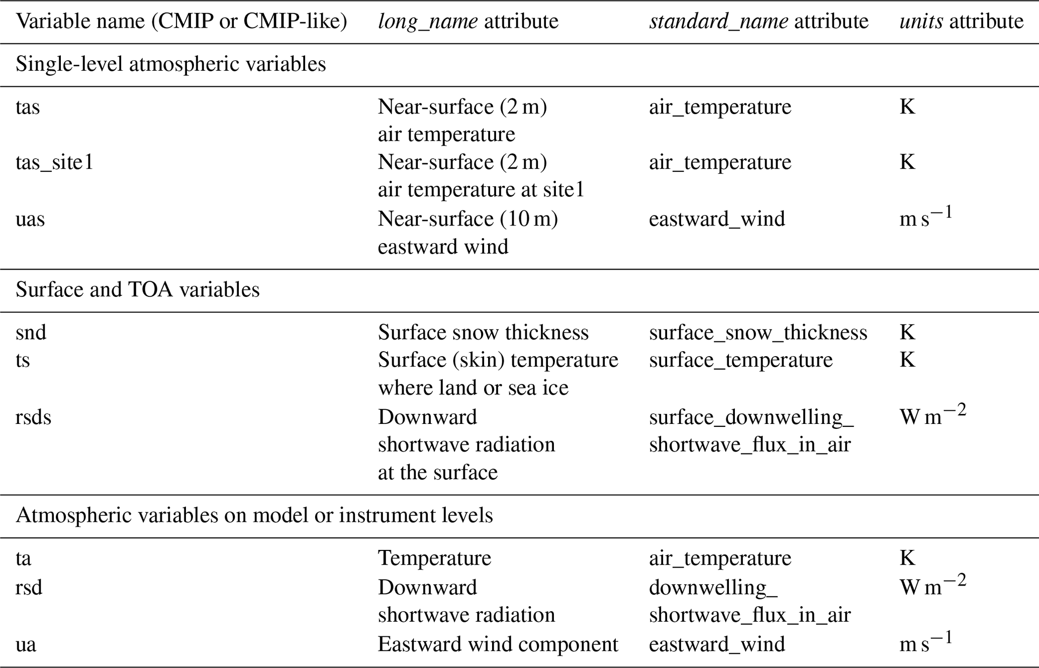
Table 4 Examples of non-atmospheric variables, together with the associated long_name, standard_name, and units attributes (extracted from Hartten and Khalsa, 2022).

Table 5 lists the other attributes that should be included in MODFs for geophysical variables. Some of the variable attributes in Table 5 are listed in the CF conventions as being for use as either global or data attributes, but the history attribute is listed as for global use only. We have encouraged its use with variables (data) in MODFs because we believe that this maintains the spirit, if not the letter, of the CF conventions; like institution, references, source, and title, history helps document the provenance and nature of the data included in these multi-institution, multi-sourced files. We also encourage MODF (and MMDF) makers to make use of additional variable attributes to share information about the variable contents with users. Brief explanations of some of the attributes in Table 5 follow, but those interested in creating MODFs should also review the definitions and explanations of attributes in the ACDD and the CF conventions.

original_name. Refers to the name of the variable in the original file from which it was extracted. This provides an important cross-reference in the case where a user may need to refer back to the original source data set.

instrument. Tracking instrumentation characteristics and, in many cases, calibration coefficients is critical to provide information for users who may be in the process of developing refined data processing, developing higher-order products, or doing instrument intercomparison studies.

references. Published material that describes either the data or the methods used to produce them should be listed here. Best practice is to include a URI (a DOI for a paper or a URL for a website).

source. Both the CF conventions and ACDD describe this as “the method of production of the original data”, by which they mean either the model that produced it or the instrument that gathered it. In either case, the idea is to give the user information that will help them understand what they're working with, including what assumptions or methods are inherent to the data. Therefore, the name and version of a numerical model or the type (and perhaps the make and model) of an instrument would be appropriate here.

history. Provides an audit trail for the data, documenting its provenance. When used as a variable attribute, this should trace what has been done to the data from its raw state until it was put into this file. We recommend that each step be documented by a line that starts with a date stamp and the version number of the variable, the person or entity who did the action, a brief description of the action, and any program(s) which accomplished the action (including relevant settings or command arguments).

Table 5 Minimum recommended additional variable attributes for geophysical variables (adapted from Hartten and Khalsa, 2022).

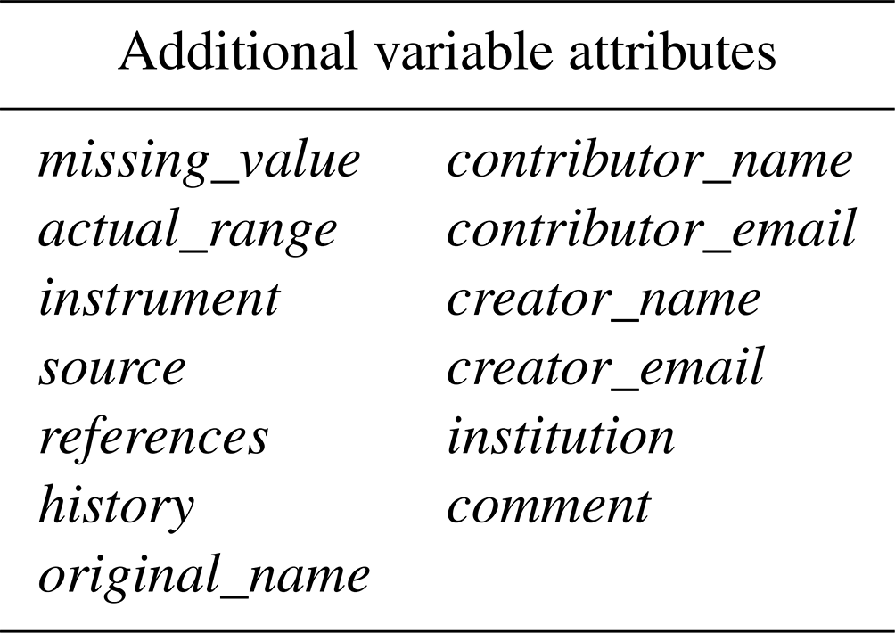
Figure 3 describes the workflow and process that developed through the efforts of the YOPPsiteMIP team of observers, modelers, data scientists, and data managers. Key components include both the H-K schema and the A-M variable and attribute template table (Morris and Akish, 2022). The A-M table was developed for collating metadata that were not already encoded into the individual data files being used as input to MODFs, and it was used as a direct input to the MODF creation process. The development of the H-K schema and the A-M table was a highly iterative process, as indicated by the two-way arrow between (c) and (d) in Fig. 3, and is expected to continue to be so.

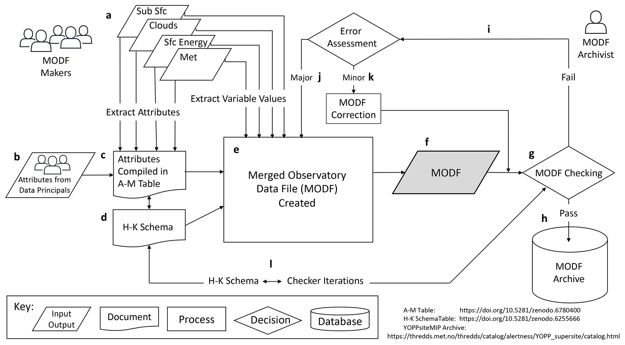
Figure 3 The MODF workflow process. (a) Gather input files. (b) Interview contributing data principals to obtain necessary metadata that are not digitally encoded in the data files. (c) Utilize the A-M MODF template to construct the specific MODF framework-based inputs from (a) and (b) compliant with the H-K schema (d). MODF makers create the MODF (e) with inputs from (c) and the data values from individual files collected (a). (f) The MODF file. (g) MODF checking. (h) Upon “pass”, send the MODF to the archive. (i) Upon “fail”, assess the MODF. (j) In the case of a major fail, return the MODF to the MODF makers. (k) In the case of a minor fail, the archivist corrects and sends the MODF to the archive after rechecking (g). (l) Iterative developments between the H-K schema (d) and MODF checking (l). The people icons were adapted from one designed by VectorStock (image #45970079 at http://VectorStock.com, last access: 22 July 2023).

6 Discussion

We have presented the H-K schema (Hartten and Khalsa, 2022) and a production framework for organizing complex campaign and observatory data from multiple instruments into Merged Observatory Data Files (MODFs). The H-K schema also enables the formatting of forecast model output into corresponding Merged Model Data Files (MMDFs). MODFs and MMDFs, i.e., Merged Data File (MDF) collections, are compliant with existing metadata and data standards that support FAIR principles. The schema and the framework were developed by a YOPPsiteMIP working group of observers, modelers, and data managers. MODFs address the mundane but complex issues that arose from the YOPPsiteMIP vision of confronting polar weather-forecasting models with observations from richly instrumented sites during special observing periods. The issues addressed include data semantics, attribution for the original data, data provenance, different cadences, multiple measurements of the same variable from the same site (including the local subgrid-scale spatial distribution), versioning strategies to account for different levels of data processing, unit conventions, and missing data indicators. Because of the high cadence of many measurements (seconds to minutes), MODFs can be used to evaluate accumulating biases at model time-step increments, which are typically shorter than model output increments.

Although providing site, instrument, processing, and attribution metadata documentation is good practice, it is often neglected. Since we discovered that this essential MODF information was difficult to assemble after the fact, we recommend that, as part of the routine MODF development process, observers use datagrams during the development, deployment, and operation of sensors as a standard practice. Datagrams “are designed to document the life story of a data value from start to finish and provide a guide for humans to design, deploy, troubleshoot, repair, record, transmit, process, and archive data collected with measuring devices.” (Morris and Uttal, 2022). In addition to proactively gathering observation metadata, the MIIP strategy would also be significantly supported if model outputs were extracted in the vicinity of observatories in real time. This can be difficult after the fact for routine output and impossible for time-step output. Furthermore, while we strongly encouraged YOPPsiteMIP MODF and MMDF makers to check their files for compliance before submitting, we have found it incredibly useful that the data manager at the host archive we worked with actively participated in checking the files (Tjernström, 2022) and, in some cases, made editorial corrections to bring the MODFs and MMDFs into full compliance with the H-K schema. This sort of effort at the data archive can be necessary when MDF providers do not have the resources to support the level of data management required to create fully compliant files.

Currently, the H-K schema includes geophysical variables across the atmosphere, snow, ice, terrestrial, and ocean systems. Appendix A lists the MODF (and MMDF) values that are currently in the H-K schema (version 1.2). These are not exhaustive, and we expect that MODF users and makers will augment their MODF files to accommodate individual campaigns by including, for example, atmospheric aerosols, constituent gases, additional ocean and terrestrial variables, and ecosystem and biogeochemical data. Any additional variables should be incorporated for specific applications using the metadata standards described here. Some MODF variable collections (e.g., precipitation from different sensor systems or profiler data with sensor- and/or range-dependent measurement volumes) may require the discovery or creation of special variable attributes. If no standard exists, we recommend that the custom variable attribute should be submitted for consideration as a standard; directions are available via the “Discussion” link in CF Metadata Conventions (2024). However, MODF makers should keep in mind that additional variable metadata for complicated variables can also be shared via the reference and comment attributes.

A first set of MODF files (Mariani et al., 2024) implementing the H-K schema from concept to production for YOPP special observing periods has been archived by the Norwegian Meteorological Service, where a collection (https://thredds.met.no/thredds/catalog/alertness/YOPP_supersite/catalog.html, last access: 4 August 2023) of matched MODF and MMDF files is available for several Arctic ground stations. As of March 2024, these MODFs are not yet available for all the Arctic YOPP supersites, nor for any of the Antarctic YOPP supersites; those which are available do not yet contain all the observed variables from the individual sites. This situation reflects the difficulty involved with amalgamating data into MODF files. An initial analysis (Day et al., 2023) using the YOPPsiteMIP MODF–MMDF collection demonstrates, through a number of examples and case studies, how process-describing variables such as surface fluxes (longwave, sensible, and latent) and ground fluxes can be used to gain a deeper understanding of the nature of forecast errors.

The main motivation for the creation of the MODF and MMDF file format is to accelerate improvements in process description in numerical models by facilitating evaluation using suitable observations. The main strength is that the concept and format are co-developed by and have a purpose for both the modeling and observational communities. Another beneficial aspect is that what we have presented here is a structure that could be built upon by the data management community and incorporated into data center operations. The format is intentionally designed with growth in mind, allowing for new variables and feature types together with the possible development of community platforms for interaction. These aspects pave the way for widening the concept to include more sites, extending the time coverage for existing sites, and including more processes and additional research areas. While the material presented here is intended to help explain MODFs and how to create them, we encourage those making MODFs to explore the ACDD, the CF conventions, and the DataCite Metadata Kernel to more fully understand the possibilities for expansion.

We acknowledge that model–observation interoperability is based on standards that may be limiting for specific applications, so we expect that custom MODFs will be developed as necessary. In other words, the MODF concept is meant to be flexible while remaining within proscribed protocols. While there are few limitations to the MODF concept, currently, the types of data that are encompassed are designed for the YOPPsiteMIP goals (Jung et al., 2024). Further development depends on the engagement of communities and their interest in growing and expanding the format based on other research needs. The success of the MODF format is and will be dependent upon the interest of those data producers.

The concept of organizing multivariate observational data sets from a single site or platform into a unified product is not unique. Wei et al. (2021) describe how the International Consortium for Atmospheric Research on Transport and Transformation (ICARTT) data format conventions (Aknan et al., 2013) can be used to create merged in situ data products based on data from research aircraft carrying multiple sensors. The US DOE ARM program (Stokes and Schwartz, 1994) creates Climate Modeling Best Estimate (CMBE) data files (Xie et al., 2010) for their climate reference sites. Hogan and O'Connor (2004) describe how the Cloudnet project preprocesses cloud data from multiple remote sensors using appropriate ancillary observations and model forecasts and then makes the output available in netCDF format with rich metadata about the preprocessing. What is unique about MODFs is the strategy of simultaneously creating corresponding matched MMDF data files to support modeling verification and process evaluations. This addresses a long-standing issue with communication silos between observing and modeling sciences (Holloway et al., 2014; Sprintall et al., 2021; Neang et al., 2021).

We also expect that MODFs will be used to facilitate studies of interdisciplinary observation-based system science. The NSF workshop report Opportunities and Challenges of Arctic System Science (Vorosmarty et al., 2018) introduced the concept of “multiple `currencies' that link the Arctic climate and environment – geophysical entities such as water, energy, carbon, and nutrients with quantifiable properties – and how they interact to produce and illuminate systems-level behaviors.” MODFs, by quantifying the currencies throughout a system with internally consistent standards, can serve to break down barriers between individual studies of separate components of the system that are typically divided along disciplinary lines, thereby advancing multidisciplinary process studies.

Generating MODFs will expand the usage of data from field campaigns by increasing data uptake and decreasing data latency. This will promote the usage of non-operational data that are currently underutilized and difficult to access comprehensively, specifically for environmental services requiring near real-time environmental intelligence. The US Interagency Arctic Research Policy Committee (IARPC) has defined environmental intelligence as “a system through which information about a particular region or process is collected for the benefit of decision makers through the use of more than one inter-related source.” Furthermore, the IARPC notes that “Traditionally, researchers collect data, develop models, and communicate results through well-established channels that are often slow and inefficient. While the vetting of scientific results ensures that the conclusions are of highest quality, the process is not well-aligned with the need for rapid information delivery in the face of environmental transitions that are putting stress on ecosystems and human populations.” MODFs will not only accelerate timely and relevant data access and scientific results for the primary researchers that collected the data; they will also support the iterative observations, modeling, and data systems that connect researchers, stakeholders, and decision makers to allow informed responses to environmental events. To this end, MODFs are designed to be living files that can be created in a timely manner with near-real-time variables and then augmented when additional variables become available. This is particularly important for situations in which observational data become obsolete before they can be utilized by environmental awareness and short-term prediction services for extreme events. MODFs can then be augmented with variables that are only available after extensive human-assisted processing (e.g., surface energy balance fluxes) for research purposes as well as with new versions of variables that require detailed quality control to produce higher-level and higher-reliability products. This addresses the concern that many data providers express about only releasing the most highly curated values (often resulting in data embargoes and release time lags) and recognizes that the level of necessary post-processing depends on the application, while still reducing the data latency so that rapid climate change events can be addressed in a timely manner.

Creating merged data products that are also findable, accessible, interoperable, and reusable is easy to say and hard to implement; it is expensive in any currency, be it time or people or computing. In developing the concept of MODFs and MMDFs, we have struggled over whether there is a realm between “nothing” and “everything”; over how to keep the quest for perfect compliance from preventing a good or even very good improvement. In the end, we think the guiding principle must be this: to remember that FAIR data are an ideal, and the implementation involves tradeoffs; some metadata is better than none, and anything that moves along this path is good.

Appendix A: Current measurable geophysical MODF and MMDF variables and their “essential climate variable” status

The H-K schema is a set of tables that is expected to be expanded and adjusted as the need arises for additional MODFs and MMDFs and for additions to existing ones. Therefore, researchers interested in using the H-K schema to guide file creation should always refer to the current online version; the DOI listed in the references of this article will always land on the most recent version of the schema, and when a new version of the H-K schema is published, the earlier versions will be prefaced with a note including a link to the latest version.

In this Appendix, we list the long_name attribute for all atmospheric (Table A1) and non-atmospheric (Table A2) geophysical variables, current as of the time of this article's submission. We do this for two reasons: to show the variety of variables incorporated into the H-K schema so far and to highlight the variables in the schema which the WMO has identified as essential climate variables (ECVs; Essential Climate Variables, 2023). Note that some of the ECVs are defined by the Global Climate Observing System (GCOS) in a manner other than the point measurements typically made at field sites. Those details are identified by footnotes in the tables. Lavergne et al. (2022) have proposed expanding the list of ECVs related to sea ice; the proposed sea ice ECVs that are in the H-K schema are separately highlighted in Table A2.

Table A1 long_name attributes of atmospheric variables (extracted from Hartten and Khalsa, 2022) that are measured at Arctic YOPP supersites or included in Arctic YOPP MMDFs (prefaced by “•”). Underlined variables are ECVs.

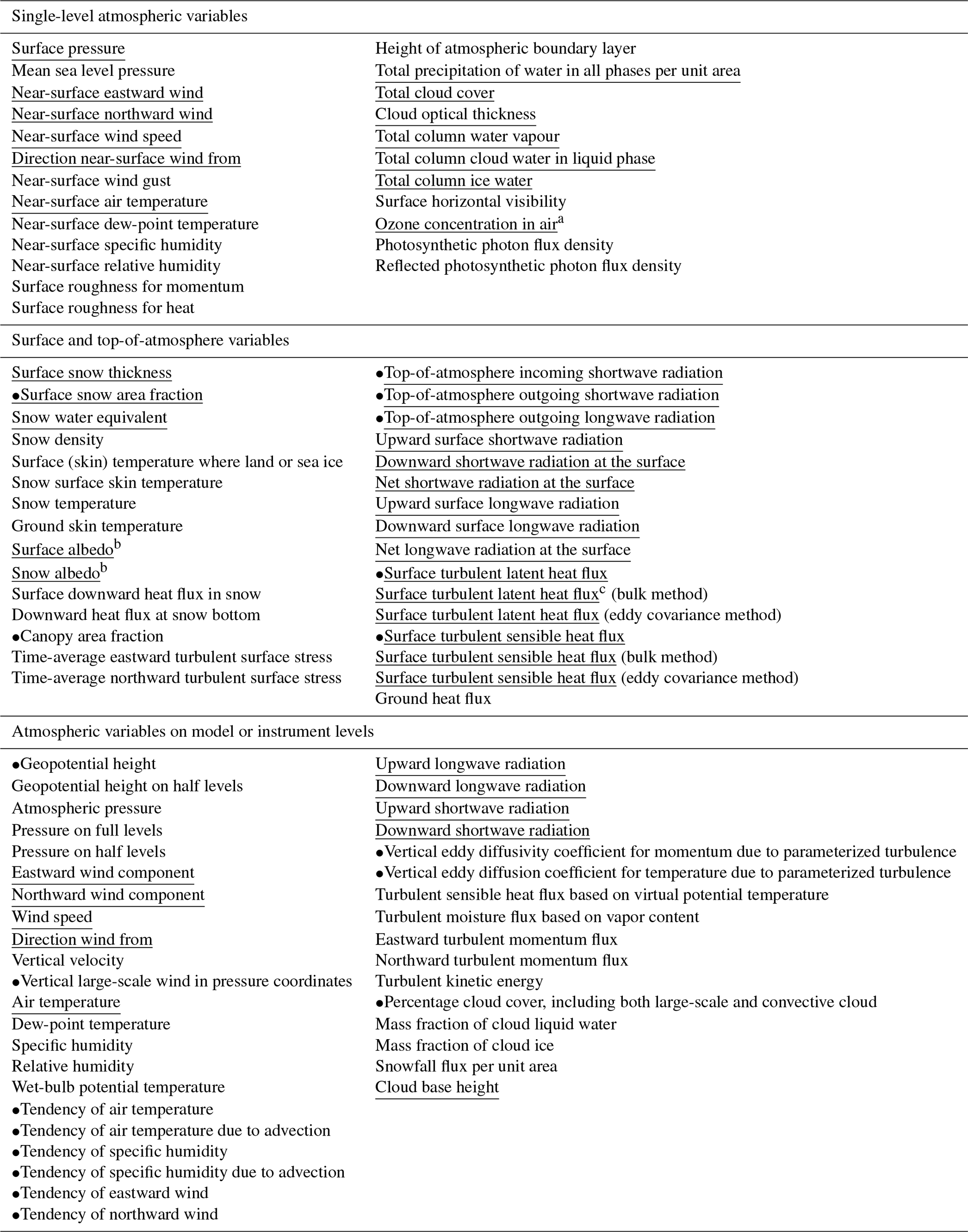
^a “Total column ozone” is the listed ECV, while observations from a site are typically point values. ^b The ECV listing is for maps, not point measurements, of albedo;
snow albedo is not explicitly listed. ^c The ECV listing specifies “land-biosphere evaporation from land”.

Table A2 Non-atmospheric variables (extracted from Hartten and Khalsa, 2022) that are measured at Arctic YOPP supersites or included in Arctic YOPP MMDFs (prefaced by “•”). Underlined variables are ECVs, with an asterisk (^∗) used for newly proposed sea ice ECVs (Lavergne et al., 2022).

^a ECV listing is for just the wave height.