RoadSurf 1.1: open-source road weather model library

Icy and snowy road conditions cause problems in many countries where temperature often drops below 0 °C. Preventive actions are necessary to keep roads ice-free and to optimize maintenance operations. Accurate road surface temperature and road condition forecasts are essential help for road maintenance crews to plan their actions. The Finnish Meteorological Institute (FMI) has produced road weather forecasts for many years with the in-house road weather model RoadSurf to aid local road authorities. Recently, FMI published an open-source road weather model library that consists of RoadSurf functions. The open publication provides an opportunity for many institutes and companies to use the library in road weather forecasting. The evaluation of the library shows that it is well suited for forecasting road surface temperature.

1 Introduction

RoadSurf is an open-source library for predicting winter road conditions. It is published under the MIT license and contains code from the Finnish Meteorological Institute's road weather model (Kangas et al., 2015), which is also named RoadSurf. In principle, it is the original RoadSurf model refactored into the library format. In this work, the model physics and algorithms are explained in detail. A model description paper of the original RoadSurf has been provided by Kangas et al. (2015), but the model has been further developed since then. Therefore, an updated model description is necessary. The newest version of the RoadSurf library is available in the FMI developers GitHub page (https://github.com/fmidev/RoadSurf, last access: 14 June 2024), and the version used in this study is available on Zenodo (Karsisto et al., 2023). Functions in the library can be used to forecast road surface temperature and the amount of water, ice, snow, and black ice on the road. Accurate predictions of road surface temperature and road conditions are important for ensuring traffic safety, minimizing the economic impacts of hazardous weather events, and maintaining efficient traffic flow. For example, with accurate surface temperature forecasts, road maintenance crews can be prepared for situations where the surface temperature drops below zero and salt the roads before ice starts to form. In addition, unnecessary salting can be avoided, resulting in economic savings. Accurate forecasts are also important to transportation and logistics, as the forecasts allow companies to optimize transportation routes and prepare for eventual disruptions to supply chains.

Several different road weather models have been developed around the world (Rayer, 1987; Yang et al., 2012; Karsisto et al., 2017). Perhaps the most used one is the open-source METRo model developed in Canada (Crevier and Delage, 2001). The development of the RoadSurf model started in the late 1990s, and its operational use started in 2000. Since then, the model has been under continuous development. For example, friction calculation and the shadowing algorithm have been added to the model (Juga et al., 2013; Karsisto and Horttanainen, 2023). The model can also be used to forecast sidewalk conditions (Hippi et al., 2020). The RoadSurf library contains the physical functions used by the RoadSurf model to predict weather road conditions. It does not contain determination of all variables predicted by RoadSurf model, such as friction and road condition (wet, icy, snowy, etc.). However, the library is designed so that each user can make their own implementation. While the RoadSurf library provides the basic prediction functions, each user can make their own additions to the model simulation. The RoadSurf library Zenodo archive provides an example implementation, which can be used as a starting point.

The functions in the RoadSurf library model the ground temperature profile and surface energy balance in one dimension. Information about atmospheric variables, such as air temperature and wind speed, is required to make the simulation. These can be obtained from the forecasts made by numerical weather prediction (NWP) models. The workings of the RoadSurf model have already been presented in several publications (Kangas et al., 2015; Karsisto et al., 2016, 2017; Karsisto and Horttanainen, 2023), but this article provides an update on the new open-source RoadSurf library. In addition, a small evaluation study is included to assess the library's performance. More extensive evaluations of the original model are provided by, for example, Karsisto et al. (2016, 2017), Toivonen et al. (2019), Hippi et al. (2020), and Karsisto and Horttanainen (2023).

The RoadSurf library can be used anywhere with the condition that weather forecast data are available. The RoadSurf model has been run for several countries in addition to Finland, including, for example, Norway, Sweden, Estonia, and the Netherlands. When implementing the model in a new area, it is important to adjust the model variables such as asphalt heat capacity and density to fit to the local conditions. The model is not optimized to predict very high road surface temperatures, so it should not be used to predict damage caused to the road by excessive heat without further studies.

The next section describes technical requirements for using RoadSurf library and the data required as model input. Section 3 explains the library physics in detail. Section 4 starts the evaluation part of the paper, with explanations of the data used and an example hindcast. Section 5 presents the actual evaluation results. Finally, Sect. 6 presents conclusions and future perspectives.

2 Requirements

The RoadSurf library is coded in Fortran 2008 and tested with GNU Fortran (GCC) 8.5.0. The library is not guaranteed to work with older Fortran compilers. As input data, the RoadSurf library requires the following input variables:

• air temperature (°C);

• dew point temperature (°C) or relative humidity (%);

• wind speed (m s⁻¹);

• precipitation intensity (mm h⁻¹);

• incoming long-wave radiation (W m⁻²);

• incoming short-wave radiation (W m⁻²).

Optional values are road surface temperature (°C) and precipitation phase (0: none; 1: rain; 2: sleet; 3: snow; 4: freezing drizzle; 5: freezing rain; 6: hail). If sky view factors (SVFs) and local horizon angles are used to modify the incoming radiation, the model also requires surface net long-wave radiation (W m⁻²) and direct solar radiation (W m⁻²) as input values. SVF describes the fraction of the radiation flux reaching the surface versus the radiation from the whole sky hemisphere. The local horizon angle means the angle between the visible horizon and the ground in a certain direction.

The atmospheric variables listed above should form a time series for the simulation duration. Although the model simulation can be done by using only either observation or forecast data, it is intended that the input data for the first part of the simulation consist of observations. This way, the ground temperature profile can evolve and form a good starting state for the actual forecast. The forecast data are necessary for forecasting the evolution of the ground temperature profile. If road surface temperature observations are available, they can be used to force the simulated surface temperature to the observations during the initialization.

As the RoadSurf library contains only functions used by the RoadSurf model, the user is responsible for creating a program that implements them. Two examples of such a program are given in the RoadSurf library GitHub repository. The repository also contains example input datasets and a user manual. The user can write their own functions to read the input data or even include the calculation of additional variables in the simulation without modifying the original library.

3 RoadSurf physics

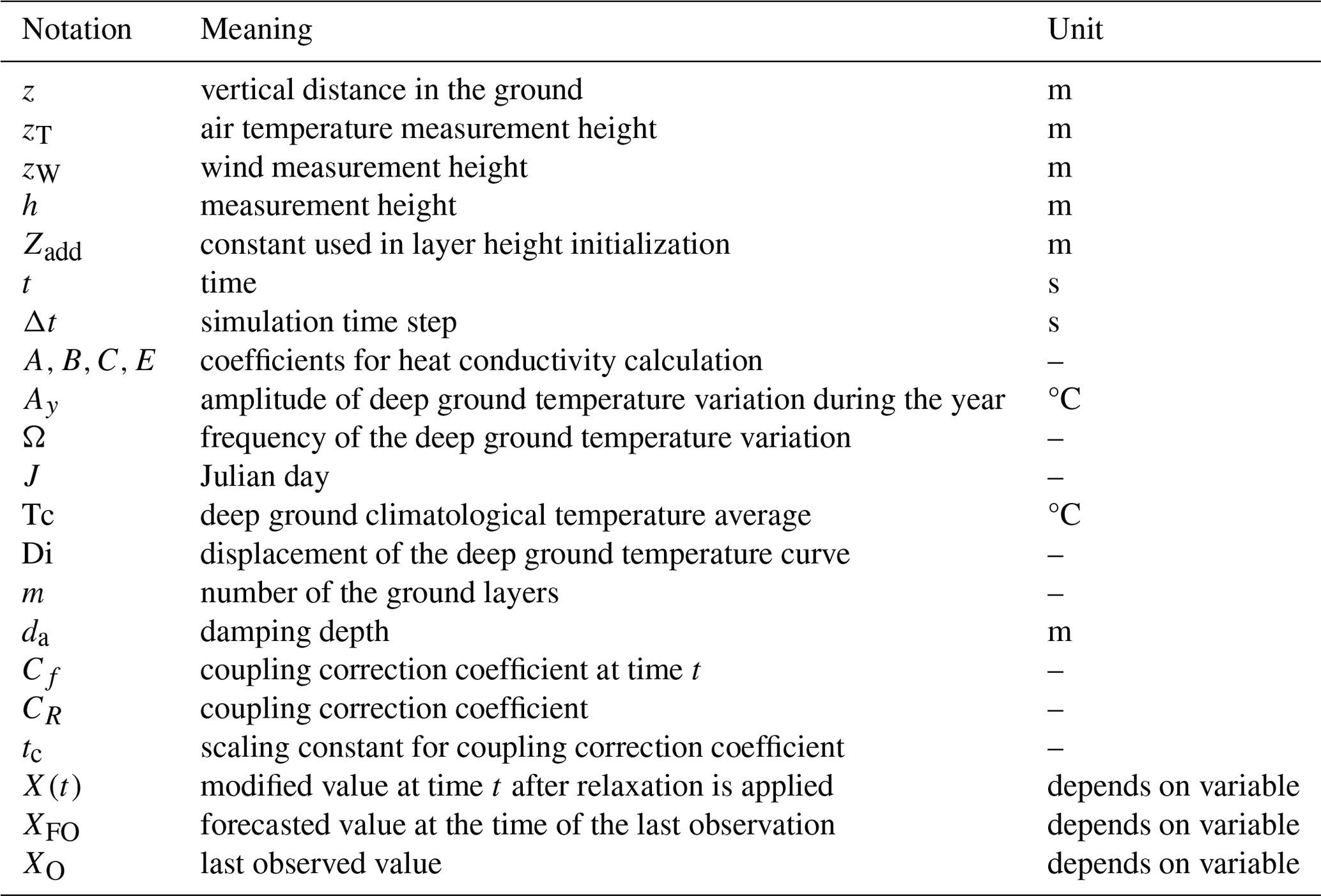
This section gives detailed explanations of the RoadSurf library physics. The notations used in this section are summarized in Appendix A for easier reference.

3.1 Surface energy balance

The most important equation in the RoadSurf library is the surface heat balance equation, which manages different energy flows in and out of the surface (Brutsaert, 1984):

$$\begin{array}{}\text{(1)}& G=R_{\mathrm{n}}-\text{LE}+H+\text{Tr},\end{array}$$

where G is ground heat flux (W m⁻²), R_n is net radiation (W m⁻²), LE is latent heat flux (W m⁻²), H is sensible heat flux (W m⁻²), and Tr is heating caused by traffic (W m⁻²).

Heating caused by traffic is just a constant value that can take on different values during daytime and nighttime. The following sections describe the calculation of ground heat flux, net radiation, latent heat flux, and sensible heat flux in detail. Figure 1 shows a schematic representation of the energy fluxes.

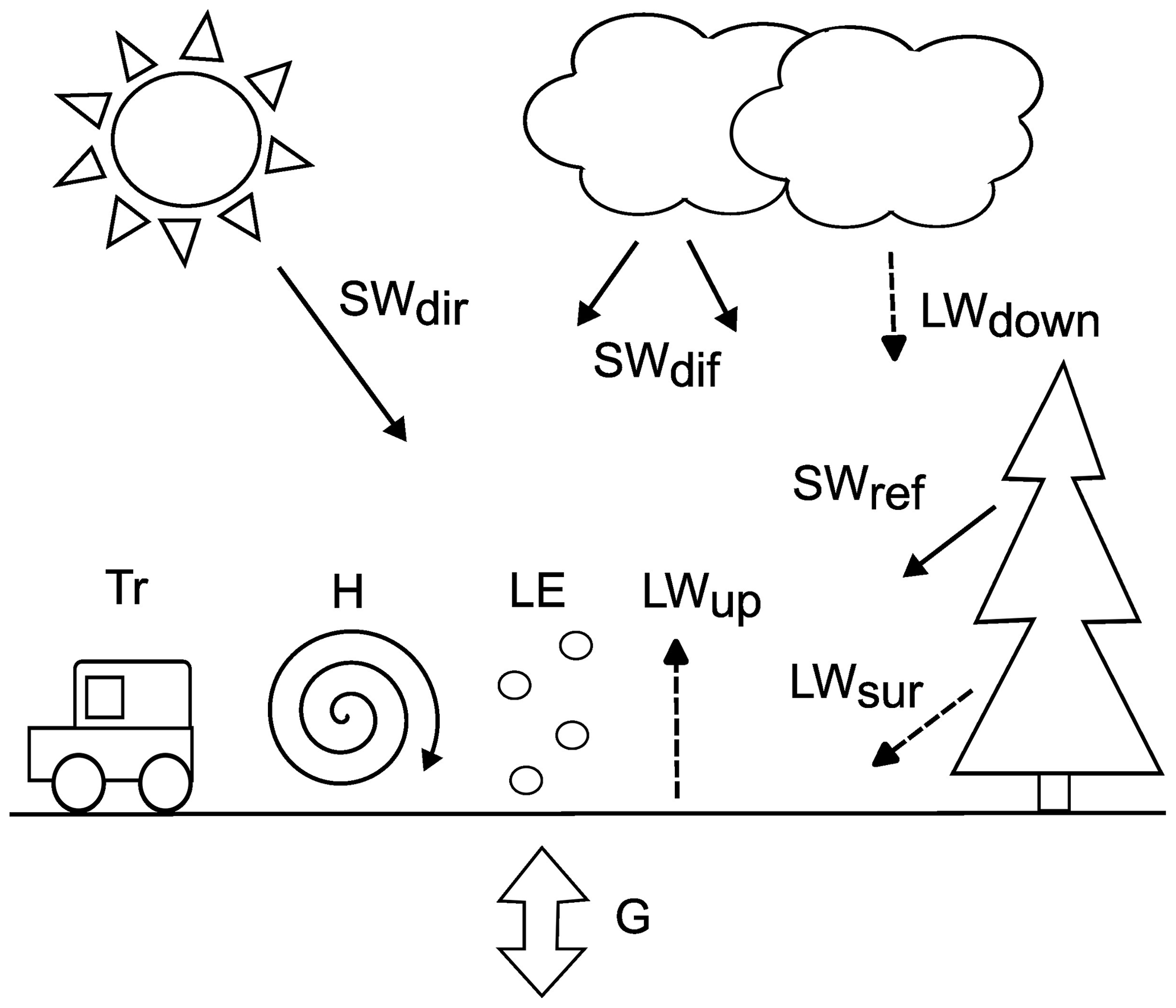
Figure 1 Schematic representation of model fluxes. SW_dir is incoming direct short-wave radiation, SW_dif is incoming diffuse short-wave radiation, LW_down is incoming long-wave radiation, Tr is traffic-induced heating, H is sensible heat flux, LE is latent heat flux, LW_up is black body emission, SW_ref is reflected short-wave radiation from the surroundings, LW_sur is long-wave radiation emitted by the surroundings, and G is ground heat flux.

3.1.1 Net radiation

Net radiation consists of incoming long-wave and short-wave radiation, black body emission from the asphalt, and reflected short-wave radiation (Brutsaert, 1984):

$$\begin{array}{}\text{(2)}& R_{\mathrm{n}}={\mathrm{SW}}_{\mathrm{down}}(\mathrm{1}-{\mathit{\alpha }}_{\mathrm{s}})+{\mathrm{LW}}_{\mathrm{down}}-{\mathrm{LW}}_{\mathrm{up}},\end{array}$$

where SW_down is incoming short-wave radiation (W m⁻²), α_s is surface albedo, LW_down is incoming long-wave radiation (W m⁻²), and LW_up is black body emission (W m⁻²).

If SVF and local horizon angles are given, they are used to modify radiation fluxes. Surrounding buildings, terrain, and vegetation reduce the amounts of incoming diffuse short-wave radiation and incoming long-wave radiation from the sky. However, they also emit some long-wave radiation and reflect short-wave radiation. SVF is used to take these effect into account. In addition, local horizon angles are used to determine whether the forecast point receives direct solar radiation (Karsisto and Horttanainen, 2023).

The input radiation values are from a numerical weather prediction model and describe values for the whole grid cell. Therefore, the net long-wave radiation or reflected solar radiation do not describe the values for a single road point well. However, when SVF is used, also the radiation from surrounding buildings, vegetation, and terrain is taken into account. The values from the numerical prediction model can be used to estimate the reflected/emitted radiation from the surrounding environment.

Diffuse solar radiation is not included in the input variables, so the amount of diffuse solar radiation is calculated as the difference between total downward short-wave radiation flux and the direct radiation flux:

$$\begin{array}{}\text{(3)}& {\mathrm{SW}}_{\mathrm{dif}}={\mathrm{SW}}_{\mathrm{down}}-{\mathrm{SW}}_{\mathrm{dir}}.\end{array}$$

SVF is used to reduce the diffuse solar radiation from the sky and to take into account the reflected solar radiation from the surrounding (Senkova et al., 2007):

$$\begin{array}{}\text{(4)}& {\mathrm{SW}}_{\mathrm{dif},\mathrm{mod}}=\text{SVF}\cdot {\mathrm{SW}}_{\mathrm{dif}}+(\mathrm{1}-\text{SVF}){\mathrm{SW}}_{\mathrm{ref}},\end{array}$$

where SW_dif,mod (W m⁻²) is modified diffuse solar radiation and SW_ref (W m⁻²) is the reflected solar radiation from surroundings. It is calculated as the sum of reflected direct solar radiation and reflected diffuse solar radiation fluxes:

$$\begin{array}{}\text{(5)}& {\mathrm{SW}}_{\mathrm{ref}}={\mathit{\alpha }}_{\mathrm{sur}}{\mathrm{SW}}_{\mathrm{dir}}+{\mathit{\alpha }}_{\mathrm{sur}}{\mathrm{SW}}_{\mathrm{dif}},\end{array}$$

where α_sur is the average albedo of the surrounding environment. The modified incoming solar radiation is then calculated as

$$\begin{array}{}\text{(6)}& {\mathrm{SW}}_{\mathrm{down}}={\mathrm{SW}}_{\mathrm{dif},\mathrm{mod}}+{\mathrm{SW}}_{\mathrm{dir}}.\end{array}$$

If local horizon angles are given, the model determines whether the point gets direct solar radiation based on the sun position. The calculation of the sun's position is based on the methods presented in the book by Jean Meeus (Meeus, 1991). If the local horizon angle in the direction of the sun is greater than the sun elevation angle, the direct solar radiation is set to zero.

SVF is used to modify the incoming long-wave radiation as (Senkova et al., 2007)

$$\begin{array}{}\text{(7)}& {\mathrm{LW}}_{\mathrm{down}}=\text{SVF}\cdot {\mathrm{LW}}_{\mathrm{down}}-(\mathrm{1}-\text{SVF}){\mathrm{LW}}_{\mathrm{sur}},\end{array}$$

where LW_sur (W m⁻²) is long-wave radiation from the surrounding vegetation, terrain, and buildings. Smaller SVF decreases the amount of long-wave radiation from the sky but increases the long-wave radiation from surroundings. As an approximation of the radiation from the surroundings, the model uses upward radiation from an NWP model. As the radiation output from an NWP model represents the whole grid cell, the upward long-wave radiation can be assumed to present the road surroundings rather than the road that covers only small part of the grid. Although upward radiation is not the same as radiation towards the road point, it can be used as a rough approximation. It is calculated as the difference between the net long-wave radiation and incoming long-wave radiation:

$$\begin{array}{}\text{(8)}& {\mathrm{LW}}_{\mathrm{sur}}={\mathrm{LW}}_{\mathrm{net}}-{\mathrm{LW}}_{\mathrm{down}}.\end{array}$$

The long-wave radiation emitted by the road is calculated as black body emission (Campbell, 1986):

$$\begin{array}{}\text{(9)}& {\mathrm{LW}}_{\mathrm{up}}=\mathit{ϵ}{\mathit{\sigma }}_{\mathrm{SB}}{T}_{\mathrm{sK}}^{\mathrm{4}},\end{array}$$

where ϵ is the emissivity factor, σ_SB is the Stefan–Boltzmann constant (W m${}^{-\mathrm{2}}{K}^{-\mathrm{4}}$), and T_sK is surface temperature (K).

3.1.2 Albedo

Albedo means the fraction of the short-wave radiation that is reflected by the surface. Both asphalt albedo and snow albedo are given to RoadSurf as input parameters. Default values are 0.1 and 0.6, respectively. Asphalt albedo is used when there is no ice, snow, or deposit on the road surface. When there is snow on the surface, the surface albedo is set to snow albedo as long as the snow storage exceeds the ice storage. When the ice storage is larger than the snow storage, the surface albedo is calculated with equation

$$\begin{array}{}\text{(10)}& {\mathit{\alpha }}_{\mathrm{s}}={\mathit{\alpha }}_{\mathrm{asp}}+{\displaystyle \frac{{\text{St}}_{\mathrm{sum},\mathrm{ice}}/\mathrm{1.5}}{{\mathit{\alpha }}_{\mathrm{snow}}-{\mathit{\alpha }}_{\mathrm{asp}}}},\end{array}$$

where α_asp is asphalt albedo, α_snow is snow albedo, and St_sum,ice is the total ice content (water equivalent millimeters). The total ice content is calculated as the sum of deposit storage and the average of the ice storage and the secondary ice storage. Secondary ice storage is explained in Sect. 3.5. If St_sum,ice is greater than 1.5 mm, the albedo is set to snow albedo.

3.1.3 Sensible heat flux

Sensible heat flux means the energy flux between air and surface. It is calculated as (Campbell, 1985)

$$\begin{array}{}\text{(11)}& H=\text{BLC}(T_{\mathrm{s}}-T_{\mathrm{a}}),\end{array}$$

where BLC is boundary layer conductance (J m⁻² s⁻¹ K⁻¹), T_s is surface temperature (°C), and T_a is air temperature (°C). Boundary layer conductance describes how easily the heat is transferred between air and surface. It is calculated as (Campbell, 1985, 1986)

$$\begin{array}{}\text{(12)}& \text{BLC}={\displaystyle \frac{c_{\mathrm{a}}{\mathit{\rho }}_{\mathrm{a}}k{u}^{*}}{\ln \left(\frac{z_{\mathrm{T}}-d+z_{\mathrm{h}}}{z_{\mathrm{h}}}\right)+{\mathrm{\Psi }}_{\mathrm{h}}}},\end{array}$$

where c_a is the specific heat of air (J kg⁻¹ K⁻¹), ρ_a is the density of dry air (kg m⁻³), k is von Karman's constant, u^* is the friction velocity (m s⁻¹), z_T is the air temperature measurement height (m), d is the zero plane displacement height (m), z_h is the surface roughness parameter for heat (m), and Ψ_h is the stability correction factor for heat (m).

An iterative process is applied to solve this equation as it cannot be solved directly because of connected variables.

c_a is dependent on air temperature and is calculated as isobaric specific heat for dry air (Garratt, 1992):

$$\begin{array}{}\text{(13)}& c_{\mathrm{a}}=\mathrm{1005}+{\displaystyle \frac{(T_{\mathrm{aK}}-\mathrm{250}{)}^{\mathrm{2}}}{\mathrm{3364}}},\end{array}$$

where T_aK is air temperature (K). Air density is calculated according to the ideal gas law:

$$\begin{array}{}\text{(14)}& {\mathit{\rho }}_{\mathrm{a}}={\displaystyle \frac{p}{R_{\mathrm{d}}{T}_{\mathrm{aK}}}},\end{array}$$

where p is pressure (Pa) and R_d is the gas constant for dry air (287.05 J kg⁻¹ K⁻¹). Pressure is not included in the input of the simulation and is assumed to always be 1000 hPa.

u^* is calculated with equation (Campbell, 1985)

$$\begin{array}{}\text{(15)}& u^{*}={\displaystyle \frac{ku}{\ln \left(\frac{z_{\mathrm{W}}-d+z_m}{z_m}\right)+{\mathrm{\Psi }}_m}},\end{array}$$

where z_W is the wind speed measurement height (m), z_m is the surface roughness parameter for momentum (m), and Ψ_m is the stability correction factor for momentum. Values for z_T, z_W, d, z_h, and z_m are given as input. Default values are z_T=2 m, z_W=10 m , d=0, z_h=0.001 m, and z_m=0.4 m.

Boundary layer stability is an important factor in the sensible heat flux calculation. Mixing is larger in unstable conditions than in a stable boundary layer. The relative importance of the thermal and mechanical turbulence in boundary layer transport is described as (Campbell, 1985)

$$\begin{array}{}\text{(16)}& \mathit{\zeta }=-{\displaystyle \frac{k{z}_{\mathrm{T}}gH}{c_{\mathrm{a}}{\mathit{\rho }}_{\mathrm{a}}{T}_{\mathrm{aK}}{u^{*}}^{\mathrm{3}}}},\end{array}$$

where g is the gravitational constant (9.81 m s⁻²). ζ is used to calculate stability correction factors. In stable conditions ζ is positive and

$$\begin{array}{}\text{(17)}& {\mathrm{\Psi }}_{\mathrm{h}}={\mathrm{\Psi }}_m=\mathrm{4.7}\mathit{\zeta }.\end{array}$$

In unstable conditions ζ is negative and

$$\begin{array}{}\text{(18)}& {\mathrm{\Psi }}_{\mathrm{h}}=-\mathrm{2}\ln \left({\displaystyle \frac{\mathrm{1}+\sqrt[\mathrm{2}]{\mathrm{1}-\mathrm{16}\mathit{\zeta }}}{\mathrm{2}}}\right)\end{array}$$

and

$$\begin{array}{}\text{(19)}& {\mathrm{\Psi }}_m=\mathrm{0.6}{\mathrm{\Psi }}_{\mathrm{h}}.\end{array}$$

Equations (18) and (19) are also used in neutral (ζ=0) conditions.

The equations above include several connected parameters, which is why BLC must be solved iteratively. First, Ψ_h and Ψ_m are set to zero and BLC, H, and ζ are calculated. Second, Ψ_h and Ψ_m are calculated using the obtained values. Then BLC, H, and ζ are calculated again using the new values. The iteration is continued until the absolute difference between two BLC values from the subsequent iteration rounds is smaller than 0.001 or the maximum amount of iterations (40) is reached.

3.1.4 Latent heat flux

Latent heat flux means the energy released in condensation or energy consumed in evaporation. It is calculated as (Calder, 1990)

$$\begin{array}{}\text{(20)}& \text{LE}={\displaystyle \frac{{\mathit{\rho }}_{\mathrm{m}}{c}_{\mathrm{a}}}{\mathit{\gamma }}}{\displaystyle \frac{e_{\mathrm{s}}-e_{\mathrm{a}}}{r_o}},\end{array}$$

where ρ_m is the density of moist air (kg m⁻³), γ is the psychrometric constant (kPa °C⁻¹), e_s is the vapor pressure at the surface (kPa), e_a is the vapor pressure of the air (kPa), and r_o is the aerodynamic resistance (s m⁻¹).

Positive latent heat flux means that water is evaporated from the surface and negative that water is condensed on the surface. In the calculation ρ_m is approximated as ρ_a. γ is dependent on air temperature and is calculated using equation developed from values in Calder (1990):

$$\begin{array}{}\text{(21)}& \mathit{\gamma }=\mathrm{0.1}\cdot (\mathrm{0.00063}{T}_{\mathrm{aK}}+\mathrm{0.47496}).\end{array}$$

Water vapor pressure at the surface is approximated as saturated water vapor pressure. Over water, this can be calculated as (Calder, 1990)

$$\begin{array}{}\text{(22)}& e_{\mathrm{s}}=\mathrm{0.61078}{e}^{\mathrm{17.269}{T}_{\mathrm{s}}/(T_{\mathrm{s}}+\mathrm{237.3})}\end{array}$$

and over ice as

$$\begin{array}{}\text{(23)}& e_{\mathrm{s}}=\mathrm{0.61078}{e}^{\mathrm{21.875}{T}_{\mathrm{s}}/(T_{\mathrm{s}}+\mathrm{265.5})}.\end{array}$$

In the air, the water vapor pressure is calculated from the saturated vapor pressure as

$$\begin{array}{}\text{(24)}& e_{\mathrm{a}}={\displaystyle \frac{\text{RH}}{\mathrm{100}}}\cdot e_{\mathrm{s}},\end{array}$$

where RH is relative humidity (%). In unstable conditions, aerodynamic resistance can be calculated as (Tourula and Heikinheimo, 1998)

$$\begin{array}{}\text{(25)}& r_o={\displaystyle \frac{\left(\ln \left(\frac{h-d}{z_m}\right)+\mathrm{\Psi }\right)\left(\ln \left(\frac{h-d}{z_{\mathrm{h}}}\right)+\mathrm{\Psi }\right)}{k^{\mathrm{2}}u}},\end{array}$$

where h is measurement height (m) and $\mathrm{\Psi }={\mathrm{\Psi }}_m={\mathrm{\Psi }}_{\mathrm{h}}$. However, the RoadSurf library uses modified version of this equation:

$$\begin{array}{}\text{(26)}& r_o={\displaystyle \frac{\left(\ln \right(\frac{z_{\mathrm{W}}+z_m}{z_m})+{\mathrm{\Psi }}_m)\left(\ln \right(\frac{z_{\mathrm{W}}+z_{\mathrm{h}}}{z_{\mathrm{h}}})+{\mathrm{\Psi }}_{\mathrm{h}})}{k^{\mathrm{2}}u}}.\end{array}$$

Ψ_m and Ψ_h are not considered to be equal as in Tourula and Heikinheimo (1998), where stability correction was marked simply as Ψ. In addition, zero plane displacement is assumed to be small, but surface roughness for momentum is added to the equation. The aerodynamic resistance has maximum limit of 30 s m⁻¹. The difference between Eqs. (25) and (26) causes only slight differences in aerodynamic resistance, so the modifications do not have much effect. Equation (26) is used also in stable conditions in the simulation for simplicity. As water vapor pressure in Eq. (20) is always estimated as saturated vapor pressure, LE can be positive even when there is no water on the surface. In the simulation, LE is set to zero if there is no water to evaporate and LE is positive.

3.2 Heat flow in the ground

The ground is divided into several layers for the heat flow calculation. The number of layers is 16. The heat transfer between the layers is based on equation (Patankar, 1980)

$$\begin{array}{}\text{(27)}& {\mathit{\rho }}_{\mathrm{g}}{c}_{\mathrm{g}}{\displaystyle \frac{\partial T(z,t)}{\partial t}}={\displaystyle \frac{\partial }{\partial z}}K{\displaystyle \frac{\partial T(z,t)}{\partial z}},\end{array}$$

where T is the ground layer temperature (°C), z is the vertical distance in the ground (m), t is time (s), K is heat conductivity (W m⁻¹ K⁻¹), ρ_g is the density of the ground (kg m⁻³), and c_g is the specific heat capacity of the ground (J kg⁻¹ K⁻¹).

After integrating over the volume of the layer and time step, the equation is discretized and solved with the forward difference explicit method. This results in the following equation (Campbell, 1985):

$$\begin{array}{}\text{(28)}& \begin{array}{rl}{T}_i^{j+\mathrm{1}}& =T_i+{\displaystyle \frac{\mathrm{1}}{{\mathit{\rho }}_{\mathrm{g}}{c}_{\mathrm{g}}\frac{z_{i+\mathrm{1}}-z_{i-\mathrm{1}}}{\mathrm{2}\mathrm{\Delta }t}}}\left(K_i{\displaystyle \frac{T_{i+\mathrm{1}}^j-T_i^j}{z_{i+\mathrm{1}}-z_i}}\right.\\ & \left.-K_{i-\mathrm{1}}{\displaystyle \frac{T_i^j-T_{i-\mathrm{1}}^j}{z_i-z_{i-\mathrm{1}}}}\right).\end{array}\end{array}$$

The index j refers to the time step and index i to the number of the ground layer. This equation is used to calculate temperature for each layer at each time step. The output surface temperature given by the model is calculated as the average temperature of the first two layers, because it matches better to the observations than the temperature of the topmost layer. The user can also set the height for which the output temperature is interpolated. The average surface temperature is often used in library functions for heat flow and storage term calculation instead of the temperature of the topmost layer.

3.2.1 Volumetric heat capacity and heat conductivity

Water in the ground is taken into account in the heat capacity calculation. The volumetric heat capacity of the ground (ρ_gc_g) is calculated as a weighted average of the dry ground and water volumetric heat capacities:

$$\begin{array}{}\text{(29)}& {\mathit{\rho }}_{\mathrm{g}}{c}_{\mathrm{g}}=(\mathrm{1}-\mathit{\varphi }){\mathit{\rho }}_{\mathrm{s}}{c}_{\mathrm{s}}+\mathit{\varphi }{\mathit{\rho }}_{\mathrm{w}}{c}_{\mathrm{w}},\end{array}$$

where ρ_gc_g is the volumetric heat capacity of wet ground (J m⁻³ K⁻¹), ρ_sc_s is the volumetric heat capacity of dry ground (J m⁻³ K⁻¹), ρ_wc_w is the volumetric heat capacity of water (J m⁻³ K⁻¹), and ϕ is the porosity of the ground.

Porosity means the fraction of empty spaces in the ground. The values are given as input to the library.

Water density and specific heat capacity are considered temperature dependent when water temperature is above 0 °C. They are calculated with equations that are derived from tables presented in Campbell (1986) and Weast (1975):

$$\begin{array}{}\text{(30)}& {\displaystyle }{\mathit{\rho }}_{\mathrm{w}}\left(T_{\mathrm{w}}\right)=-\mathrm{0.0050}{T}_{\mathrm{w}}^{\mathrm{2}}+\mathrm{0.0079}{T}_{\mathrm{w}}+\mathrm{1000.0028}\text{(31)}& {\displaystyle }\begin{array}{rl}{c}_{\mathrm{w}}\left(T_{\mathrm{w}}\right)& =\mathrm{1.02}\times {\mathrm{10}}^{-\mathrm{5}}{T}_{\mathrm{w}}^{\mathrm{4}}-\mathrm{1.7169}\times {\mathrm{10}}^{-\mathrm{3}}{T}_{\mathrm{w}}^{\mathrm{3}}\\ & +\mathrm{0.11516}{T}_{\mathrm{w}}^{\mathrm{2}}-\mathrm{3.4739}{T}_{\mathrm{w}}+\mathrm{4217.2},\end{array}\end{array}$$

where ρ_w is water density (kg m³), c_w is the specific heat capacity of water (J kg⁻¹ K⁻¹), and T_w is water temperature (°C).

Below 0 °C, ρ_w and c_w are set to the values of ice density and specific heat capacity of ice (Oke, 1987):

$$\begin{array}{c}{\displaystyle }{\mathit{\rho }}_{\mathrm{w}}=\mathrm{920}\mathrm{kg}{\mathrm{m}}^{-\mathrm{3}},\\ {\displaystyle }{c}_{\mathrm{w}}=\mathrm{2100}\mathrm{J}{\mathrm{kg}}^{-\mathrm{1}}{\mathrm{K}}^{-\mathrm{1}}.\end{array}$$

Heat conductivity in the ground is calculated as (Campbell, 1985)

$$\begin{array}{}\text{(32)}& \mathit{\lambda }=A+B\mathit{\theta }-(A-D)e^{-(C\mathit{\theta }{)}^E},\end{array}$$

where θ is the volumetric water content.

Coefficients A–E depend on the density of the ground (Campbell, 1985):

$$\begin{array}{}\text{(33)}& {\displaystyle }A=\mathrm{0.65}-\mathrm{0.78}{\mathit{\rho }}_{\mathrm{g}}+\mathrm{0.60}{\mathit{\rho }}_{\mathrm{g}}^{\mathrm{2}},\text{(34)}& {\displaystyle }B=\mathrm{1.06}{\mathit{\rho }}_{\mathrm{g}},\text{(35)}& {\displaystyle }C=\mathrm{1}+(\mathrm{2.6}/\sqrt{m_{\mathrm{c}}}),\text{(36)}& {\displaystyle }E=\mathrm{4},\end{array}$$

where m_c is the clay fraction of the ground.

3.2.2 Temperature field and layer height initialization

The ground is divided into 16 layers in the model. The layer thickness grows towards the bottom according to the formula

$$\begin{array}{}\text{(37)}& {\displaystyle }{Z}_{i+\mathrm{1}}=Z_i+\mathrm{0.01442}(i-\mathrm{1})+Z_{\mathrm{Add}},\text{(38)}& {\displaystyle }Z\left(\mathrm{1}\right)=\mathrm{0},\end{array}$$

where Z_i+1 (m) is the distance of the layer i midpoint from the surface and Z_Add (m) is constant. The temperature of the layers 1–4 is set to the observed surface temperature at the initialization. If observations are not available, the temperature of the ground layers 1–4 is set to the air temperature. The temperature of the lowest layer depends on the time of the year according to the equation (Monteith and Unsworth, 2013)

$$\begin{array}{}\text{(39)}& T_{m+\mathrm{1}}={\text{Tc}}_{m+\mathrm{1}}+A_y\sin \left(\mathrm{\Omega }J+\mathrm{\Omega }\text{Di}-{\displaystyle \frac{Z_{m+\mathrm{1}}}{d_{\mathrm{a}}}}\right),\end{array}$$

where A_y is the amplitude of variation during the year (°C), Ω is the frequency of the variation $(\mathrm{2}\mathit{\pi }/\mathrm{365})$, J is the Julian day, Tc is the climatological temperature average (°C), Di is the displacement of the curve, m is the number of the ground layers, and d_a is the damping depth. The example implementations uses Tc=6.4 °C, A_y=0.6, $\text{Di}=-\mathrm{170}$, and d_a=2.7.

The temperature of the layers between the fourth layer and the bottom layer are initialized so that the temperature change is linear with depth.

3.3 Coupling

The coupling method can be used to improve the forecast during the first forecast hours (Crevier and Delage, 2001; Karsisto et al., 2016). It is based on adjusting the amount of incoming radiation in the model. The model simulation consists of two phases. The first is the initialization phase, where the model is run with observation data. Radiation observations are often missing, so radiation data are taken from the past forecast data. After the initialization phase there is a forecast phase, where the model is run with forecast data. If road surface temperature observations are available, the temperature of the first two layers is set to the observed surface temperature during initialization.

The coupling phase in the simulation consists of the 3 h before the start of the actual forecast phase. During the coupling phase, the simulated surface temperature is not forced to the observed surface temperature as in the initialization phase. At the end of the coupling phase, the model checks whether the simulated surface temperature fits the latest observed surface temperature. If not, the model adjusts a radiation correction coefficient that modifies the incoming radiation and the simulation goes back 3 h. If the simulated surface temperature is too cold, the coefficient is increased, and if the simulated surface temperature is too warm, the coefficient is decreased. The model runs the 3 h period again and compares the new simulated surface temperature to the observation. This is continued until the simulated surface temperature is within ±0.1 °C from the observed surface temperature. Then, the simulation moves to the actual forecast phase. The radiation correction coefficient is used in the forecast phase so that it gradually approaches one as the forecast advances. The used coefficient is calculated as

$$\begin{array}{}\text{(40)}& C_f\left(t\right)=\mathrm{1.0}+C_R{e}^{-\frac{t}{t_{\mathrm{c}}}},\end{array}$$

where C_f is the correcting coefficient at time t, C_R is the original coefficient, and t_c=4 h is a scaling constant. A more detailed explanation about the algorithm that determines the coupling coefficient can be found in the user manual.

3.4 Relaxation

When the simulation switches from the observation phase to the forecast phase, there can be considerable jumps in air temperature, relative humidity, and wind speed values as forecast data differ from observation data. Relaxation makes this transition smoother by modifying these values in the forecast phase with equation

$$\begin{array}{}\text{(41)}& X\left(t\right)=X_F\left(t\right)-\left(X_{\mathrm{FO}}\right(t)-X_{\mathrm{O}})e^{-\frac{t}{t_{\mathrm{c}}}},\end{array}$$

where X(t) is the forced value at time t, X_FO is the forecasted value at the time of the last observation, and X_O is the last observed value. t_c is the same scaling constant as in Eq. (40). Relaxation can be turned on or off.

3.5 Storage terms

Storage terms in the RoadSurf library refer to the amounts of snow, ice, water, and deposit on the road (Kangas et al., 2015). The amounts are calculated in water equivalent millimeters. Deposit means black ice that has formed on the road surface via deposition. Unlike the surface temperature calculation, where the model uses clear physical definitions, the storage term calculation contains more approximations and simplifications. There are two separate storages for ice that are otherwise similar, but the secondary ice storage is reduced faster by traffic. The secondary ice storage is included in the simulation output. Water storage consists partly of the water in the asphalt pores and partly of the water on the surface. Water is considered to be only in the pores until water storage exceeds the maximum porous water content, which is given as an input parameter. The default value is 1.0 mm.

Table 1 Events that increase (+) or decrease (−) different storage terms. No sign means that the event does not affect that specific storage.

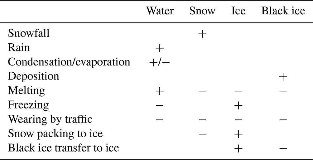
Table 1 shows which events increase or decrease the storage terms. Wearing by traffic reduces all storage terms gradually. Passing vehicles compress snow, and with time snow storage is transferred to ice storage. Black ice is transferred to ice storage when there is snow on the road, as black ice is assumed to exist only in snow-free situations.

3.5.1 Precipitation

The RoadSurf library uses three types of precipitation: water, sleet, and snow. When precipitation type is given as input, drizzle, rain, freezing drizzle, and freezing rain are classified as water. Hail is classified as snow. Water type precipitation increases the water storage, and snow type precipitation increases snow storage. If precipitation type is sleet, half of the precipitation goes to the water storage and half to the snow storage.

If precipitation type is not given, RoadSurf uses following equation to determine the type (Koistinen and Saltikoff, 1999):

$$\begin{array}{}\text{(42)}& P_{\mathrm{rain}}={\displaystyle \frac{\mathrm{1}}{\mathrm{1}+e^{P_{\exp }}}},\end{array}$$

where $P_{\exp }=\mathrm{22}-\mathrm{2.7}{T}_{\mathrm{a}}-\mathrm{0.2}$RH. If P_rain<0.3 precipitation is categorized as snow. When P_rain>0.7, precipitation is categorized as water, and when $\mathrm{0.3}\le P_{\mathrm{rain}}\le \mathrm{0.7}$, precipitation is categorized as sleet.

The storage terms have maximum limits that they cannot exceed. The default maximum limit for snow is 100 mm, for ice 50 mm, for deposit 2 mm, and for surface water 1 mm. Ice and water content are simply limited to the maximum amount, but snow storage is halved if it reaches the maximum amount. If deposit exceeds the maximum limit, excess deposit is turned to water.

3.5.2 Wear

Passing vehicles cause water, snow, and ice to gradually wear off from the road. RoadSurf has separate wear factors for each storage term that determine how fast they are reduced. The reduced amount in one time step can be calculated as

$$\begin{array}{}\text{(43)}& {\text{Wear}}_x={\text{Wf}}_x\cdot {\text{St}}_x\cdot \mathrm{\Delta }t/\mathrm{3600}\mathrm{s},\end{array}$$

where Wf_x is the wear factor for storage x, St_x is storage x (water equivalent millimeters), and Δt is time step (s). The wear factors for different storages are

Wf_snow=0.45, Wf_ice=0.319, Wf_ice2=2.552, Wf_deposit=1.16, and Wf_water=0.145.

ice2 refers to secondary ice storage and deposit to black ice. Wearing simply reduces the amount of ice, deposit, and water on each time step during the simulation. However, part of the reduced snow storage is transformed to ice. This part is calculated by multiplying the reduced amount of snow by 0.556. Snow wear is greater when the snow storage is less than 0.2 mm. In that case, snow wear is multiplied by 3. To avoid wearing becoming too small, Wf_x⋅St_x for the snow, ice and deposit wears have a minimum value of 0.01 mm and Wf_water⋅St_water has minimum value of 0.06 mm. Deposit wear has an effect only in snow-free conditions. If St_snow>0, then Wf_deposit=0.

Water wear is set to zero if the amount of water is less than one-tenth of the maximum porous water content. If the water content is less than 90 % of the porous water content, the water wear is reduced by half.

3.5.3 Evaporation and condensation

The amount of evaporated or condensed water in time each step is calculated with equation

$$\begin{array}{}\text{(44)}& {\text{EV}}_{\mathrm{w}}={\displaystyle \frac{\text{LE}}{E_{m^{\mathrm{3}}}}}\mathrm{\Delta }t,\end{array}$$

where $E_{m^{\mathrm{3}}}$ (J) means the amount of energy needed to evaporate 1 m³ of water. It is calculated as

$$\begin{array}{}\text{(45)}& E_{m^{\mathrm{3}}}=L_{\mathrm{wat}}{\mathit{\rho }}_{\mathrm{w}},\end{array}$$

where L_wat is the latent heat of water vaporization (J kg⁻¹) and ρ_w is the density of water (kg m⁻³). Water is evaporated when LE is positive and condensed when LE is negative. Snow, ice, and deposit storages must be zero and surface temperature should be at least 0.25 °C for evaporation or condensation to occur in the simulation. If the water storage is less than the maximum porous water content, the evaporated amount of water is reduced by the pore resistance factor. This factor can be set by the user but is by default 1.0, which means it has no effect.

Deposit storage is increased by deposition. It is calculated similarly to condensation, but latent heat of evaporation is replaced by latent heat of sublimation in Eq. (45). Sublimation is not taken into account in the simulation.

3.6 Freezing and melting

Freezing happens in the simulation instantly when the surface temperature goes below the freezing limit. When freezing occurs, the entire water storage is added to the ice storage and water storage is set to zero. Freezing does not affect surface temperature in the simulation, and heat released by it is not taken into account. This may cause surface temperature that is too cold and ice formation that is too fast in the simulation. However, the phenomena's accurate modeling is difficult as it would require increasing surface temperature when freezing, which would cause temperature to rise above the freezing limit. This might cause surface temperature to bounce above and below the freezing limit during freezing.

Melting transforms ice, snow, and deposit storages into water storage. The entire deposit storage is simply added to the water storage when the surface temperature goes above the melting limit. The melting of ice and snow is slower in the simulation. The amount of melted snow and ice in one time step is calculated as

$$\begin{array}{}\text{(46)}& {\text{Me}}_{\mathrm{snow}}=\mathrm{1000}{\displaystyle \frac{Q_{\mathrm{melt}}\mathrm{\Delta }t}{L_{\mathrm{melt}}{\mathit{\rho }}_w}},\end{array}$$

where Q_melt is the energy that is available for melting (J) and L_melt is the latent heat for melting (J kg⁻¹). The available energy for melting is considered the same as the energy that would be released if the surface cooled to the melting temperature. It is calculated as

$$\begin{array}{}\text{(47)}& Q_{\mathrm{melt}}={\mathit{\rho }}_{\mathrm{g}}{c}_{\mathrm{g}}{\displaystyle \frac{z_{\mathrm{2}}-z_{\mathrm{1}}}{\mathrm{2}\mathrm{\Delta }t}}(T_{\mathrm{1}}-T_{\mathrm{melt}}),\end{array}$$

where z₁ is the depth of the uppermost ground layer (m), z₂ is the depth of the second ground layer (m), T₁ is the temperature of the uppermost ground layer (J kg⁻¹), and T_melt is the melting temperature (°C). After calculating the available energy, the temperature of the two uppermost layers is set to the melting temperature + 0.01 °C. The melted amount is removed from the ice/snow storage and added to the water storage. If surface temperature warms up on the next time step, the heat is again used for melting and temperature of the two uppermost layer is again set to the melting temperature +0.01 °C. This continues until the ice and snow storages are melted entirely. If the available energy is more than is needed to melt the whole ice or snow storage in one time step, the surface is not cooled to the melting temperature but remains warmer. The energy needed to melt the whole storage is calculated as

$$\begin{array}{}\text{(48)}& Q_{\mathrm{all}}={\displaystyle \frac{L_{\mathrm{melt}}{\mathit{\rho }}_{\mathrm{w}}\frac{{\text{St}}_x}{\mathrm{1000}}}{\mathrm{\Delta }t}},\end{array}$$

where St_x is snow storage in water equivalent millimeters if there is snow on the road and ice storage if there is ice but not snow. The leftover energy can be calculated simply as the difference between Q_melt and Q_all. The temperature for the uppermost layer is then calculated as

$$\begin{array}{}\text{(49)}& T_{\mathrm{1}}=T_{\mathrm{melt}}+{\displaystyle \frac{Q_{\mathrm{melt}}-Q_{\mathrm{all}}}{(\mathit{\rho }c{)}_{\mathrm{g}}\frac{z_{\mathrm{2}}-z_{\mathrm{1}}}{\mathrm{2}\mathrm{\Delta }t}}}.\end{array}$$

The temperature of the second layer is still set to T_melt+0.01 °C.

The melting process is not entirely physically correct as the same energy is used to melt both snow and ice storages, and Q_all includes only ice or snow storage, but the method can still be used to approximate the melting process.

Snow can also be transferred instantly to water if the water content is high enough compared to the snow content. The water-to-snow ratio is calculated as

$$\begin{array}{}\text{(50)}& {\text{WS}}_{\mathrm{rat}}={\text{St}}_{\mathrm{water},\mathrm{surf}}/({\text{St}}_{\mathrm{water},\mathrm{surf}}+{\text{St}}_{\mathrm{snow}}),\end{array}$$

where St_water,surf (mm) is the part of water storage that is not located in the asphalt pores. If the water-to-snow ratio is larger than 0.6, snow is transferred to water instantly. Snow and water can also turn instantly to ice in the simulation if the snow is wet. When the water-to-snow ratio exceeds 0.1 and the surface temperature drops below the freezing limit, both water and snow storage are converted into ice storage.

4 Data

4.1 Forecast

Operational weather forecasts produced by Finnish Meteorological Institute (FMI) were used as input to the road weather model to generate road weather hindcasts. The operational weather forecast is generated by the Smartmet nowcast system (Ylhäisi et al., 2017). It is a combination of a radar-based nowcast, a high-resolution NWP MetCoOp (Meteorological Cooperation on Operational NWP) nowcast, and an operational forecast edited by the on-duty meteorologist. The nowcast range (0–6 h) is updated once an hour, whereas the meteorologist-edited forecast is updated twice a day.

The radar-based nowcast is generated with the FMI Probabilistic Precipitation Nowcasting system (FMI-PPN, https://github.com/fmidev/fmippn-oper/, last access: 14 June 2024). It uses the pysteps ensemble prediction system (Pulkkinen et al., 2019) to generate the ensemble forecast from radar data. The final precipitation nowcast is a weighted average of the ensemble members generated from perturbed radar data and the control forecast generated from non-perturbed data (Ylhäisi et al., 2017). The MetCoOp nowcast model is based on the convection-permitting Applications of Research to Operations at Mesoscale (AROME) model (Seity et al., 2011). Its horizontal resolution is 2.5 km, and it is run once an hour. The forecast length is 9 h. The meteorologists at FMI use the SmartMet workstation editing tool (https://github.com/fmidev/smartmet-workstation, last access: 14 June 2024) to edit the NWP forecast. The meteorologist can select the base forecast from several different options: ECMWF's high-resolution forecast, the MetCoOp Ensemble Prediction System's (MEPS) control member, and the National Centers for Environmental Prediction (NCEP) Global Forecast System (GFS) forecast. Optionally, they can use a mix of several forecasts. The FMI also has different options of post-processed data to use as a base forecast. One is based on model output statistics (MOS) (Ylhäisi et al., 2017; Glahn and Lowry, 1972), and the other blends different models (Fritsch et al., 2000; Woodcock and Engel, 2005). After selecting the base model or models, the meteorologist can edit the forecast based on their experience, for example, by making certain areas warmer or cooler. The horizontal resolution of the edited data is about 7.5 km, and the forecast length is 10 d.

The above-mentioned data sources are blended together to create a seamless forecast for 10 d, in which the first hours consist of nowcast data and the rest of the meteorologist-edited forecast. However, the hindcasts generated in this study used only the first 24 h of the forecast data. Because the data are in gridded format, the forecast data were interpolated to the road weather station points by using bilinear interpolation except for the precipitation phase, which was taken from the nearest point instead.

4.2 Road weather observations

Intelligent Traffic Management Finland maintains approximately 400 road weather stations in Finland (Fig. 2). Their data were used in the initialization of the road weather simulations and in the evaluation of the road surface temperature forecasts. The used variables measured by the stations were air temperature, relative humidity, wind speed, precipitation intensity, and road surface temperature. Road surface temperature is measured with either an asphalt-embedded Vaisala DRS511 or an optical Vaisala DST111 (Vaisala, 2021). Some road weather stations have multiple sensors, but only one sensor from each station was used. The observation frequency is usually about 5–10 min. The observations went through simple quality check routines before using them in the initialization and verification. First, air temperature, road surface temperature, dew point temperature, relative humidity, and wind speed values that remained constant for 10 or more consecutive observations were removed. Second, spikes were removed from the air temperature, road surface temperature, and dew point temperature observations by checking if the difference between two consecutive observations was more than 5 °C and whether there were two of those kinds of changes within four consecutive observations. Third, the values that were greater than 50 °C or lower than −50 °C were removed from the air temperature, road surface temperature, and dew point temperature observations. This might have caused the removal of some real data, but it is not expected to considerably affect the results. The road weather station observations and forecast data are available in the FMI research data repository METIS (Karsisto, 2023b).

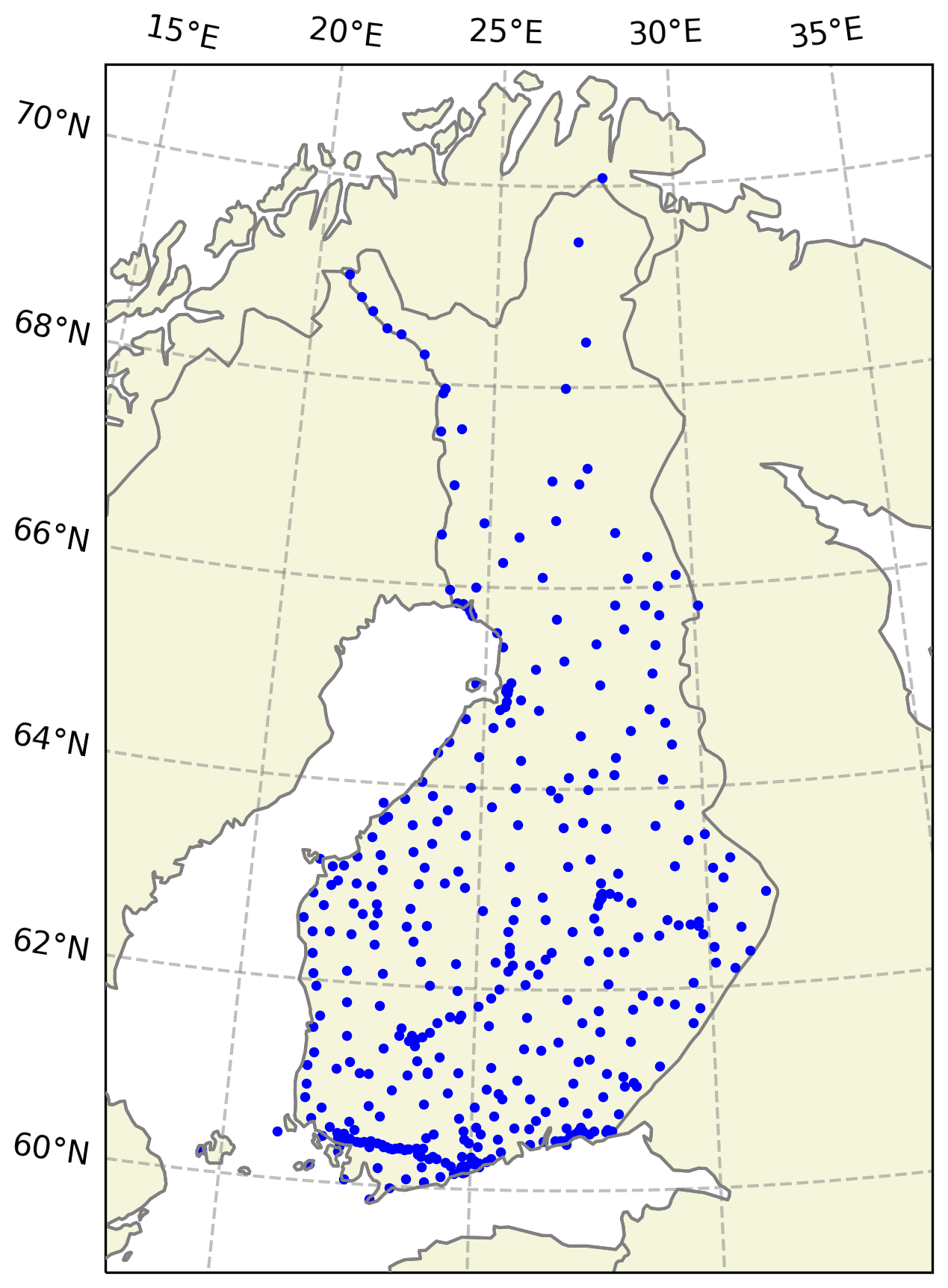
Figure 2 Geographical locations of road weather stations in Finland operated by Intelligent Traffic Management Finland. Made with Natural Earth (https://www.naturalearthdata.com/, last access: 14 June 2024).

4.3 Simulation data structure

To evaluate the performance of the RoadSurf library, it was used to make simulations with historical data. These hindcasts were done for the time period from 1 October 2022 to 31 May 2023. The used program that implemented the RoadSurf functions and did the actual simulations can be found in the GitHub repository as “Example 2” in the examples folder (https://github.com/fmidev/RoadSurf/tree/master/examples/example2, last access: 14 June 2024). To get a good starting state for the ground temperature profile, the simulations done with the RoadSurf library were first run for 48 h with observation data. However, incoming long-wave and short-wave radiation were obtained from the latest available forecast during the initialization phase due to the lack of radiation observations. After the initialization, the simulation was run 24 h with forecast data. The hindcast starting times were 00:00, 06:00, 12:00, and 18:00 UTC (universal coordinated time) each day. The local time in Finland is UTC+2 h in winter and UTC+3 h when daylight saving time is in effect. For each hindcast, the latest operational forecast that would have been available at that time was selected as the forecast data. Due to technical issues forecasts were missing for the time period from 25 December, 02:00 UTC, to 26 December, 20:00 UTC. Hindcasts starting during that period were removed from the studied data.

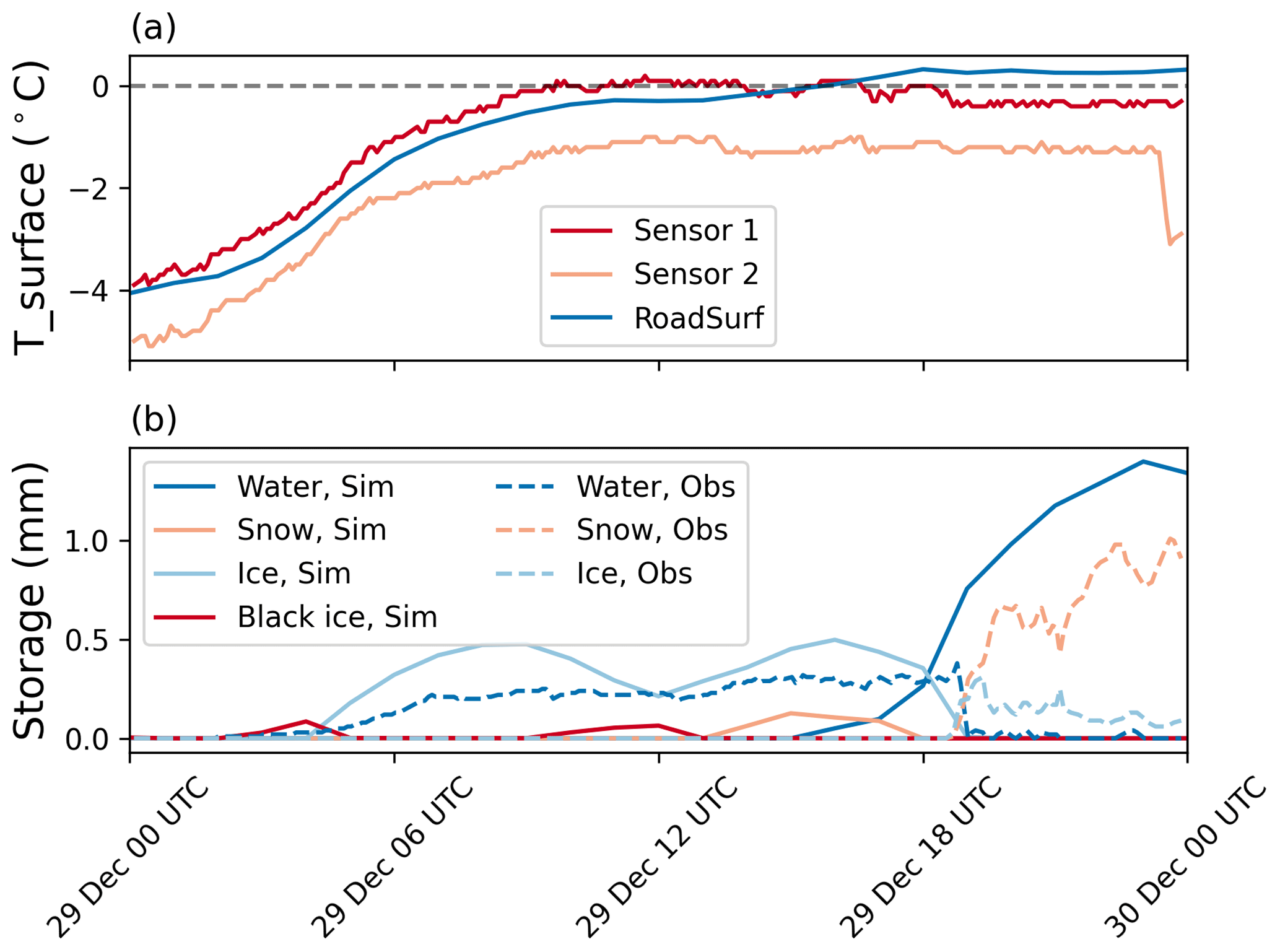
Figure 3 An example hindcast made with the RoadSurf library. The forecast data start time was 29th December 2022, 00:00 UTC, and the simulation point was the road weather station in Porvoo (60.38° N, 25.59° E). Panel (a) shows simulated (blue line) and observed road surface temperature (T_surface) with two different sensors (red line and peach-colored line). Panel (b) shows the observed (dashed lines) and simulated (continuous lines) amount of water (blue line), snow (peach-colored line), and ice (light-blue line) on the road as water equivalent millimeters. RoadSurf also simulates black ice, which is shown by the red line.

4.4 Example hindcast

Figure 3 shows an example hindcast done with the RoadSurf library. The road weather station had two surface temperature sensors. Sensor 2 gives somewhat colder measurements than sensor 1. The reason for this can be that sensor 2 is installed on a colder location on the road or that one of the sensors is calibrated incorrectly. The simulated surface temperature fits the observed ones quite well but is somewhat too warm at the end of the simulation. During daytime the surface temperature measured by sensor 1 is close to zero, whereas the simulated surface temperature is slightly colder. The observations show that there is water on the road, whereas in the simulation the road is icier. This turns around in the evening, when the simulated surface temperature rises above 0 °C but the measured surface temperature by sensor 1 drops below zero. According to the observations the road gets snowy and icy, but in the simulation the ice melts. This example shows that just a slight difference in predicted and observed surface temperature can lead to great differences in the predicted and observed road condition.

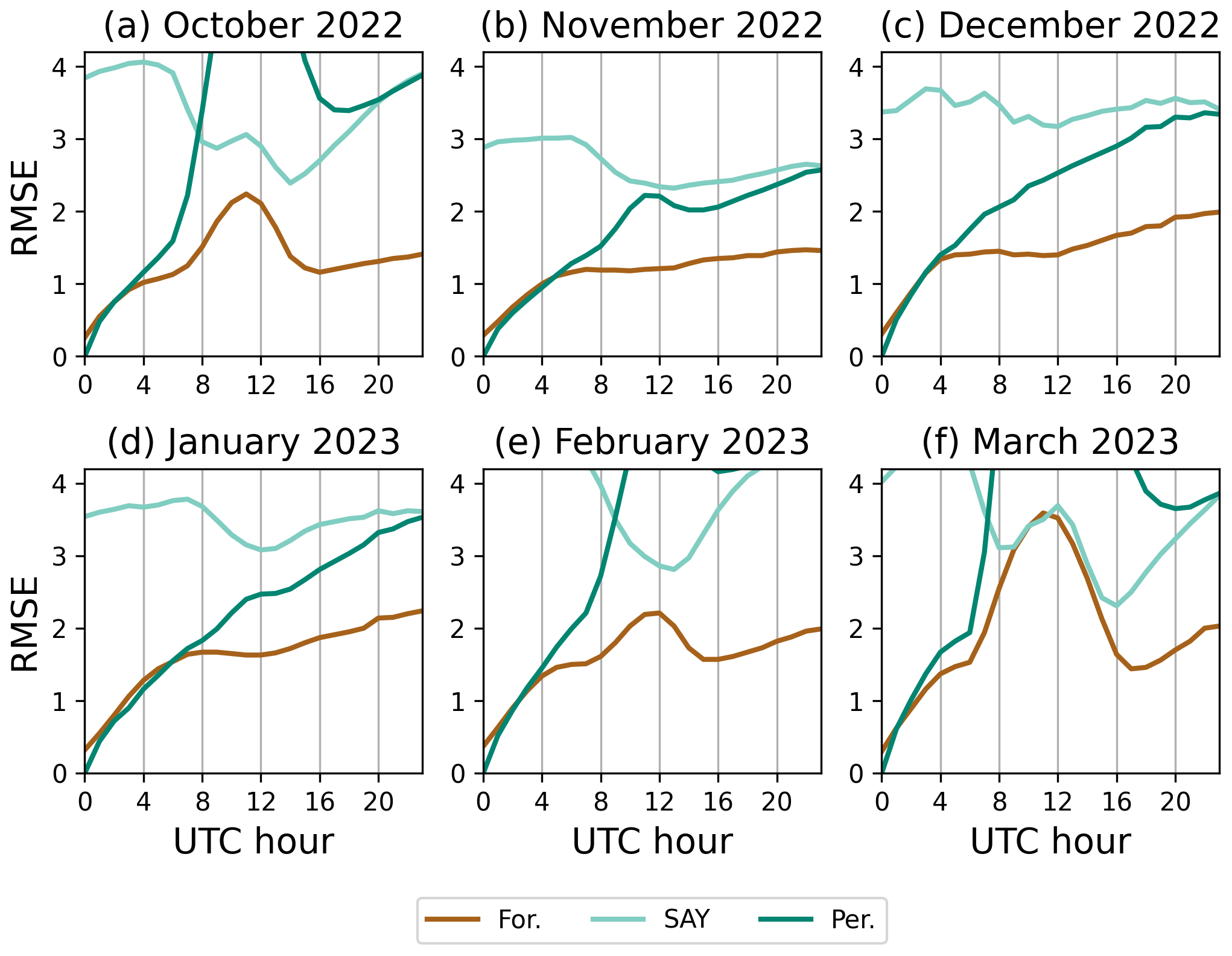
Figure 4 RMSE of the road surface temperature forecasts and of the dummy forecasts as a function of UTC time calculated over all road weather stations in Finland. Each panel shows results for 1 month from October 2022 to March 2023. The forecast start time was 00:00 UTC each day. Brown lines show the bias of the RoadSurf forecast, light-turquoise lines of the dummy forecast forecasting the same surface temperature as the day before at the same time, and the turquoise lines of the dummy forecast forecasting the same surface temperature as at the forecast start time.

Figure 5 Same as Fig. 4 but for bias.

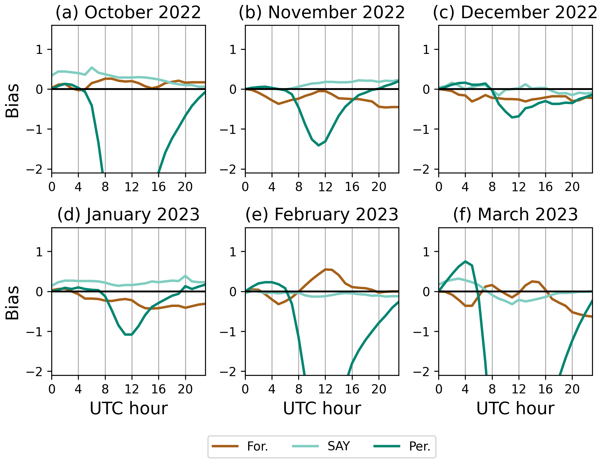
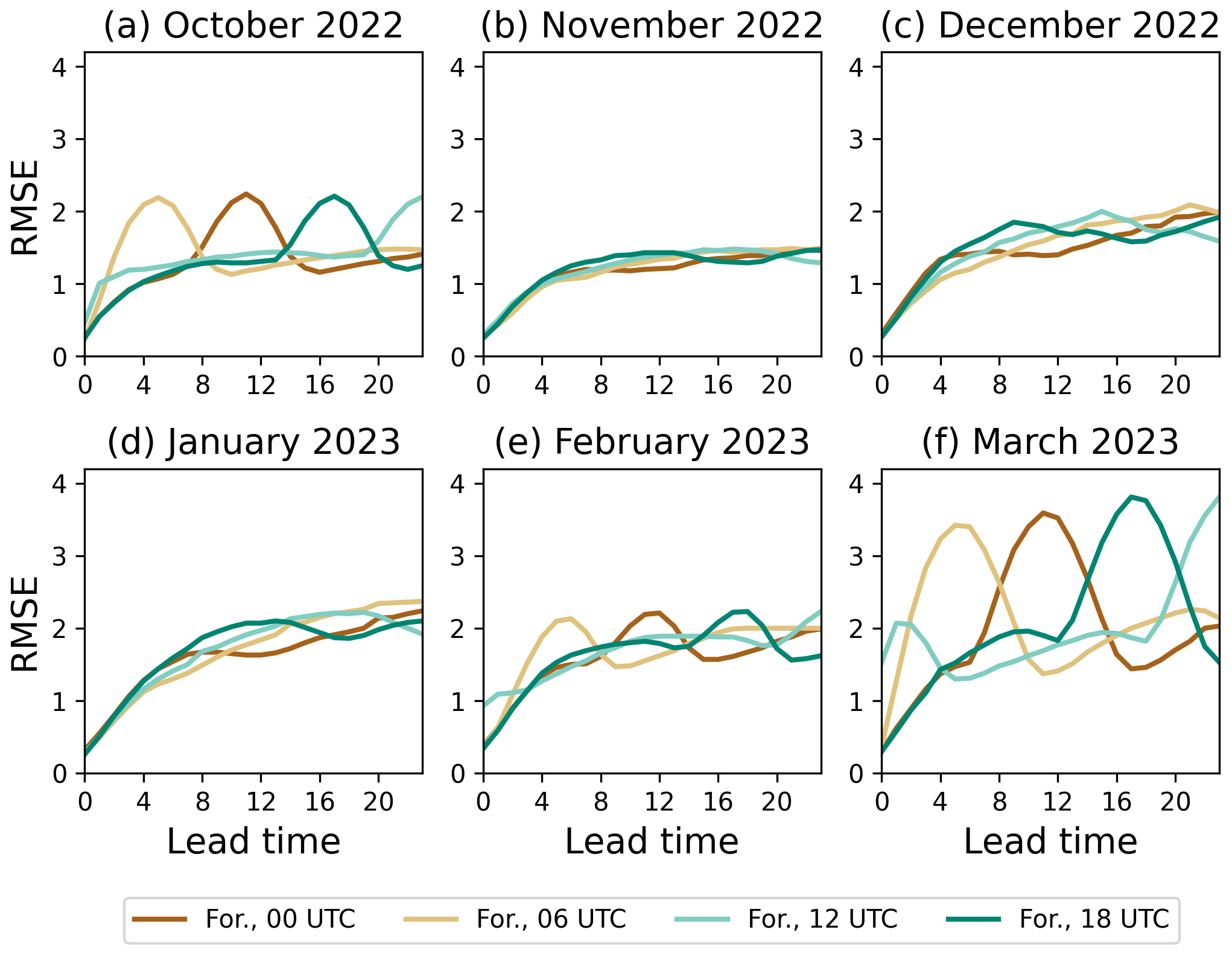
Figure 6 RMSE of the road surface temperature forecasts as a function of forecast lead time calculated over all road weather stations in Finland. Each panel shows results for 1 month from October 2022 to March 2023. Brown lines show the bias of the RoadSurf forecast started at 00:00 UTC, light-brown lines of the forecasts started at 06:00 UTC, light-turquoise lines for the forecast started at 12:00 UTC, and turquoise lines for forecast started at 18:00 UTC.

Figure 7 Same as Fig. 6 but for bias.

5 RoadSurf evaluation

Simulations done with the RoadSurf library were evaluated against road surface temperature observations. Figures 4 and 5 show the root mean square error (RMSE) and bias (forecast − observation) for the 00:00 UTC started hindcasts for each month. These hindcasts are henceforth referred to as forecasts for simplicity. The figures also show results for two “dummy” forecasts as a reference. The first dummy forecast always forecasts the same surface temperature as observed on the previous day at the same time. From now on it will be referred to as SAY (same as yesterday). The second dummy forecast is a persistence forecast that always forecasts the same road surface temperature as the observation at the forecast start time. The RMSE of the RoadSurf forecast and the persistence forecast are quite similar in the first hours of the forecast. The persistence forecast gives slightly better results at first, but the error quickly increases to be much greater than for the RoadSurf forecast. The persistence forecast works better in wintertime than in autumn and spring because the daily surface temperature variation is smaller. The SAY forecast gives considerably greater RMSE error than the RoadSurf forecast for all months and lead times except during daytime in March, where they are quite similar. The RoadSurf library has difficulties forecasting maximum surface temperatures when the daily variation in surface temperature is large.

The bias of the RoadSurf forecast is generally quite small. From November to January the forecasts are a little too cold, but in October, February, and March there is some warm bias during daytime. The persistence forecast also has quite small bias during nighttime but has very negative values during daytime. The bias of the SAY forecast is also quite small. In October and in January it is generally a little positive, which indicates that there was a general decreasing trend in surface temperature during October and January.

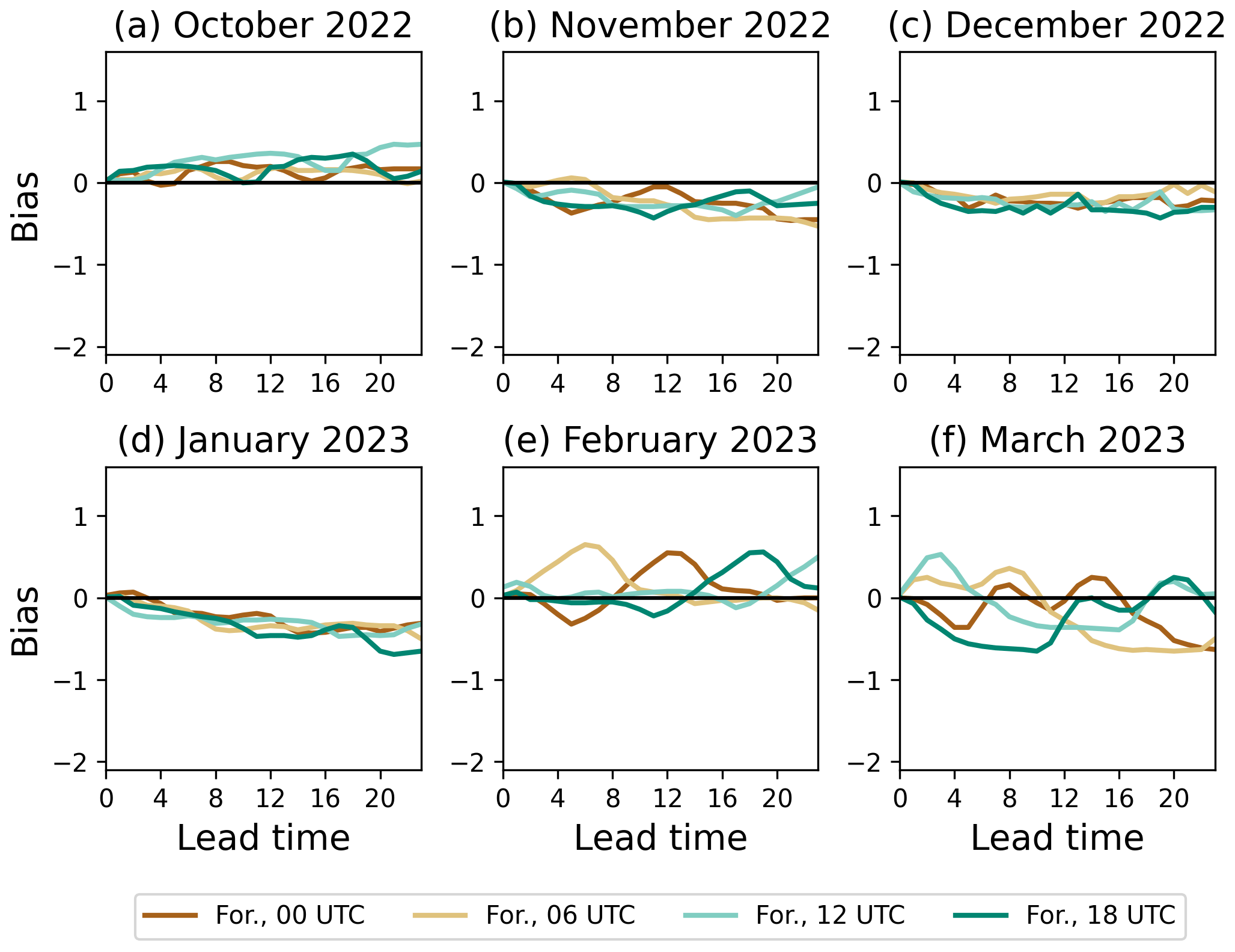
As the daily surface temperature variation is quite large in autumn and spring, the forecasts with different starting times were evaluated separately. Figures 7 and 6 show the bias and RMSE for the forecasts started at 00:00, 06:00, 12:00, and 18:00 UTC. Similarly to 00:00 UTC started forecasts, the forecasts with other start times have RMSE maxima during daytime in October, February, and March. During those months the 12:00 UTC started forecast has a little higher RMSE at the forecast start time. This is because the forecast starts around the time of the daily surface temperature maximum. From November to January the RMSE values are rather similar, but there is some daily variation as well. The 00:00, 06:00, and 18:00 UTC forecasts seem to have smaller RMSE values when the actual forecast time is around 12:00 UTC. During those months, the daily temperature variation caused by solar radiation is rather small. However, there still is about 1.5 °C difference between minimum and maximum hourly mean temperatures calculated over the month. It seems that the simulation forecasts the slightly warmer daytime temperatures better.

All forecasts with different starting times have small positive bias in October. During November, December, and January the bias is mostly negative. In February, all forecasts with different start times have some positive bias during daytime. There is also some positive bias in March during daytime, but the bias seems to have a local minima around 12:00 UTC. During nighttime in March all forecast start times have negative bias.

The evaluation results were calculated over all road weather stations in Finland, but naturally the results vary from station to station. The evaluation focused only on road surface temperature because the amounts of water, ice, and snow measured by the road weather station are not considered reliable enough for proper evaluation. It should be noted that the simulations are very sensitive to the input data. If the atmospheric forecast given as input to the simulation is of poor quality, then probably so is the road weather forecast. In this evaluation, the atmospheric forecast data were from the FMI operational weather forecast, which is the best data FMI has to offer. The newest operational forecast is available as open data in the FMI open-data service (https://en.ilmatieteenlaitos.fi/open-data, last access: 14 June 2024).

6 Conclusions

RoadSurf is a Fortran library that contains functions for predicting winter road conditions. The functions of the library can be used to set up the road weather forecasting system. The most important predicted variable is road surface temperature, which is simulated by calculating surface heat balance and temperature transfer in the ground. The library is also able to forecast the amounts of water, ice, snow, and black ice on the road. Each of these has their own storage in the model, and they are increased and decreased through various processes, including precipitation, traffic wear, freezing, and melting. The requirements to use the library, as well as the main physics and evaluation against observations, have been presented in this paper. The evaluation showed that the RoadSurf library is well suited for predicting road surface temperature. The persistence forecast gives comparable results during the first forecast hours, but after 4–6 h the simulations done with RoadSurf perform clearly better. The evaluation results were better for months when there is less daily surface temperature variation, as forecasting daytime maximum surface temperatures is challenging when the daily surface temperature variation is great.

Forecasts created by RoadSurf can assist in keeping roads safe for drivers wherever wintry road conditions occur. The library allows flexible implementation. Each user can create their own program utilizing the library functions, or they can just implement a few functions in their own road weather model. RoadSurf allows users to create their own input and output handling functions, which makes it easier to implement the library in existing systems. It is advised to run the model with historical data before operational use and adjust the model parameters to fit into local conditions. The model results should also be evaluated regularly against observations. RoadSurf provides an alternative to a broadly used METRo road weather model, giving institutes and companies more options when creating and developing their forecasting systems. A version of the RoadSurf model in Python language is also under development. It will allow easier implementation for users not proficient in Fortran language. However, it still needs more validation and documentation before it can be published.

Appendix A

All notations used in Sect. 3 are explained in Tables A1–A6 for easier reference.

Table A1 Variables describing energy fluxes.

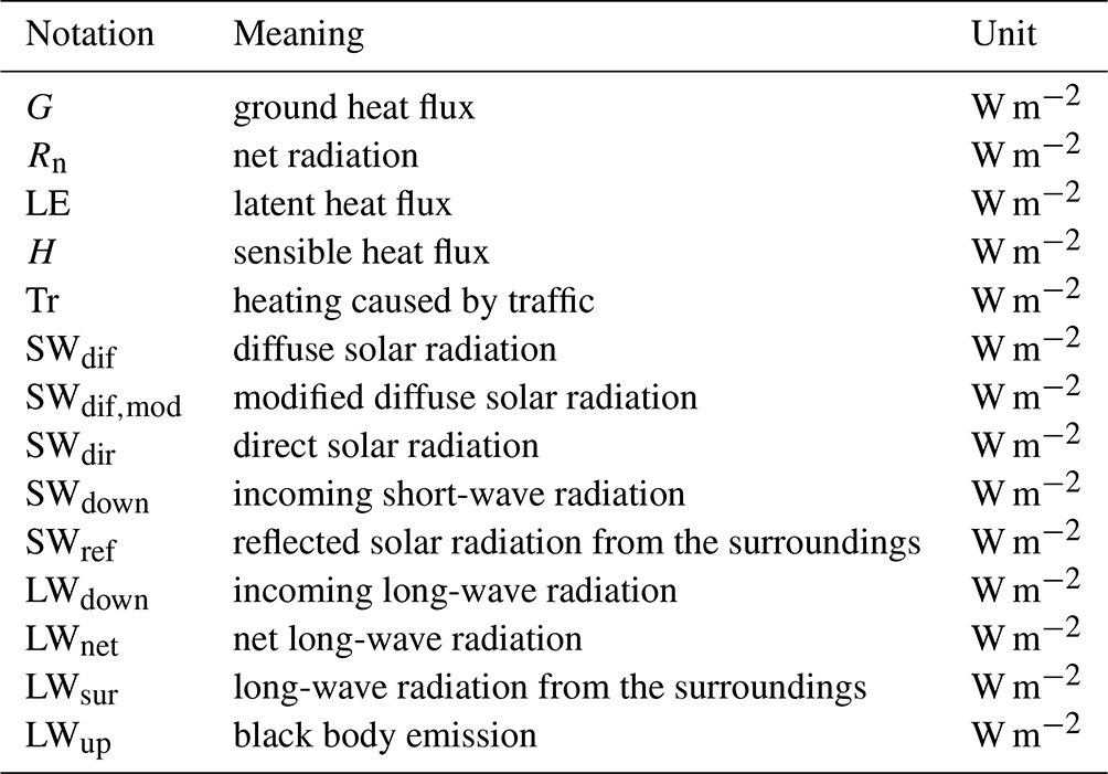
Table A2 Variables describing physical properties of the ground, air, and local environment.

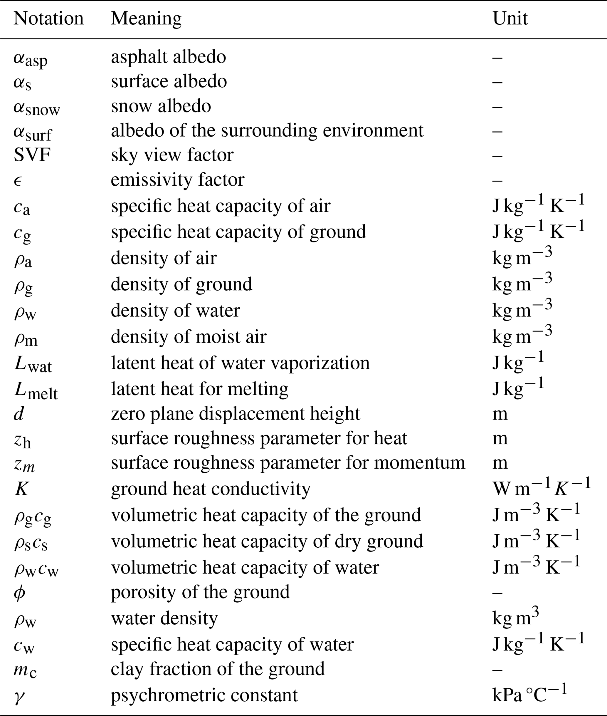
Table A3 Variables describing the current state of the ground, surface, and atmosphere.

Table A4 Physical constants.

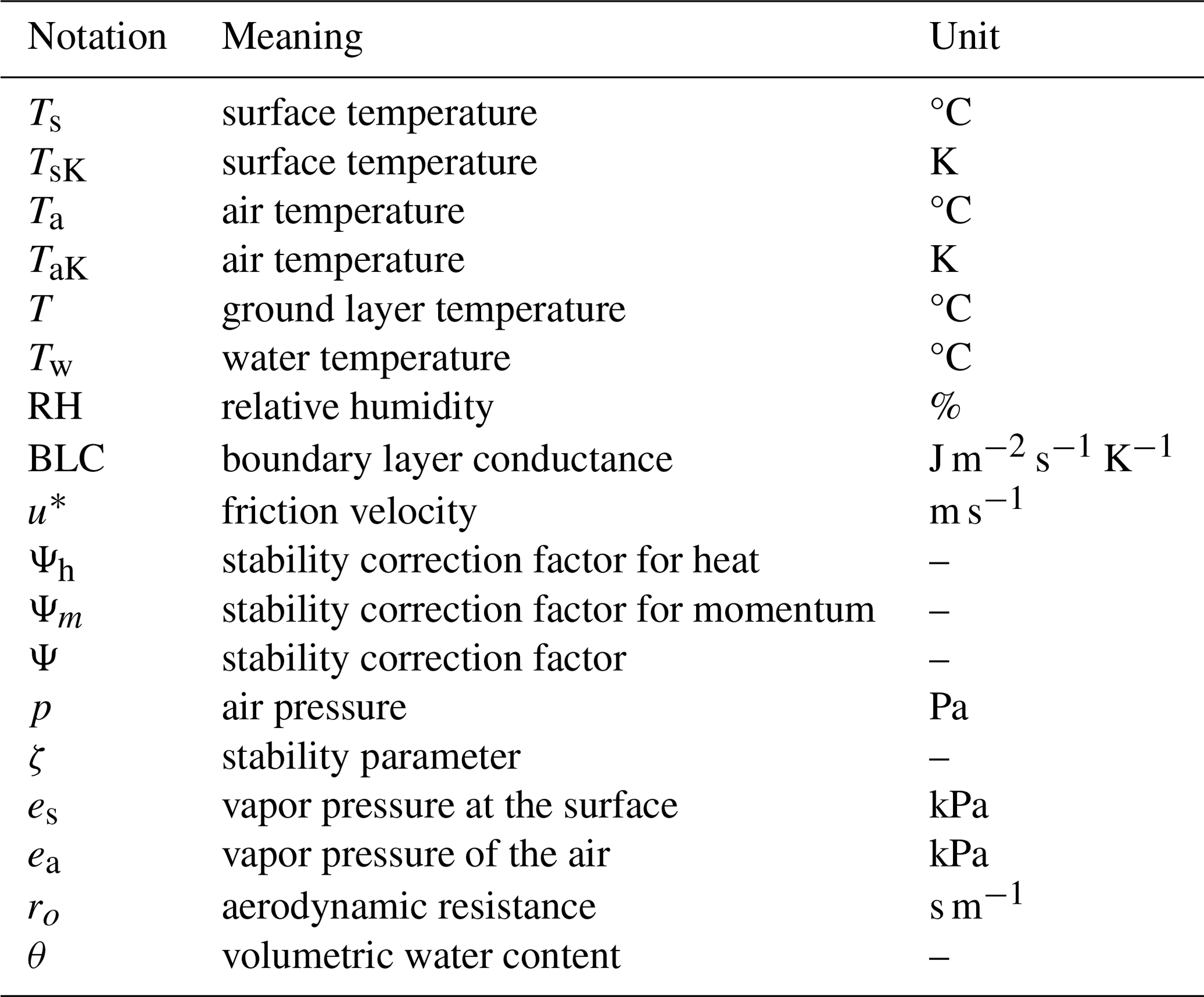
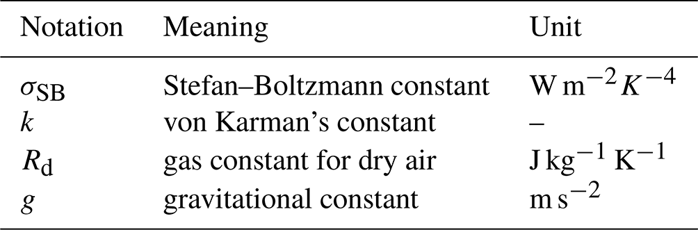
Table A5 Variables and parameters related to storage term calculation.

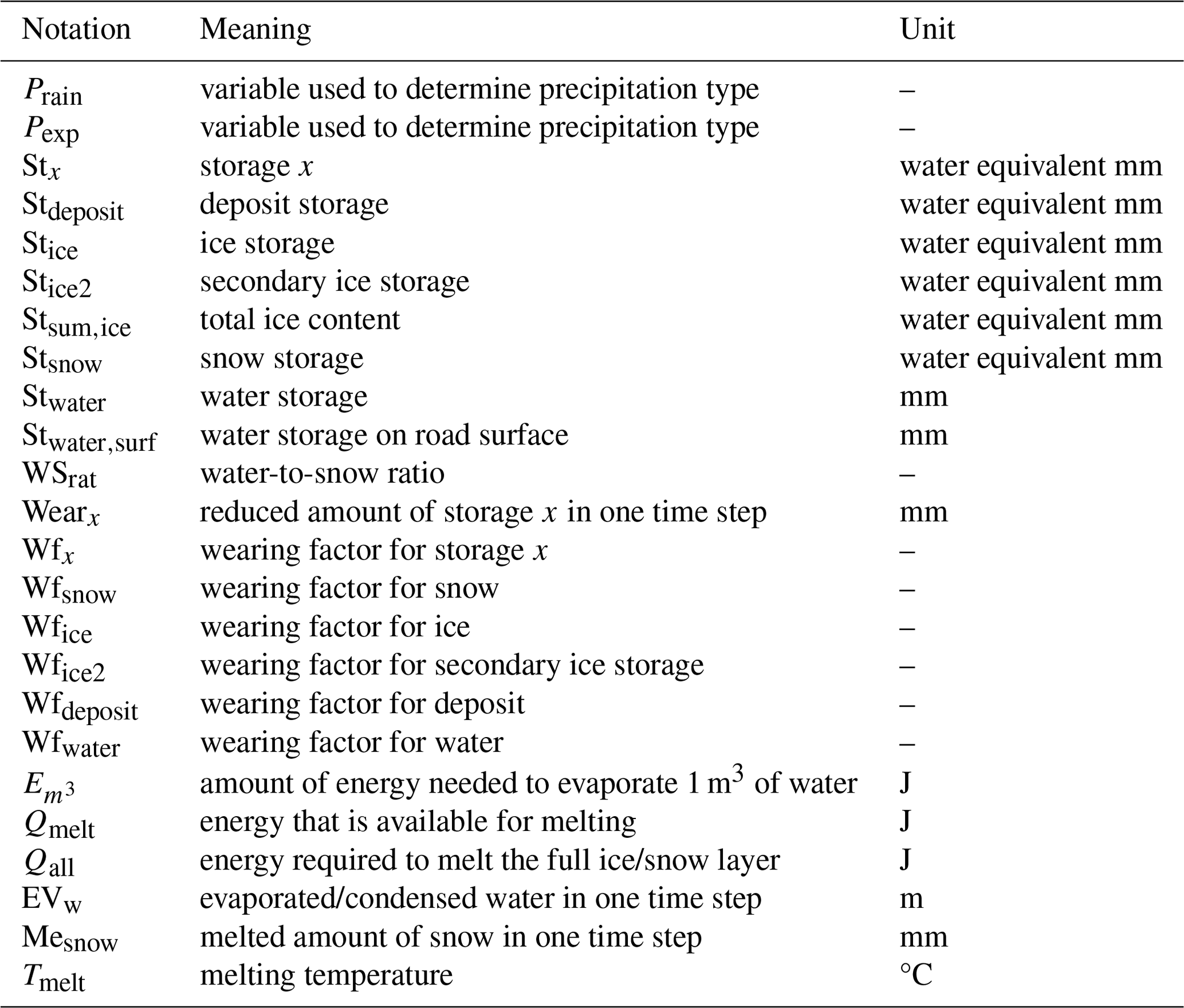
Table A6 Variables related to time and space and miscellaneous variables.