The ddeq Python library for point source quantification from remote sensing images (version 1.0)

Atmospheric emissions from anthropogenic hotspots, i.e., cities, power plants and industrial facilities, can be determined from remote sensing images obtained from airborne and space-based imaging spectrometers. In this paper, we present a Python library for data-driven emission quantification (ddeq) that implements various computationally light methods such as the Gaussian plume inversion, cross-sectional flux method, integrated mass enhancement method and divergence method. The library provides a shared interface for data input and output and tools for pre- and post-processing of data. The shared interface makes it possible to easily compare and benchmark the different methods. The paper describes the theoretical basis of the different emission quantification methods and their implementation in the ddeq library. The application of the methods is demonstrated using Jupyter notebooks included in the library, for example, for NO₂ images from the Sentinel-5P/TROPOMI satellite and for synthetic CO₂ and NO₂ images from the Copernicus CO₂ Monitoring (CO2M) satellite constellation. The library can be easily extended for new datasets and methods, providing a powerful community tool for users and developers interested in emission monitoring using remote sensing images.

1 Introduction

The majority of anthropogenic emissions of air pollutants and greenhouse gases is confined to localized sources such as cities, power plants and industrial facilities (e.g., Crippa et al., 2022). The emissions of these hotspots can be determined from the atmospheric plumes of trace gas column densities in remote sensing images. Trace gases of interest are nitrogen dioxide (NO_x = NO₂ + NO), carbon monoxide (CO), carbon dioxide (CO₂), methane (CH₄) and others. Numerous methods have been developed in recent years to quantify the emissions from remote sensing images by matching observations to simulated plumes (e.g., Bovensmann et al., 2010; Nassar et al., 2017; Broquet et al., 2018; Ye et al., 2020; Lei et al., 2021; Kaminski et al., 2022), applying the principle of mass conservation to individual or temporally averaged images (e.g., Beirle et al., 2011; de Foy et al., 2015; Varon et al., 2018; Reuter et al., 2019; Zheng et al., 2020; Kuhlmann et al., 2021; Leguijt et al., 2023), or using machine-learning models trained with synthetic observations (e.g., Jongaramrungruang et al., 2022; Joyce et al., 2023; Dumont Le Brazidec et al., 2024).

Remotely sensed trace gas images are available from space-based imaging spectrometers such as the TROPOspheric Monitoring Instrument (TROPOMI; Veefkind et al., 2012) and the Orbiting Carbon Observatory-3 (OCO-3; Eldering et al., 2019) and from high-resolution point source imagers such as GHGSat, several multispectral land imaging sensors (e.g., Sentinel-2) and the upcoming generation of missions in polar and geostationary orbits (i.e., Copernicus CO₂ Monitoring, CO2M; Geostationary Environment Monitoring Spectrometer, GEMS; The Global Observing SATellite for Greenhouse gases and Water cycle, GOSAT-GW; Sentinel-4 and Sentinel-5; Tropospheric Emissions: Monitoring of Pollution, TEMPO; and others). In addition, airborne imaging spectrometers can be used to map emission plumes at a high spatial resolution (e.g., Thorpe et al., 2017; Tack et al., 2019; Fujinawa et al., 2021). An example of the plumes that can be visible from a city or power plant is shown in Fig. 1. This example is from the synthetic SMARTCARB dataset (Kuhlmann et al., 2019) generated for the CO2M satellite constellation planned for launch in 2026 (ESA Earth and Mission Science Division, 2020).

Measurement-based emissions monitoring systems are currently being developed to support global efforts to reduce greenhouse gas emissions to achieve the goals of the Paris Agreement on climate change. One such system is the European CO₂ Monitoring and Verification Support (CO2MVS) capacity that will be implemented as part of the European Copernicus program (Janssens-Maenhout et al., 2020). A prototype system of the European CO2MVS capacity is currently developed as part of the CoCO2 project (https://coco2-project.eu/, last access: 24 May 2024). Since one goal of CO2MVS is the global monitoring of emission hotspots, several emission quantification methods were implemented and benchmarked in the CoCO2 project using synthetic CO2M CO₂ and NO₂ observations and Sentinel-5P/TROPOMI NO₂ observations (Hakkarainen et al., 2024; Santaren et al., 2024). As the new generation of satellites will provide a large number of hotspot images (e.g., Kuhlmann et al., 2021; Wang et al., 2020), it is foreseen that computationally lightweight methods will be needed to process such a large amount of data in the operational CO2MVS system. Such methods will have to make optimal use of the information contained in the images without requiring expensive plume simulations with a high-resolution atmospheric transport model.

This paper describes the Python library for data-driven emission quantification (ddeq; version 1.0), developed as part of the CoCO2 project as a shared library for the implementation of various lightweight approaches. Although the various methods differ in many aspects, they share many pre- and post-processing steps including data input and output. The common interface thus makes ddeq a powerful tool not only for comparing and benchmarking different methods, but also for implementing new approaches. The ddeq library was originally developed as part of the SMARTCARB project for detecting and quantifying CO₂ and NO_x emissions in synthetic CO₂ and NO₂ images of the CO2M mission (Kuhlmann et al., 2019, 2020a, 2021), but it has also been used for quantifying NO_x emissions with the airborne APEX imaging spectrometer (Kuhlmann et al., 2022). ddeq is designed for the lightweight emission quantification of hotspots from remotely sensed images. A similar community-driven library exists for regional and global emission estimation with atmospheric model runs through the Community Inversion Framework (CIF; Berchet et al., 2021). The ddeq version presented here does not include machine-learning models, which were also considered in the CoCO2 project (Dumont Le Brazidec et al., 2023, 2024). ddeq has been used in the CoCO2 project for benchmarking the different methods using synthetic CO2M observations (Santaren et al., 2024) and TROPOMI NO₂ observations (Hakkarainen et al., 2024).

The paper has two parts. In the first part, we describe the general principles of lightweight emission quantification and describe the different methods. In the second part, we describe the common framework and interfaces provided by ddeq and details of the implementation of the different methods. The application of the ddeq library to synthetic CO2M observations for estimating CO₂ and NO_x emissions and to TROPOMI observations for estimating NO_x emissions is showcased in several Jupyter notebooks available in the Supplement.

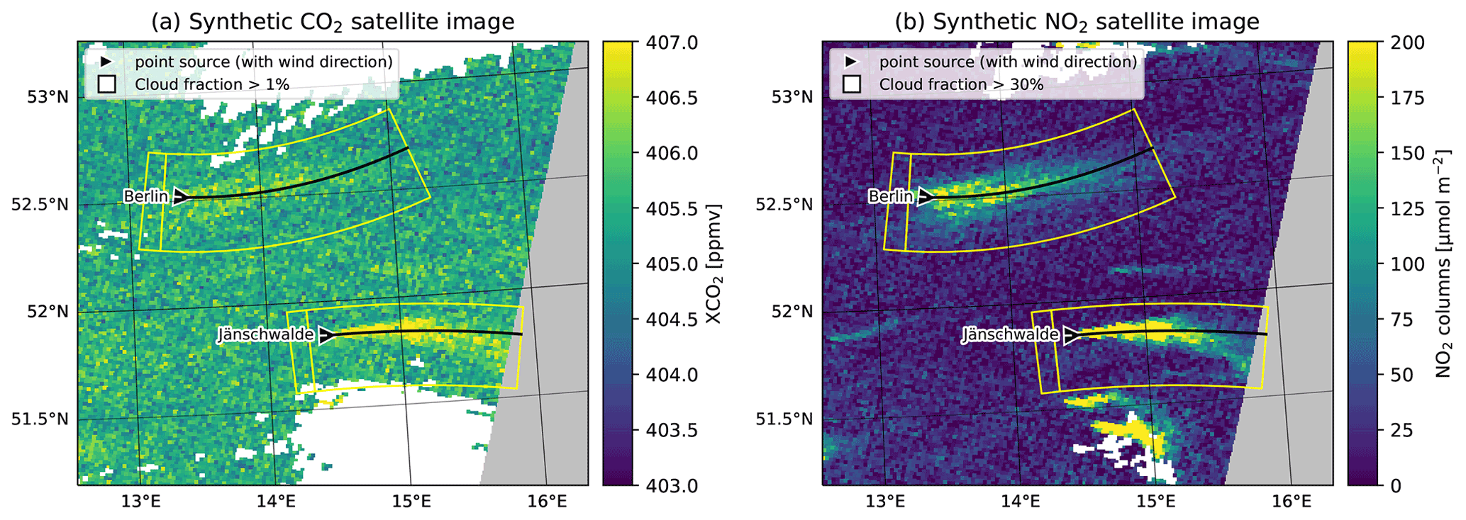
Figure 1 Example of synthetic CO2M (a) CO₂ and (b) NO₂ satellite images from the SMARTCARB dataset. The images show the emission plumes of the city of Berlin and the coal-fired power plant near Jänschwalde at a 2 km resolution. Pixels with cloud fractions larger than 1 % for CO₂ and 30 % for NO₂ are shown in white, and regions outside the satellite swath are shown in gray. The triangular marker indicates the wind direction at the source. The yellow polygons delineate the subregions containing the plumes. The smaller polygons show the regions upstream of the source.

2 Theoretical basis

Two families of lightweight approaches exists for emission quantification of hotspots. The first family quantifies emissions from “instantaneous plumes” obtained from single remote sensing images. The second family requires averaging over multiple images taken at different times before quantifying the emissions. The ddeq library currently implements four methods for emission estimation, partly in different flavors. The emission quantification methods are the (1) Gaussian plume inversion, (2) cross-sectional flux method, (3) integrated mass enhancement method and (4) divergence method. All methods can be applied to single images although the divergence method typically requires averaging over many images. In the following, the theoretical basis for plume detection, background estimation, effective wind speeds and the four quantification methods are summarized briefly. We also briefly cover the conversion of NO₂ to NO_x observations and the estimation of annual emissions from individual estimates.

Table 1 Symbols used in equations.

2.1 Identification of the plume region

A critical first step required by most methods is the identification of a subregion within the image (described by a polygon) where the emission quantification method is applied (see Fig. 1). The subregion contains the plume, i.e., the pixels where trace gas columns are enhanced due to emissions from the source of interest and a fraction of the background field. This first step not only identifies the plume location, but also assigns the source location and computes a local coordinate system defining along- and across-plume distances.

Broadly speaking, two different approaches to defining the subregion are available, and both have been implemented in ddeq. The first approach identifies the plumes inside the remote sensing images using an image segmentation algorithm. For example, if thresholding is used, pixels are assigned to the plume if their signal-to-noise ratio (SNR) exceeds a threshold, z_q:

$$\begin{array}{}\text{(1)}& \mathrm{SNR}={\displaystyle \frac{V-V_{\mathrm{bg}}}{{\mathit{\sigma }}_V}}\ge z_q,\end{array}$$

where V and V_bg are the total and background vertical column density and σ_V is the local noise in the image (Varon et al., 2018; Kuhlmann et al., 2019). The determination of the background, i.e., the vertical column density that would be expected without the presence of the source, is described in the next section. More complex segmentation algorithms apply feature detection using, for example, convolutional neural networks (Finch et al., 2022; Dumont Le Brazidec et al., 2023). The detected plumes can be assigned to one or more sources by checking their overlap with a known list of source locations, for example, from an emission inventory. The Boolean mask obtained from the image segmentation can be converted to the polygons shown in Fig. 1 by computing the bounding boxes in the local coordinate system.

The second approach determines the subregion based on the source location and the wind field available from, for example, a meteorological reanalysis product. This means that the remote sensing images are not used. In the simplest case, the wind vector is taken at the source location and the plume is assumed to be located downstream. It is then possible to draw a rectangular polygon with the along- and across-wind direction. The approach can be extended to simulate the plume location or an ensemble of plume locations with an atmospheric transport model, which can provide a better estimate of the plume location, especially further downstream of the source. However, this can get computationally quite expensive and does not qualify as a lightweight method anymore.

For each detected plume, a natural coordinate system can be established with the along-plume coordinate, x, and the across-plume coordinate, y. The coordinates can be computed as distance either along and perpendicular to the wind vector. For a curved plume, the coordinates can be computed as the arc length along and distance from a two-dimensional curve fitted to the detected plume (see Fig. 1 and Kuhlmann et al., 2020a for details).

2.2 Background estimation

To estimate the emission rate of a source, we are interested in the enhancement above the background:

$$\begin{array}{}\text{(2)}& V_{\mathrm{e}}(x,y)=V(x,y)-V_{\mathrm{bg}}(x,y).\end{array}$$

A common approach for estimating the background is applying a low-pass filter (e.g., a median filter) or a normalized convolution after masking enhancements, assuming a spatially smooth background field. Alternatively, the background can be estimated from the pixels upstream of the source. Another approach is explicitly fitting a background term in the emission quantification method, which is possible with Gaussian plume inversion and the cross-sectional flux method.

2.3 Effective wind speed

Wind speed and direction describe the transport of the trace gas in the atmosphere and are therefore important input parameters for all emission quantification methods. For methods that are applied to instantaneous images, the wind direction can be estimated from the plume direction. The wind speed needs to be taken from another source such as ECMWF's ERA5 reanalysis product (Hersbach et al., 2023).

To obtain an unbiased estimate of the emissions, it is necessary to calculate the effective wind speed that corresponds to the mean transport speed of the plume. The effective wind speed is the vertically averaged wind speed weighted by the vertical profile of the trace gas concentration. It can be calculated as

$$\begin{array}{}\text{(3)}& u(x,y)={\displaystyle \frac{{\int }_{\mathrm{0}}^{z_T}{\mathit{\rho }}_{\mathrm{e}}(x,y,z)u(x,y,z)\mathrm{d}z}{{\int }_{\mathrm{0}}^{z_T}{\mathit{\rho }}_{\mathrm{e}}(x,y,z)\mathrm{d}z}},\end{array}$$

where ${\mathit{\rho }}_{\mathrm{e}}(x,y,z)$ is the concentration of the trace gas enhancement, $u(x,y,z)$ is the along-plume wind speed and z_T is a height above the plume.

Since the vertical profile, ρ_e(z), is usually not known, a common approach to approximating the effective wind speed is by averaging the lowest layers of a reanalysis product (e.g., Fioletov et al., 2015, uses the mean of the three lowest ERA5 layers). Alternatively, plume rise calculations can be used to estimate the height and spread of the trace gas at the source location. The effective emission height can be significantly higher than the geometric height of a stack due to the momentum and buoyancy of the flue gas. Plume rise is generally influenced by stack geometry (height and diameter), flue gas properties (temperature, humidity and exit velocity) and meteorological conditions (wind speed and atmospheric stability) (Bieser et al., 2011; Brunner et al., 2019). In the case of a well-mixed atmospheric boundary layer, the exhaust plume becomes uniformly mixed throughout the depth of the boundary layer with increasing distance from the source. Therefore, a pressure-weighted mean wind speed in the boundary layer may be sufficient. This approach could also be viable for emissions from a city.

Lightweight approaches use a single value, such as the wind speed at the source location or averaged over the plume. It is important to note that the effective wind speed also has a temporal component, even in an instantaneous image, as the trace gas at the end of long plumes can be several hours old.

2.4 Emission quantification methods

Figure 2 illustrates the application of the Gaussian plume inversion, cross-sectional flux, integrated mass enhancement and divergence method. In each panel, the pseudo-color map shows the NO₂ column densities observed by an imaging spectrometer with a 5 km resolution for an emission plume of a source located at the origin. The plume was modeled with a Gaussian plume model with an emission rate of 1 kg s⁻¹ (≈ 32 kt NO₂ a⁻¹), a chemical lifetime of NO₂ of 6 h, and a wind speed of 5 m s⁻¹. The white crosses mark pixels where the NO₂ column is larger than 50 µmol m⁻². In the following, the theoretical basis for these methods is described for determining the emissions of a chemically inert gas (e.g., CO₂ and CH₄) and an exponentially decaying gas (e.g., NO₂). The conversion of NO₂ to NO_x is discussed in Sect. 2.5.

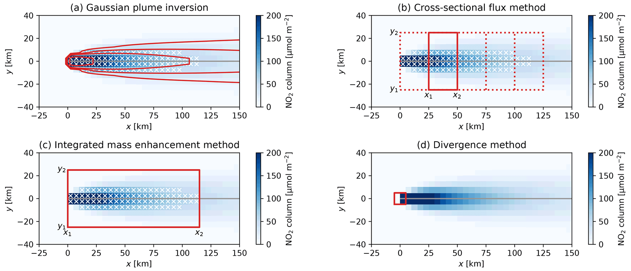
Figure 2 Sketch showing the application of the different lightweight methods to an emission plume. Each panel shows an NO₂ emission plume simulated by a Gaussian plume model (Q=1 kg s⁻¹; u=5 m s⁻¹), including exponential decay (τ=6 h).

2.4.1 Gaussian plume inversion

In this method, a vertically integrated Gaussian plume model, G, is fitted to the observed column densities, V (e.g., Bovensmann et al., 2010; Nassar et al., 2017). The Gaussian plume model can be written as

$$\begin{array}{}\text{(4)}& G(x,y)={\displaystyle \frac{QH\left(x\right)}{\sqrt{\mathrm{2}\mathit{\pi }}u\mathit{\sigma }\left(x\right)}}\exp \left(-{\displaystyle \frac{y^{\mathrm{2}}}{\mathrm{2}\mathit{\sigma }(x{)}^{\mathrm{2}}}}\right)+V_{\mathrm{bg}}(x,y),\end{array}$$

with emission rate Q, wind speed u and background column V_bg(x,y). H(x) is the Heaviside step function, and x and y are the along- and across-plume coordinates. The dispersion in the across-plume direction is modeled by the standard width

$$\begin{array}{}\text{(5)}& \mathit{\sigma }\left(x\right)=\sqrt{{\displaystyle \frac{\mathrm{2}K{x}^{\mathit{\kappa }}}{u}}},\end{array}$$

with the eddy diffusion coefficient, K (in m² s⁻¹). The additional exponent κ accounts for possible changes in the dispersion rate along the plume depending on meteorological conditions. This makes it possible to modify the standard expression using κ=1 with a power law of the form σ(x)=ax^b, which has also been used in the literature (e.g., Krings et al., 2013). An example of the Gaussian plume is shown by the contour lines in Fig. 2a.

A least-squares method can be used to obtain the optimal values for Q, K, V_bg and κ as well as their uncertainties by minimizing the following cost function:

$$\begin{array}{}\text{(6)}& J(Q,K,V_{\mathrm{bg}},\mathit{\kappa })={\left|\left|V_{i,j}-G(x_i,y_i)\right|\right|}_{\mathrm{2}}^{\mathrm{2}},\end{array}$$

where V_i,j is the observed column density for the pixel with center coordinates (x_i,y_i).

Equation (4) can be used to approximate the emission plumes for species with long lifetimes such CO₂, CO and CH₄. For species with short lifetimes, the Gaussian plume model needs to be multiplied with a decay term:

$$\begin{array}{}\text{(7)}& D(x,\mathit{\tau })=H\left(x\right)\exp \left(-{\displaystyle \frac{x}{u\mathit{\tau }}}\right),\end{array}$$

where the lifetime, τ, is an additional fitting parameter. In the case of NO₂, the lifetime is typically about 4 h.

The Gaussian plume model is valid for a point source, where the source area is smaller than the pixel size. For sources such as cities with dimensions larger than the pixel size, the flux slowly increases across the source area. An approach to accounting for this effect is to describe the emissions from the city by an emission map, p(x,y), and the change in flux in the along-plume direction as the convolution of a map and a decay term.

$$\begin{array}{}\text{(8)}& G_{\mathrm{a}}(x,y)=G(x,y)\underset{-\mathrm{\infty }}{\overset{+\mathrm{\infty }}{\int }}D(x^{\prime },\mathit{\tau })p(x-x^{\prime },y)\mathrm{d}{x}^{\prime }\end{array}$$

The emission map can take the form of a uniform surface within city boundaries or a two-dimensional Gaussian surface, p(x,y), with the form

$$\begin{array}{}\text{(9)}& \begin{array}{rl}p(x,y)& ={\displaystyle \frac{\mathrm{1}}{\mathrm{2}\mathit{\pi }{\mathit{\sigma }}_x{\mathit{\sigma }}_y\sqrt{\mathrm{1}-r^{\mathrm{2}}}}}\\ & \cdot \exp \left(-{\displaystyle \frac{(x-x_{\mathrm{0}}{)}^{\mathrm{2}}}{\mathrm{2}{\mathit{\sigma }}_x^{\mathrm{2}}(\mathrm{1}-r^{\mathrm{2}})}}-{\displaystyle \frac{(y-y_{\mathrm{0}}{)}^{\mathrm{2}}}{\mathrm{2}{\mathit{\sigma }}_y^{\mathrm{2}}(\mathrm{1}-r^{\mathrm{2}})}}\right.\\ & \left.+{\displaystyle \frac{r(x-x_{\mathrm{0}})(y-y_{\mathrm{0}})}{{\mathit{\sigma }}_x{\mathit{\sigma }}_y(\mathrm{1}-r^{\mathrm{2}})}}\right),\end{array}\end{array}$$

where (x₀,y₀) is the center position, σ_x and σ_y are the standard widths, and r is the correlation. These parameters can be included in the least-squares method as additional fitting parameters.

2.4.2 Cross-sectional flux method

The cross-sectional flux method applies mass conservation by computing the gas flux in the plume (F; in kg s⁻¹) downwind of the source from wind speed, u, and line density, q (e.g., Varon et al., 2018; Reuter et al., 2019; Kuhlmann et al., 2021), i.e., as follows:

$$\begin{array}{}\text{(10)}& F=u\cdot q.\end{array}$$

For a non-decaying gas, the flux is identical to the emission rate, Q, under the assumption of steady-state conditions and that turbulent mixing is negligible compared to advective transport in the along-plume direction. For a decaying gas, the flux decreases downstream of the source in the along-plume distance, x. In this case, the emission rate can be computed by compensating the flux for the along-plume decay:

$$\begin{array}{}\text{(11)}& Q={\displaystyle \frac{F\left(x\right)}{D(x,\mathit{\tau })}}.\end{array}$$

The line density is obtained by integrating the column enhancements in the across-plume direction from y₁ to y₂ at distance x:

$$\begin{array}{}\text{(12)}& q\left(x\right)=\underset{y_{\mathrm{1}}}{\overset{y_{\mathrm{2}}}{\int }}\left(V(x,y)-V_{\mathrm{bg}}\right)\mathrm{d}y,\end{array}$$

where the interval [y₁,y₂] needs to be sufficiently large to contain the full plume extent.

The line density can simply be obtained by integrating over the enhancements for all pixels within a rectangle (a polygon in the case of a curved plume) delimited by [x₁,x₂] and [y₁,y₂] (see Fig. 2b). However, a disadvantage of this approach is that the background needs to be estimated first and subtracted from the observed vertical columns. Another disadvantage is that missing pixels (e.g., due to clouds) need to be interpolated to obtain the correct line density. An often-used alternative approach is therefore fitting a Gaussian curve to all observations within the rectangle:

$$\begin{array}{}\text{(13)}& g\left(y\right)={\displaystyle \frac{q}{\sqrt{\mathrm{2}\mathit{\pi }}\mathit{\sigma }}}\exp \left(-{\displaystyle \frac{(y-\mathit{\mu }{)}^{\mathrm{2}}}{\mathrm{2}{\mathit{\sigma }}^{\mathrm{2}}}}\right)+my+b,\end{array}$$

with standard width σ and center position μ. The background is approximated here by a linear function with slope m and intercept b. The Gaussian curve has the advantage that it automatically interpolates missing values. Furthermore, assuming that different trace gases share the same distribution in the lateral direction, the method can be expanded to use the standard width and center position estimated for one trace gas directly when fitting the Gaussian function for another gas. This is particularly attractive for the combination of NO₂ and CO₂ observations from the future CO2M mission. Since NO₂ can be measured with higher precision than CO₂ with current remote sensing instruments, images of NO₂ can provide a much stronger constraint on the width and position of the plume compared to the much noisier images of CO₂ (e.g., Reuter et al., 2019).

To increase the accuracy of the estimate, fluxes can be computed for multiple polygons downstream of the source. For a non-decaying gas, the estimated fluxes can simply be averaged. For a decaying gas, however, the emission, Q, can be obtained by additionally fitting the lifetime, τ, to the estimated fluxes. For point sources, where the pixel size is larger than the source area, a step function is assumed in the decay term; i.e., the flux increases stepwise from zero to the emission rate, Q, at the source location:

$$\begin{array}{}\text{(14)}& F_p(x,\mathit{\tau })=Q\cdot D(x,\mathit{\tau }).\end{array}$$

For sources such as cities, it is necessary to account for the effect of the source area by describing the emissions from the city, for example, as a Gaussian curve and the change in flux in the along-plume direction as the convolution of a Gaussian curve and a decay term

$$\begin{array}{}\text{(15)}& F_a(x,\mathit{\tau },{\mathit{\mu }}_{\mathrm{a}},{\mathit{\sigma }}_{\mathrm{a}})=Q\underset{-\mathrm{\infty }}{\overset{+\mathrm{\infty }}{\int }}D(x^{\prime },\mathit{\tau })g(x-x^{\prime },{\mathit{\mu }}_{\mathrm{a}},{\mathit{\sigma }}_{\mathrm{a}})\mathrm{d}{x}^{\prime },\end{array}$$

where μ_a and σ_a are the location and standard width of the Gaussian curve describing the extent of the area source. This is identical to the exponential modified Gaussian method but applied to a single image (Beirle et al., 2011; de Foy et al., 2015).

2.4.3 Integrated mass enhancement

The integrated mass enhancement approach computes the emission rate, Q, from the integrated total mass enhancement, M, of the detectable plume, 𝒫_d, and a residence time, t (Frankenberg et al., 2016; Varon et al., 2018). The method can be derived by integrating the Gaussian plume model after subtracting the background (Eq. 4) over a large polygon up to distance x₂ (see Fig. 2c):

$$\begin{array}{}\text{(16)}& M=\underset{y_{\mathrm{1}}}{\overset{y_{\mathrm{2}}}{\int }}\underset{x_{\mathrm{1}}}{\overset{x_{\mathrm{2}}}{\int }}\left(G(x,y)-V_{\mathrm{bg}}(x,y)\right)\mathrm{d}x\mathrm{d}y.\end{array}$$

If the integration interval in the across-plume direction is sufficiently large to contain the full plume and $\mathrm{0}<x_{\mathrm{1}}<x_{\mathrm{2}}$, we obtain

$$\begin{array}{}\text{(17)}& M=\underset{x_{\mathrm{1}}}{\overset{x_{\mathrm{2}}}{\int }}{\displaystyle \frac{Q}{u}}\mathrm{d}x\end{array}$$

or

$$\begin{array}{}\text{(18)}& Q={\displaystyle \frac{u}{L}}M,\end{array}$$

where u is the effective wind speed and $L=x_{\mathrm{2}}-x_{\mathrm{1}}$ is the length of the detectable plume. Note that the derivation here is different from Varon et al. (2018), who only integrated over the detectable plume and computed L as the length scale defined as the square root of the plume area.

In practice, M can be computed as

$$\begin{array}{}\text{(19)}& M=\sum _{(i,j)\in {\mathcal{P}}_{\mathrm{a}}}(V_{i,j}-V_{\mathrm{bg}})\cdot A_{i,j},\end{array}$$

where A_i,j is the pixel area and 𝒫_a is the integration area obtained by sufficiently expanding the detected plume in the across-wind direction to also include pixels with enhancements below the detection limit.

To apply the integrated mass enhancement method to a decaying gas, the decay term needs to be included in the integral:

$$\begin{array}{}\text{(20)}& M=\underset{y_{\mathrm{1}}}{\overset{y_{\mathrm{2}}}{\int }}\underset{x_{\mathrm{1}}}{\overset{x_{\mathrm{2}}}{\int }}G(x,y)\cdot D\left(x\right)\mathrm{d}x\mathrm{d}y.\end{array}$$

As a result, the emission rate, Q, can be computed as

$$\begin{array}{}\text{(21)}& Q={\displaystyle \frac{\mathrm{1}}{c}}{\displaystyle \frac{u}{L}}M,\end{array}$$

where the correction factor, c, corrects for the gas decay in the along-plume direction:

$$\begin{array}{}\text{(22)}& c={\displaystyle \frac{u\mathit{\tau }}{L}}\left(\exp \left(-{\displaystyle \frac{x_{\mathrm{1}}}{u\mathit{\tau }}}\right)-\exp \left(-{\displaystyle \frac{x_{\mathrm{2}}}{u\mathit{\tau }}}\right)\right).\end{array}$$

2.4.4 Divergence method

The divergence method was introduced by Beirle et al. (2011, 2019) for estimating NO_x emissions from TROPOMI NO₂ satellite observations. In the CoCO2 project, the method was adapted to estimate CO₂ emissions (Hakkarainen et al., 2022). The method is generally applied to a sequence of satellite images rather than a single image.

The divergence method is based on the continuity equation (Jacob, 1999; Koene et al., 2024) at steady state. According to this, the divergence of the flux field, F, corresponds to the difference between emissions, E, and sinks, S:

$$\begin{array}{}\text{(23)}& \mathrm{\nabla }\cdot \mathit{F}=E-S.\end{array}$$

The flux, F, is defined as

$$\begin{array}{}\text{(24)}& \mathit{F}=\left(\begin{array}{c}{F}_x\\ F_y\end{array}\right)=\left(\begin{array}{c}V\cdot u\\ V\cdot v\end{array}\right),\end{array}$$

where V is the vertical column density and u and v are the eastward and northward components of the plume transport speed, respectively, which correspond to the horizontal wind components weighted by the vertical distribution of the plume concentrations (Koene et al., 2024).

The NO_x sink can be calculated from the NO₂ columns as $S=\frac{fV}{\mathit{\tau }}$, where τ is the NO_x lifetime and f is the constant NO_x-to-NO₂ ratio. Assumptions about the lifetime and NO_x-to-NO₂ ratio are discussed in the next section.

In the case of gases like CO₂ with lifetimes much longer than the characteristic timescales of a plume (i.e., much longer than a few hours), the sink term can be neglected. For long-lived gases, however, it is critical to first subtract the atmospheric background before computing the divergence since the flux is not linear with column V due to the vertical change in wind speed (e.g., Hakkarainen et al., 2016).

To obtain the hotspot emissions, Q, from the emission map ($E=S+\mathrm{\nabla }\cdot \mathit{F}$), a peak-fitting algorithm can be applied that fits a two-dimensional Gaussian surface with a background at each source location (x₀, y₀):

$$\begin{array}{}\text{(25)}& \begin{array}{rl}p(x,y)& ={\displaystyle \frac{Q}{\mathrm{2}\mathit{\pi }{\mathit{\sigma }}_x{\mathit{\sigma }}_y\sqrt{\mathrm{1}-r^{\mathrm{2}}}}}\cdot \\ & \exp \left(-{\displaystyle \frac{(x-x_{\mathrm{0}}{)}^{\mathrm{2}}}{\mathrm{2}{\mathit{\sigma }}_x^{\mathrm{2}}(\mathrm{1}-r^{\mathrm{2}})}}-{\displaystyle \frac{(y-y_{\mathrm{0}}{)}^{\mathrm{2}}}{\mathrm{2}{\mathit{\sigma }}_y^{\mathrm{2}}(\mathrm{1}-r^{\mathrm{2}})}}\right.\\ & \left.+{\displaystyle \frac{r(x-x_{\mathrm{0}})(y-y_{\mathrm{0}})}{{\mathit{\sigma }}_x{\mathit{\sigma }}_y(\mathrm{1}-r^{\mathrm{2}})}}\right)+p_{\mathrm{BG}},\end{array}\end{array}$$

with standard widths (σ_x, σ_y); correlation r; and a constant background in the divergence flux map, p_BG.

2.5 NO₂ to NO_x conversion

Many studies estimate emissions from NO₂ observations. However, NO₂ is emitted primarily as nitrogen monoxide (NO) and rapidly converted to NO₂ in the atmosphere. Emissions are therefore reported as nitrogen oxides (NO_x = NO₂ + NO) in NO₂ equivalents (kg NO₂ s⁻¹). Since imaging remote sensing instruments only measure NO₂ column densities, it is necessary to convert NO₂ to NO_x using a NO₂-to-NO_x ratio, f_V, representative of vertical columns

$$\begin{array}{}\text{(26)}& V_{{\mathrm{NO}}_x}(x,y)=f_V(x,y)\cdot V_{{\mathrm{NO}}_{\mathrm{2}}}(x,y)\end{array}$$

or a ratio, f_Q, for the estimated emissions

$$\begin{array}{}\text{(27)}& Q_{{\mathrm{NO}}_x}=f_Q\cdot Q_{{\mathrm{NO}}_{\mathrm{2}}}.\end{array}$$

If the conversion factor f_V is constant in space, f_V and f_Q are identical. However, the assumption of spatial (and temporal) homogeneity is generally not true for emission plumes, and more realistic models are currently being discussed (e.g., Hakkarainen et al., 2024; Meier et al., 2024).

2.6 Estimating annual emissions

Except for the divergence method, the methods described thus far allow us to quantify emissions from a single satellite image. To make statements about emissions over longer periods of time and to take advantage of the detection of a single source in multiple satellite images, one can compute a temporal average of the various computed emissions. Since the temporal coverage may be sparse and unevenly distributed over the year due to cloud cover and other factors, it may be useful to fill the gaps by making assumptions about the temporal variability. One possibility is to fit a seasonal cycle to the individual estimates using a low-order spline to approximate the time-varying emissions and to compute the annual mean emissions by integrating over the cycle (e.g., Kuhlmann et al., 2021). Extrapolating from a few single observations to an annual average is associated with significant uncertainties unless additional information on the true temporal variability is available (Hill and Nassar, 2019; Nassar et al., 2022). A further complication is the fact that satellite observations are often performed at the same time of day, providing almost no information on diurnal variability.

3 The ddeq Python library

In this paper, we describe version 1.0 of the library, which is provided in the Supplement. ddeq is an open-source library, whose latest release is available on the Python Package Index (PyPI; https://pypi.org/project/ddeq/). The issue tracker and the development version of the library are available on the project's website at https://gitlab.com/empa503/remote-sensing/ddeq (last access: 24 May 2024). How to install ddeq is described in Appendix A. The documentation of the library is available in the Supplement and also published on Read the Docs (https://ddeq.readthedocs.io/, last access: 24 May 2024).

3.1 General framework

The library consists of four main components as shown in Fig. 3. (1) The data input component provides functions for reading remote sensing images (e.g., S5P/TROPOMI observations and synthetic CO2M observations), hotspot locations (e.g., CoCO2 point source database; Guevara et al., 2024) and (effective) wind fields (e.g., ERA5 reanalysis product). (2) The second component provides pre-processing of the data, which includes plume detection, conversion between coordinate systems, unit conversions, and estimation of the background field. (3) To quantify the emissions, five modules are provided implementing a Gaussian plume inversion (hereafter abbreviated as GP in ddeq.gauss), general and light cross-sectional flux method (hereafter CSF in ddeq.csf and LCSF in ddeq.lcsf), integrated mass enhancement (hereafter IME in ddeq.ime), and divergence method (hereafter DIV in ddeq.div). (4) Finally, the library provides functions for post-processing, which includes methods for estimating annual emissions from individual estimates, for converting NO₂ to NO_x emissions, for visualizing the results and for writing data output in standardized NetCDF format.

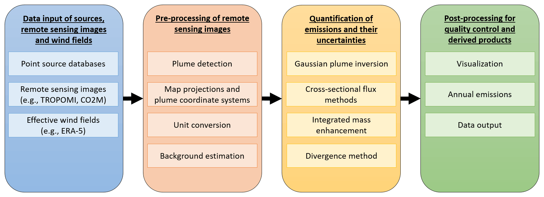
Figure 3 Data flow diagram illustrating the interactions between the different components in ddeq.

Listing 1 shows a simple code example demonstrating the individual steps required for estimating the CO₂ and NO_x emissions of the Jänschwalde power plant in Germany. The Jupyter notebook with the full example is part of the ddeq library (notebooks/tutorial-introduction-to-ddeq.ipynb). First, the data input step corresponds to reading the location of sources, synthetic CO2M data and ERA5 wind fields. ERA5 files were downloaded and prepared by the ddeq library (see Sect. 3.2). Second, a plume detection algorithm is used to locate the plume in the satellite image. A center curve is fitted to the data and natural coordinates are computed for the detected plume of each source. Third, the data are prepared for emission quantification by estimating and subtracting the background field and converting the CO₂ and NO₂ columns to kilograms per square meter. Fourth, CO₂ and NO_x emissions are estimated using the cross-sectional flux method as an example. The estimated NO₂ emissions are converted to NO_x using a conversion factor of 1.32 (in kg NO₂ s⁻¹). Finally, the results are saved as a NetCDF file and the data are visualized (see Fig. 4). In the following, the different components are described in more details. The implementation details are available in the documentation and the code itself in the Supplement.

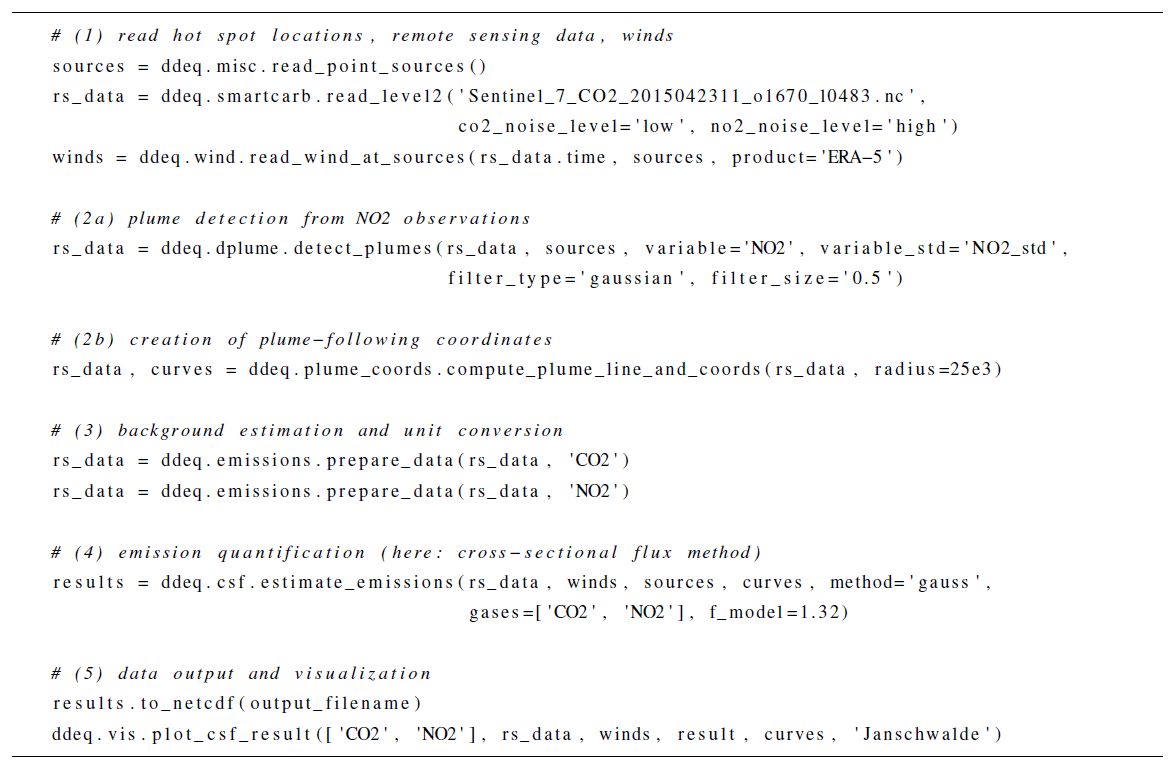
Listing 1 Example of ddeq code for applying the CSF method to estimate CO₂ and NO_x emissions of the Jänschwalde power plants in Germany. The full code is available in the library as a Jupyter notebook (notebooks/tutorial-introduction-to-ddeq.ipynb).

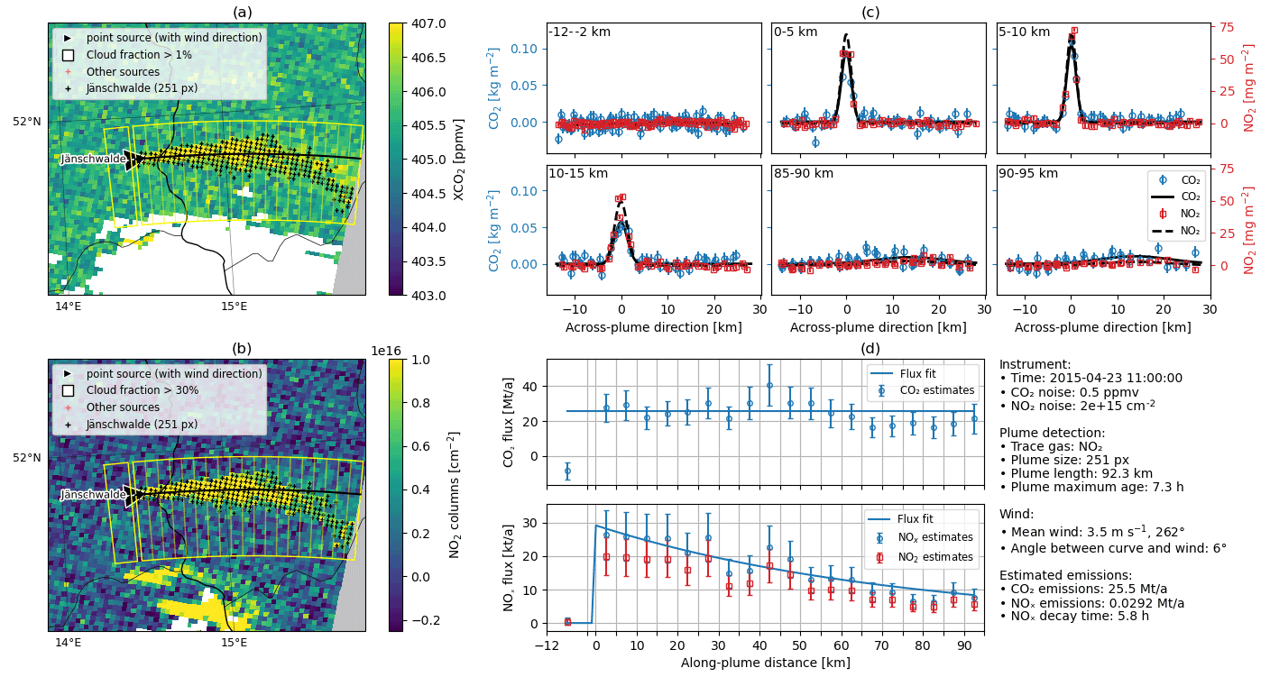
Figure 4 Plot created by the ddeq.vis.plot_csf_result command in the short example. Panels (a) and (b) show the CO₂ and NO₂ plumes from the Jänschwalde power plant in the synthetic CO2M images. Panel (c) shows the CO₂ and NO₂ columns in the across-plume direction for different along-plume distances with the two fitted Gaussian curves for computing the line densities. Panel (d) shows CO₂ and NO_x flux in the along-plume distance. The estimated CO₂ and NO_x emissions were 25.5 Mt a⁻¹ and 29.2 kt a⁻¹ for this example.

3.2 Data input

ddeq requires that the location of sources used is known prior to estimating the emissions. The location and type of sources is therefore an important input for plume detection and emission quantification. ddeq makes extensive use of the xarray package (Hoyer and Hamman, 2017) for data handling to combine arrays with attributes. Sources are read from a comma-separated values (CSV) file into xarray.Dataset, which contains the source names (source), longitudes (lon_o), latitudes (lat_o), labels for visualization (label) and source types (type, which is currently either city or power plant). ddeq maintains a small list of sources as a CSV file that primarily contains cities and power plants used in previous studies by the developers. User-defined files containing other sources can be prepared in the same format. The file can be read with the ddeq.misc.read_point_sources function. In addition, ddeq can read the comprehensive CoCO2 global emission point source database (Guevara et al., 2024) using ddeq.coco2.read_ps_catalogue. The catalogue is provided together with the library.

Remote sensing images are provided by airborne and space-based imaging spectrometers. ddeq handles images with xarray.Dataset with variables (i.e., rs_data in the example code), providing the trace gas columns and their uncertainties (e.g., CO2 and CO2_precision) that need to have a units attribute for automatic unit conversion and a noise_level attribute that is used as random uncertainty by the plume detection algorithm. In addition, the central longitude and latitude of the pixels need to be provided as lon and lat. If trace gases are provided as column-averaged mole fractions, surface pressure needs to be provided as psurf for unit conversion. Units are converted using the ucat Python library (https://pypi.org/project/ucat/, last access: 24 May 2024).

ddeq provides functions for automatically downloading and cropping TROPOMI NO₂ data for a given list of sources (ddeq.dowload_S5P). Furthermore, the library can read the synthetic CO2M and Sentinel-5 data from the SMARTCARB dataset (Kuhlmann et al., 2020b) and the simulations from the library of plumes generated in the CoCO2 project (Koene and Brunner, 2022). The synthetic datasets with known true emissions were used in the CoCO2 project for method development and benchmarking (Santaren et al., 2024).

The final important input for emission quantification are wind fields, from which a representative transport speed of the trace gas within the plume is computed. ddeq provides functions for reading and downloading ERA5 reanalysis fields as well as reading wind fields from the SMARTCARB project (ddeq.era5 and ddeq.wind). Wind speed and direction are provided either at the location of the source (ddeq.wind.read_at_sources) or as two-dimensional field that can also be spatially interpolated to the remote sensing image pixels, for example, for computing fluxes on Level-2 data (ddeq.read_field). Transport speeds can be computed by averaging the winds over a range of pressure levels, over the depth of the planet boundary layer or as weighted averages weighted by a vertical profile such as a typical emission profile of power plants (Brunner et al., 2019). The wind fields include the precision of the winds, currently hard-coded as 1 m s⁻¹, which is a rough estimate based on values used in previous studies (e.g., Varon et al., 2018; Reuter et al., 2019; Kuhlmann et al., 2021). Users are encouraged to replace the uncertainty with a value suitable for their application and can also use their own wind data from other data sources.

3.3 Pre-processing

Data pre-processing includes a plume detection algorithm, conversion between coordinate systems, unit conversions and estimation of the background field. Which pre-processing steps are required or optional depends on the individual method.

One main pre-processing step is an algorithm for identifying the (a priori) location of the emission plume in the remote sensing image. ddeq implements an image segmentation algorithm for plume detection that is used as a pre-processing step by the GP, CSF and IME methods. As an alternative, the LCSF method determines the (a priori) plume location from the source location and the wind vector, which is currently part of the method's implementation. The divergence method does not require information about plume locations.

The image segmentation algorithm is described in detail in Kuhlmann et al. (2019, 2021). In short, the algorithm generates a Boolean mask, which is true where column densities are significantly enhanced above the background using Eq. (1). The signal is computed as the difference between the local mean and the background field. The noise (σ_V) is computed from the random and systematic uncertainty in the vertical column densities and uncertainties in the background. The local mean is computed by applying a uniform or a Gaussian filter to the image. The background field is computed using a median filter with a kernel that is large enough to contain areas outside the plume. The threshold (z_q) is computed from the probability (q) that the local mean is larger than the background given the uncertainty σ_V based on a statistical z test. In the Boolean mask, neighboring pixels are connected to regions and regions overlapping with known sources are labeled as plumes. The ddeq.dplume.detected_plumes function is used for applying the algorithm to the remote sensing images.

To create the natural coordinate system and compute the plume length, a center curve can be fitted to the plume mask using the ddeq.plume_coords.compute_plume_line_and_coords function. The center curve is described by two parabolic polynomials from which the along-plume coordinate x is computed as the arc length from the source and the across-plume coordinate y is computed as the distance from the center curve (see Kuhlmann et al., 2020a for details). The plume length is the arc length from the source to the most distant detectable pixel. Prior to fitting the center curve, longitude and latitude are converted to eastings and northings using a Cartesian coordinate reference system object from the cartopy library (Met Office, 2010–2015). If pixel corners are provided by the input dataset, the function also computes the pixel size (in m²), which is required, for example, by the integrated mass enhancement method.

Finally, ddeq.emissions.prepare_data can be used to estimate the background field and convert all trace gas fields to mass columns (in kg m⁻²) using the ucat Python library (Kuhlmann, 2022). ddeq implements a function for estimating the background field from pixels surrounding a detected plume (ddeq.background.estimate). The function masks all pixels where the signal-to-noise ratio is larger than the threshold z_q (using the results from the plume detection algorithm) and applies a normalized convolution to estimate the background. Alternatively, the background can also be fitted directly by some emission quantification methods.

3.4 Emission quantification

3.4.1 Overview

Methods that are applied to single images all use the same order of parameters to estimate the emissions of sources:

results = ddeq.{method}.estimate_emissions(
    rs_data, winds, sources,
    [curves, gases, priors],
    variable='{gas}_minus_estimated_
     background_mass',
    [...]
)

where {method} can be gauss, lcsf, csf or ime for Gaussian plume inversion, light cross-sectional flux method, regular cross-sectional flux method and integrated mass enhancement method, respectively. Each method iterates over all sources provided by the sources dataset and estimates an emission if the source is inside the image. The method is applied to the variable in the remote sensing dataset (rs_data) given by the variable parameter (currently not implemented for LCSF and DIV). The default string is {gas}_minus_estimated_background_mass, which is the default variable name created by the pre-processing after subtracting the estimated background and converting to mass columns with units of kilogram per square meter. It is possible to provide a list of up to two gases for the CSF, GP and LCSF method (e.g, gases = ['NO2', 'CO2']). In this case, both gases are fitted either simultaneously (CSF) or after each other where the results from the first fit are used to constrain the second fit (GP and LCSF). The IME method can only be applied to a single gas. The {gas} placeholder in the variable parameter will be replaced with the names in gases.

The divergence method works on a series of remote sensing images and wind fields. The method therefore requires different inputs to read images and winds for a day on demand. The DIV method is called by

results = ddeq.div.estimate_emissions(
    datasets,
    wind_folder,
    sources, ...
)

where datasets is a class with a read_date method that returns a list of remote sensing images for a given date and wind_folder is the path to a folder containing wind fields, for example, from the ERA5 reanalysis or the COSMO atmospheric model, for each day. Examples for the dataset are the Level2Dataset class in the smartcarb module or the Level2TropomiDataset in the sats module.

All methods return a results dataset, which is an xarray.Dataset with at least the variables {gas}_estimated_emissions and {gas}_estimated_emissions_precision with dimension source that can be saved using the to_netcdf method. The CSF method stores the results datasets using the ddeq.misc.Result class, which inherits from dict to handle dimensions of different size between sources. It has the methods to_netcdf and from_file to write and read the results. The results are saved as NetCDF files using a group for each source. The implementation of the ddeq.misc.Result class is necessary as NetCDF groups are currently not supported by Xarray.

The total uncertainty in the estimated emissions depends on the uncertainty in the trace gas columns, wind speed and background field. Additionally, all methods rely on simplifications and assumptions (e.g., steady-state conditions), which may result in non-negligible uncertainties that are currently not accounted for in the ddeq library (see Santaren et al., 2024, for details). To determine the total uncertainty, users are therefore encouraged to include such uncertainties although they might be difficult to assess and vary from case to case.

3.4.2 Gaussian plume inversion (GP)

The Gaussian plume inversion method implemented in ddeq fits Eq. (4) to the detected plume. The fit parameters are Q, V_bg, K, κ and coefficients of the center line. The wind speed is taken from the winds dataset, which, when using ddeq.wind.read_at_sources, is the effective wind speed at the source.

The plume center curve is described by a second-order Bézier curve which has three control points (one is centered at the known plume source location, and the other two are fitted parameters for the Gaussian curve), initialized along the curve, as it is already obtained in pre-processing. The reason for using a Bézier curve is that it behaves smoothly with respect to small changes in the control points, which is required for stabilizing the least-squares fit. In the case of a decaying gas, it is possible to fit a decay time, τ, by setting fit_decay_times to true.

The inversion consists of three simple Levenberg–Marquardt least-squares fitting steps. In the first fit, only the center curve, Q and κ are optimized. In the second fit, K and τ are optimized, and in the third fit, Q is optimized again. The implementation of three fits decreases the computation time and avoids overfitting.

The initial (prior) parameters for Q and τ need to be provided as a dictionary for each source and trace gas:

priors = {
    source: {
      'CO2': {'Q': 1000.0, 'tau': 1e10},
      'NO2': {'Q': 1.0, 'tau': 4.0*3600},
    ...
}

where Q is the source strength (in kg s⁻¹) and tau is the decay time in seconds. Other parameters are set to typical values in the ddeq.gauss.generate_params function. If two gases are provided, the values fitted for the first gas are used as initial conditions for the second gas (except for Q, which is reinitialized to the prior emission rate for that source). To constrain the fit for the second gas, we only allow for a small amount of deviation around the previously obtained Gaussian plume parameters (see ddeq.gauss.gaussian_plume_estimates for details).

The precision or random uncertainty in the Gaussian plume estimate is computed as

$$\begin{array}{}\text{(28)}& {\mathit{\sigma }}_Q=\sqrt{{\mathit{\sigma }}_{Q,\mathrm{fit}}^{\mathrm{2}}+{\mathit{\sigma }}_u^{\mathrm{2}}{\left({\displaystyle \frac{Q_{\mathrm{fit}}}{u}}\right)}^{\mathrm{2}}},\end{array}$$

where σ_Q,fit is the estimated standard deviation of the fitted emission data and the second term accounts for the uncertainty in the wind speed as provided by the winds dataset (wind_speed_precision).

Estimates are rejected when no fit is found, when no standard deviation is estimated (i.e., if no good fit is possible), or when the emission rate is smaller than 0.1 times or larger than 1.9 times the prior expected emission rate (i.e., using Q±90 % uncertainty). These filters are currently fixed in the code. More flexible filters will be implemented in the future that are common to all methods.

3.4.3 Cross-sectional flux methods (CSF)

The CSF method is one of two different cross-sectional flux methods implemented in the library. The CSF method was originally developed as part of the SMARTCARB study (Kuhlmann et al., 2020a, 2021). It computes line densities in multiple polygons downstream of the source (see polygons in Fig. 4). Depending on the model parameter, line densities are obtained by either fitting a Gaussian curve (Eq. 13) using model="gauss" or integrating pixels inside the polygon using model="sub_areas". The latter method divides the sub-polygons in the across-plume direction, computes the mean for each sub-polygon, and then integrates the mean values for each sub-polygon. This is done to account for missing values in the image. For NO₂ observations, the f_model parameter can be provided to convert NO₂ to NO_x line densities.

The line densities are converted to fluxes using the provided wind speeds at the sources. Emissions are obtained by fitting Eqs. (14) or (15) to the fluxes. For a non-decaying gas, the decay function is replaced by a Heaviside step function, which is 0 upstream and 1 downstream of the source. The uncertainty in the cross-sectional flux method is computed by propagation of uncertainty from the single sounding precision that determines the uncertainty in each line density, which determines the uncertainty in the fitting parameters (Q and τ). Note that we assume that the wind speed uncertainty is independent of the number of pixels and the length of the plume.

To remove problematic cases, estimates are excluded if the angle between wind speed and center curve is larger than 45°, which often indicates erroneous plume detection. Estimates are also rejected if more than 5 pixels are detected upwind of the source.

3.4.4 Light cross-sectional flux method (LCSF)

The LCSF method is derived from the method originally developed by Zheng et al. (2020) to estimate the CO₂ emissions of Chinese cities and industrial areas from OCO-2 data. The method has then been adapted for routine and automatic estimation of isolated clusters of CO₂ emissions worldwide (Chevallier et al., 2020) and used to study the temporal variability in emissions using several years of OCO-2 and OCO-3 data (Chevallier et al., 2022).

Similarly to the CSF method, the LCSF method computes line densities by interpolating the pixels contained within polygons downstream of the source by a Gaussian function. The LCSF method uses the wind vector to construct a polygon that is 100 km wide in across-wind (perpendicular) direction and which extends downwind the source over a distance equal to the distance traveled by the wind in 1 h. A two-dimensional wind field read with ddeq.wind.read_field is used to determine the wind vector and for computing the wind speed used later for computing the flux. The fit_backgrounds parameter can be used to determine if a linearly changing background should be added to the Gaussian curve. Additional parameters are passed using a dictionary (lcs_params). For example, a NO₂ to NO_x conversion factor can be defined using the f_NOx_NO2 key (3.5 being the default).

The uncertainty in the estimates provided by the LCSF method is computed by propagation of the uncertainty in the amplitude of the fitted Gaussian function. Several quality checks remove potentially unrealistic estimates: the fitting window should contain enough data pixels (50 pixels being the default) and the selected enhancements should have sufficient amplitude (i.e., larger than the standard deviation of the values in the polygon), the uncertainty (1σ) of the fitted width of the Gaussian function should be larger than 1 km and smaller than 5 km, and the estimated emissions should be larger than min_est_emis (0.0 being the default) and smaller than max_est_emis (infinity being the default), which, when calling ddeq.lcsf.estimate_emissions, are provided either as input parameters or as prior values similar to the implementation for the Gaussian plume inversion (i.e., using 0.1 and 1.9 Q).

3.4.5 Integrated mass enhancement (IME)

To first identify the location of the plume, the IME method uses the plume detection algorithm with the same settings as for the CSF and GP method. IME also requires the computation of the background field, the center line and the along- and across-plume distance for each pixel. In the across-plume direction, the integration interval is obtained by either computing the convex hull of the detected plume or applying a binary dilation to the Boolean mask of detected pixels. Both computations are carried out as part of the pre-processing inside the ddeq.plume_coords.compute_plume_line_and_coords function. In along-plume direction, the integration interval is defined by the L_min and L_max parameters. The default values are L_min=0 (i.e., the source location) and L_max being set to the arc length of the most distant pixel in the integration area with 10 km subtracted from the value.

Missing values are interpolated using normalized convolution. The plume is discarded when more than 25 % of the pixels in the detected plume have been obtained through this gap filling. The effective wind speed is taken from the provided wind speeds at the source location. A decay time can be provided to compute the decay time correction term (Eq. 22).

The uncertainty in the emissions is calculated by propagation of uncertainty from the random uncertainty in the gas columns and the wind speed.

3.4.6 Divergence method (DIV)

In ddeq, the divergence method is applied to each source individually. The remote sensing images are provided as a dataset class as described above, where images are read for each date between start_date and end_date. To access the wind fields, the folder containing the wind files is provided along with a filename pattern (e.g., ERA5-gnfra- %Y %m %dt %H00.nc).

The divergence method is performed in two steps. In the first step, the average divergence, ∇⋅F, and sink, S, fields are calculated from the vertical column densities and wind fields. In the second step, the peak fitting is applied to derive the hotspot emissions.

In the first step, the trace gas fields can be denoised using a median filter, and depending on the choice of the user, either the local or the regional background is removed. Next, each pixel is associated with interpolated u and v wind components from the provided wind fields, and the vector field, F, is derived using second-order accurate central differences as implemented in numpy.gradient. All the data are gridded to a regular kilometer grid defined by the user by the input parameters lon_km, lat_km and grid_resol given in kilometers. The divergence of the vector field is calculated before averaging over all available images. The computation of the divergence before averaging is preferred for remote sensing images with data gaps, for example, due to clouds (Hakkarainen et al., 2022; Koene et al., 2024). For NO_x, the sink term is calculated from the averaged vertical column densities, assuming a lifetime of 4 h.

In the second step, the peak fitting is performed using a least-squares fit between the averaged emission field, $E=S+\mathrm{\nabla }\cdot \mathit{F}$, and the peak fitting function, Eq. (25). The optimization is first done using the Nelder–Mead method from the scipy library. The uncertainty in the estimated emissions is obtained from the mismatch between the emission field, E, and peak fitting function; i.e., we assume that the chi square of the fit is the number of degrees of freedom. ddeq also implements the adaptive Metropolis algorithm (Haario et al., 2001) for sampling the posterior distribution (assuming a non-informative prior) to obtain an optimized estimate of the fitting parameters and their uncertainty.

3.5 Post-processing

The post processing step provides functions for data visualization (ddeq.vis) and for estimating annual emissions from individual estimates (ddeq.timeseries). In addition, it is possible to apply scaling factors to estimated emissions to convert NO₂ to NO_x emissions.

To convert NO₂ to NO_x emissions, it is possible to scale all estimated NO₂ emissions in the results dataset, i.e., variables that start with NO2 and have units of kg s-1, to NO_x emissions using the scalar f. The function convert_NO2_ to_NOx_emissions(results, f=1.32) is implemented in the ddeq.emissions module. A more complex NO₂ to NO_x conversion will be developed in the future to account for non-constant conversion factors.

ddeq provides functions for fitting a seasonal cycle using a cubic C spline with periodic boundary conditions to a time series of estimated emissions (ddeq.timeseries). Annual emissions and their uncertainties are obtained by integrating the seasonal cycle, as shown in the following code:

 fit, model, _, _, _ = ddeq.timeseries.fit(
      times,
      estimates,
      estimates_precision
 )

  annual, annual_precision = model.integrate(
      fit['x'],
      fit['x_std']
 )

A detailed example is available as a Jupyter notebook (example_annual_emissions.ipynb).

Finally, ddeq provides functions for visualizing the remote sensing images, the plume detection, and the results of the emission quantification using ddeq.vis.plot_{method}_result (e.g., Fig. 4). The library includes several Jupyter notebooks, with demonstrations for the different methods.

4 Conclusions

There have been many studies quantifying the emissions of hotspots in remote sensing images in the past and we expect significantly more studies in the future with the new generation of imaging satellites. The ability to monitor emissions of air pollutants and greenhouse gases is an important capability of remote sensing instruments. As information on emissions from hotspots can be politically sensitive, it is essential that the emission estimates are reliable, i.e., that the methodology used can be verified, for which an open-source library will be an invaluable tool.

ddeq is a community library that is open to new users and developers. The Jupyter notebooks with tutorials and examples make it easy for new users to learn how to apply the library to different datasets. ddeq is hosted as an open-source project on GitLab, making it possible for users and developers to submit bug reports and feature request. Finally, developers can further expand existing methods in ddeq or implement new methods. ddeq makes it possible to compare these additions with existing methods in a reproducible way, for example, using the same input data, increasing the reliability of estimates of anthropogenic emissions of air pollutants and greenhouse gases.

The ddeq library provides a general framework where new methods and options can be easily implemented. It will be further developed in the future, for example, in the CO2MVS Research on Supplementary Observations (CORSO) project, where ddeq will be used for quantifying CO and NO_x emissions from Sentinel-5P/TROPOMI and other satellite instruments. Furthermore, ddeq will be used for quantifying CH₄ emissions from observations of the newest Airborne Visible/Infrared Imaging Spectrometer (AVIRIS-4) operated by a consortium of Swiss research institutes led by the University of Zurich (Green et al., 2022). Future updates will further harmonize the different implementations, allowing for more flexibility and even better comparability between the different methods. It is also planned for it to provide support for machine-learning models such as the plume segmentation algorithm developed by Dumont Le Brazidec et al. (2023).

One main goal of the CoCO2 project is the development of prototype systems for anthropogenic emission monitoring. The ddeq Python library for data-driven emission quantification presents such a prototype for emission monitoring of hotspots using lightweight approaches. It was developed and used in the CoCO2 project to benchmark different emission quantification methods with the aim to identify the most suitable and accurate approaches to be implemented in the prototype of the European CO₂ monitoring system (Hakkarainen et al., 2024; Santaren et al., 2024).

Appendix A: Installation and interactive computing environment

The latest version of the ddeq library can be installed using the Python package manager, pip:

    python -m pip install ddeq

The development version of ddeq can be cloned using

    git clone https://gitlab.com/empa503/
     remote-sensing/ddeq.git

and then installed using pip. For the development version, it is useful to install it as editable (-e option):

    pip install -e ddeq/

The version described in this paper is available in the Supplement. The version can be installed using conda and pip with the following steps:

    # create Python environment
    conda create -n ddeq-test python=3.9
    conda activate ddeq-test

    # install additional packages
    conda install jupyterlab
    conda install pycurl

    # unzip tar.gz file in the Supplement
      and install using pip
    tar -xzvf ddeq-1.0.tar.gz
    python -m pip install ddeq-1.0/

    # start JupyterLab
    jupyter lab --notebook-dir

The tutorial and examples are included in the notebooks folder.