An improved and extended parameterization of the CO₂ 15 µm cooling in the middle and upper atmosphere (CO2_cool_fort-1.0)

The radiative infrared cooling of CO₂ in the middle atmosphere, where it emits under non-local thermodynamic equilibrium (non-LTE) conditions, is a crucial contribution to the energy balance of this region and hence to establishing its thermal structure. The non-LTE computation is too CPU time-consuming to be fully incorporated into climate models, and hence it is parameterized. The most used parameterization of the CO₂ 15 µm cooling for Earth's middle and upper atmosphere was developed by Fomichev et al. (1998). The valid range of this parameterization with respect to CO₂ volume mixing ratios (VMRs) is, however, exceeded by the CO₂ of several scenarios considered in the Coupled Climate Model Intercomparison Projects, in particular the abrupt-4×CO₂ experiment. Therefore, an extension, as well as an update, of that parameterization is both needed and timely. In this work, we present an update of that parameterization that now covers CO₂ volume mixing ratios in the lower atmosphere from ∼0.5 to over 10 times the CO₂ pre-industrial value of 284 ppmv (i.e. 150 to 3000 ppmv). Furthermore, it is improved by using a more contemporary CO₂ line list and the collisional rates that affect the CO₂ cooling rates. Overall, its accuracy is improved when tested for the reference temperature profiles as well as for measured temperature fields covering all expected conditions (latitude and season) of the middle atmosphere. The errors obtained for the reference temperature profiles are below 0.5 K d⁻¹ for the present-day and lower CO₂ VMRs. Those errors increase to ∼1–2K d⁻¹ at altitudes between 110 and 120 km for CO₂ concentrations of 2 to 3 times the pre-industrial values. For very high CO₂ concentrations (4 to 10 times the pre-industrial abundances), those errors are below ∼1 K d⁻¹ for most regions and conditions, except at 107–135 km, where the parameterization overestimates them by ∼1.2 %. These errors are comparable to the deviation of the non-LTE cooling rates with respect to LTE at about 70 km and below, but they are negligible (several times smaller) above that altitude. When applied to a large dataset of global (pole to pole and four seasons) temperature profiles measured by MIPAS (Michelson Interferometer for Passive Atmospheric Spectroscopy) (middle- and upper-atmosphere mode), the errors of the parameterization for the mean cooling rate (bias) are generally below 0.5 K d⁻¹, except between $\mathrm{5}\times {\mathrm{10}}^{-\mathrm{3}}$ and $\mathrm{3}\times {\mathrm{10}}^{-\mathrm{4}}$ hPa (∼85–98 km), where they can reach biases of 1–2 K d⁻¹. For single-temperature profiles, the cooling rate error (estimated by the root mean square – rms – of a statistically significant sample) is about 1–2 K d⁻¹ below $\mathrm{5}\times {\mathrm{10}}^{-\mathrm{3}}$ hPa (∼85 km) and above $\mathrm{2}\times {\mathrm{10}}^{-\mathrm{4}}$ hPa (∼102 km). In the intermediate region, however, it is between 2 and 7 K d⁻¹. For elevated stratopause events, the parameterization underestimates the mean cooling rates by 3–7 K d⁻¹ (∼10 %) at altitudes of 85–95 km and the individual cooling rates show a significant rms (5–15 K d⁻¹). Further, we have also tested the parameterization for the temperature obtained by a high-resolution version of the Whole Atmosphere Community Climate Model (WACCM-X), which shows a large temperature variability and wave structure in the middle atmosphere. In this case, the mean (bias) error of the parameterization is very small, smaller than 0.5 K d⁻¹ for most atmospheric layers, reaching only maximum values of 2 K d⁻¹ near $\mathrm{5}\times {\mathrm{10}}^{-\mathrm{4}}$ hPa (∼ 96 km). The rms has values of 1–2 K d⁻¹ (∼20 %) below $\sim \mathrm{2}\times {\mathrm{10}}^{-\mathrm{2}}$ hPa (∼80 km) and values smaller than 4 K d⁻¹ (∼2 %) above 10⁻⁴ hPa (∼105 km). In the intermediate region between $\sim \mathrm{5}\times {\mathrm{10}}^{-\mathrm{3}}$ and $\sim \mathrm{2}\times {\mathrm{10}}^{-\mathrm{4}}$ hPa (85–102 km), the rms is in the range of 5–12 K d⁻¹. While these values are significant in percentage at $\sim \mathrm{5}\times {\mathrm{10}}^{-\mathrm{3}}$–$\mathrm{5}\times {\mathrm{10}}^{-\mathrm{4}}$ hPa, they are very small above $\sim \mathrm{5}\times {\mathrm{10}}^{-\mathrm{4}}$ hPa (96 km). The routine is very fast, taking (1.5–7.5) $\times {\mathrm{10}}^{-\mathrm{5}}$ s, depending on the extension of the atmospheric profile, the processor and the Fortran compiler.

1 Introduction

Carbon dioxide is the major infrared cooler of the atmosphere from the lower stratosphere up to the lower thermosphere, where emission by nitric oxide becomes important (López-Puertas and Taylor, 2001). However, the CO₂ infrared emissions in the ν₂ bands near 15 µm that are responsible for the cooling are in non-local thermodynamic equilibrium (non-LTE) above around 70 km (see e.g. López-Puertas and Taylor, 2001). Thus, in addition to the difficulty of computing the cooling rates in LTE, which requires the solution of the radiative transfer equation (RTE), i.e. a non-local problem, we have to calculate the non-LTE populations of the emitting levels. Thus, the calculation of the non-LTE cooling rates requires the solution of the statistical equilibrium equations for all energy levels producing a significant emission and the corresponding RTE equations for all bands originating from them (see e.g. Chap. 3 in López-Puertas and Taylor, 2001). Therefore, the exact calculation of non-LTE cooling rates in general circulation models (GCMs) or climate models that extend in height above the stratopause is virtually impractical, and hence efficient parameterizations of the CO₂ infrared cooling have been developed for implementation in such models.

The most used parameterization of the CO₂ 15 µm cooling for Earth's middle and upper atmosphere was developed by Fomichev et al. (1998). That parameterization is applicable for a limited range of CO₂ abundances, up to double the pre-industrial CO₂ concentration. Nowadays, however, with the rapid increase in the CO₂ concentration in the atmosphere and its expected increase in the coming decades, climate model projections are being carried out in much higher CO₂ scenarios that even quadruple the pre-industrial CO₂ abundance (van Vuuren et al., 2011; O'Neill et al., 2016). For example, such scenarios are considered in the Coupled Climate Model Intercomparison Projects. Therefore, parameterizations coping with such large CO₂ concentrations are highly in demand, and that is precisely the purpose of our work. In addition to that of Fomichev et al. (1998), other parameterizations of the CO₂ 15 µm cooling rates have been developed in the past. In the case of Earth's atmosphere, it worth mentioning the comprehensive review of the early works reported by Fomichev et al. (1998), the summary presented in Sect. 5.8 of López-Puertas and Taylor (2001) and the more recent work of Feofilov and Kutepov (2012). Further, just before this work was submitted, a new parameterization was developed that uses the accelerated lambda iteration and opacity distribution function techniques (Kutepov and Feofilov, 2023). For the Mars and Venus atmospheres, where CO₂ is the most abundant species, the problem has been tackled in several studies, e.g. López-Valverde et al. (1998), Hartogh et al. (2005), López-Valverde et al. (2008) and Gilli et al. (2017, 2021). In our case, we have the option of developing a completely new parameterization to adapt other CO₂ parameterizations (like those cited above) or to extend and improve the parameterization of Fomichev et al. (1998). Attending mainly to practical reasons of promptness, we opted for the latter.

The paper is structured as follows. A very basic description of the parameterization is presented in Sect. 2. Section 3 describes the input atmospheric parameters used in the parameterization and required for calculating the reference cooling rates. In Sect. 4 we describe the calculations of the reference LTE and non-LTE cooling rates. A detailed description of the parameterization is presented in Sect. 5. The testing and accuracy of the parameterization against (i) the reference cooling rates, (ii) the measured temperature fields of the middle atmosphere of MIPAS (Michelson Interferometer for Passive Atmospheric Spectroscopy) and (iii) the temperature profiles obtained by a high-resolution version of the Whole Atmosphere Community Climate Model (WACCM-X) are discussed in Sects. 6, 7 and 8, respectively. The previous cooling rate parameterization was commonly used together with a parameterization of the CO₂ near-infrared heating rates (Ogibalov and Fomichev, 2003) in GCMs. As we have extended the former to higher CO₂ volume mixing ratios (VMRs) and we do not plan to extend the latter to higher CO₂ VMRs in the near future, we assess in Sect. 9 the validity of the current near-infrared heating parameterization for high CO₂ VMRs. In Sect. 10, we summarize the main conclusions of the study.

2 Framework of the parameterization

As discussed above, this parameterization is essentially based on that of Fomichev et al. (1998). To compute the CO₂ cooling rate, the atmosphere is divided into five regions: one LTE and four different non-LTE regions. The method and approximations for computing the cooling rates in those regions are described in detail in Sect. 5. The new parameterization has a finer grid and, because it has been developed to cover a larger range of CO₂ VMRs, the boundaries of the non-LTE regions were revised and, in general, their upper boundaries were shifted to higher altitudes. The scheme consists of 83 levels in $x=\log (\mathrm{1000}/p(\mathrm{hPa})$), covering x=0.125 to x=20.625 spaced by 0.25. The parameterization, however, can also be used for x>20.625, where it uses the same scheme as for the NLTE4 region (see Sect. 5.4). The relationship between pressure and geometrical altitude for the reference temperature profiles is shown in Fig. S1 in the Supplement. To a first approximation, the geometric altitude z below ∼120 km is related to x by z (km) ≈7x.

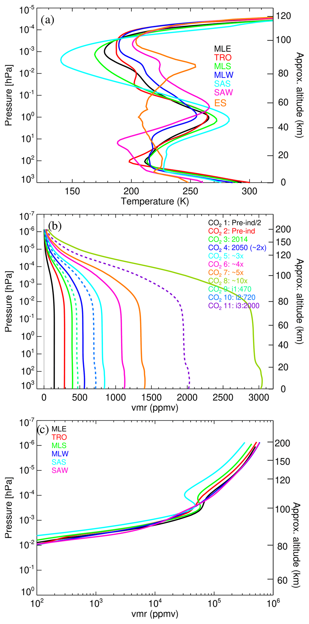
Figure 1 Input data used in the reference calculations. (a) The six temperature profiles used in the reference calculations up to the lower thermosphere (Fig. 7 shows them for the full range of pressures). MLE: mid-latitude equinox (September, 40° N); TRO: tropics (June, Equator); MLS: mid-latitude summer (June, 40° N); MLW: mid-latitude winter (June, 40° S); SAS: subarctic summer (June, 70° N); SAW: subarctic winter (June, 70° S). A profile typical of an elevated stratopause event (ES, mean of MIPAS temperature measured for latitudes of 70–90° N for 15 February 2009) is also shown for comparison and is discussed in Sect. 7.2. (b) CO₂ volume mixing ratio profiles used in this work for the entire altitude range. Solid lines: the profiles used in the reference calculations; dashed lines: intermediate profiles used to test the parameterization. (c) The O(³P) volume mixing ratio profiles. Here and in the following figures, the geometric altitude is approximate, corresponding to the pressure–altitude relationship of the MLE reference atmosphere.

The parameterization computes cooling rates for given inputs of temperature and concentrations of CO₂, O(³P), O₂ and N₂ as a function of pressure. No specific grid is required, and it can be irregular. The routine interpolates the given parameters to its internal pressure grid. Possible cooling effects caused by temperature disturbances at vertical scales smaller than the internal grid of the parameterization, ≲1.75 km (see e.g. Kutepov et al., 2013), are not taken into account. That is, we assume that the cooling induced by non-resolved gravity waves propagating with a vertical wavelength of the order of or smaller than ≲1.75 km would be taken into account in the GCMs by using an appropriate GW (gravity wave) parameterization.

Further, the collisional (de)activation of CO₂(v₂) levels by the main atmospheric molecules (N₂ and O₂) and by O(³P) can also be prescribed. To compute the different coefficients employed by the parameterization (see Sect. 5), reference LTE and non-LTE cooling rates are required (see Sect. 4.1 and 4.2). These are calculated for selected reference atmospheres and are described in the next section.

3 The reference atmospheres

3.1 Temperature

We used the same six pressure–temperature reference atmospheres as in Fomichev et al. (1998) for altitudes below ∼120 km. Above this altitude, they were extended up to ∼200 km with the empirical US Naval Research Laboratory Mass Spectrometer Incoherent Scatter Radar version 2.0 (MSIS2) model (Emmert et al., 2021) for medium conditions of solar activity: F_10.7=103 sfu (June 2011) for all atmospheres except for MLE, which was F_10.7=142 sfu (September 2011). These six p–T profiles cover the envelope of the climatological zonal mean temperatures of the current middle atmosphere very well, e.g. as measured by MIPAS from 2007 to 2012 (see Sect. 7). However, they do not cover the small-scale temporal and spatial temperature variability (see Fig. B6). The performance of the parameterization for such variability is addressed in Sect. 7. Further, the range of the six temperature profiles does not cover the episodes of stratospheric warming with an elevated stratopause well. During these events, the altitude region of the typical stratopause, at about 50 km, is much colder, being even 50 K colder than during normal conditions, and the altitude of the typical mesopause, near 85–90 km, is warmer by a similar amount (see Fig. 1a, profile ES). For these conditions the temperature profile is nearly isothermal from the tropopause up to about 0.1 hPa and exhibits an inversion above, with a peak near the mesopause. We anticipate that, for these rare conditions, the error incurred by this parameterization can be significant (see Sect. 7.2).

We should also mention that the envelope of these reference atmospheres does not fully cover the predicted temperatures for the end of this century for projections with high CO₂ emissions. In particular, WACCM simulations for this century under the RCP6.0 scenario (Marsh, 2011; Marsh et al., 2013; Garcia et al., 2017) yield zonal mean temperatures which are colder in the middle atmosphere. In order to cover such predictions, the envelope of the six p–T profiles assumed here would have to be widened by about −30 K in the upper stratosphere and by about −20 K in the mesosphere. The parameterization accuracy for such predicted temperatures has not been fully assessed in this work as we have considered only the projection of high CO₂ VMR profiles but not the corresponding predicted temperature fields. This will be the subject of future work.

3.2 CO₂, O(³P), O₂ and N₂ abundances

The valid range of the parameterization of Fomichev et al. (1998) with respect to CO₂ volume mixing ratios is exceeded by the CO₂ concentration of several scenarios considered in the 6th Coupled Climate Model Intercomparison Project (CMIP6), in particular for the 4×CO₂ experiment. Several CO₂ scenarios have been proposed for the future. Thus, van Vuuren et al. (2011) proposed the scenario RCP2.6, which reaches tropospheric CO₂ values near 1000 ppmv by the end of the century. Likewise, Meinshausen et al. (2011) suggested the high CO₂ scenario of RCP8.5 (CMIP5), which has CO₂ concentrations of 2000 ppmv in the second half of the 23rd century or even higher than 2000 ppmv (e.g. SSP5-8.5 in CMIP6; see O'Neill et al., 2016). Here we used a wide range of tropospheric CO₂ values ranging from about half of the pre-industrial (1851) value of 285 ppmv to about 10 times this value (see Fig. 1b). The specific profiles were built from a WACCM run under the CMIP6 SSP5-8.5 scenario (Marsh, 2011; Marsh et al., 2013; Garcia et al., 2017). Global annual mean profiles of CO₂ were taken from WACCM simulations for years: 1851 (pre-industrial), CO₂ profile no. 2; 2014, CO₂ profile no. 3; 2050, CO₂ profile no. 4 ($\sim \mathrm{2}\times$pre-industrial); and 2099, CO₂ profile no. 6 ($\sim \mathrm{4}\times$pre-industrial). In addition, we set up the low CO₂ profile (no. 1) by halving pre-industrial profile no. 2, the intermediate CO₂ profile no. 5 ($\sim \mathrm{3}\times$pre-industrial) from the mean of WACCM outputs for 2050 and 2099, the high CO₂ profile no. 7 ($\sim \mathrm{5}\times$pre-industrial) by multiplying WACCM output for 2099 by a factor of 1.25, and the highest CO₂ profile no. 8 ($\sim \mathrm{10}\times$ pre-industrial) by multiplying WACCM output for 2099 by a factor of 2.7. In addition to those CO₂ VMR profiles, we also composed the intermediate profile nos. 9, 10 and 11 for testing the parameterization (see Sect. 6.2), which are shown in Fig. 1b with dashed lines. Profile nos. 9 and 11 were obtained by multiplying WACCM outputs for the years 2050 and 2099 by factors of 0.979 and 1.8, respectively. Profile no. 10 was calculated by weighting the WACCM annual mean for the years 2050 and 2099 by 0.76875 and 0.256250, respectively. WACCM provides the CO₂ VMR profiles up to about 130 km. Above that altitude, they were calculated by using a WACCM-X run for 2008, which provides a CO₂ VMR up to near 500 km, and scaling them, in pressure levels, by the CO₂ value of the corresponding CO₂ profile at a pressure of $\mathrm{5}\times {\mathrm{10}}^{-\mathrm{6}}$ hPa.

As discussed above, the parameterization requires the N₂, O₂ and O(³P) volume mixing ratio profiles for the six p–T reference atmospheres. They were taken from the MSIS2 model (Emmert et al., 2021) and are shown in Fig. S2.

4 Cooling rates for the reference atmospheres

We describe in this section the non-LTE cooling rates used as a reference. To compute the coefficients of the parameterization and the boundaries of the different layers, they also require the calculations of the cooling rates in LTE, which are also described in this section. Further, we have assessed the accuracy of the LTE cooling rates by comparing them with those calculated by an independent code, the Reference Forward Model (RFM, Dudhia, 2017).

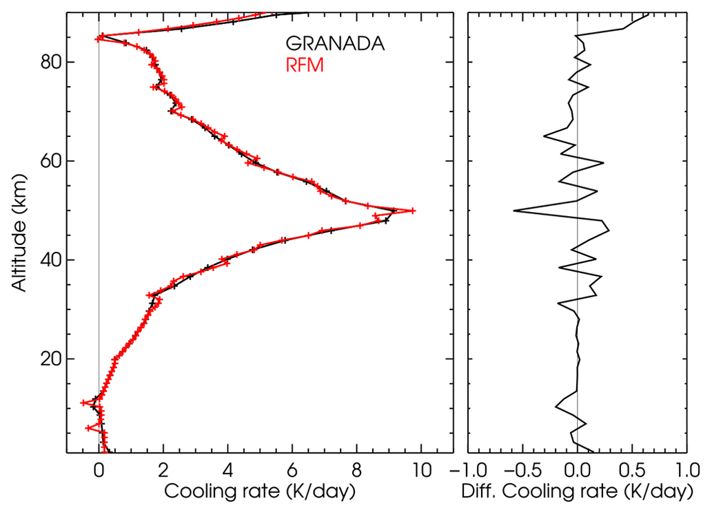
Figure 2 LTE cooling rates for the US standard temperature profile and the CO₂ VMR of Fomichev et al. (1998) computed by the GRANADA algorithm and the RFM code.

4.1 Reference LTE cooling rates

The LTE cooling rates have been computed using a modified Curtis matrix formulation (Funke et al., 2012). In that computation we used as the basis for the radiative transfer calculations (e.g. the optical depths, the transmittances and their differences) the Karlsruhe Optimised and Precise Radiative Transfer Algorithm (KOPRA, Stiller et al., 2002). This code is a well-tested general-purpose line-by-line radiative transfer model that includes all the known relevant processes for performing accurate radiative transfer calculations in planetary atmospheres. We used the CO₂ line list of HITRAN 2016 (Gordon et al., 2017) and the line shapes were modelled with a Voigt profile including the pressure and temperature dependencies of the Doppler and Lorentz half-widths. The line mixing, although of little importance in this case because the transmittances are integrated over a wide spectral range, was also taken into account (see Stiller et al., 2002). The flux transmittances were computed using a 10-point Gaussian quadrature. The wavenumber grid was 0.0005 cm⁻¹. The LTE cooling rates have been computed for the CO₂ bands associated with the vibrational states of the ν₁ν₂ mode manifold covering the spectral range from 540 to 800 cm⁻¹ in intervals of 10 cm⁻¹. All bands listed in HITRAN 2016 for the six most abundant isotopes in those spectral regions were included in the calculation. For reference, the accurate cooling rates computed assuming LTE conditions for the six p–T profiles and the reference eight CO₂ VMRs are shown in Figs. S3 and S4.

In order to ensure the accuracy of these LTE cooling rates, we have compared them with those obtained with another very well-tested and widely used radiative transfer code, RFM (Dudhia, 2017). This code has been used in many studies relevant to the MIPAS instrument (Fischer et al., 2008) and for the retrieval of MIPAS level-2 data obtained by the University of Oxford. It worth mentioning that RFM uses a classical Curtis matrix method (double-flux transmittance differences), while we use the modified Curtis matrix method. Figure 2 shows the results of the comparison for the US standard temperature profile and the CO₂ VMR of Fomichev et al. (1998). Here we used a common fine-altitude grid of 0.5 km. We see that the agreement between both codes is very good, with differences at most of the altitudes smaller than 0.1–0.2 K d⁻¹. Note that some of the major differences appear to be associated with small oscillations in the RFM results.

The same formulation has been used to calculate the Curtis matrices of all the CO₂ ν₂ bands which are required to compute the coefficients of the parameterization in the LTE region (see Sect. 5).

4.2 Reference non-LTE cooling rates

The reference line-by-line non-LTE cooling rates have been computed by using the GRANADA non-LTE code. The details of the method for solving the system of equations for CO₂ are given in Funke et al. (2012). In addition to the solution of the statistical and radiative transfer equations described in that work for the calculation of the non-LTE populations of the CO₂ levels, here, in order to compute accurate non-LTE cooling rates and to account for the overlap between the different CO₂ ν₂ bands, we included an additional final iteration computing the radiation fields in all the bands by using the lambda iteration method. This algorithm shares the radiative transfer algorithm with KOPRA (Stiller et al., 2002). Thus, the details of the radiative transfer calculation related to KOPRA, e.g. line shape, spectroscopic data, wavenumber grid, or line mixing, given in LTE Sect. 4.1 above, also apply to the non-LTE calculations described here.

For this case of non-LTE cooling rates, each ro-vibrational band contributes according to the non-LTE populations of their upper and lower levels. The non-LTE cooling rates calculated here comprise 16 ν₂ vibrational bands emitting and absorbing in the 15 µm region, i.e. the fundamental ν₂ band, three first hot ν₂ bands, seven second ν₂ hot bands of the major CO₂ isotopologue and ν₂ fundamental bands of isotopologues ¹⁶O¹³C¹⁶O, ¹⁶O¹²C¹⁸O, ¹⁶O¹²C¹⁷O, ¹⁶O¹³C¹⁸O and ¹⁶O¹³C¹⁷O. The contributions of other weaker ν₂ bands arising from higher v₂ levels, e.g. v₂=4, 5 or 6, are included in the calculation but have negligible contributions for the conditions of Earth's atmosphere.

Funke et al. (2012)

Table 1 The main collisional processes affecting the CO₂ vibrational levels included in the calculations of the non-LTE cooling rates (extracted from Table 5 of Funke et al., 2012).

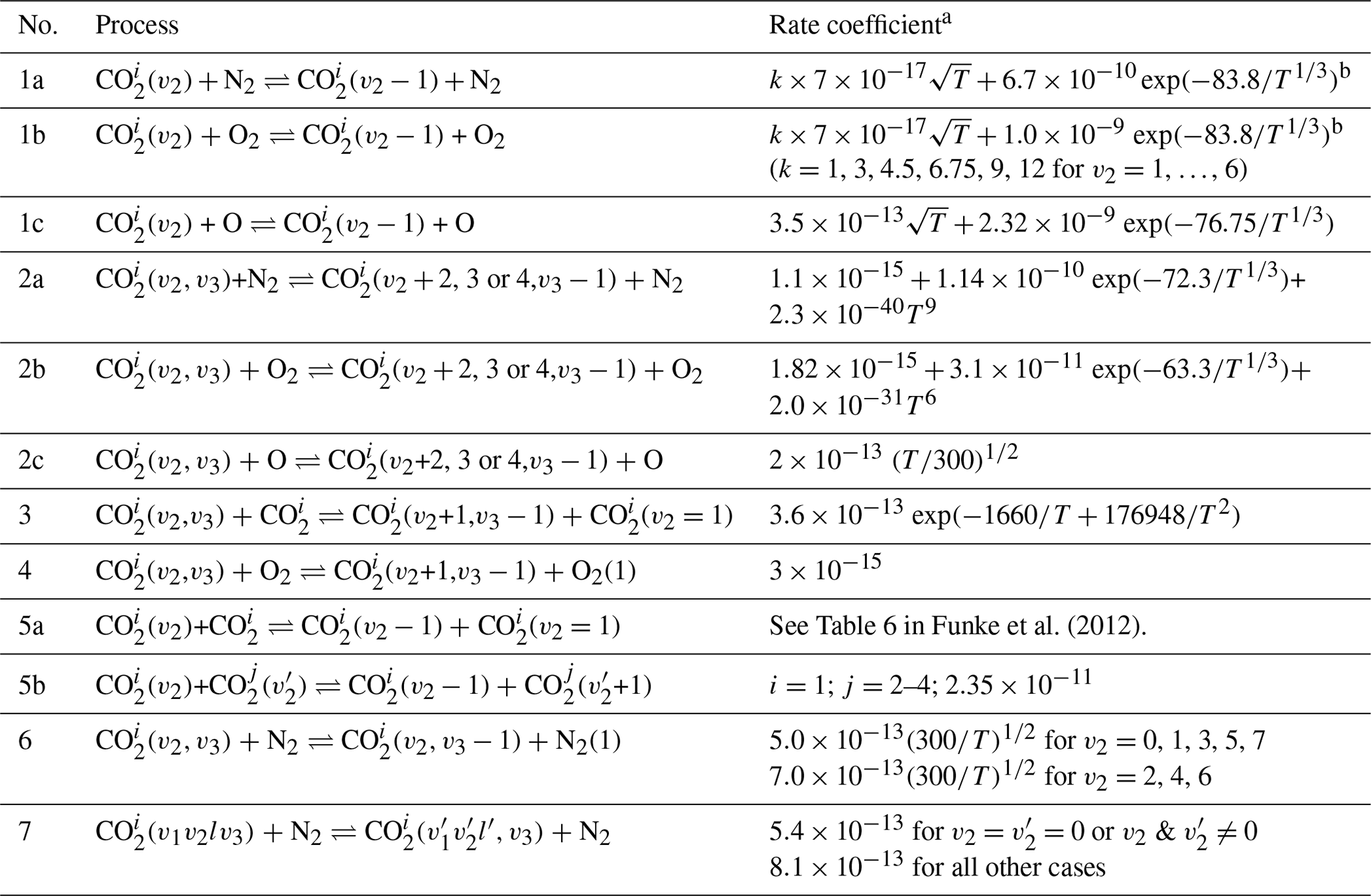
^a Rate coefficient for the forward sense of the process (cm³ s⁻¹). ^b This rate is taken as 10⁻¹⁵ cm³ s⁻¹ for temperatures lower than 150 K (see Funke et al., 2012). T is temperature (K). i and j are different CO₂ isotopologues. i=1–6 except as noted. v₂ denotes equivalent 2v₁+v₂ states: for example, v₂=2 is the triad (10002, 02201, 10001).

For the calculations of the non-LTE cooling rates, a collisional scheme and collisional rates are required. Although the collisional rates affecting the CO₂ v₂ levels are an input parameter for the parameterization, here we have used, for the calculations of the reference cooling rates and for testing the parameterization, the collisional rates described in Funke et al. (2012). They have been recently revised and used in the non-LTE retrieval of temperature from SABER and MIPAS measurements (García-Comas et al., 2008, 2023). The most relevant collisional processes concerning the populations of the levels emitting in the different ν₂ bands described above, and their rates, are listed in Table 1 for easier reference. We should note that these rates and their temperature dependencies are different from those used in the previous parameterization of Fomichev et al. (1998). The values are in general of very similar magnitudes, except for the k_O rate (process 1c in Table 1) that has been considered here with its upper limit, i.e. about a factor of 2 larger than in the parameterization of Fomichev et al. (1998). This rate coefficient is not well known, with uncertainties of the order of a factor of 2 (see e.g. García-Comas et al., 2008). While laboratory measurements are in the range of 1.5 to $\mathrm{2}\times {\mathrm{10}}^{-\mathrm{12}}$ cm³ s⁻¹, the values derived from atmospheric observations are close to $\mathrm{6}\times {\mathrm{10}}^{-\mathrm{12}}$ cm³ s⁻¹. Although this rate can be chosen when using this parameterization, we have optimized it for its larger value (see Table 1), as this rate has been used in the most recent non-LTE retrievals of temperature from SABER and MIPAS measurements. The effects of using half of this value on the cooling rates are discussed in Sect. 6.2. In the comparisons shown in the next sections, we consistently used the collisional rates in Table 1 for the two parameterizations.

The cooling rates near 15 µm change very little with the illumination conditions. However, those cooling rates (or more strictly speaking, the flux divergence) of the CO₂ ν₂ bands computed by GRANADA under daytime conditions are affected by some emission from the relaxation and/or redistribution of the solar energy absorbed in the near-infrared bands (see e.g. López-Puertas et al., 1990). As this absorption or heating is already taken into account by the near-infrared (NIR) solar heating parameterization (see Sect. 9), all the non-LTE cooling rates computed here have been performed for nighttime conditions.

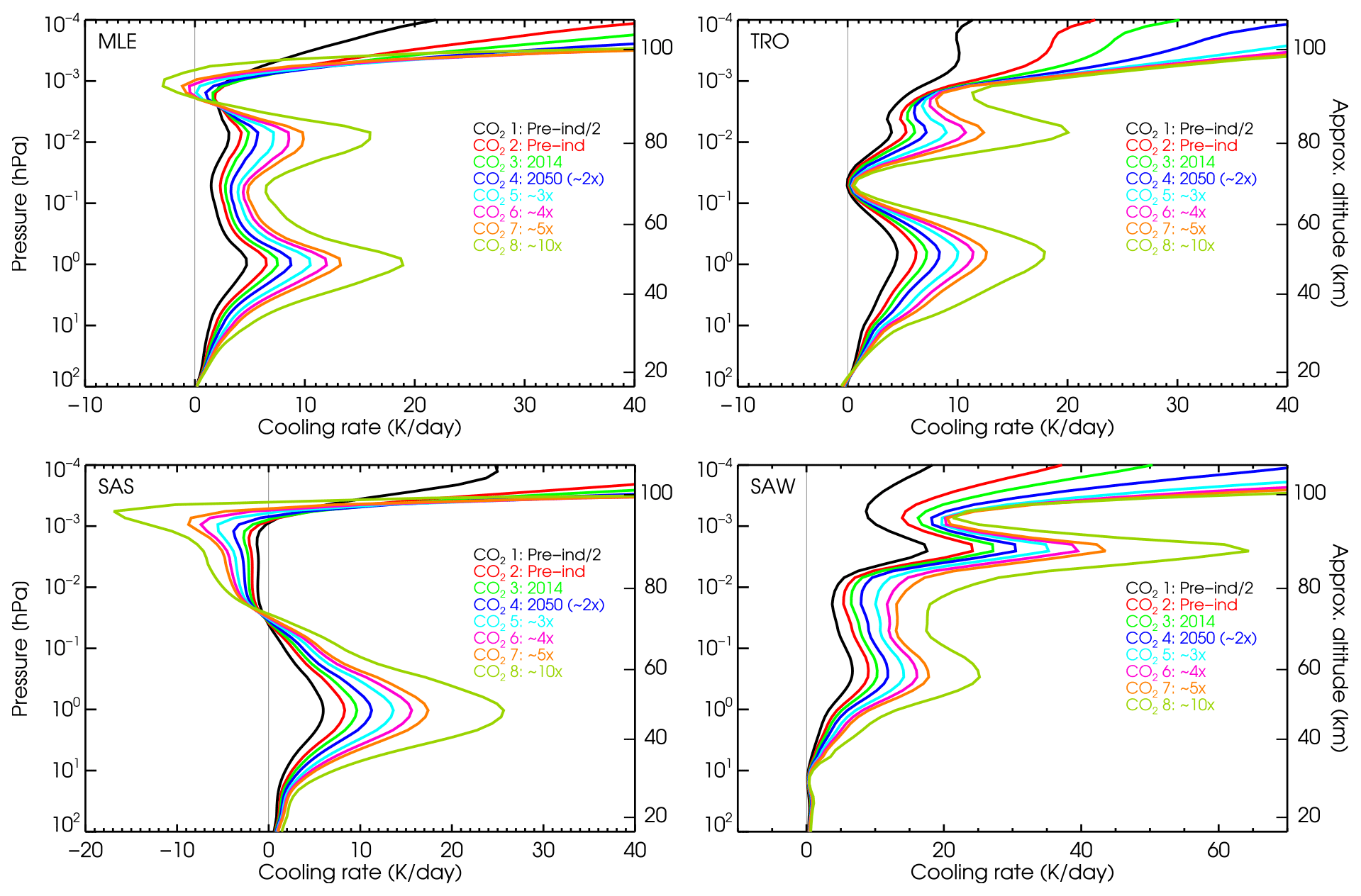
Figure 3 The non-LTE cooling rates for four reference atmospheres shown for altitudes up to the lower thermosphere. The cooling rates extended to the thermosphere are shown in Fig. S5. Note the different x scales.

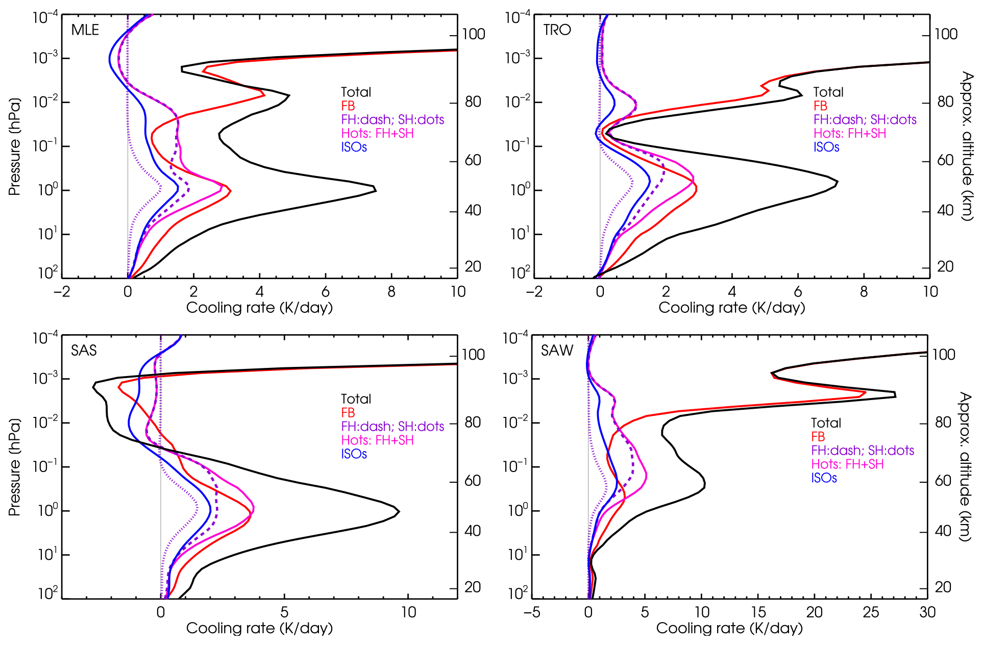
Figure 4 Contributions of the different CO₂ bands to the cooling rates for four p–T reference atmospheres and the contemporary CO₂ VMR no. 3 profile. Note the different x scales.

The results for the accurate, line-by-line non-LTE cooling rates computed for the six reference p–T profiles and the eight CO₂ VMRs are shown in Fig. 3 from the stratosphere up to the lower thermosphere and in Fig. S5 for the upper part of the parameterization, i.e. from 80 to 200 km. We observe that the altitude distribution of the cooling rates depends very much on the temperature profile. This is the major difficulty in building the parameterization. A general common feature is the maximum near the stratopause, because at these altitudes the non-LTE cooling rates do not differ significantly from those in LTE, and these are mainly driven by the high temperature of this region. Above the stratopause, the total non-LTE cooling rates depend very much on the contributions of the different bands, e.g. the ν₂ fundamental band of the major isotopologue (FB), the contributions of the first and hot bands (Hots) and those of the ν₂ fundamental bands of the five minor isotopologues. These contributions are shown in Fig. 4 for the contemporary CO₂ VMR profile (no. 3) and four p–T profiles. The non-LTE cooling rates generally decrease with altitude above the stratopause, reaching a minimum near the mesopause for several p–T profiles; see e.g. the SAS and MLE atmospheres in Figs. 3 and 4. The cooling can even be negative, e.g. heating for the very cold sub-arctic summer (SAS) mesopause, where heating can be several Kelvin per day (see the bottom-left panel of Fig. 3). Exceptional cases are the winter atmospheres (mid-latitude winter, MLW (not shown), and sub-arctic winter, SAW), where the mesopause is warmer and the cooling rates are high in this region. Above the mesopause, the cooling rate rapidly increases following the enhancement of the kinetic temperature. Above about 130 km, however, the cooling rates decline (see Fig. B1). At these altitudes, cooling to space is a very good approximation to the non-LTE cooling rate, which, when expressed in Kelvin per day, is proportional to the CO₂ VMR, to the atomic oxygen density [O] and to the temperature through $\exp (-E/kT)$ (see e.g. Sect. 9.2 in López-Puertas and Taylor, 2001). As altitude increases, the CO₂ VMR decreases, and so does [O]. These two effects overcome the temperature increase, leading to a net cooling rate decrease. Note the significant contribution of the hot bands in the lower thermosphere (120–150 km; see Fig. B1), essentially due to the first hot band of the major isotopologue at these altitudes, which is about 10 % of the total cooling.

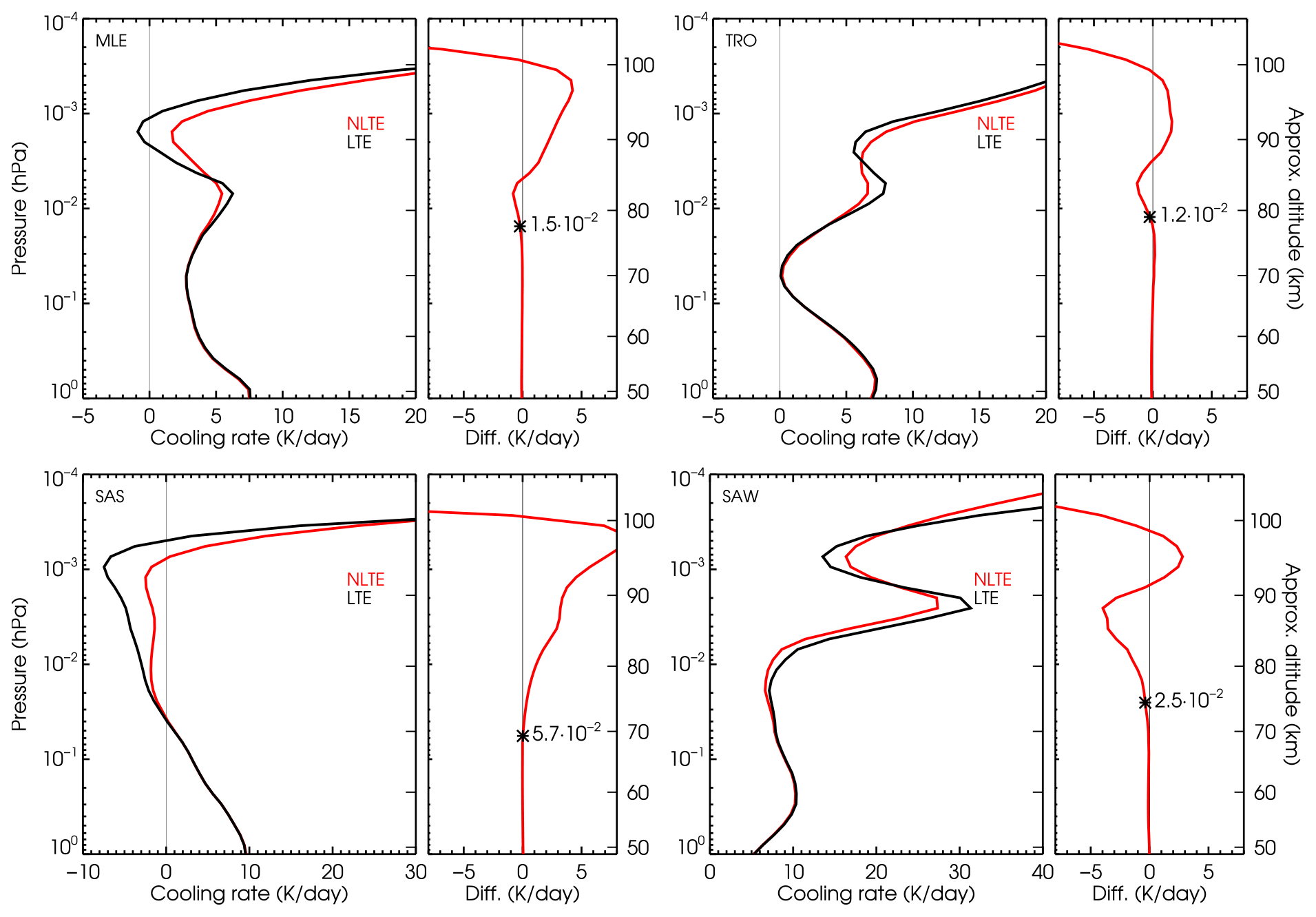
Figure 5 Non-LTE–LTE cooling rate differences for four p–T reference atmospheres and the contemporary CO₂ VMR no. 3 profile. Differences for the higher CO₂ VMR no. 6 profile ($\sim \mathrm{4}\times$ the pre-industrial profile) are shown in Fig. S6. The “*” symbol indicates the pressure level (hPa) where the non-LTE–LTE difference reaches 5 %. Note the different x scales.

The dependence of the non-LTE cooling rates on the CO₂ abundances is illustrated in Fig. 3. We observe that, in general, the cooling rate correlates very well with the CO₂ abundance, although that correlation is not always linear and generally depends on altitude. This is also true for the cases where we have net heating for low CO₂ VMR, e.g. the SAS atmosphere between about 75 km and 95 km. For the MLE and MLS atmospheres, the cooling rate near ∼90 km changes from net cooling to net heating for the largest CO₂ VMRs. Further, the very low cooling for the tropical (TRO) p–T profile near 70 km remains very low even when the CO₂ VMR varies by a factor of 20. In the lower thermosphere, e.g. above around ∼110 km, however, the dependency of the cooling rate on the CO₂ is very close to being linear (see Fig. S5).

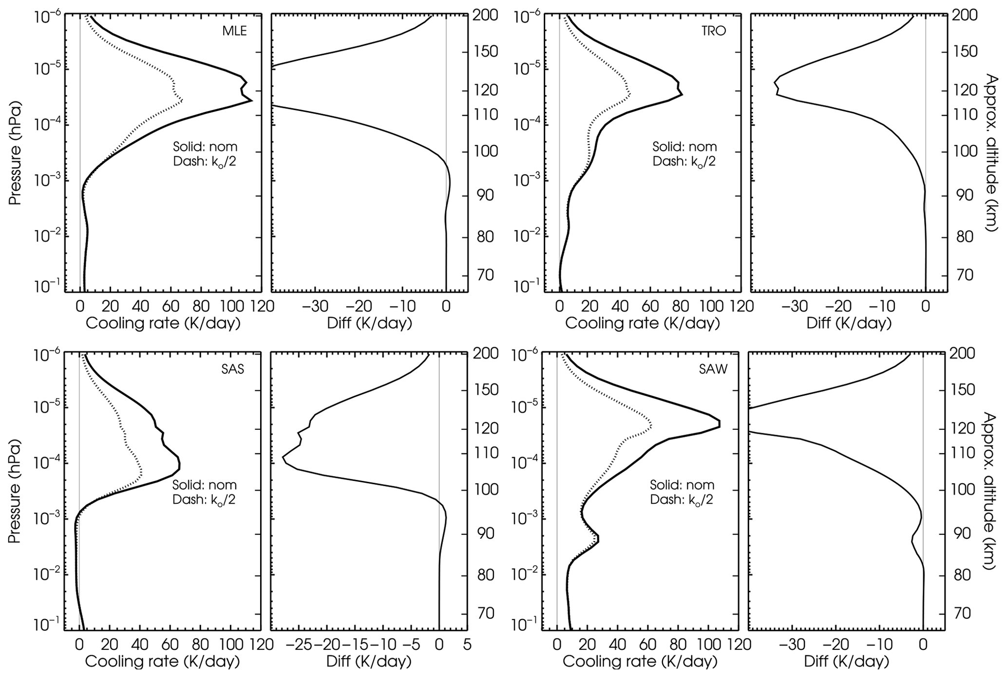
Figure 6 Effect of the k_O collisional rate (or, equivalently, the O(³P) concentration) on the non-LTE cooling rates for four p–T reference atmospheres and the contemporary CO₂ VMR no. 3 profile. Note the different x scales.

A comparison of the non-LTE and LTE cooling rates for the six p–T reference atmospheres for CO₂ VMR nos. 3 (current VMR) and 6 (4 times the pre-industrial value) is shown in Figs. 5 and S6. This comparison is necessary in order to establish the boundaries of the different atmospheric regions of the parameterization (see Sect. 5). We first observe (Fig. 5) that the altitude of the departure of the cooling rate from LTE (considered the altitude where the non-LTE–LTE difference is larger than 5 %) depends on the temperature profile and ranges from $\mathrm{5.2}\times {\mathrm{10}}^{-\mathrm{2}}$ hPa (∼72.5 km) for the SAS atmosphere to $\mathrm{1.2}\times {\mathrm{10}}^{-\mathrm{2}}$ hPa (∼78.7 km) for the TRO atmosphere. A similar plot but for the higher CO₂ profile no. 6 ($\sim \mathrm{4}\times$ pre-industrial) is shown in Fig. S6. An overview of the altitude or pressure level of the deviation of the cooling rate from LTE is shown in Fig. B2 for the six p–T profiles and the eight CO₂ VMR profiles. We see that the lower altitudes (higher pressures) occur for the SAS and SAW reference atmospheres. It is also evident that this altitude increases with the CO₂ VMR, except for the SAS and SAW cases, for which it is nearly independent of the CO₂ VMR. That is expected as, for a more abundant CO₂ atmosphere, the 15 µm bands become optically thicker and fewer collisions are sufficient for keeping the emitting levels in LTE. Figure B2 suggests that, for higher CO₂ VMRs, the LTE–non-LTE transition region could be placed at higher altitudes. However, as the parameterization is intended to cover the full range of CO₂ VMR profiles, we have to be conservative, and we placed it at the lowest altitude for any p–T or CO₂ VMR profile. Thus, it has been taken at x=9.875 ($p=\mathrm{5.14}\times {\mathrm{10}}^{-\mathrm{2}}$ hPa, z≈70 km), which, except for the SAW atmosphere with the lowest CO₂ profile, fulfils the LTE–non-LTE transition region for all the p–T and CO₂ VMR profiles.

For completeness, Fig. B3 shows an example of the comparison of non-LTE and LTE cooling rates, including the thermosphere for the six p–T profiles and the current CO₂ values. This shows the enormous difference between LTE and non-LTE cooling rates (non-LTE values being much smaller) in the thermosphere.

The atomic oxygen concentration is an input to the parameterization and plays a crucial role in determining the CO₂ infrared cooling. As a consequence, it is very important in establishing the different non-LTE regions of the parameterization (Fomichev et al., 1998). To identify the atmospheric regions where it is important, we have performed a calculation by dividing the k_O collisional rate by a factor of 2, which is almost equivalent to changing the O(³P) concentration by the same factor. Figure 6 shows this effect for four p–T profiles and considering the current CO₂. Generally, it is most important above around 10⁻³ hPa (∼95 km). However, for the SAS and SAW atmospheres, it is also important down to $\mathrm{5}\times {\mathrm{10}}^{-\mathrm{3}}$ hPa (∼85 km). The fact that its importance starts being significant at different atmospheric levels for the different p–T profiles poses an additional difficulty in the development of the parameterization.

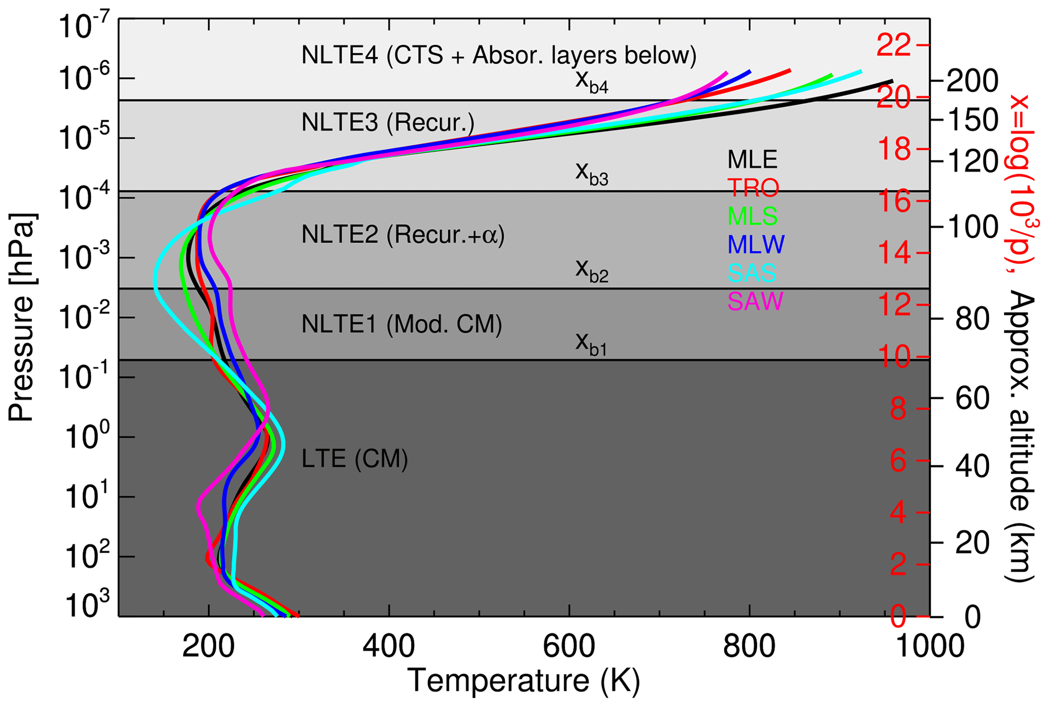
Figure 7 Atmospheric regions considered in the parameterization. x_b,i represents the boundaries of the layers: $x_{b,\mathrm{1}}=\mathrm{9.875}$, $x_{b,\mathrm{2}}=\mathrm{12.625}$, $x_{b,\mathrm{3}}=\mathrm{16.375}$ and $x_{b,\mathrm{4}}=\mathrm{19.875}$. The temperature profiles used in the reference calculations are also shown as a reference.

5 The parameterization

Essentially, here we follow the parameterization developed by Fomichev et al. (1998). A brief description of the method, including the most important features and equations, is given in this section.

The atmosphere is divided into five different regions (see Fig. 7) where different approaches are used for calculating the cooling rates. These regions are qualitatively the same as those defined by Fomichev et al. (1998), but their altitude extensions (except for the LTE region) have been significantly revised, mainly as a consequence of the ample range of CO₂ abundances for which this parameterization is developed. In fact, their upper boundaries have been moved upwards (except for LTE), resulting in the following ranges: LTE x=0–9.875 (z=0–≈70 km), NLTE1 x=9.875–12.625 (z≈70–87 km), NLTE2 x=12.625–16.375 (z≈87–109 km), NLTE3 x=16.375–19.875 (z≈109–180 km) and NLTE4 x>19.875 (z≳180 km).

The lowermost (LTE) and uppermost (NLTE4) regions are the most straightforward and also the regions where the errors are in general smaller. The most difficult parts are the transition regions from LTE to non-LTE, where (i) several bands contribute to the cooling with different source functions and their relative contributions depend very much on the actual temperature profiles (see Fig. 4), and (ii) the exchange of radiation between the layers is significant and different for the considered bands. Further, although most of the radiative excitation at a given layer is produced by the absorption of photons travelling from below, the absorption of photons travelling downwards can also contribute significantly. This is the case, for example, for the stronger fundamental band near the mesopause. Further, the cooling above around 90 km also depends on the collisions with atomic oxygen. This effect can be accurately taken into account in the upper non-LTE regions where all the bands become optically thin. However, it is very difficult to represent it properly between around the mesopause and a few tens of kilometres above, where the atomic oxygen concentration varies largely and the exchange of radiation between the layers is still important.

5.1 The LTE region

The parameterization in the LTE region is based on the Curtis matrix method. The cooling rate ${\mathit{ϵ}}_i^t\left(\mathit{\nu }\right)$ at a given pressure level x_i, in a spectral region ν and for a particular temperature profile t is given by

$$\begin{array}{}\text{(1)}& {\mathit{ϵ}}_i^t\left(\mathit{\nu }\right)=\sum _{j=\mathrm{0}}^{j_{\mathrm{CM}}}{\mathcal{A}}_{i,j}^t\left(\mathit{\nu }\right){\mathit{\phi }}_j^t\left(\mathit{\nu }\right)+v_i^t\left(\mathit{\nu }\right)\mathit{\phi }(T_{\mathrm{surf}}^t,\mathit{\nu }),\end{array}$$

where the indices i,j refer to pressure levels x_i and x_j, and the sum is extended over pressure levels x_j ranging from the lower boundary, x_j=0, until $x_{j_{\mathrm{CM}}}=\mathrm{13.875}$. This upper boundary of the Curtis matrix has been selected to minimize the error in the lowest non-LTE region, NLTE1 (see more details in Sect. 5.2 below). ${\mathcal{A}}_{i,j}^t\left(\mathit{\nu }\right)$ is the modified Curtis matrix (slightly different from its usual definition; see e.g. López-Puertas and Taylor, 2001). The factor ${\mathit{\phi }}_j^t\left(\mathit{\nu }\right)$ in Eq. (1) represents the exponential part of the Planck function and is given by

$$\begin{array}{}\text{(2)}& {\mathit{\phi }}_j^t\left(\mathit{\nu }\right)=\exp [-h\mathit{\nu }/(k_{\mathrm{B}}{T}_j^t\left)\right],\end{array}$$

where h is the Planck constant, k_B is the Boltzmann constant, and $T_j^t$ is the temperature of the p–T profile t at level x_j. Similarly, $\mathit{\phi }(T_{\mathrm{surf}}^t,\mathit{\nu })$ corresponds to the exponential part of the Planck function for the surface temperature $T_{\mathrm{surf}}^t$. The $v_i^t\left(\mathit{\nu }\right)$ term accounts for the absorption at level i times the transmission from the surface up to level i at ν, so that $v_i^t\left(\mathit{\nu }\right)\mathit{\phi }(T_{\mathrm{surf}}^t,\mathit{\nu })$ accounts for the heating rate due to the absorption of the radiation from the surface (or lower boundary). The cooling rate is calculated in the spectral range from 540 to 800 cm⁻¹ divided into frequency intervals, ν, 10 cm⁻¹ wide. Those LTE cooling rate profiles have been calculated for each of the six p–T reference atmospheres and the eight CO₂ VMR profiles.

In the parameterization, the Curtis matrix is expressed with an explicit temperature dependence by

$${\mathcal{A}}_{i,j}^t\left(\mathit{\nu }\right)={\mathbf{a}}_{i,j}^t\left(\mathit{\nu }\right)+{\mathbf{b}}_{i,j}^t\left(\mathit{\nu }\right){\mathit{\phi }}_i^t\left(\mathit{\nu }\right),$$

where the matrix coefficients ${\mathbf{a}}_{i,j}^t\left(\mathit{\nu }\right)$ and ${\mathbf{b}}_{i,j}^t\left(\mathit{\nu }\right)$ are given by

$$\begin{array}{c}{\displaystyle }{\mathbf{a}}_{i,j}^t\left(\mathit{\nu }\right)={\mathcal{A}}_{i,j}^t\left(\mathit{\nu }\right){\displaystyle \frac{S_{\mathrm{0}}\left(\mathit{\nu }\right)}{S_{\mathrm{0}}\left(\mathit{\nu }\right)+\left[S_{\mathrm{1}}\right(\mathit{\nu })+S_{\mathrm{2}}(\mathit{\nu }\left)\right]{\mathit{\phi }}_i^t\left(\mathit{\nu }\right)}},\\ {\displaystyle }{\mathbf{b}}_{i,j}^t\left(\mathit{\nu }\right)={\mathcal{A}}_{i,j}^t\left(\mathit{\nu }\right){\displaystyle \frac{S_{\mathrm{1}}\left(\mathit{\nu }\right)+S_{\mathrm{2}}\left(\mathit{\nu }\right)}{S_{\mathrm{0}}\left(\mathit{\nu }\right)+\left[S_{\mathrm{1}}\right(\mathit{\nu })+S_{\mathrm{2}}(\mathit{\nu }\left)\right]{\mathit{\phi }}_i^t\left(\mathit{\nu }\right)}},\end{array}$$

and S₀(ν), S₁(ν) and S₂(ν) are the band strengths of the fundamental, first hot and second hot bands, respectively, in the ν interval. In this way, the temperature dependence, mainly caused by the band strength of the first and second hot bands, is carried out in ${\mathit{\phi }}_i^t\left(\mathit{\nu }\right)$. Those matrix coefficients are calculated for each spectral interval ν. We obtain the coefficients for the entire spectral region of the CO₂ 15 µm bands by summing over all the ν intervals and weighting with the ν dependency of the ${\mathit{\phi }}_i^t\left(\mathit{\nu }\right)/{\mathit{\phi }}_i^t\left({\mathit{\nu }}_{\mathrm{0}}\right)$ factor, e.g.

$${\mathbf{a}}_{i,j}^t={\displaystyle \frac{{\sum }_{\mathit{\nu }}{\mathbf{a}}_{i,j}^t\left(\mathit{\nu }\right){\mathit{\phi }}_j^t\left(\mathit{\nu }\right)}{{\mathit{\phi }}_j^t\left({\mathit{\nu }}_{\mathrm{0}}\right)}}\text{ and }{\mathbf{b}}_{i,j}^t={\displaystyle \frac{{\sum }_{\mathit{\nu }}{\mathbf{b}}_{i,j}^t\left(\mathit{\nu }\right){\mathit{\phi }}_j^t\left(\mathit{\nu }\right){\mathit{\phi }}_i^t\left(\mathit{\nu }\right)}{{\mathit{\phi }}_j^t\left({\mathit{\nu }}_{\mathrm{0}}\right){\mathit{\phi }}_i^t\left({\mathit{\nu }}_{\mathrm{0}}\right)}},$$

with ν₀=667.3799 cm⁻¹ being the frequency of the fundamental band of the major isotopologue.

Next, we define global a_i,j and b_i,j matrix coefficients, to be used for any input temperature profile, as weighted averages of ${\mathbf{a}}_{i,j}^t$ and ${\mathbf{b}}_{i,j}^t$ for the six reference p–T profiles. We introduce a set of normalized weights ${\mathit{\xi }}_i^t$, altitude-dependent, for each temperature profile so that

$$\begin{array}{}\text{(3)}& {\mathbf{a}}_{i,j}=\sum _t{\mathit{\xi }}_i^t{\mathbf{a}}_{i,j}^t\text{ and }{\mathbf{b}}_{i,j}=\sum _t{\mathit{\xi }}_i^t{\mathbf{b}}_{i,j}^t.\end{array}$$

Analogously to the matrix coefficients ${\mathbf{a}}_{i,j}^t\left(\mathit{\nu }\right)$ and ${\mathbf{b}}_{i,j}^t\left(\mathit{\nu }\right)$, we define the corresponding vector coefficients for the surface flux, $a_{\mathrm{surf},i}^t\left(\mathit{\nu }\right)$ and $b_{\mathrm{surf},i}^t\left(\mathit{\nu }\right)$, so that

$$v_i^t\left(\mathit{\nu }\right)=a_{\mathrm{surf},i}^t\left(\mathit{\nu }\right)+b_{\mathrm{surf},i}^t\left(\mathit{\nu }\right){\mathit{\phi }}_i^t\left(\mathit{\nu }\right),$$

with

$$\begin{array}{c}{\displaystyle }{a}_{\mathrm{surf},i}^t\left(\mathit{\nu }\right)={\displaystyle \frac{v_i^t\left(\mathit{\nu }\right)S_{\mathrm{0}}\left(\mathit{\nu }\right)}{S_{\mathrm{0}}\left(\mathit{\nu }\right)+\left[S_{\mathrm{1}}\right(\mathit{\nu })+S_{\mathrm{2}}(\mathit{\nu }\left)\right]{\mathit{\phi }}_i^t\left(\mathit{\nu }\right)}},\\ {\displaystyle }{b}_{\mathrm{surf},i}^t\left(\mathit{\nu }\right)={\displaystyle \frac{v_i^t\left(\mathit{\nu }\right)\left[S_{\mathrm{1}}\right(\mathit{\nu })+S_{\mathrm{2}}(\mathit{\nu }\left)\right]}{S_{\mathrm{0}}\left(\mathit{\nu }\right)+\left[S_{\mathrm{1}}\right(\mathit{\nu })+S_{\mathrm{2}}(\mathit{\nu }\left)\right]{\mathit{\phi }}_i^t\left(\mathit{\nu }\right)}},\\ {\displaystyle }{a}_{\mathrm{surf},i}^t={\displaystyle \frac{{\sum }_{\mathit{\nu }}{a}_{\mathrm{surf},i}^t\left(\mathit{\nu }\right)\mathit{\phi }(T_{\mathrm{surf}}^t,\mathit{\nu })}{\mathit{\phi }(T_{\mathrm{surf}}^t,{\mathit{\nu }}_{\mathrm{0}})}},\\ {\displaystyle }{b}_{\mathrm{surf},i}^t\left(\mathit{\nu }\right)={\displaystyle \frac{{\sum }_{\mathit{\nu }}{b}_{\mathrm{surf},i}^t\left(\mathit{\nu }\right)\mathit{\phi }(T_{\mathrm{surf}}^t,\mathit{\nu }){\mathit{\phi }}_i^t\left(\mathit{\nu }\right)}{\mathit{\phi }(T_{\mathrm{surf}}^t,{\mathit{\nu }}_{\mathrm{0}}){\mathit{\phi }}_i^t\left({\mathit{\nu }}_{\mathrm{0}}\right)}}.\end{array}$$

$$\begin{array}{}\text{(4)}& a_{\mathrm{surf},i}=\sum _t{\mathit{\xi }}_i^t{a}_{\mathrm{surf},i}^t\text{ and }{b}_{\mathrm{surf},i}=\sum _t{\mathit{\xi }}_i^t{b}_{\mathrm{surf},i}^t.\end{array}$$

In this way, the cooling rate ϵ_i, at a pressure level x_i, for a given input temperature profile T_inp is calculated in the parameterization by

$$\begin{array}{}\text{(5)}& \begin{array}{rl}{\mathit{ϵ}}_i& =\sum _j\mathit{\left\{}\left[{\mathbf{a}}_{i,j}+{\mathbf{b}}_{i,j}{\mathit{\phi }}_i^{T_{\mathrm{inp}}}\left({\mathit{\nu }}_{\mathrm{0}}\right)\right]{\mathit{\phi }}_j^{T_{\mathrm{inp}}}\right({\mathit{\nu }}_{\mathrm{0}}\left)\mathit{\right\}}\\ & +\left[a_{\mathrm{surf},i}+b_{\mathrm{surf},i}{\mathit{\phi }}_i^{T_{\mathrm{inp}}}\left({\mathit{\nu }}_{\mathrm{0}}\right)\right]\mathit{\phi }(T_{\mathrm{surf}}^{inp},{\mathit{\nu }}_{\mathrm{0}}).\end{array}\end{array}$$

The weights ${\mathit{\xi }}_i^t$ are obtained by minimizing the cost function χ(x_i) at each pressure level x_i, given by the sum of the square of the differences of the reference LTE cooling rates, ${\mathit{ϵ}}_{\mathrm{ref}}^t$, and those computed by the parameterization by using Eq. (5), ${\mathit{ϵ}}_{\mathrm{par},i}^t$, for each p–T profile t, e.g.

$$\mathit{\chi }\left(x_i\right)=\sum _t{\mathit{\eta }}^t\mathit{\{}{\mathit{ϵ}}_{\mathrm{ref},i}^t-{\mathit{ϵ}}_{\mathrm{par},i}^t{\mathit{\}}}^{\mathrm{2}},$$

or, in more detail, by

$$\begin{array}{rl}\mathit{\chi }\left(x_i\right)& =\sum _t{\mathit{\eta }}^t\mathit{\{}{\mathit{ϵ}}_{\mathrm{ref},i}^t-\mathit{\{}\sum _j\sum _{t^{\prime }}{\mathit{\xi }}_i^{t^{\prime }}\left[{\mathbf{a}}_{i,j}^{t^{\prime }}+{\mathbf{b}}_{i,j}^{t^{\prime }}{\mathit{\phi }}_i^t\left({\mathit{\nu }}_{\mathrm{0}}\right)\right]\\ & \cdot {\mathit{\phi }}_j^t\left({\mathit{\nu }}_{\mathrm{0}}\right)+\left[a_{\mathrm{surf},i}^{t^{\prime }}+b_{\mathrm{surf},i}^{t^{\prime }}{\mathit{\phi }}_i^t\left({\mathit{\nu }}_{\mathrm{0}}\right)\right]\mathit{\phi }(T_{\mathrm{surf}}^t,{\mathit{\nu }}_{\mathrm{0}})\mathit{\}}{\mathit{\}}}^{\mathrm{2}}.\end{array}$$

The normalized coefficients η^t were originally introduced to consider different fractions of the area of Earth ascribed to each p–T reference profile. Thus, in the previous parameterization they were taken to be equal to 0.05 for the subarctic (winter and summer) profiles, 0.1 for the mid-latitude (winter and summer) profiles, 0.4 for the tropical profile and 0.3 for the mid-latitude equinox p–T profile. In this study, we have explored different options including the original coefficients and a uniform weighting for the six p–T profiles, and we found a smaller χ for the latter, e.g. $\mathit{\eta }=\mathrm{1}/\mathrm{6}$ for all the profiles. Hence, that was included in this version.

In that way, we have parameterized the cooling rates as a function of temperature. The cooling rates also depend on the CO₂ VMR profiles (see Fig. 3). The parameterization incorporates the dependence on the CO₂ abundance by calculating a_i,j and b_i,j for a generic CO₂ profile by assuming a linear interpolation in $\log [{\mathbf{a}}_{i,j}/\mathrm{VMR}(x_i\left)\right]$ and $\log [{\mathbf{b}}_{i,j}/\mathrm{VMR}(x_i\left)\right]$ from the adjacent CO₂ VMR profiles. Thus, the a_i,j and b_i,j coefficients of Eq. (3) have been calculated (and are provided) for the eight CO₂ VMRs shown in Fig. 1b.

5.2 The NLTE1 region: the transition from LTE to non-LTE

This region is difficult to parameterize because we have several bands contributing to the cooling (see Fig. 4), and their relative contributions depend significantly on both the temperature structure and the CO₂ VMR profile. Note that, at certain levels, the cooling induced by the weaker hot bands is larger than that of the stronger fundamental band. We should also note that the contribution of the first hot bands at high altitudes, ∼110–150 km, is not negligible (5 %–10 %, Fig. B1). This contribution is accounted for in the parameterization by implicitly assuming that it is produced by the fundamental band of the main isotopologue (see below and Sect. 4.2).

The lower boundary of this region, i.e. the LTE–NLTE1 transition, occurs, depending on the temperature profile, at altitudes from ∼70 km up to ∼85 km (0.08 to 0.004 hPa; see Fig. B2), taking place a few kilometres lower for the subarctic summer atmosphere and the lowest CO₂ VMR. This transition region occurs at higher altitudes for larger CO₂ VMRs. That is, the atmosphere becomes optically thicker and fewer collisions are enough to keep the levels in LTE. However, since we also need to represent the low CO₂ VMRs, we decided to conservatively set up this region at rather low altitudes, $x_{b,\mathrm{1}}=\mathrm{9.875}$ (∼70 km), the same level used in the previous parameterization.

The upper limit of this region was set up in the previous parameterization at the pressure levels where collisions with O(³P) start affecting the cooling rates significantly. Again, that pressure level depends on the temperature profile (and also on the O(³P) concentration), being lower at ∼0.004 hPa (x≈12.4), for the subarctic summer and winter conditions (see Fig. 6). Here, we have taken the upper boundary of $x_{b,\mathrm{2}}=\mathrm{12.625}$ (≈87 km), slightly higher than the 12.5 value assumed in the original parameterization.

In this region we followed, as in Fomichev et al. (1998), the matrix approach discussed in Sect. 5.1 above. Thus, Eq. (5) was used but with modified ${\mathbf{a}}_{i,j}^{\prime t}$ and ${\mathbf{b}}_{i,j}^{\prime t}$ coefficients that account for the non-LTE corrections. For each p–T profile, t, we define

$${\mathbf{a}}_{i,j}^{\prime t}={\mathbf{a}}_{i,j}^t\left[{\mathit{ϵ}}_{(\mathrm{ref},\mathrm{nlte}),i}^t/{\mathit{ϵ}}_{(\mathrm{ref},\mathrm{lte}),i}^t\right]$$

and

$${\mathbf{b}}_{i,j}^{\prime t}={\mathbf{b}}_{i,j}^t\left[{\mathit{ϵ}}_{(\mathrm{ref},\mathrm{nlte}),i}^t/{\mathit{ϵ}}_{(\mathrm{ref},\mathrm{lte}),i}^t\right],$$

where ${\mathit{ϵ}}_{(\mathrm{ref},\mathrm{lte})}^t$ and ${\mathit{ϵ}}_{(\mathrm{ref},\mathrm{nlte})}^t$ are the reference LTE and non-LTE cooling rates, respectively. Then, the general ${\mathbf{a}}_{i,j}^{\prime }$ and ${\mathbf{b}}_{i,j}^{\prime }$ coefficients were calculated by following the same procedure as for the LTE region, i.e. by weighting the p–T-specific ${\mathbf{a}}_{i,j}^{\prime t}$ and ${\mathbf{b}}_{i,j}^{\prime t}$ coefficients with a set of altitude-dependent weights ${\mathit{\xi }}_i^{\prime t}$ and minimizing the total cost function χ(x_i) (see Sect. 5.1). In this way, we obtain

$${\mathbf{a}}_{i,j}^{\prime }=\sum _t{\mathit{\xi }}_i^{\prime t}{\mathbf{a}}_{i,j}^t\left[{\mathit{ϵ}}_{(\mathrm{ref},\mathrm{nlte}),i}^t/{\mathit{ϵ}}_{(\mathrm{ref},\mathrm{lte}),i}^t\right]$$

and

$${\mathbf{b}}_{i,j}^{\prime }=\sum _t{\mathit{\xi }}_i^{\prime t}{\mathbf{b}}_{i,j}^t\left[{\mathit{ϵ}}_{(\mathrm{ref},\mathrm{nlte}),i}^t/{\mathit{ϵ}}_{(\mathrm{ref},\mathrm{lte}),i}^t\right],$$

and the cooling rates are computed by using Eq. (5) but replacing a_i,j and b_i,j by ${\mathbf{a}}_{i,j}^{\prime }$ and ${\mathbf{b}}_{i,j}^{\prime }$, respectively, i.e.

$$\begin{array}{}\text{(6)}& \begin{array}{rl}{\mathit{ϵ}}_i& =\sum _j\mathit{\left\{}\left[{\mathbf{a}}_{i,j}^{\prime }+{\mathbf{b}}_{i,j}^{\prime }{\mathit{\phi }}_i^{T_{\mathrm{inp}}}\left({\mathit{\nu }}_{\mathrm{0}}\right)\right]{\mathit{\phi }}_j^{T_{\mathrm{inp}}}\right({\mathit{\nu }}_{\mathrm{0}}\left)\mathit{\right\}}\\ & +\left[a_{\mathrm{surf},i}+b_{\mathrm{surf},i}{\mathit{\phi }}_i^{T_{\mathrm{inp}}}\left({\mathit{\nu }}_{\mathrm{0}}\right)\right]\mathit{\phi }(T_{\mathrm{surf}}^{inp},{\mathit{\nu }}_{\mathrm{0}}).\end{array}\end{array}$$

This procedure, while producing a perfect match for a single atmosphere by construction, generates irregularities for other atmospheres at some levels, e.g. when using ${\mathbf{a}}_{i,j}^{\prime t}$ for atmosphere t^′ at points where ${\mathit{ϵ}}_{(\mathrm{ref},\mathrm{lte}),i}^t$ is close to zero. We observed that the irregularities were significantly mitigated by reducing the dimensions of the Curtis matrix from 83×83 to 55×55, where i=55 corresponds to x_CM=13.875 ($p=\mathrm{9.422}\times {\mathrm{10}}^{-\mathrm{4}}$ hPa, z≈94 km), i.e. by placing x_CM slightly above the boundary between the NLTE1 and NLTE2 regions. Errors induced in the LTE cooling rates by the matrix reduction are negligible (smaller than 0.05 K d⁻¹ at the upper boundary).

5.3 The NLTE2 and NLTE3 regions: the recurrence formula with and without correction

The parameterization in the NLTE2, NLTE3 and NLTE4 regions is based on the recurrence formula proposed by Kutepov and Fomichev (1993). This approach is valid when the cooling rate is dominated by the fundamental band, and the absorption of radiation coming from the layers above the layer at work can also be neglected (Kutepov and Fomichev, 1993; Fomichev et al., 1998). The boundaries of these regions are then adapted to the applicability of that approach. The NLTE3 boundaries were chosen to embrace the region where those conditions are fulfilled to a large degree. In the layers below, i.e. in the NLTE2 region, that formula is not accurate and requires a correction term to account for the absorption of radiation coming from the layers above and for the cooling of bands other than the fundamental one of the main isotopologue. The recurrence formula is also the basis for the calculation of the cooling rate in the NLTE4 region (see Sect. 5.4), but it is simplified because the exchange of photons within the layers of this region can be neglected. Further, we should emphasize that the dependence of the cooling rate on the CO₂ VMR in these regions is mainly twofold: on the one hand, its direct dependence (see Eq. 7 below) and, on the other hand, the escape function which depends on the CO₂ column above a given layer (see Figs. S7 and S8). We discuss below the boundaries of the NLTE2 and NLTE3 layers and the expressions used for the cooling rates, i.e. the recurrence formulation.

The lower boundary of the NLTE2 region is set up in the layer where the cooling rate obtained by the corrected recurrence formula is more accurate than that given by the non-LTE-corrected Curtis matrix approach (used in NLTE1). This has been set up at $x_{b,\mathrm{2}}=\mathrm{12.625}$ (≈87 km), which is very similar to the value in the original parameterization of 12.5 (≈85 km). The upper boundary of the NLTE2 region is set up at the pressure level where the recurrence formula does not need to be corrected to yield an accurate estimation of the cooling rate. In this work, it has been set up at $x_{b,\mathrm{3}}=\mathrm{16.375}$ (≈109 km), which is significantly higher than the value of 14 (≈93 km) set up in the previous parameterization. The main reason for this is that, for the higher CO₂ VMRs used here, the atmosphere becomes optically thicker; hence, the absorption of radiation of the layer above needs to be taken into account, also at lower pressures.

Thus, the cooling rates in the NLTE2 and NLTE3 regions are calculated by

$$\begin{array}{}\text{(7)}& \mathit{ϵ}\left(x_i\right)={\mathit{\kappa }}_F{\displaystyle \frac{\mathrm{VMR}\left(x_i\right)[\mathrm{1}-\mathit{\lambda }(x_i\left)\right]}{M\left(x_i\right)}}\stackrel{\mathrm{̃}}{\mathit{ϵ}}\left(x_i\right),\end{array}$$

where ${\mathit{\kappa }}_F=\mathrm{2.55520997}\times {\mathrm{10}}^{\mathrm{11}}$ is a constant that depends on the Einstein coefficient of the fundamental band (A), on ν₀ and on the units of ϵ (Fomichev et al., 1998)¹. VMR(x) is the CO₂ VMR; M(x) is the mean molecular weight, $\mathit{\lambda }\left(x_i\right)=A/[A+l_t(x_i\left)\right]$, where $l_t\left(x_i\right)=k_{\mathrm{N}\mathrm{2}}\left[{\mathrm{N}}_{\mathrm{2}}\right]+k_{\mathrm{O}\mathrm{2}}\left[{\mathrm{O}}_{\mathrm{2}}\right]+k_{\mathrm{O}}\left[\mathrm{O}\right]$, $k_{{\mathrm{N}}_{\mathrm{2}}}$, $k_{{\mathrm{O}}_{\mathrm{2}}}$ and k_O are the collisional rate constants with N₂, O₂ and O(³P) (see Table 1); and [N₂], [O₂] and [O(³P)] are the concentrations of the respective species. Note that the collisional rates depend on x_i through their temperature dependencies.

The $\stackrel{\mathrm{̃}}{\mathit{ϵ}}$ at level x_i, $\stackrel{\mathrm{̃}}{\mathit{ϵ}}\left(x_i\right)$, is obtained by the recurrence formula

$$\begin{array}{}\text{(8)}& \begin{array}{rl}& \left[\mathrm{1}-\mathit{\lambda }\left(x_i\right)(\mathrm{1}-D_i)\right]\stackrel{\mathrm{̃}}{\mathit{ϵ}}\left(x_i\right)=\left[\mathrm{1}-\mathit{\lambda }\left(x_{i-\mathrm{1}}\right)(\mathrm{1}-D_{i-\mathrm{1}})\right]\\ & \stackrel{\mathrm{̃}}{\mathit{ϵ}}\left(x_{i-\mathrm{1}}\right)+D_{i-\mathrm{1}}{\mathit{\phi }}_{i-\mathrm{1}}-D_i{\mathit{\phi }}_i,\end{array}\end{array}$$

starting from the lower boundary at x_i=x_b2, where, using Eq. (7),

$$\begin{array}{}\text{(9)}& \stackrel{\mathrm{̃}}{\mathit{ϵ}}\left(x_{b\mathrm{2}}\right)={\displaystyle \frac{M\left(x_{b\mathrm{2}}\right)}{{\mathit{\kappa }}_F\mathrm{VMR}\left(x_{b\mathrm{2}}\right)\left[\mathrm{1}-\mathit{\lambda }\left(x_{b\mathrm{2}}\right)\right]}}\mathit{ϵ}\left(x_{b\mathrm{2}}\right),\end{array}$$

and ϵ(x_b2) is obtained by Eq. (6). The D_i coefficients above are given by

$$\begin{array}{}\text{(10)}& D_i=\left(d_{i-\mathrm{1}}+\mathrm{3}{d}_i\right)/\mathrm{4}\text{ and }{D}_{i-\mathrm{1}}=\left(\mathrm{3}{d}_{i-\mathrm{1}}+d_i\right)/\mathrm{4},\end{array}$$

where

$$\begin{array}{}\text{(11)}& d_i=\left\{\begin{array}{ll}\mathit{\alpha }(x_i,u)L\left(u\right)& \text{if }{x}_{b\mathrm{2}}\le x_i\le x_{b\mathrm{3}}.\\ L\left(u\right)& \text{if }{x}_i\ge x_{b\mathrm{3}}.\end{array}\right.\end{array}$$

L(u) is the escape function which mainly depends on the CO₂ column, u, above a given level x_i. The temperature of those layers affects this function as it influences the line shape of the CO₂ lines and hence the probability of photons escaping into space. This is reflected in Fig. S7a, which shows L(u) as a function of the CO₂ column for the six p–T reference atmospheres and a single CO₂ VMR profile (no. 3, current VMR). The dependence of L(u) with the CO₂ VMR profiles is shown in Fig. S7. In our calculations, we have used for L(u) the average of this function for the six p–T reference atmospheres.

The α(x_i,u) parameter entering Eq. (11) and needed in the NLTE2 region has been computed by minimizing the following cost function at each point x_i:

$$\mathit{\chi }\left(x_i\right)=\sum _t{\mathit{\eta }}^t{\left[{\mathit{ϵ}}_{\mathrm{ref}}^t\left(x_i\right)-{\mathit{ϵ}}_{\mathrm{par}}^t(\mathit{\alpha },x_i)\right]}^{\mathrm{2}}.$$

After performing some sensitivity tests, we used uniform weighting for the different reference atmospheres (${\mathit{\eta }}^t=\mathrm{1}/\mathrm{6}$ for all atmospheres) rather than the area weighting used in the previous parameterization. Other tests were performed to determine the optimal upper boundary for the α correction: extending the region upwards reduces the error in the x=16–19 region but results in a spurious jump at the uppermost boundary, which is avoided when using a lower x_b3 of 16.375. It is worth noting that α above x=14.5 takes values below unity, thus decreasing the escape in the region. For the fit of the optimal α, the parameterized value of ϵ(x_b2) is considered a starting point rather than the reference value.

In the NLTE3 region, we used the same method as in region NLTE2, except that no correction for the L(u) function is applied, i.e. $\mathit{\alpha }(x_i,u)=\mathrm{1}$.

5.4 The NLTE4 region

The recurrence formula described above is also valid in the uppermost NLTE4 region, but, as the CO₂ bands are so optically thin here, the exchange of radiation within the layers of this region can be neglected, and the recurrence formula is reduced to a simpler expression, i.e. a cooling-to-space term and an additional term that accounts for the absorption of the radiation emitted by the layers below its boundary. Thus, the cooling rate for this region is computed by using Eq. (7) but with a simple expression for $\stackrel{\mathrm{̃}}{\mathit{ϵ}}\left(x_i\right)$, $\stackrel{\mathrm{̃}}{\mathit{ϵ}}\left(x_i\right)=\mathrm{\Phi }\left(x_{b\mathrm{3}}\right)-\mathit{\phi }\left(x_i\right)$, that gives a smooth transition to the cooling-to-space approximation, e.g.

$$\begin{array}{}\text{(12)}& \mathit{ϵ}\left(x_i\right)={\mathit{\kappa }}_F{\displaystyle \frac{\mathrm{VMR}\left(x_i\right)\left[\mathrm{1}-\mathit{\lambda }\left(x_i\right)\right]}{M\left(x_i\right)}}\left[\mathrm{\Phi }\left(x_{b\mathrm{3}}\right)-\mathit{\phi }\left(x_i\right)\right],\end{array}$$

where Φ(x_b3) is obtained from the boundary condition

$$\begin{array}{}\text{(13)}& \mathrm{\Phi }\left(x_{b\mathrm{3}}\right)=\stackrel{\mathrm{̃}}{\mathit{ϵ}}\left(x_{b\mathrm{3}}\right)+\mathit{\phi }\left(x_{b\mathrm{3}}\right)\end{array}$$

and uses the recurrence formula in Eq. (8).

6 Testing the parameterization for the reference atmospheres

The parameterization has been tested against the reference cooling rates calculated for the reference atmospheres (the six p–T profiles and the eight CO₂ VMR profiles) (see the next section) and for intermediate CO₂ VMRs and the k_O collisional rate (Sect. 6.2). Further, it has been verified for measured temperature profiles that exhibit a large variability (Sect. 7) and for the temperature profiles obtained by a high-resolution version of WACCM-X (Sect. 8).

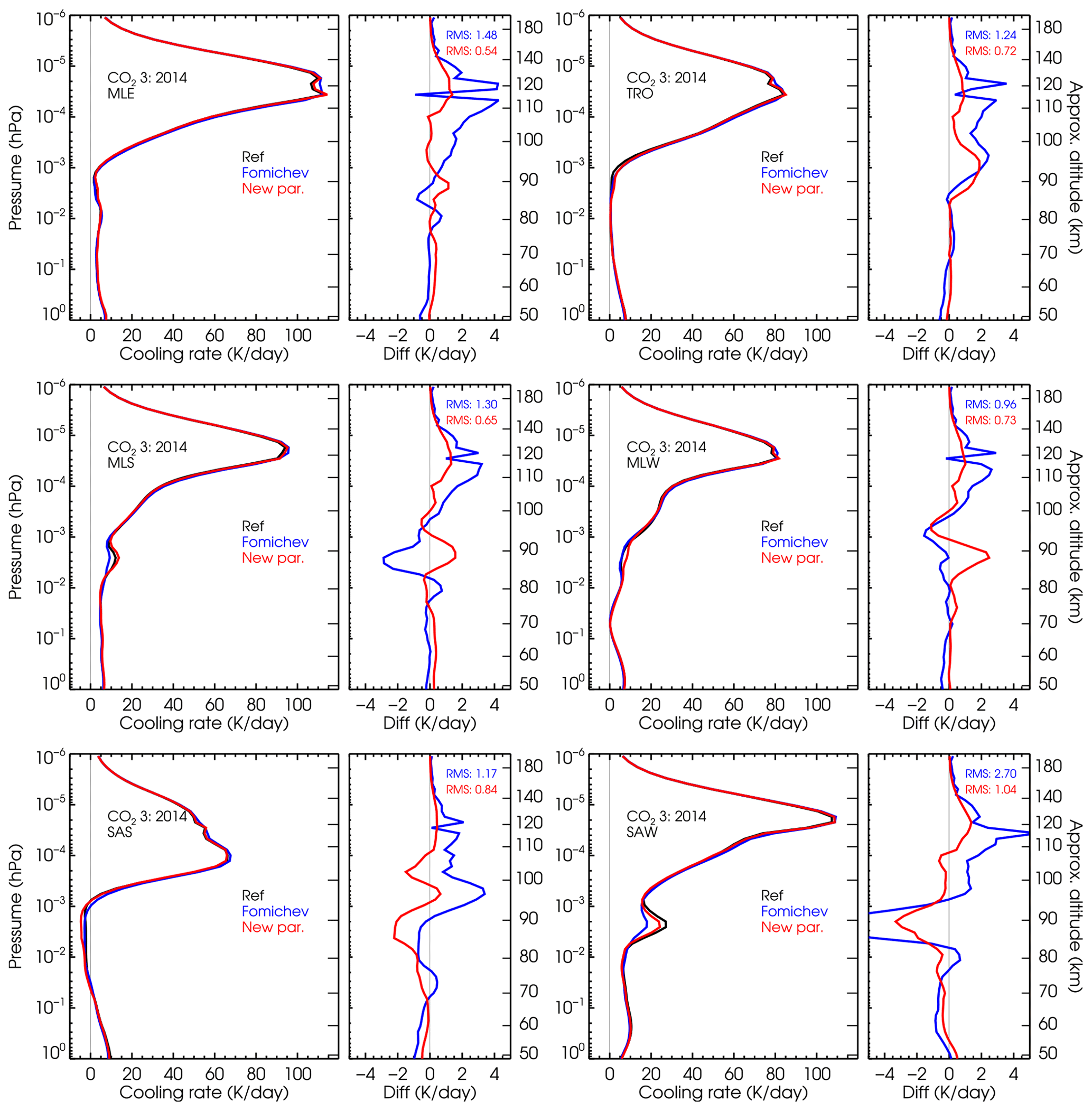
Figure 8 Comparison of the cooling rates of the current and previous parameterizations with respect to reference non-LTE cooling rates for the present-day CO₂ VMR profile no. 3 and the six p–T reference atmospheres. Note that the latter cooling rates are hardly visible in the left panels of the figures. See Figs. S9 and S10 for lower CO₂ concentrations and Figs. S11–S15 for higher CO₂ VMRs.

6.1 Accuracy of the parameterization for the reference atmospheres

In this section, we discuss the accuracy of the current parameterization for the assumed reference atmospheres. The non-LTE models used in the original (Fomichev et al., 1998) and current parameterizations are different. Hence we expect some differences caused not just by the parameterization itself, but possibly also by the different non-LTE models. Figure 8 shows the cooling rates of this parameterization compared to those of the previous parameterization and the reference ones for a contemporary CO₂ VMR profile (no. 3) and the six p–T profiles. The comparisons for the lower CO₂ profiles are shown in Figs. S9 and S10 and in Figs. S11–S15 for high CO₂ VMRs. We should clarify that, to make the comparison meaningful, the three sets of cooling rates shown here include the same updated collisional rates (Table 1). Note that these rates are different from those used in the previous parameterization (Fomichev et al., 1998). The new parameterization also supports the previous collisional rates, but it has been optimized for the new ones in Table 1. As expected, larger differences are obtained in the region between 10⁻² hPa (∼80 km) and $\mathrm{2}\times {\mathrm{10}}^{-\mathrm{5}}$ hPa (∼120 km) and are more marked for the SAS and SAW atmospheres.

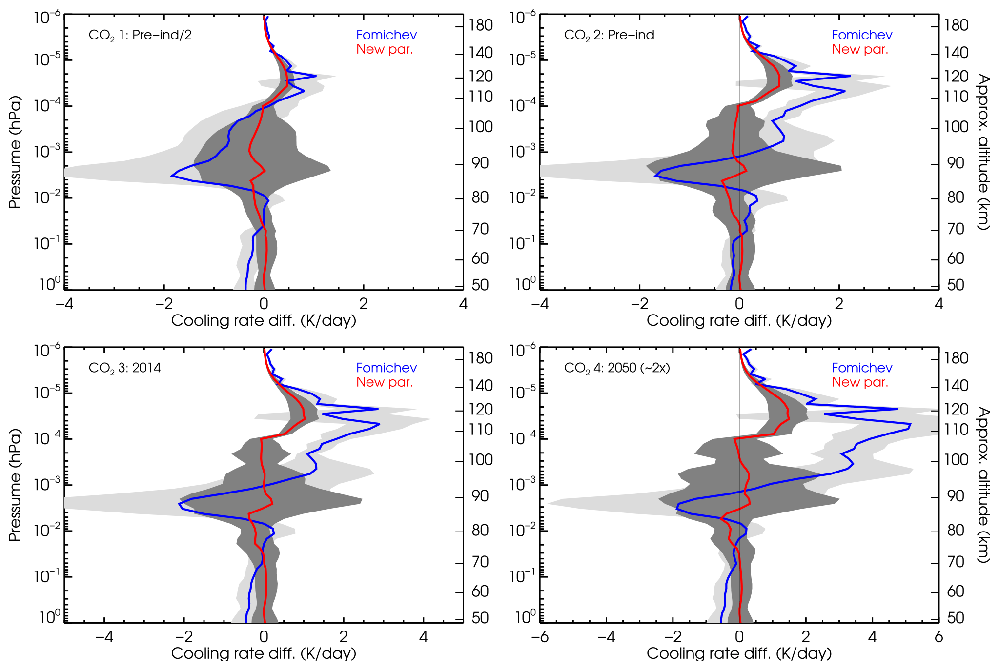
Figure 9 Mean of the cooling rate differences of the current and previous parameterizations with respect to the reference cooling rates for the four lowest CO₂ VMR profiles. The shaded areas show the standard deviation of the differences between the six p–T atmospheres. Detailed comparisons for each p–T profile are shown in Fig. 8 above and in Figs. S9, S10 and S11 in the Supplement.

The differences are more clearly illustrated in Figs. 9 and S16, where we show the mean and standard deviation of the differences for the four lowest and four highest CO₂ VMR profiles, respectively. The improvement of the new parameterization is noticeable (compare the blue and red lines). In general, the cooling rates of the current parameterization are more accurate than in the previous one for most of the regions and temperature structures. We observe that the errors (e.g. the differences with respect to the reference non-LTE cooling rates) of the new parameterization (red curves) are very small overall. They are below ∼0.5 K d⁻¹ for the current and lower CO₂ abundances (see Fig. 9). For higher CO₂ concentrations, between about 2 and 3 times the pre-industrial values, the largest errors are ∼1–2 K d⁻¹ and are located near 110–120 km (see Fig. 9 and the top-left panel in Fig. S16). The quoted values refer to the mean of the differences, although they are larger for the individual p–T atmospheres. The spread of these values is larger in the region of 10⁻² hPa (∼80 km) to 10⁻⁴ hPa (∼105 km), where the root mean square (rms) reaches values between −2 and +2 K d⁻¹ (Fig. 9).

For the very high CO₂ concentrations (4, 5 and 10 times the pre-industrial abundances), the errors are also very small, below ∼1 K d⁻¹ for most regions and conditions, except in the 107–135 km region, where we found maximum positive biases of ∼4, ∼5 and ∼16 K d⁻¹ for 4×, 5× and 10× the pre-industrial CO₂ VMR profiles (see Fig. S16). Those maximum errors are however comparable when expressed in relative terms, all about 1.2 %. The significant rms in the region of ∼80–120 km is also notable; clearly, this region is more difficult to parameterize, particularly for such a large range of CO₂ abundances.

That increase in the differences of the new parameterization with respect to the reference calculations for the very high CO₂ VMRs near 110 km seems to be related to the transition region from NLTE2 to NLTE3 (see Fig. 7). It looks like the cooling in the lower part of the NLTE3 region also requires correction by the α factor for high CO₂ VMRs. This suggests that, for higher CO₂ VMRs, the parameterization would be more accurate if this transition altitude has risen. Such a rise, however, would worsen the cooling below this boundary. This manifests the difficulty in obtaining very accurate cooling rates for a large range of CO₂ VMRs with this method.

6.2 Assessment of the cooling rates for intermediate CO₂ VMRs and for the k_O collisional rate

The aim of the parameterization is to be used for any CO₂ VMR input profile in the range of profile nos. 1 and 8 of Fig. 1b and any plausible value for the k_O rates discussed in Sect. 4.2. In this section we demonstrate that the parameterization is also very accurate for CO₂ VMRs that fall between the reference profiles used for its development and also when using different k_O values. In particular, we show results for the intermediate CO₂ VMR profile nos. 9, 10 and 11 (see Fig. 1b) and the k_O collisional rate used in the reference calculations divided by a factor of 2.

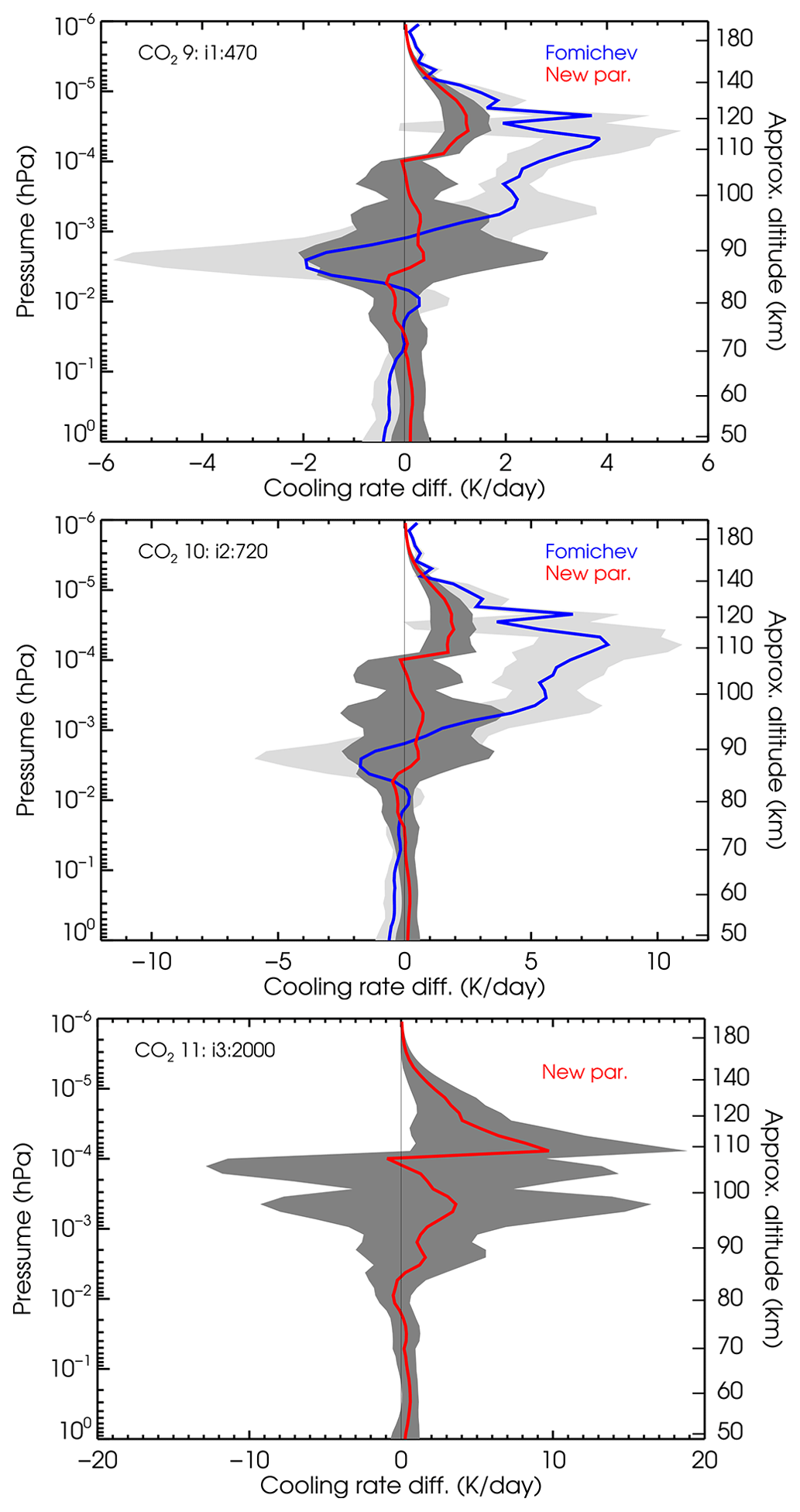
Figure 10 Mean of the cooling rate differences of the current parameterization with respect to the reference cooling rates for the intermediate CO₂ VMR profiles (nos. 9–11). The shaded areas show the difference spread (standard deviation) between the six p–T atmospheres. Note the different scales of the x axis. Detailed comparisons for each p–T profile are shown in Figs. B4, S17 and S18.

Figure B4 shows the results of the calculation for the intermediate CO₂ VMR profile no. 9, which is between the current CO₂ VMR value and that projected for 2050 (2 times the pre-industrial value). We can observe similar features in the calculations for the contemporary CO₂ VMR profile (no. 3) (see Fig. 8), although the differences are slightly larger because the CO₂ VMR profile is larger. The distinctions are more clearly seen in Fig. 10, where we show the mean and standard deviation of the differences for the six p–T profiles. The patterns in the differences, as well as their values and spreads, are very similar to those described above in Sect. 6 for the CO₂ reference profiles. The major differences appear between 105 and 135 km, reaching maximum values of 1, 2 and 9 K d⁻¹ for VMR profile nos. 9, 10 and 11, respectively. Again, we observe that the new parameterization is more accurate at practically all altitude levels. Further, the maximum values of the standard deviations of the differences for the various p–T profiles also resemble very much those discussed before, reaching maximum values of about 2 K d⁻¹, 3 K d⁻¹ and 15 K d⁻¹ for the respective CO₂ VMR profiles. Note that, although these values are larger for higher CO₂ VMRs, they are very similar when expressed in percentage.

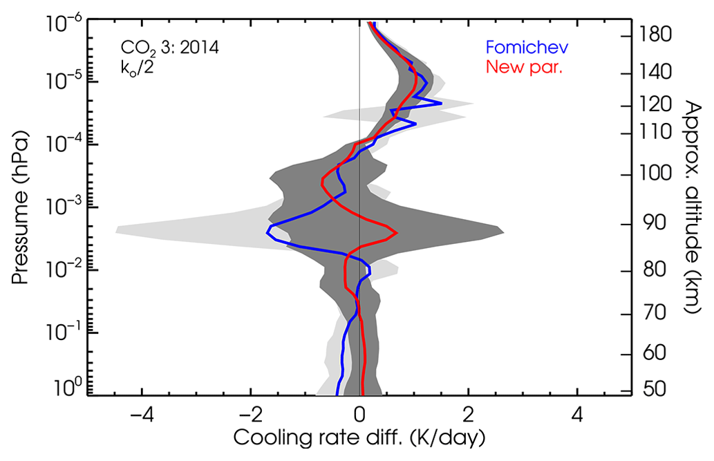
As the CO₂(v₂)–O(³P) collisional rate, k_O, is still uncertain nowadays by about a factor of 2 (see e.g. García-Comas et al., 2012) and we intend this parameterization to also be used for rates different from the nominal value, we have tested its accuracy for its lowest likely value. Figure B5 shows the results of decreasing the collisional rate k_O by a factor of 2 for CO₂ VMR profile no. 3 (current value) and the six p–T profiles. The errors incurred when using this rate are slightly larger than for the nominal rate. We see that, for the reduced rate, the differences are generally below 1 K d⁻¹ but can have values of up to 2 K d⁻¹ near 90 km for the mid-latitude summer and mid-latitude winter atmospheres and between ∼85 and 100 km for the SAS conditions. The improvement with respect to the previous parameterization is not that large for this case (see Fig. 11), only below 70 km and near 90 km, mainly caused by the significant difference incurred by the previous parameterization for the SAW atmosphere (see the bottom-right panel in Fig. B5). The smaller differences between both versions of the parameterizations for the reduced k_O are likely caused because the previous one was optimized for this reduced rate.

Figure 11 Mean of the cooling rate differences of the current parameterization with respect to the reference cooling rates for the results in Fig. B5. The shaded areas show the differences spread (standard deviation) between the six p–T atmospheres.

6.3 Performance of the parameterization

In Table 2 we list some examples of the time taken to execute the parameterization for two processors, two compilers and three atmospheric intervals. Better performance is noticeable (up to a factor of 5 faster) when using the Intel Fortran Compiler Classic (ifort) with respect to gfortran. We did not test the ifort compiler in the second processor, which suggests that the times obtained with ifort and processor no. 1 could be improved by a factor of 2.7. We did not try other more modern Fortran compilers like ifx, which could run the parameterization even faster. It is also worth mentioning that, if the atmosphere is cut in the first 50 km, the execution is about 1.76 times faster. This is because, in the lower region, where the cooling occurs under LTE conditions, the calculation involves the Curtis matrix and operations of the coefficient matrices a and b are required. Reducing this region, e.g. starting near 50 km where LTE still prevails, makes the parameterization significantly faster. Reducing the atmosphere in the upper layers, however, hardly decreases the computation time. Thus, when using a processor of type 2 with an ifort compiler for an atmosphere in the range of 50–270 km, the calculation of a cooling rate profile could be as low as 0.015 ms and still have a margin of improvement when using modern Fortran compilers like ifx.

Table 2 Performance of the parameterization.

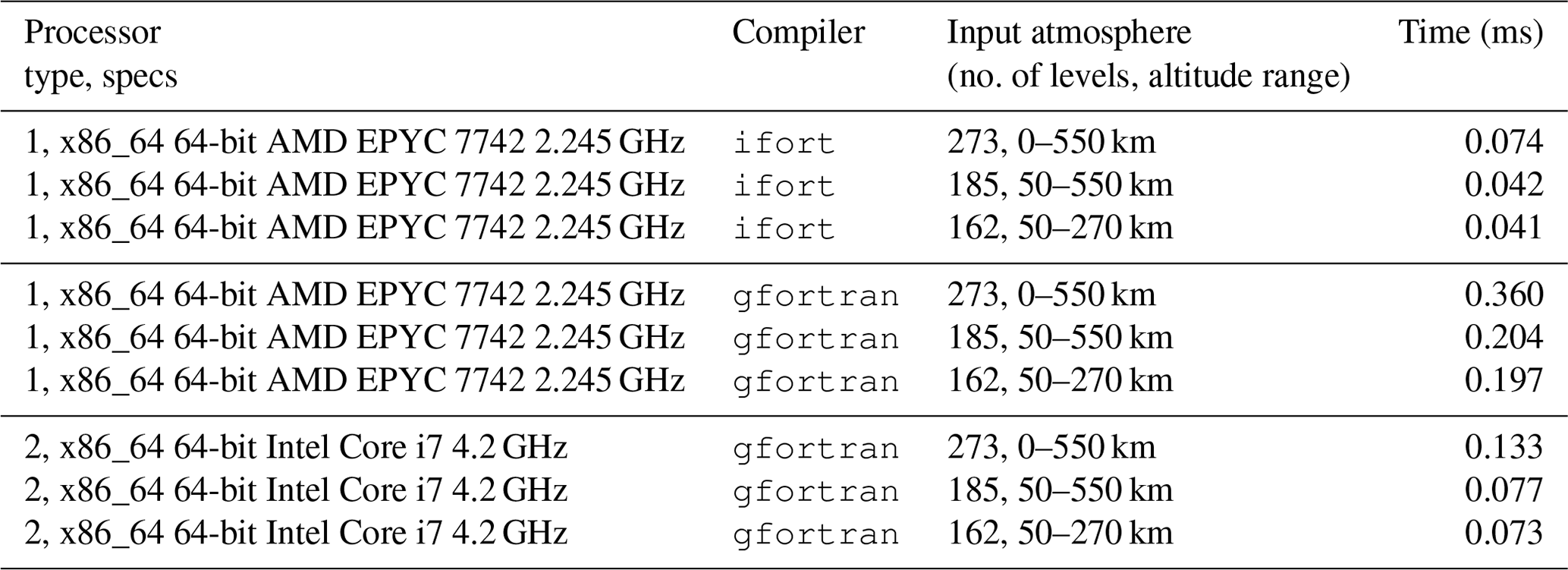
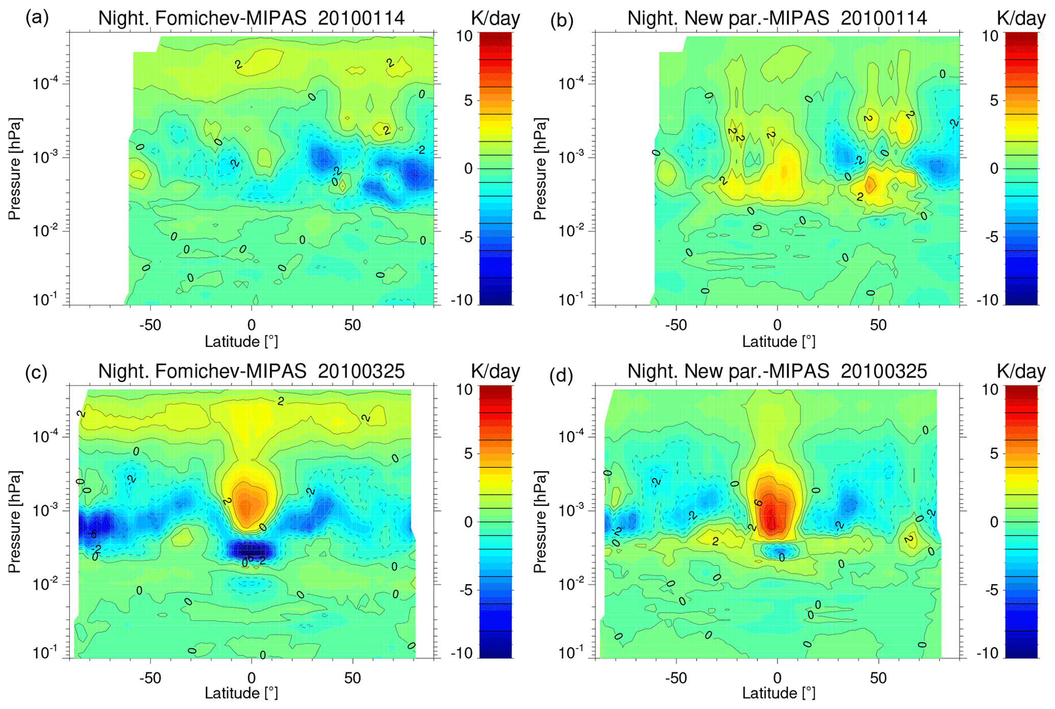
Figure 12 Zonal mean of the differences in the cooling rates of the old parameterization (a, c) and the new one (b, d) with respect to the reference cooling rates obtained for MIPAS temperatures for 14 January 2010 (solstice) and 25 March 2010 (equinox). Similar figures for 13 June 2010 (northern summer hemisphere) and 21 September 2010 (northern autumn hemisphere) are shown in Fig. B8.

7 Testing the parameterization for the MIPAS-measured temperatures

7.1 Solstice and equinox conditions

We have compared the cooling rates estimated by the parameterization with the reference ones for realistic, e.g. measured, temperature profiles that present a large variability and very variable vertical structure (see e.g. Fig. B6). Specifically, we compared them for the p–T profiles measured by the MIPAS instrument (García-Comas et al., 2023) for 5 full days of measurements (about 2500 profiles) with global latitude coverage and covering 2 d for solstice conditions (14 January and 13 June) and 2 d for equinox conditions (25 March and 21 September) for 2010. Further, we compare the results for the temperatures of 15 February 2009 when strong stratospheric warming followed by an elevated stratopause event occurred in the northern polar hemisphere (see Sect. 7.2). The comparison is carried out for the MIPAS measurements taken only under nighttime conditions, as the MIPAS non-LTE cooling rates for daytime, obtained simultaneously with the temperature inversion, also include the fraction of the 15 µm cooling which is produced by the relaxation of the solar energy absorbed by CO₂ NIR bands, which is not accounted for in this parameterization (see Sect. 9). The zonal means of the temperatures, CO₂ VMRs and O(³P) abundances for those conditions are shown in Figs. B7, S19 and S20, respectively.

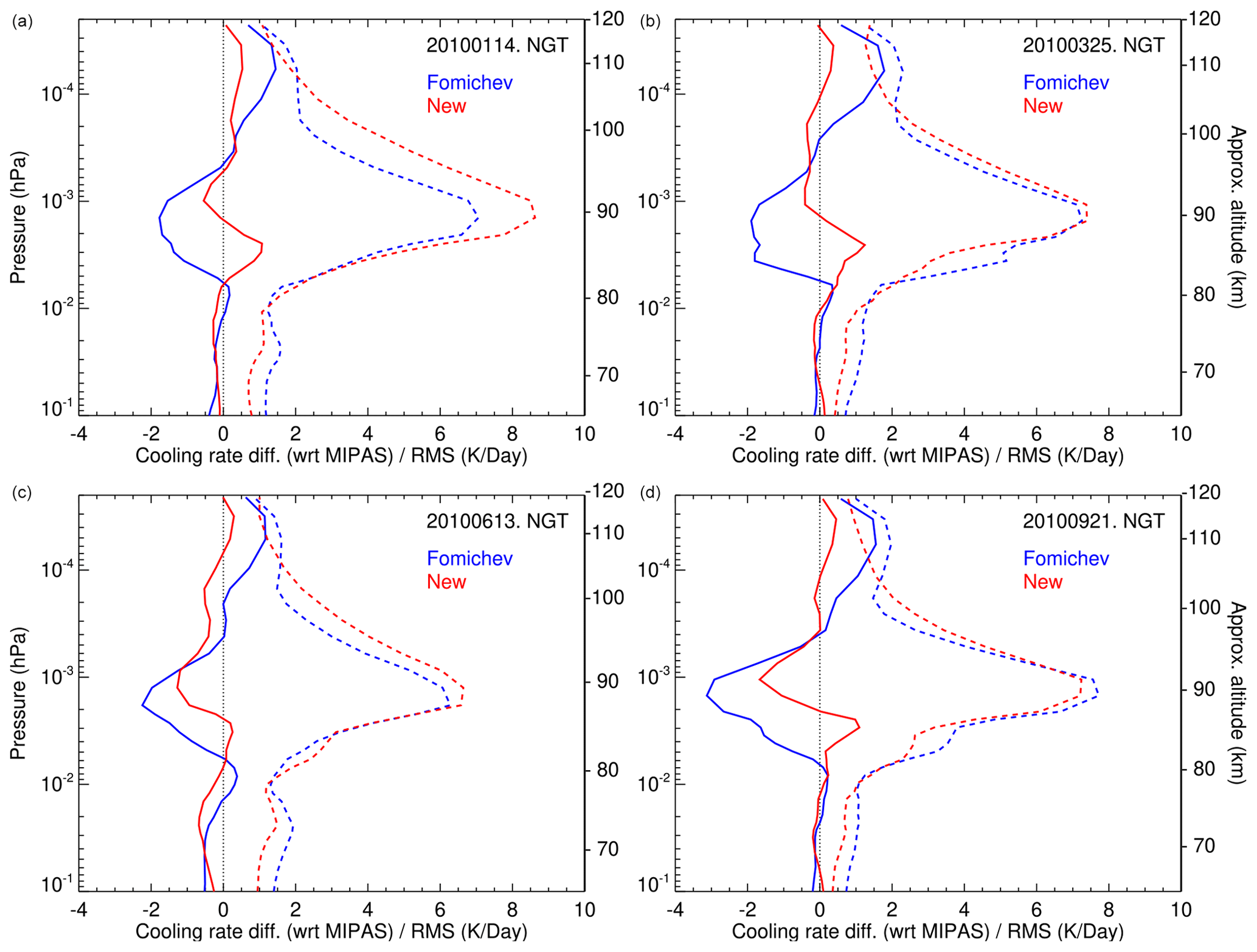
Figure 13 Mean (solid lines) and rms (dash lines) of the differences in the cooling rates of the old parameterization (blue) and the new one (red) with respect to the reference accurate cooling rates obtained for MIPAS temperatures for 14 January and 13 June 2010 (solstice, a, c) and 25 March and 21 September 2010 (equinox, b, d).

The results are presented in Fig. 12 for the zonal mean of the differences for 1 d of solstice and 1 d of equinox conditions and in Fig. 13 as the global mean difference for all latitudes for each of the 4 individual days. In general, the new parameterization is slightly more accurate. For example, the deviations of the cooling rates from the reference calculations in the altitude range of 105–115 km are larger in the old parameterization (about 2 K d⁻¹) than in the new one and are negligible in this region. Also, the differences with respect to the reference calculations are larger in the altitude range of 80–95 km for solstice conditions and at altitudes of 80–100 km for equinox conditions (see Fig. 13).

Overall, the errors in the mean profiles of the cooling rates of the new parameterization for 1 d of measurements are below 0.5 K d⁻¹, except in the region between $\mathrm{5}\times {\mathrm{10}}^{-\mathrm{3}}$ and $\mathrm{3}\times {\mathrm{10}}^{-\mathrm{4}}$ hPa (∼85–95 km), where they can reach values of 1–2 K d⁻¹. This region is the most difficult to parameterize because several bands contribute to the cooling rate, and they are very sensitive to the temperature structure of the middle atmosphere (e.g. even outside this region). Note also that this is precisely the region where the rms of the differences of the cooling rate with respect to the reference ones are largest, reaching values of up to 6 K d⁻¹ (see Fig. 13).

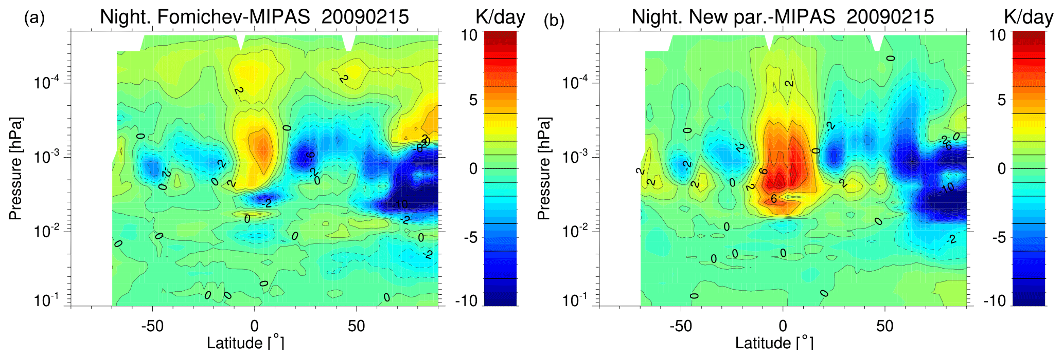
Figure 14 As in Fig. 12 but for the MIPAS temperatures taken on 15 February 2009, when a major elevated stratopause event occurred.

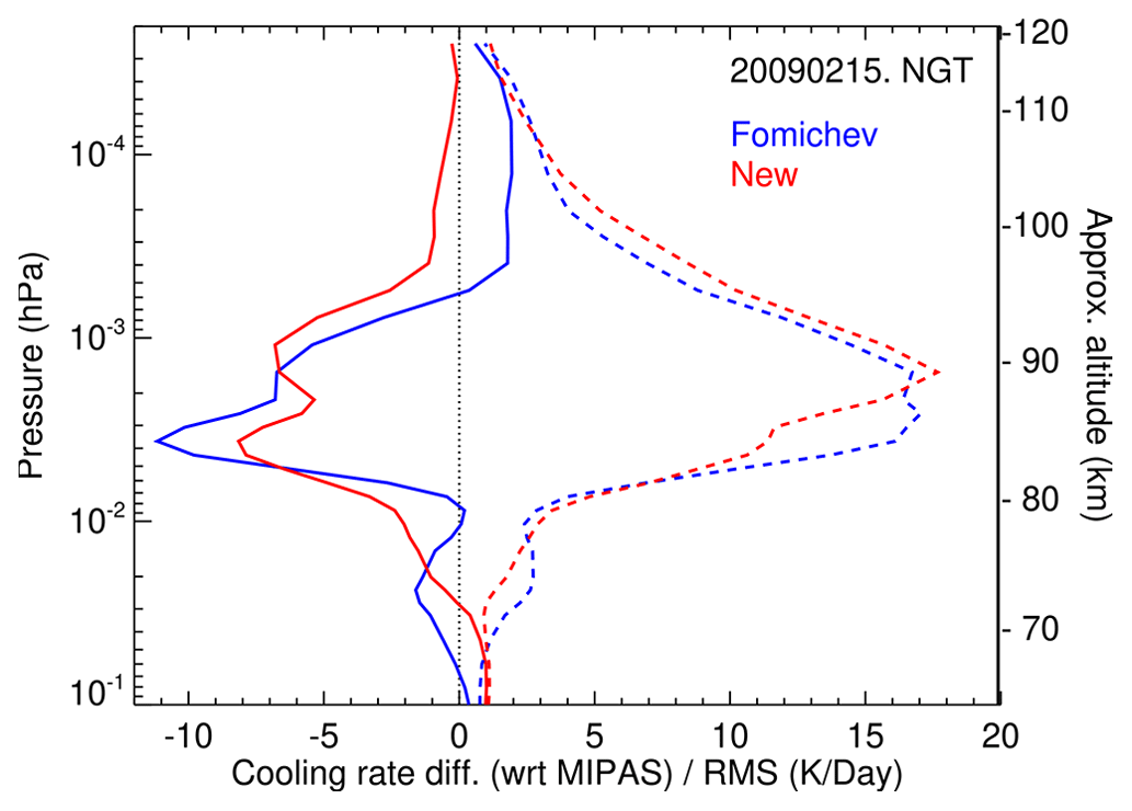
Figure 15 Mean (solid) and rms (dash) of the differences in the cooling rates of the old parameterization (in blue) and the new one (red) with respect to the reference cooling rates obtained for MIPAS temperatures for 15 February 2009 for latitudes north of 50° N.

7.2 Elevated stratopause conditions

The comparison of the cooling rates estimated by the old and new parameterizations with respect to the reference calculations for 15 February 2009, a day with a pronounced and unusual elevated stratopause event (see the zonal mean temperatures in Fig. B9), is shown in Fig. 14. Similar features to the other conditions shown above can be appreciated, except in the polar winter region. The mean of the differences and the standard deviations for all the profiles at latitudes north of 50° N are shown in Fig. 15. The differences are significantly larger than for other latitudes in the 80–95 km altitude region. Both parameterizations underestimate the cooling in that atmospheric region. The new parameterization has, however, better performance above about 80 km, but in the elevated stratopause region (80–100 km), it still underestimates the cooling by 3–7 K d⁻¹ (∼10 %).

It seems clear that part of this underestimation is caused by the fact that such atypical temperature profiles (see Sect. 3.1) were not considered in the parameterization. However, its inclusion would not solve the problem, as in the calculations of the coefficients a trade-off of the weighting of the different p–T reference atmospheres has to be chosen (see Sect. 5.1 and 5.2). Thus, it might ameliorate the inaccuracy for these elevated stratopause events but would worsen the accuracy for other general situations. This manifests the difficulty or limitation of this method in providing accurate non-LTE cooling rates for all the temperature structures (gradients) that we might find in the real atmosphere. Nevertheless, we have to keep in mind that these situations are sporadic and limited to high polar regions. Hence they should not impact significantly the accuracy of the cooling rates of this parameterization in global multiyear GCM simulations.

8 Testing the parameterization for WACCM-X high-resolution temperatures

In addition to the tests above, we have also tested the parameterizations for the temperature structure obtained with a high-resolution version of the WACCM-X model (Liu et al., 2024). This version of WACCM-X has a fine grid of 0.25° × 0.25° in latitude × longitude and a vertical resolution of 0.1 scale heights (∼0.5 km) in most of the middle and upper atmosphere, transitioning to 0.25 scale heights in the top three scale heights². With such a fine grid, the model itself can internally generate gravity waves, thus providing temperature profiles with a vertical structure very similar to that measured by high-vertical-resolution lidars of the mesosphere and lower thermosphere. Some examples of p–T profiles of the model exhibiting those vertical features and the latitudinal and longitudinal variabilities are shown in Fig. S23 of the Supplement. Further, the model spans from the surface up to nearly 600 km ($\sim \mathrm{5}\times {\mathrm{10}}^{-\mathrm{10}}$ hPa), which is ideal for testing the parameterization. In addition to the pressure–temperature profiles of the model, their O(³P), O₂ and N₂ VMR profiles have been used. A contemporary CO₂ VMR (profile no. 3) was included in these calculations.

The parameterization has been tested for a total of 225 temperature profiles. They have been selected from the model output for January conditions at four latitudes, 20, 40, 60 and 70° N of the northern winter hemisphere, and two additional latitudes, 60 and 70° S of the southern summer hemisphere. For each latitude, 36 profiles corresponding to longitudes from 0 to 360° every 10° were selected. A few p–T profiles are shown in the left column of Fig. 16, and all the profiles for latitudes 20° N, 60° N, 70° N and 70° S are shown in Fig. S23 in the Supplement. We should note that those temperature structures very much resemble those measured by lidar instruments.

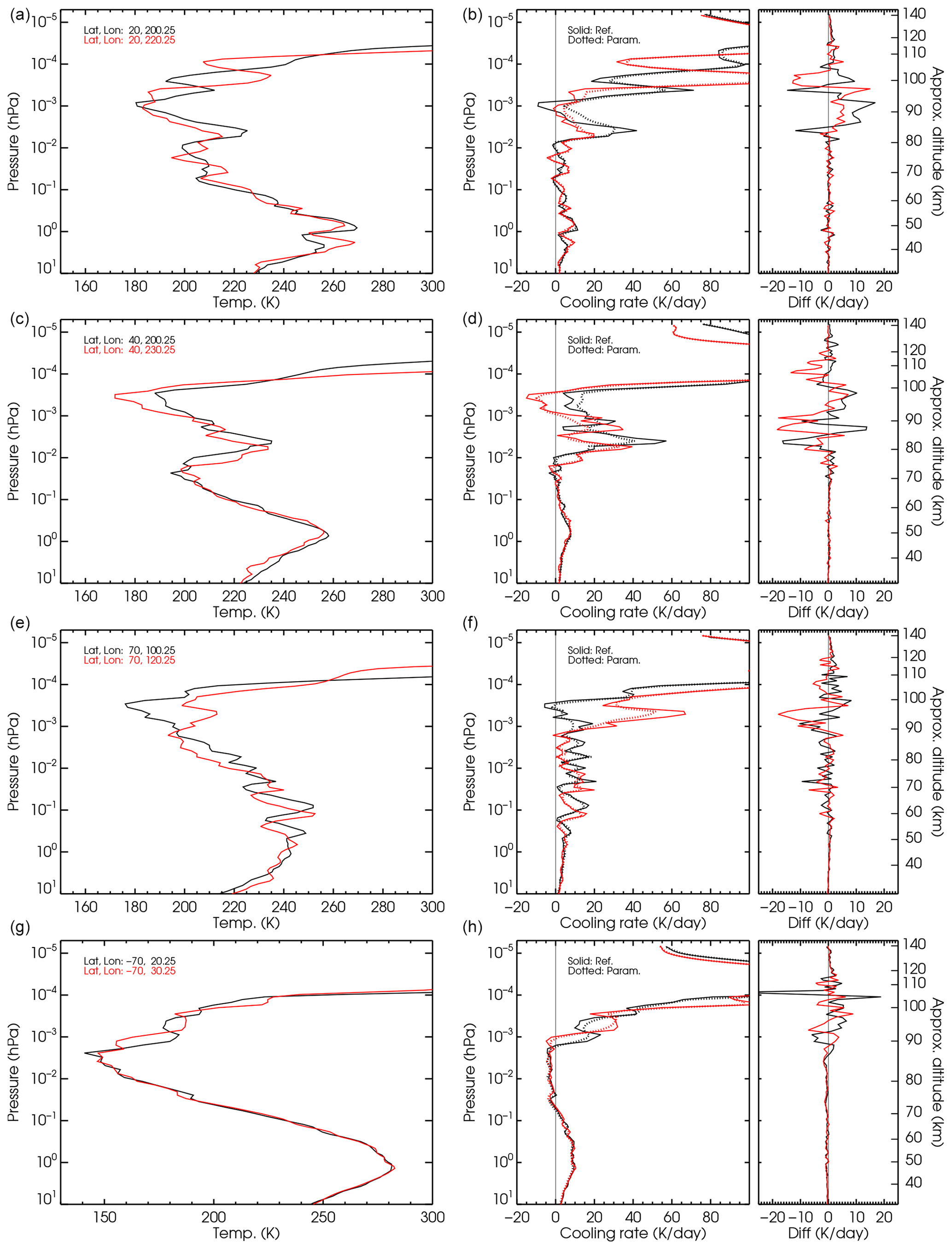
Figure 16 Comparison of cooling rates of the parameterization and the reference calculations for high-resolution WACCM-X temperature profiles. The left column shows the panels for the pressure–temperature profiles, with two profiles (black and red) in each panel. The middle column shows the reference cooling rates (solid) and the cooling rate from the parameterization (dotted) for the corresponding p–T profiles. The right column shows the differences of the parameterized cooling and the reference calculation. The different rows are results for the p–T profiles at different latitudes.

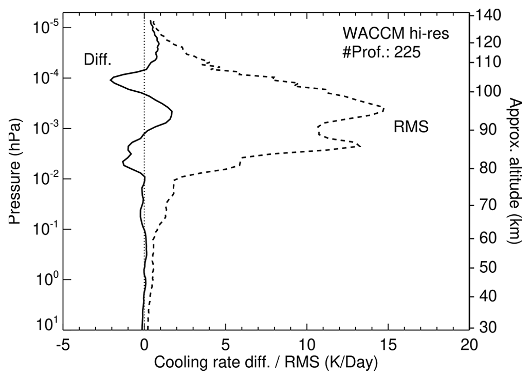
Figure 17 Mean and rms of the differences in the cooling rates of the parameterization with respect to the reference cooling rates obtained for the WACCM-X high-resolution temperature profiles.

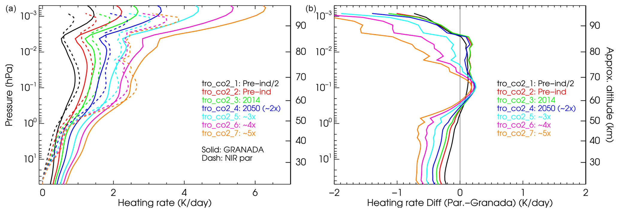
Figure 18 Solar NIR heating rates for the tropical atmosphere and a SZA of 44.5° computed by the solar NIR heating parameterization of Ogibalov and Fomichev (2003) and those obtained in the updated GRANADA model (see the text). The right panel shows the differences in the heating rates of the parameterization minus those computed in GRANADA.

The results for a few representative p–T profiles are shown in Fig. 16. A few more examples are shown in Figs. S24–S26 in the Supplement. In general, the results are very similar to those obtained for the MIPAS temperatures. The parameterization works very well below $\sim \mathrm{5}\times {\mathrm{10}}^{-\mathrm{3}}$ hPa (∼85 km), with differences generally smaller than 1–2 K d⁻¹. In the upper regions, above $\sim \mathrm{2}\times {\mathrm{10}}^{-\mathrm{4}}$ hPa (∼105 km, not fully shown in Fig. 16 because of the small scale chosen to highlight the differences in the region of larger differences), it also works very well. In this region, the cooling rate differences are slightly larger than near $\sim \mathrm{5}\times {\mathrm{10}}^{-\mathrm{3}}$ hPa (∼85 km), generally below 5 K d⁻¹, but they are much smaller in relative terms since the cooling rates at high altitudes are very large (of the order of 100–300 K d⁻¹). In the intermediate region, between $\sim \mathrm{5}\times {\mathrm{10}}^{-\mathrm{3}}$ hPa and $\sim \mathrm{2}\times {\mathrm{10}}^{-\mathrm{4}}$ hPa, the algorithm still reproduces the reference calculations rather well but not as well as in the other regions. The cooling rate differences can reach up to 10 K d⁻¹ at a few isolated levels of some individual profiles which can represent up to about 20 %. It is noticeable though that, while the differences can be significant, the profile shapes of the reference and parameterized calculations are very similar (see the middle column of Fig. 16).

To have a global perspective, we have plotted in Fig. 17 the mean of the differences for all the p–T profiles together with their rms. We see that the mean (bias) of the parameterization is very small, practically below 1.5 K d⁻¹ anywhere and below 0.5 K d⁻¹ for most of the atmospheric layers. The rms, a representative error of individual profiles, is also small at levels below $\sim \mathrm{2}\times {\mathrm{10}}^{-\mathrm{2}}$ hPa (∼80 km) with values of 1–2 K d⁻¹ (∼20 %) and above 10⁻⁴ hPa (∼105 km) with values smaller than 4 K d⁻¹ (∼2 %). In the intermediate region, between $\sim \mathrm{5}\times {\mathrm{10}}^{-\mathrm{3}}$ and $\sim \mathrm{2}\times {\mathrm{10}}^{-\mathrm{4}}$ hPa, the rms is however significant, with most values in the range of 5–12 K d⁻¹. While these values are significant in percentage at $\sim \mathrm{5}\times {\mathrm{10}}^{-\mathrm{3}}$–$\mathrm{5}\times {\mathrm{10}}^{-\mathrm{4}}$ hPa, they are very small above $\sim \mathrm{5}\times {\mathrm{10}}^{-\mathrm{4}}$ hPa.

9 Discussion: the use of this parameterization with a previous CO₂ solar NIR heating rate parameterization

Some of the GCM models use the parameterization of the CO₂ 15 µm cooling together with that of the CO₂ NIR heating of Ogibalov and Fomichev (2003). Hence, as we are updating the former for larger CO₂ abundances and as the update of the NIR heating parameterization for the large CO₂ abundances is beyond the scope of this work, we investigate whether the latter is still valid for the large CO₂ abundances. For that purpose, we compute CO₂ NIR heating rates with the parameterization of Ogibalov and Fomichev (2003) and with the GRANADA model for the large CO₂ concentrations for the six p–T reference atmospheres. We should note that the non-LTE models used in both parameterizations are different, and hence we expect some difference caused not just by the parameterization itself but also by the differences between the underlying non-LTE model in the NIR heating parameterization and GRANADA. The CO₂ NIR heating rates of GRANADA were calculated with the rate coefficients and photolysis rates described in Funke et al. (2012) but updated with those described in Jurado-Navarro et al. (2015, 2016) and also with those described below. In particular, the $J_{{\mathrm{O}}_{\mathrm{3}}}$ rate used in these calculations is ∼10 % smaller than in Jurado-Navarro et al. (2015) below 100 km and thus leads to an [O(¹D)] of ∼10 % smaller below 90 km but that is very similar near 100 km. Above ∼100 km, the $J_{{\mathrm{O}}_{\mathrm{2}}}$ coefficient used in the present calculations is about 40 % smaller than in Jurado-Navarro et al. (2015), leading to a similar reduction in [O(¹D)]. Further, we updated the following collisional rates. The rate coefficient of N₂ + O(¹D) → N₂(1) + O has been increased by a factor of 1.08, and the collisional deactivation of N₂(1) with atomic oxygen (which has an important role in the heating rates; see e.g. López-Puertas et al., 1990) has been updated from values of $\mathrm{4.5}\times {\mathrm{10}}^{-\mathrm{15}}$ $(T/\mathrm{300}{)}^{\mathrm{1.5}}$ to $\mathrm{4.3}\times {\mathrm{10}}^{-\mathrm{15}}$ $(T/\mathrm{300}{)}^{\mathrm{2.9}}$ cm³ s⁻¹.

The results of the comparison are shown in Fig. 18 for the tropical atmosphere and an intermediate solar zenith angle (SZA) of 44.5°. The region of most importance for the CO₂ NIR heating rates is that comprised between 0.1 and 0.01 hPa (Fomichev et al., 2004). In this region, the differences between the algorithm of Ogibalov and Fomichev (2003) and GRANADA are in the range of +0.2 to −0.5 K d⁻¹ for CO₂ VMRs up to 5 times the pre-industrial CO₂ profile, e.g. about 10 % to 15 %. Hence, given that they have been computed with very different non-LTE models and the significant effect that parameters like the CO₂ VMR above ∼90 km, the collisional rate between N₂(1) and O(³P), the O(³P) concentration itself and the rate of exchange of CO₂ v₃ quanta with N₂(1) have on this solar heating (see e.g. López-Puertas et al., 1990), these differences are reasonable. Hence the new CO₂ cooling rate parameterization reported here can be safely used together with the CO₂ solar NIR heating parameterization of Ogibalov and Fomichev (2003) for CO₂ VMRs up to 5 times the pre-industrial CO₂ profile.

10 Summary and conclusions

An improved and extended parameterization of the CO₂ 15 µm cooling rates of Earth's middle and upper atmosphere has been developed. It essentially follows the same method of the parameterization of Fomichev et al. (1998). The major novelty is its extended range of CO₂ abundances, ranging from CO₂ profiles with tropospheric values close to half of the pre-industrial value to 10 times that value. This extension of CO₂ profiles can still be safely applied to the parameterization of the CO₂ near-infrared heating of Ogibalov and Fomichev (2003) up to at least 5 times the pre-industrial CO₂ values and is normally combined with this cooling rate parameterization.

Other improvements or updates are as follows. They have an extended and finer vertical grid, increasing the number of levels from 8 to 83. The CO₂ line list has been updated, from HITRAN 1992 to HITRAN 2016. Although the collisional rate coefficients affecting the CO₂ v₁ and v₂ levels are input parameters for the parameterization, in this version we have used more contemporary values, e.g. as currently used in the non-LTE retrieval of temperature from CO₂ 15 µm emissions of SABER and MIPAS measurements (García-Comas et al., 2008, 2023). The rate coefficients are in general of a very similar magnitude, except for the collisional deactivation of CO₂(v₁,v₂) levels by atomic oxygen, which is now larger by approximately a factor of 2, e.g. close to its accepted upper limit. As a consequence of the larger range of CO₂ VMR profiles, the different NLTE layers for computing the cooling rates have been significantly revised. For example, it is worth mentioning that the lowermost altitude of the cooling-to-space approximation (the uppermost NLTE layer) has risen from ∼110 km to 160–170 km.

The new parameterization has been thoroughly tested against line-by-line LTE and non-LTE cooling rates for (i) the six p–T reference atmospheres; (ii) the two most important input parameters (besides temperature), the CO₂ VMR profiles and the collisional rate of CO₂(v₁,v₂) by atomic oxygen; (iii) realistic measured temperature fields of the middle atmosphere (about 2500 profiles), including an episode of strong stratospheric warming with a very elevated stratopause; and (iv) the temperature profiles (225 profiles) obtained by a high-resolution version of WACCM-X capable of generating internally gravity waves and hence with temperatures showing a large variability and pronounced vertical wave structures. Further, to illustrate the improvements, the comparisons of points (i) to (iii) have also been performed for the previous parameterization.

For the reference temperature profiles, the errors of the new parameterization (mean of the differences in the cooling rates with respect to the reference calculations for the six p–T atmospheres) are below 0.5 K d⁻¹ for the current and lower CO₂ VMRs. For higher CO₂ concentrations, between about 2 and 3 times the pre-industrial values, the largest errors are ∼1–2 K d⁻¹ and are located near 110–120 km. For the very high CO₂ concentrations (from 4 to 10 times the pre-industrial abundances) the errors are also very small, below ∼1 K d⁻¹, for most regions and conditions, except in the 107–135 km region, where the parameterization overestimates them in a few Kelvin per day (∼1.2 %). For these reference atmospheres, the new parameterization has a better performance for most of the atmospheric layers and temperature structures.

From the testing of the parameterization for realistic current temperature fields of the middle atmosphere as measured by MIPAS, we found that, in general, the new parameterization is slightly more accurate. In particular, in the 105–115 km range, the previous parameterization overestimates the cooling rate by 1.5 K d⁻¹, while the new one is very accurate. However, in the other height regions the difference is not so important. The new parameterization has a better performance in the 80–95 km altitude region. Overall, the errors in the mean profiles (bias) of the cooling rates of the new parameterization, calculated for four different atmospheric conditions with about 500 profiles in each of them, are below 0.5 K d⁻¹, except between $\mathrm{5}\times {\mathrm{10}}^{-\mathrm{3}}$ and $\mathrm{3}\times {\mathrm{10}}^{-\mathrm{4}}$ hPa (∼85–95 km), where they can reach biases of 1–2 K d⁻¹. That region is the most challenging to parameterize because several CO₂ 15 µm bands contribute to the cooling rate, and they depend very heavily on the temperature structure of the whole middle atmosphere (e.g. even outside this region). For single-temperature profiles, the cooling rate error (characterized by the rms of the difference between the reference and the parameterized cooling rates) is about 1–2 K d⁻¹ below $\mathrm{5}\times {\mathrm{10}}^{-\mathrm{3}}$ hPa (∼85 km) and above $\mathrm{2}\times {\mathrm{10}}^{-\mathrm{4}}$ hPa (∼100 km). In the intermediate region, however, it is significant, between 2 and 7 K d⁻¹. We have further tested the parameterization against very rare and demanding situations, such as the temperature structures of stratospheric warming events with an elevated stratopause. In these situations, however, the parameterization underestimates the cooling rates by 3–7 K d⁻¹ (∼10 %) at altitudes of 80–100 km, and the individual cooling rates show a significant rms (5–15 K d⁻¹).

In addition, we have tested the parameterization for the temperature structure obtained by a high-resolution version of WACCM-X, with the temperatures showing a large variability and pronounced vertical wave structure. The mean (bias) error of the parameterization is very small, smaller than 0.5 K d⁻¹ for most atmospheric layers, and below 1.5 K d⁻¹ for almost any altitude from the surface up to 200 km. The rms of the differences in the cooling rates from the parameterization and the reference model is similar to that obtained for MIPAS temperatures, with values of 1–2 K d⁻¹ (∼20 %) below $\sim \mathrm{2}\times {\mathrm{10}}^{-\mathrm{2}}$ hPa (∼80 km) and smaller than 4 K d⁻¹ (∼2 %) above 10⁻⁴ hPa (∼105 km). In the intermediate region, between $\sim \mathrm{5}\times {\mathrm{10}}^{-\mathrm{3}}$ and $\sim \mathrm{2}\times {\mathrm{10}}^{-\mathrm{4}}$ hPa, they are slightly larger than for MIPAS, with values in the range of 5–12 K d⁻¹. These values, while they are significant in relative terms at $\sim \mathrm{5}\times {\mathrm{10}}^{-\mathrm{3}}$–$\mathrm{5}\times {\mathrm{10}}^{-\mathrm{4}}$ hPa, are very small in percentage above $\sim \mathrm{5}\times {\mathrm{10}}^{-\mathrm{4}}$ hPa.

As has been shown, this parameterization has some limitations (see Sects. 6, 7.2 and 8). In order to be able to apply specific approximations for the cooling rates, it has been designed for fixed atmospheric regions where specific radiative transfer regimes prevail. Thus, its extension to a very large range of CO₂ abundances inevitably causes a loss of accuracy for extreme cases in specific atmospheric layers. A possible solution for future updates could be to use different extensions of the non-LTE regions (i.e. Fig. 7) for different abundances of CO₂. Likewise, this parameterization (like the original one) was devised for use in GCMs, i.e. to produce accurate cooling rates globally, e.g. when considering all expected temperature profiles covering the different latitudinal and seasonal conditions. Thus, the ability of the parameterization to compute accurate cooling rates for individual temperature profiles with large temperature gradients in the $\mathrm{5}\times {\mathrm{10}}^{-\mathrm{3}}$ hPa (∼85 km) to $\mathrm{3}\times {\mathrm{10}}^{-\mathrm{4}}$ hPa (∼95 km) region is limited. On the contrary, it is extremely fast. The routine takes only 15 µs of CPU time to calculate a profile in the range of 50 to 270 km on a machine with an Intel Core i7 4.2 GHz processor when compiled with ifort. This is more than 6600 times faster than the best option of the NLTE15μmCool-E v1.0 routine recently reported by Kutepov and Feofilov (2023). To conclude, parameterizations overcoming those limitations but retaining that speed are highly desirable for development in the future.

Appendix A: Notes and recommendations for using the parameterization

The routine source code is written in Fortran 90 and is available at https://doi.org/10.5281/zenodo.10849970 (López-Puertas et al., 2024). It has been devised for implementation in general circulation models, although it can also be used for other purposes, e.g. to compute the CO₂ 15 µm cooling rate for a given reference atmosphere.

The code is organized in a library (in the directory source/modules/) that can be included in a more complex GCM model. The subroutine to be called is CO2_NLTE_COOL inside module file co2cool.f90.

The following inputs are required (in order) by CO2_NLTE_COOL.

• Atmospheric profiles as a function of pressure for temperature and four VMRs of CO₂, O, O₂ and N₂

• lev0: the index of the given pressures so that p(lev0) is the maximum pressure level (lower boundary) to be considered for calculating the heating rate. Heating rates will be calculated from that pressure up to the minimum pressure specified in the pressure array. For example, if p is given in the range of 10³ to 10⁻⁶ hPa (or 10⁻⁶ to 10³ hPa) and p(lev0) = 1 hPa, the heating rate will be calculated in the range of 1 to 10⁻⁶ hPa.

• surf_temp: surface temperature – if set to a negative value, the temperature of the maximum pressure level will be used.

• hr: heating rate. This is an input–output array with the same dimension of pressure. It will only be calculated at pressures in the range of p(lev0) (the maximum pressure considered) to the minimum specified pressure (minimum(pressure)). Note that throughout this paper we have used the term “cooling rates”, e.g. the hr values with changed signs.

• The values are the temperature (K), pressure (hPa), VMRs (mol mol⁻¹, not ppm) and heating rate (K d⁻¹).

• Input profiles can run either from the ground to the top of the atmosphere (decreasing pressures) or reverse (top to ground with increasing pressures). The pressure grid can be irregular.

• Important notes:
  calculations in the LTE region.

  1. Pressure levels should include the surface pressure (near 10³ hPa), even if the 15 µm cooling is to be calculated only at lower pressure levels (higher altitudes), i.e. p(lev0) ≪ 10³ hPa.

  2. If 15 µm cooling is only calculated in the non-LTE regime, it is recommended to set up the lower boundary, p(lev0), close to the limit of the LTE–non-LTE transition, e.g. near 1 hPa. In this way, more time-consuming calculations in the LTE region will be avoided.

The output is expressed as the heating rate (K d⁻¹) on the given input grid in the range of p(lev0) to the minimum specified pressure.

To compile the routine, follow these steps.

• Edit Makefile and change the Fortran compiler to your preferred choice (e.g. gfortran or ifort).

• From this folder, run make.

The compilation produces a test program run_cool (see below) and a module library file lib/libco2_cool.a.

A test program, source/main.f90, is also provided to test the parameterization on individual profiles. Its input file input.dat has a fixed format. Do not change the number of commented lines.

• First input at line 9: n_lev, lev0 and T_surf

• Start from line 12.

• Six atmospheric profiles are read (n_lev rows are expected).

The output heating rates are written in the output.dat file. To test main.f90, two input–output files are provided: input_test.dat and input_test2.dat with their corresponding output_test.dat and output_test2.dat output files. The first computes the heating in the full pressure range provided, the second only at pressures smaller than ∼1 hPa. To test the routine, follow these steps.

• cp input_test.dat input.dat

• ./run_cool

• Check that the results in output.dat are consistent with output_test.dat.

• The same procedure can be done for test 2.

The routine is supplied with the collisional rates described in this paper (see Table 1). Nevertheless, they can be changed by the user. They are prescribed in the constants.f90 module.

• The rates are defined in the form $z=a\sqrt{T}+b\exp (-g{T}^{-\mathrm{1}/\mathrm{3}})$.

The coefficients are specified as follows.

• for CO₂–O: a_zo, b_zo, g_zo (default: $\mathrm{3.5}\times {\mathrm{10}}^{-\mathrm{13}}$, $\mathrm{2.32}\times {\mathrm{10}}^{-\mathrm{9}}$, 76.75)

• for CO₂–O₂: a_zo2, b_zo2, g_zo2 (default: $\mathrm{7.0}\times {\mathrm{10}}^{-\mathrm{17}}$, $\mathrm{1.0}\times {\mathrm{10}}^{-\mathrm{9}}$, 83.8)

• for CO₂–N₂: a_zn2, b_zn2, g_zn2 (default: $\mathrm{7.0}\times {\mathrm{10}}^{-\mathrm{17}}$, $\mathrm{6.7}\times {\mathrm{10}}^{-\mathrm{10}}$, 83.8)

The most likely rate to be changed is k_O, probably by using smaller values. We tested a collisional k_O rate 2 times smaller than used in the development of the parameterization and found that its accuracy did not change significantly (see Sect. 6.2).

Although the parameterization is specifically developed for the CO₂ 15 µm non-LTE region, it also works for the LTE region, but the user should be cautious that other important cooling rates in the LTE region, such as those of O₃ and H₂O, are not included. We recommend that GCM users utilize their radiation scheme in the LTE region and this parameterization in the non-LTE region (e.g. above ∼50 or 60 km).

Boundaries of the parameterization. About the lower boundary (maximum pressure), see the notes above. About the upper boundary (minimum pressure), there is in principle no limitation, but we recommend setting it as high as the upper lid of your model. There is a large number of GC and CC models with an upper lid at $\sim {\mathrm{10}}^{-\mathrm{2}}$ hPa (or ∼80 km). This parameterization can be used for such models to compute the CO₂ non-LTE cooling rates between ∼50 and ∼80 km. We note that, under these circumstances, the cooling rates near the upper lid might not be accurate, as the contribution of the layers above the upper lid is not considered. This, however, is not a limitation of the parameterization itself but an intrinsic limitation of this kind of model. There is no restriction either on the upper limit of the upper boundary, provided it is physically meaningful. That is, it can be placed at altitudes as high as 500 km or higher.

Appendix B: Additional figures

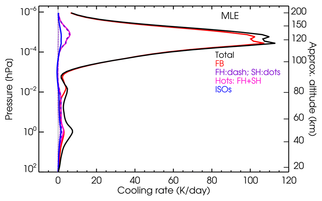
Figure B1 Contributions of the different CO₂ bands to the cooling rates for the MLE p–T atmosphere. That is, like the left panel of Fig. 4 but for the entire altitude range.

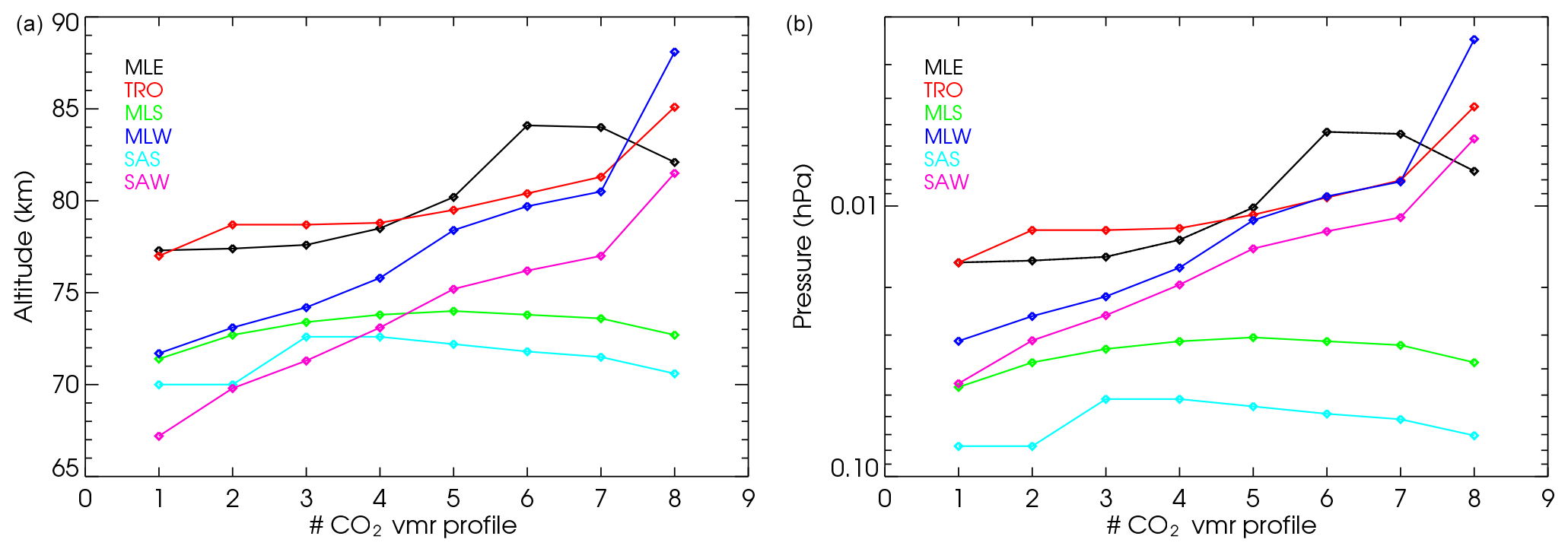
Figure B2 Altitude (a) and pressure level (b) of the deviation (≥5 %) of the non-LTE cooling rates from LTE values for the six p–T reference atmospheres and the eight CO₂ VMR profiles (see Fig. 1b): no. 1, half of the pre-industrial; no. 2, the pre-industrial; no. 3, present day; no. 4, ∼2×pre-industrial; no. 5, $\sim \mathrm{3}\times$ pre-industrial; no. 6, $\sim \mathrm{4}\times$ pre-industrial; no. 7, $\sim \mathrm{5}\times$ pre-industrial; and no. 8, $\sim \mathrm{10}\times$ pre-industrial.

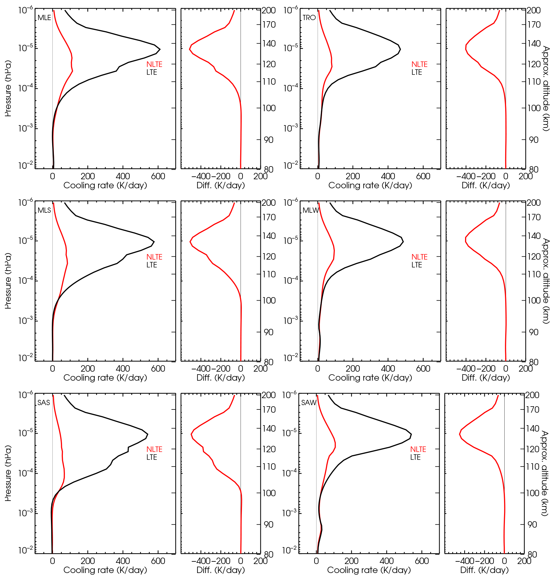
Figure B3 Non-LTE–LTE cooling rate differences for the six p–T reference atmospheres and the present-day CO₂ VMR profile no. 3 (as in Fig. 5) but including the thermosphere.

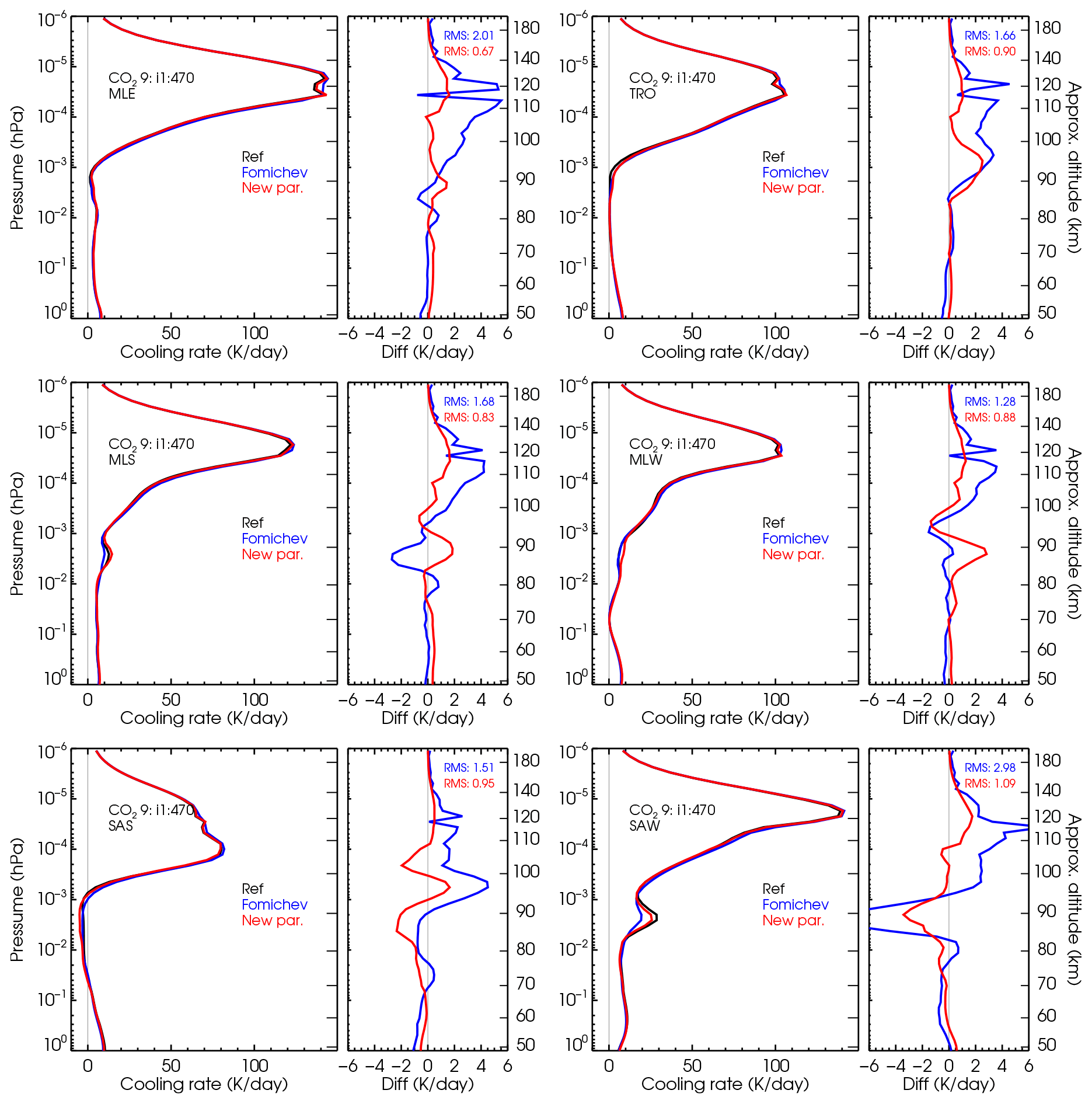
Figure B4 Comparison of the cooling rates of the current and previous parameterizations with respect to accurate cooling rates for the intermediate CO₂ VMR profile no. 9 (see Fig. 1b) and the six p–T reference atmospheres.

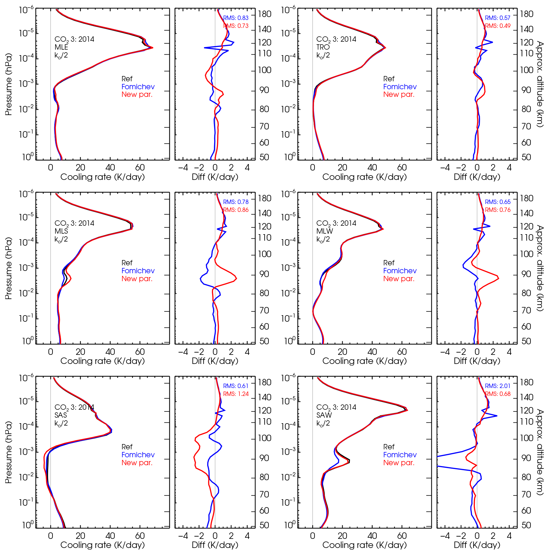
Figure B5 Testing the effect of the CO₂(v₂)–O(³P) collisional rate on the parameterization. Comparison of the cooling rates of the current and previous parameterizations with respect to the reference cooling rates for the present-day CO₂ VMR abundance (profile no. 3; see Fig. 1b) and the six p–T reference atmospheres when reducing the nominal collisional rate in Table 1 by a factor of 2.

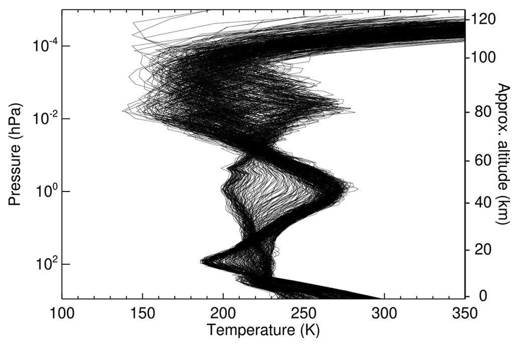
Figure B6 An example of the MIPAS nighttime temperature profiles (15 February 2009) used for verifying the parameterization accuracy. Note the large variability of the temperature profiles.

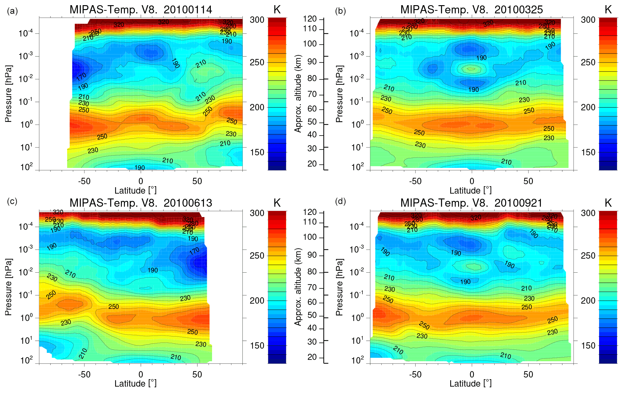
Figure B7 MIPAS zonal mean nighttime temperatures for 14 January 2010 (northern winter hemisphere, a), 25 March 2010 (northern spring hemisphere, b), 13 June 2010 (northern summer hemisphere, c) and 21 September 2010 (northern autumn hemisphere, d).

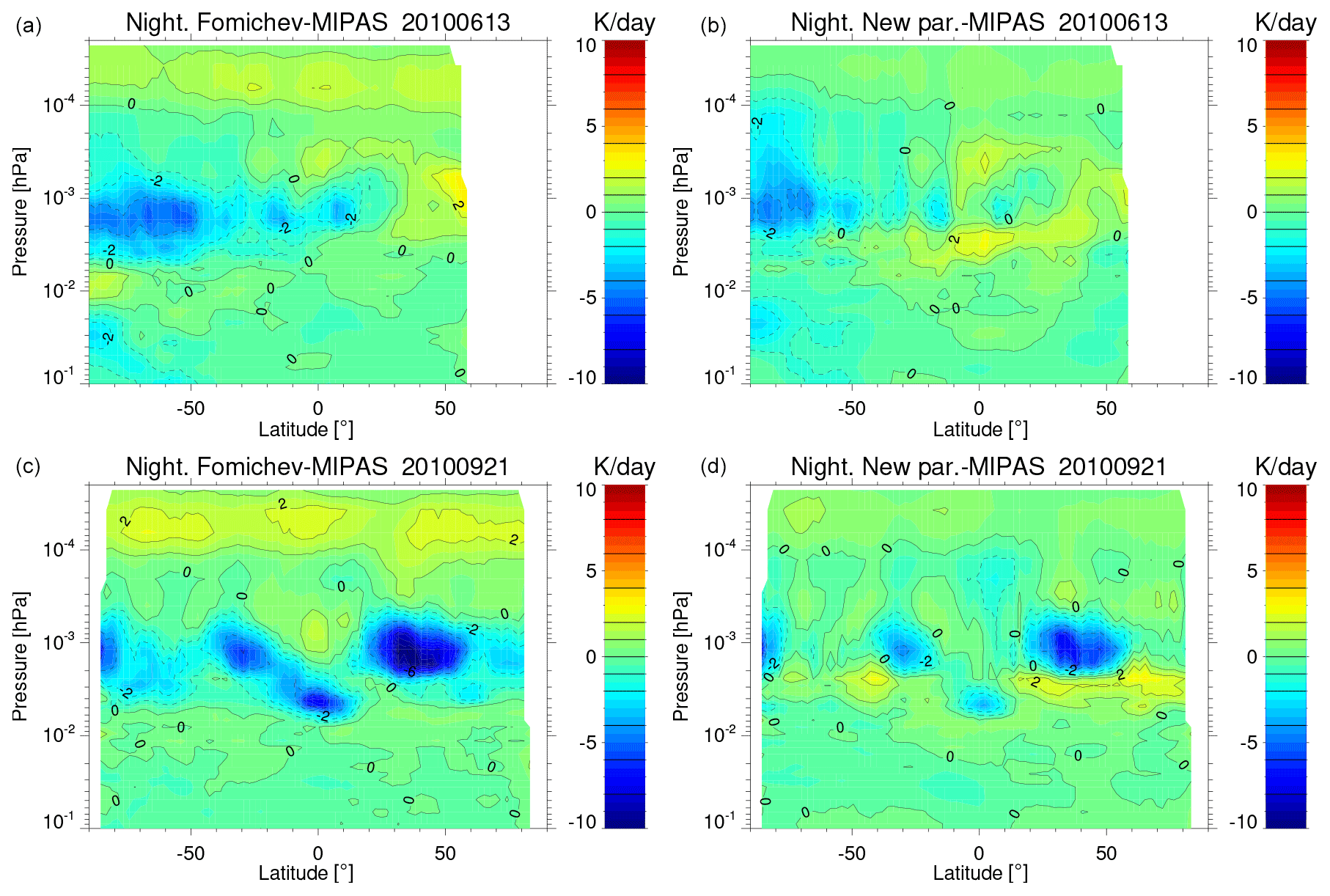
Figure B8 Zonal mean of the differences in the cooling rates of the old parameterization (a, c) and the new one (b, d) with respect to the reference cooling rates obtained for MIPAS temperatures for 13 June 2010 (northern summer hemisphere) and 21 September 2010 (northern autumn hemisphere).

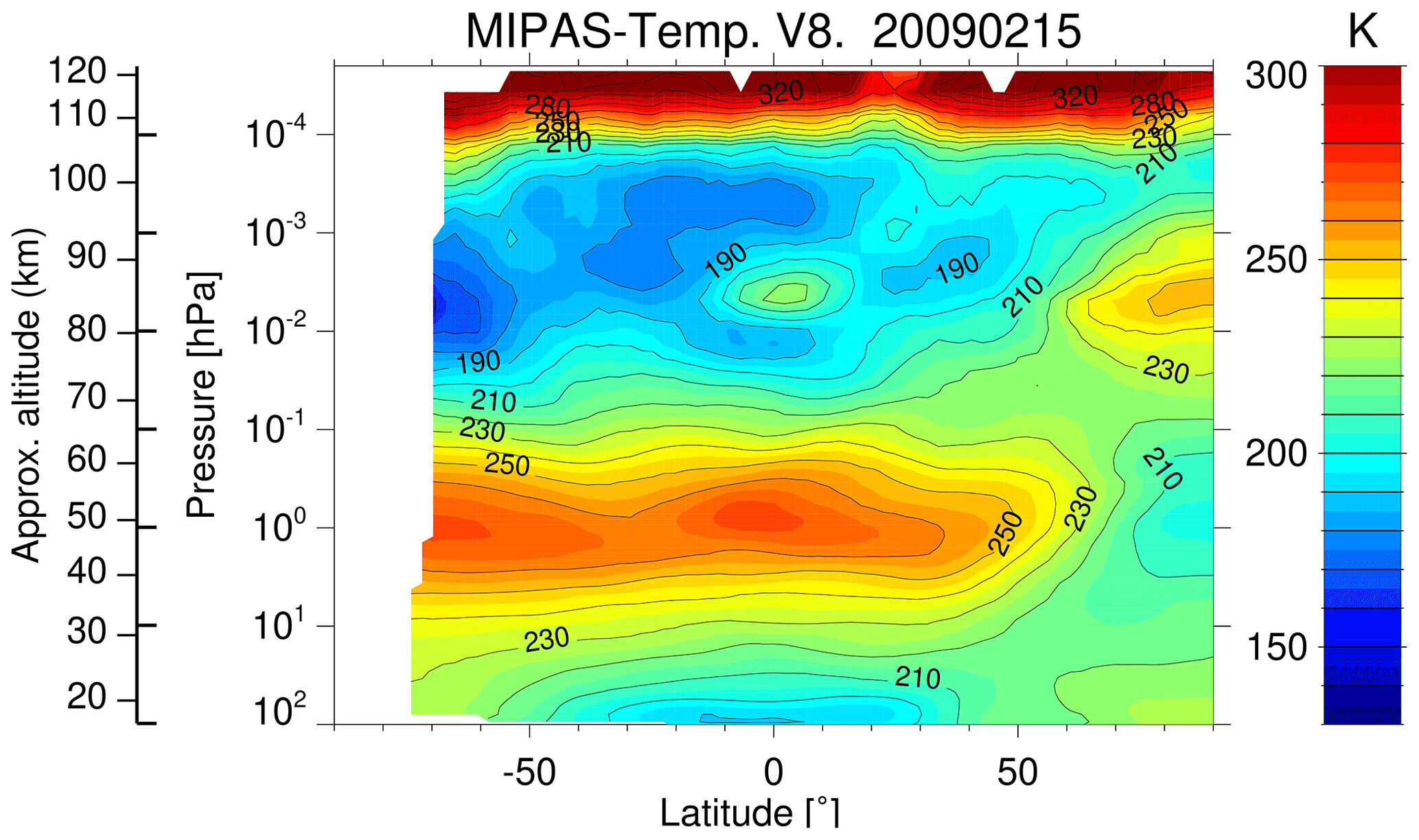
Figure B9 The MIPAS nighttime temperature zonal mean for 15 February 2009 (see also Fig. B6), used for verifying the parameterization accuracy under stratospheric sudden warming and elevated stratopause conditions. Note the high-altitude location of the stratopause in the northern polar region.