MELPF version 1: Modeling Error Learning based Post-Processor Framework for Hydrologic Models Accuracy Improvement

This paper studies how to improve the accuracy of hydrologic models using machine-learning models as post-processors and presents possibilities to reduce the workload to create an accurate hydrologic model by removing the calibration step. It is often challenging to develop an accurate hydrologic model due to the time-consuming model calibration procedure and the nonstationarity of hydrologic data. Our findings show that the errors of hydrologic models are correlated with model inputs. Thus motivated, we propose a modeling-error-learning-based post-processor framework by leveraging this correlation to improve the accuracy of a hydrologic model. The key idea is to predict the differences (errors) between the observed values and the hydrologic model predictions by using machine-learning techniques. To tackle the nonstationarity issue of hydrologic data, a moving-window-based machine-learning approach is proposed to enhance the machine-learning error predictions by identifying the local stationarity of the data using a stationarity measure developed based on the Hilbert–Huang transform. Two hydrologic models, the Precipitation–Runoff Modeling System (PRMS) and the Hydrologic Modeling System (HEC-HMS), are used to evaluate the proposed framework. Two case studies are provided to exhibit the improved performance over the original model using multiple statistical metrics.

1 Introduction

1.1 Motivation

Hydrologic models are commonly used to simulate environmental systems, which help us to understand water systems and their responses to external stresses. They are also widely used in scientific research for physical process studies and environmental management for decision support and policy-making (Environmental Protection Agency, 2017). One of the most important criteria for model performance evaluations is prediction accuracy. A reliable model is able to capture the hydrologic features with robust and stable predictions. However, it is challenging to develop a reliable hydrologic model with low biases and variances. In this paper, we aim to develop a post-processor framework, named MELPF, which is short for Modeling Error Learning based Post-Processor Framework, to improve the reliability of hydrologic models.

Hydrologic models are typical environmental models for hydrologic process studies and water resource evaluations. Among all types of hydrologic models, physically based parameter-distributed hydrologic models have become increasingly prevalent as they are able to capture detailed features within hydrologic systems. However, in regions with high hydrologic heterogeneities, a large number of parameters are required to represent both temporal and spatial variation. This requires a large amount of computational resources, which substantially increases difficulties in model development, data assimilation, and model calibration (Ye et al., 2014). The resulting high cost of computation makes it challenging to implement data assimilation techniques such as ensemble Kalman filters (Slater and Clark, 2006; Liu et al., 2016) or use an optimization method such as shuffled complex evolution (Duan et al., 1992, 1994). On the other hand, the post-processing methodologies dealing with model results can potentially mitigate such computation requirements and improve the performance (Ye et al., 2014). Therefore, the post-processor approach is studied and used in this paper. By studying many hydrologic scenarios, we observe that hydrologic model errors often follow some patterns that are highly correlated with model inputs (see Fig. 3). Such patterns can be learned via machine learning (see Sect. 2) and applied in predictions. Thus motivated, we propose that MELPF can learn the modeling error to enhance the prediction accuracy.

Despite the potential improvement brought by machine-learning techniques, it is worth noting that pure machine-learning techniques cannot completely replace hydrologic models. When we compare the performance of the environmental model and machine-learning methods, it turns out that the accuracy of the Precipitation–Runoff Modeling System (PRMS) (Leavesley et al., 1983; Markstrom et al., 2005, 2015) is much higher than that of commonly used machine-learning techniques (e.g., random forest tree, Breiman, 2001; gradient-boosted tree, Hastie et al., 2009). Compared to hydrologic models developed using domain knowledge, pure machine-learning models with limited training data cannot accurately characterize all the features of the underlying physical process. Nevertheless, based on hydrologic simulation, machine-learning approaches are able to further enhance hydrologic model results by predicting the original modeling errors via learning the relationships between model inputs and output simulation results. In the hydrologic modeling results, the term “simulations” is widely used for both concepts of historical record replication and future prediction.

1.2 Major contributions

In this paper, we develop a modeling-error-learning-based post-processor framework to enhance the prediction accuracy of hydrologic models. Based on the results in Sect. 3, the proposed MELPF can ease the parameter tuning processes and achieve accurate predictions. The key idea is to leverage the correlation between the hydrologic model inputs and model output errors. There are two main challenges of building the proposed framework: (1) how to improve the efficiency and accuracy in a hydrologic model in terms of model simulation and development and (2) how to deal with the nonstationary hydrologic data. To solve the first challenge, we propose a machine-learning-based post-processor, which can capture and characterize model errors to improve hydrologic model predictions. This can help to avoid the misleading effects of irrelevant model inputs. Also, we propose cleaning and normalizing the data, which enables a better characterization of the correlation. To solve the second challenge, we propose a window size selection method, which identifies local stationary regions of the data by using a stationarity measure based on the Hilbert–Huang transform (HHT; Huang et al., 1998). The key idea is to first find all possible window sizes by using data autocorrelation and then select the best window size, which contains the most stationary data. The stationarity measure is proposed to calculate the data stationarity within a window. The two major contributions of this paper are summarized as follows.

• MELPF is developed to improve the prediction accuracy and flexibility of hydrologic models. One common issue of existing hydrologic simulation studies is that the development of hydrologic models, in terms of calibration processes, often requires long research time cycles but ends up with barely satisfied model accuracy. To tackle these challenges, the proposed MELPF can significantly simplify the parameter tuning processes by learning and calibrating the modeling error using machine-learning techniques. Moreover, the proposed MELPF can use different machine-learning methods for different scenarios to obtain the best results, and the model parameters can be dynamically updated using the latest data. Our experiment results in Sect. 3 show that our method can significantly improve prediction accuracy compared with the simulation results of existing hydrologic models.

• A moving-window-based machine-learning approach is proposed, which can enhance the performance of the machine-learning technique when dealing with nonstationary hydrologic data. We observe that the distribution of hydrologic data changes over time and the data exhibit seasonality (see Fig. 2). The proposed moving-window-based machine-learning approach can characterize the time-varying relationship between the model inputs and model output errors. The key step is to choose a suitable window size within which the data are stationary, as most machine-learning techniques are designed for stationary data. By leveraging recent advances in the field of nonlinear and nonstationary time series analysis, particularly HHT, we propose the degree of stationarity to measure the local stationarity of the data. Based on the degree of stationarity and the autocorrelation, we propose a window size selection method to optimize the performance of the machine-learning techniques.

The proposed MELPF has been evaluated on the basis of different hydrologic models. MELPF can improve the accuracy of the original hydrologic models, and the window selection method can find the data pattern and select a suitable window size. Moreover, we find that the accuracy of an uncalibrated hydrologic model is as good as the calibrated one by using the proposed framework, which indicates that the proposed framework can replace the complicated “calibration” step in the traditional hydrologic model development workflow. Section 3 introduces more details of the case studies.

1.3 Related work

An appropriate window size is very important for training a machine-learning model to deal with nonstationary time series data. Most of the existing work on window size selection is based on concept drifts and distribution changes. There are some methods that perform well but can only be applied to a certain machine-learning method, such as Klinkenberg and Joachims (2000) and Bifet Figuerol and Gavaldà Mestre (2009). Bifet Figuerol and Gavaldà Mestre (2009) proposed a concept-drift-based method to dynamically adapt the window size for a Hoeffding tree (Domingos and Hulten, 2000). To solve the limitation, some methods are proposed that can be applied to different machine-learning techniques by using statistical techniques to monitor the concept drifts. In Klinkenberg and Renz (1998), Lanquillon (2001), and Bouchachia (2011), statistical process control (SPC; Oakland, 2007) is leveraged to monitor the data change rate by using the error rate. If the error rate change is larger than a threshold, it means the data are not stable, and then the window size should be changed. These methods need to assume that the error rate follows a certain distribution, and then calculate the threshold by using the error confidence interval. Similarly, in Gama et al. (2004) and Bifet and Gavalda (2007), window selection methods are proposed based on the concept of context with the stationary distribution. The proposed methods require the dataset inside a window to follow a certain distribution, and then calculate the confidence interval by using an approximate measurement (Gama et al., 2004; Bifet and Gavalda, 2007). However, this requirement may not be satisfied for some hydrologic data because the data distributions may be not known or follow a certain distribution. Different from these works, we choose the window size based on the degree of stationarity of the data according to the proposed stationarity measure (see Sect. 2.2.2), which does not that assume the data follow any predetermined distribution and is applicable to different machine-learning techniques.

There are many methods to improve the performance of hydrologic model simulations by reducing uncertainties from various sources: model input preprocessing, data assimilation, model calibration, and model result post-processing (Ye et al., 2014). Model input preprocessing deals with uncertainties from model input variables such as establishing precipitation measurement networks or post-processing meteorological predictions (Glahn et al., 2009). Data assimilation treats the uncertainties from model initial and boundary conditions. For instance, the assimilation of snow water equivalence data can improve initial conditions in a snow or hydrologic model (Andreadis and Lettenmaier, 2006; Slater and Clark, 2006). Model calibration techniques reduce the uncertainty from model parameterization (Duan et al., 1992, 2006), such as using a transformation of model residuals to improve the model parameter estimations (Safari and De Smedt, 2015) or using optimization algorithms to find the best parameters that fit the observations (Hay and Umemoto, 2007a; Skahill et al., 2009). Post-processing quantifies and reduces the uncertainties related to model results. Statistical models are usually used for post-processing, which calculates the conditional probability of the observed flow given forecast flow (Ye et al., 2014; Seo et al., 2006). Examples include variants of Bayesian frameworks built on model output (Krzysztofowicz and Maranzano, 2004), the meta-Gaussian approach (Montanari and Brath, 2004), the quantile regression approach (Seo et al., 2006), and the wavelet transformation approach (Srivastava et al., 2009). Because the post-processing methodology only deals with model results it requires fewer computations for most cases. Therefore, we propose using the post-processing method in this framework.

There are many different post-processing approaches being used for hydrologic modeling. According to Brown and Seo (2013), the existing algorithms generally vary in terms of the following: (1) the source of bias and uncertainties; (2) the method of predictor development using prior available data; (3) the assumptive relationship between predictors and model simulations; (4) the uncertainty propagation techniques; (5) the model method used in spatial, temporal, and cross-dependency simulation; and (6) the parameterization means. Specifically, Zhao et al. (2011) introduced a general linear model, which leveraged and removed the mean bias from the original model outputs, to improve the original model predictions. The quantile mapping (MQ) method was used as an effective method, which uses cumulative density functions (CDFs) of observations and simulations to remove corresponding differences on a quantile basis (Woo and Lettenmaier, 2006; Hashino et al., 2006). Based on this, Madadgar et al. (2014) proposed equations of univariate marginal-distribution joint CDFs that further improved the representation of the inherent correlations between observations and simulations, as well as the separation of the marginal distribution of random variables. Brown and Seo (2010) designed an advanced data transformation method for nonparametric data using the conditional cumulative density function (CCDF) (Schweppe, 1973), which has been successfully applied to nine eastern American river basins (Brown and Seo, 2010). Krzysztofowicz and Maranzano (2004) proposed a Bayesian-based methodology using normal quantile transform in a meta-Gaussian distribution as a way to remove model biases. However, these methods that rely on the original model calibration are limited to the applied basins (Zhao et al., 2011), variable uncertainties, the static dataset in use, and instabilities from data outliers and the “ancient” dataset (Brown and Seo, 2013), which can substantially reduce the performance and reliability of the post-processing algorithms.

The rest of this paper is organized as follows. In Sect. 2, the modeling-error-learning-based post-processor is proposed. In Sect. 3, two case studies are presented and the results are analyzed. In Sect. 4, the discussion of our study is provided. The paper is concluded in Sect. 5.

2 Modeling-error-learning-based post-processor framework

Hydrologic models are based on the simulation of water balance among the principal hydrologic components. With different study purposes, the selected hydrologic model varies and so do the parameters used in the simulation algorithm. It is challenging to develop an accurate hydrologic model, and traditional hydrologic models can often have high biases and variances in the outputs. By studying many hydrologic scenarios, we observed that hydrologic model errors often follow some patterns that highly correlate with the model inputs, and such patterns can be learned via machine learning. Thus motivated, we propose that MELPF can learn the modeling error to enhance the prediction accuracy. The details of the proposed MELPF are provided in the following section.

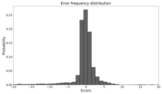
Figure 1 A traditional calibrated PRMS model streamflow prediction error histogram (example of Lehman Creek).

2.1 Observations and motivations

We study the prediction errors of a PRMS model (Leavesley et al., 1983; Markstrom et al., 2005, 2015) using 10-year historical watershed data collected from USGS (USGS, 2017). The study area is the Lehman Creek watershed in eastern Nevada, and the data are collected every 24 h. Figure 1 illustrates the error distribution of streamflow prediction from the PRMS model. The distribution is very close to a normal distribution with a close-to-zero mean value and a low variance. However, when taking a closer look at the prediction errors across time (see Fig. 2), we observe a large discrepancy between the model outputs and the ground truths in the middle of each year. It implies that the current PRMS model cannot accurately characterize the streamflow in the middle of a year. Therefore, there is a need to better capture the dynamics of the streamflow in this time period.

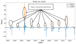
Figure 2 Comparisons between streamflow observations and prediction errors from a traditional calibrated PRMS model (example of Lehman Creek). The y axis value unit is cubic feet per second.

Intuitively, prediction errors contain important information, which can be leveraged to reduce the hydrologic model errors so as to improve the prediction accuracy. Therefore, we explore the information contained in the prediction errors and find that the prediction errors are actually highly correlated with the model inputs. As shown in Fig. 3, during May, June, July, and August of the year 2011, the streamflow prediction errors are highly correlated with the temperatures and time (month and day). The larger correlation values and stars in Fig. 3 indicate closer relations between two variables. By leveraging the correlations, we aim to predict the original model errors and thereby improve the prediction accuracy.

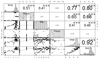
Figure 3 Correlations between PRMS inputs (i.e., precip, t_max (maximum temperature), and t_min (minimum temperature)) and streamflow prediction errors during May, June, July, and August (2011): the diagonal graphs show the variable distributions, the lower graphs show the scatter plots between the corresponding row and column variables, and the upper values are the correlation values between the corresponding row and column variables (precip: precipitation; t_max: maximum temperature; t_min: minimum temperature); errors: streamflow prediction errors.

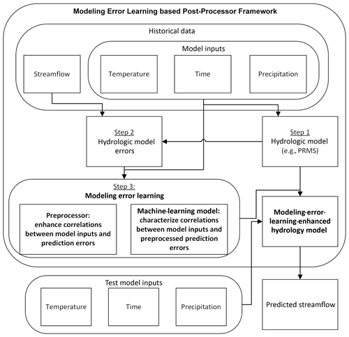
Along this line, we propose using machine-learning techniques to learn the modeling errors by leveraging the strong correlations between the prediction errors and the model inputs in order to improve the accuracy of streamflow predictions. The proposed MELPF is illustrated in Fig. 4. It mainly consists of three steps.

• Step 1: develop a hydrologic model, such as PRMS. The model can generate predictions (e.g., streamflow prediction) based on the inputs (e.g., temperature, time, and precipitation).

• Step 2: obtain the hydrologic model errors. By comparing the ground truths with the hydrologic model predictions, MELPF can collect historical hydrologic model errors.

• Step 3: preprocess history errors and build a machine-learning model. The hidden correlations between the model errors and the model inputs can be enhanced after preprocessing and can be characterized by a machine-learning model.

After these three steps, the trained machine-learning model is integrated with the original hydrologic model to enhance the prediction accuracy. It produces improved results by adding the predicted errors with hydrologic model predictions. Different methods in each preprocessor, machine-learning model, and hydrologic model error component can be selected based on the application needs. The details of each component as shown in Fig. 4 are described in the following sections.

Figure 4 The diagram of the Modeling Error Learning based Post-Processor Framework.

Remarks. In practice, the development of a hydrologic model needs to be calibrated based on hydrogeologic conditions and meteo-hydrologic characteristics. The calibration procedure is a process that finalizes parameters used in the model numerical equations that determine the hydrologic process simulation. With temporal and spatial heterogeneity, these parameters could either be characterized by both these features, such as in the physically based parameter-distributed hydrologic model PRMS, or be averaged to represent a mean level while still maintaining the capability of capturing the streamflow variation, such as in the Hydrologic Modeling System (HEC-HMS). In this study, the default values of each parameter are used in the uncalibrated cases to compare with the calibrated cases from traditional hydrologic calibration and post-processor methods. As demonstrated in Sect. 3, the proposed MELPF provides a better prediction accuracy when compared with the traditional hydrologic calibration method.

Figure 5 Modeling-error-learning-enhanced hydrologic model.

2.2 Modeling-error-learning-enhanced hydrologic model

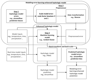
The detailed workflow of the designed modeling-error-learning-enhanced hydrologic model is illustrated in Fig. 5. The basic idea is to use predicted error to calibrate the original hydrologic model's predictions, as shown in Eq. (1):

$$\begin{array}{}\text{(1)}& {\widehat{p}}_t=f\left(x_t\right)+g\left(x_t\right),\end{array}$$

where ${\widehat{p}}_t$ denotes the improved prediction at time t; x_t denotes the model inputs (i.e., temperature, time, and precipitation) at time t; f(⋅) denotes the hydrologic model, which generates predictions based on x_t; and g(⋅) denotes the error prediction model learned in the machine-learning model component, which generates hydrologic model prediction error based on x_t.

As illustrated in Fig. 5, there are basically three steps to building an enhanced hydrologic model.

• Step 1: calculate the hydrologic model errors. We calculate errors using differences between the observations and model predictions in the hydrologic model error component.

• Step 2: enhance the correlation between hydrologic model errors and inputs. This step contains two sub-steps: scale model error and data transformation. Scale model error is used to scale error into a certain scope (e.g., between 0 and 1), and data transformation is used to normalize hydrologic model errors and stabilize the variances of hydrologic model errors.

• Step 3: build a machine-learning model. The scaled and transformed original hydrologic model errors and model inputs are used to train a machine-learning model to predict the hydrologic model errors. The predicted errors need to be back-transformed and back-scaled before being used to compensate for the hydrologic model results.

More details of the framework components (rectangles in Fig. 5) and steps (arrows in Fig. 5) are introduced in the follow sections.

2.2.1 Preprocessor component

The preprocessor component preprocesses the hydrologic model errors, and the outputs of this component are used to train a machine-learning model in the machine-learning model component. The objective of the preprocessor component is to normalize errors and reduce error variances. In other words, this component is used to make it easier for the machine-learning model component to characterize correlations between the hydrologic model inputs and errors. Specifically, this component scales and transforms the hydrologic model prediction errors using Eq. (2):

$$\begin{array}{}\text{(2)}& e_t=\mathrm{tr}\left(\mathit{\alpha }e\right),\end{array}$$

where e_t denotes preprocessed error; tr(⋅) denotes transformation function; α denotes the scaling factor; and e denotes the original hydrologic error. Based on the case studies in Sect. 3, a good scaling factor is often between zero and one.

Note that in MELPF different functions can be selected based on the dataset characteristics. For example, if the dataset is positively skewed, log-sinh transformation (Wang et al., 2012) could be helpful. If the dataset has a large variance, boxcox transformation (Wang et al., 1964) may be applied. In Sect. 3, Case Study 1 uses the log-sinh transformation (see Eq. 13) and Case Study 2 uses the boxcox transformation (see Eq. 15). These transformation functions can improve the hydrologic model outputs, as shown in Sect. 3.

Remarks. The preprocessor component should be repeated multiple times to find the best-performing scaling factor and data transformation parameters. For example, percent–time cross-validation can be used to test all possible parameter combination performances (Kohavi, 1995). The performance can be measured by using the root mean square error (RMSE) (Eq. 8), percent bias (PBIAS) (Eq. 9), Nash–Sutcliffe efficiency (NSE) (Eq. 10), or coefficient of determination (CD) (Eq. 11). After a good parameter combination is chosen, it will be used in both the preprocessor component and the back-transform and back-scale step.

2.2.2 Machine-learning model component

The machine-learning model component aims to predict the transformed hydrologic model error $\widehat{g}\left(x_t\right)$ using the hydrologic model input x_t. To obtain the original model prediction error g(x_t), $\widehat{g}\left(x_t\right)$ needs to be transformed back using the inverse of the transformation function, which is discussed in Sect. 2.2.4. In what follows, we discuss how to find $\widehat{g}(\cdot )$ using machine-learning techniques.

There are many machine-learning techniques that can be applied in this component, such as support vector regression (SVR) (Basak et al., 2007) and gradient-boosted tree (Hastie et al., 2009). Most of them are designed for stationary environments in the sense that the underlying process follows some stationary probability distribution. However, hydrologic processes are often nonstationary. As illustrated in Fig. 2, the streamflow shows seasonality in the sense that the patterns of streamflow in each year are similar but change over time. To address this challenge, we propose using a moving time window to adapt to the changes due to hydrologic data variations.

The basic idea is to set up a time window and train the machine-learning model using the data within the window, which moves over time. By using the time window, we are able to track the changing dynamics of hydrologic data. However, it is challenging to find an appropriate window size. If the window size is too large, it increases model training complexity and the model is not able to quickly adapt to the changes in the hydrologic data. Even though a model with a large window size may generate accurate results during the training phase, it is possible that the accuracy of the model using the test dataset could be very poor, which is due to overfitting issues (Domingos, 2012). If the window size is too small, the model may not be able to capture the pattern of the hydrologic model errors.

In this paper, the window size selection is based on the pattern and the degree of stationarity of the data, which can not only capture the data pattern, but also ensure the data stationarity within the window.

To find the data pattern, we leverage the autocorrelation of the data. Due to the seasonality, the autocorrelation shows a peak every year (see Fig. 6) and the distance between two peaks indicates that the pattern repeats during this period. However, as illustrated in Fig. 6, there are several peaks, and it remains challenging to determine the window size, i.e., how many peaks should be chosen?

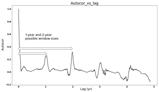
Figure 6 Case Study 1, training data autocorrelation values vs. lag days: the data pattern lengths can be 1 year or 2 years because these are the distances between the start point and peaks in the training data.

To address this challenge, we further calculate the degree of stationarity of the data in a given window size and use this to determine the window size. Specifically, the degree of stationarity (DS) is defined by leveraging recent advances in the field of nonlinear and nonstationary time series analysis, particularly the Hilbert–Huang transform (HHT) (Huang et al., 1998). DS is defined as

$$\begin{array}{}\text{(3)}& {\displaystyle }\mathrm{DS}\left(T\right)={\displaystyle \frac{{\sum }_{\mathit{\omega }}\widehat{\mathrm{DS}}\left(\mathit{\omega }\right)n\left(\mathit{\omega }\right)}{n_{\mathrm{sum}}}},\text{(4)}& {\displaystyle }\widehat{\mathrm{DS}}\left(\mathit{\omega }\right)={\displaystyle \frac{\mathrm{1}}{T}}\sum _{t=\mathrm{0}}^T(\mathrm{1}-{\displaystyle \frac{H(\mathit{\omega },t)}{n\left(\mathit{\omega }\right)}}{)}^{\mathrm{2}}\mathrm{d}t,\text{(5)}& {\displaystyle }n\left(\mathit{\omega }\right)={\displaystyle \frac{\mathrm{1}}{T}}\sum _{t=\mathrm{0}}^{T}H(\mathit{\omega },t),\end{array}$$

where DS(T) denotes the data stationarity value of window size T (Eq. 3), $\widehat{\mathrm{DS}}$ can characterize the variation of the data in a certain frequency (ω) bin over time (Eq. 4), and n(ω) is the average amplitude of the frequency (Eq. 5).

In Eq. (3), $n_{\mathrm{sum}}={\sum }_{\mathit{\omega }}n\left(\mathit{\omega }\right)$. DS(T) sums the $\widehat{\mathrm{DS}}$ value of each frequency and weights each of them by using n(ω). This ensures that small, relatively insignificant oscillations do not dominate the metric. n_sum in the denominator normalizes DS(T) and allows different DSs to be comparable. Note that the larger DS, the more nonstationary the data, and we prefer a small DS in a given time window.

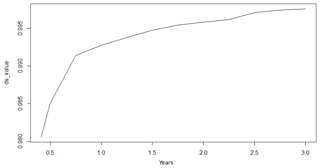
Figure 7 Case Study 1, training data DS vs. window size: 1-year DS is less than 2-year DS. This means the 1-year window contains more stable data and should be chosen.

In Eq. (4), H(ω,t) denotes the Hilbert spectrum, which is a frequency–time distribution of the amplitude of the data. A large $\widehat{\mathrm{DS}}$ indicates large variations in the bin, which means nonstationary behavior. A close-to-zero $\widehat{\mathrm{DS}}$ indicates small variations in the bin, which means stationary behavior.

The $\widehat{\mathrm{DS}}$ concept is first introduced in Huang et al. (1998), but it only considers the data stationarity of a certain frequency bin and does not characterize the entire time series data stationarity. To improve the $\widehat{\mathrm{DS}}$ concept, we propose a DS that calculates the whole dataset stationarity.

After the possible data patterns are chosen based on autocorrelation, the data pattern that has the minimum DS (the most stable) is chosen to be the final window size.

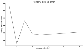
Figure 7 illustrates the values of DS under different window sizes for Case Study 1 in Sect. 3.2. The DS value increases as the window size grows, which means the data become more nonstationary when the window size grows. As the 1-year DS is smaller than 2-year DS, the 1-year window size is chosen for Case Study 1 because it is one of the data patterns and this window size has the minimum DS value. Figure 8 compares the prediction performance using different window sizes for Case Study 1. It shows the 1-year window size has the best performance. In contrast, the 4.5-year window size is more accurate than the 1-year window size with the training dataset, but the performance is worse with the testing dataset, which means a larger window size can cause overfitting issues.

Figure 8 Case Study 1, testing data RMSE vs. window size: the 1-year window size is better than the other window size based on the RMSE value.

2.2.3 Back-transform and back-scale

The predicted errors generated from the machine-learning model cannot be used directly because the machine-learning model is trained with the preprocessed errors. The predicted errors need to be back-preprocessed using the corresponding preprocessor methods to obtain the real predicted hydrologic model errors.

Let tr⁻¹ denote the inverse of the transformation function; g(x_t) can be computed as

$$\begin{array}{}\text{(6)}& g\left(x_t\right)={\mathrm{tr}}^{-\mathrm{1}}\left(\widehat{g}\right(x_t\left)\right)/\mathit{\alpha },\end{array}$$

and the prediction ${\widehat{p}}_t$ can be given as

$$\begin{array}{}\text{(7)}& {\widehat{p}}_t=f\left(x_t\right)+{\mathrm{tr}}^{-\mathrm{1}}\left(\widehat{g}\right(x_t\left)\right)/\mathit{\alpha }.\end{array}$$

2.3 Discussion of proposed methods

Modeling error learning is the key component of MELPF. If it is able to predict the hydrologic model errors, MELPF can improve model results. If not, then MELPF cannot improve a hydrologic model performance. Therefore, if MELPF does not work it is because the modeling error learning component cannot predict errors accurately. Because this component leverages the relations between the model inputs and model errors, the component can work when the model inputs are correlated with the model errors. Therefore, a modeler can calculate the correlation values between each model input and the preprocessed model errors of the historical data to test if the proposed MELPF can work. If some model inputs are correlated with the preprocessed model errors, then the proposed MELPF is able to improve the hydrologic model accuracy and vice versa.

How MELPF can perform better is another important question. It depends on the chosen machine-learning techniques used in the modeling error learning component. The errors contain biases and variances. Based on bias–variance trade-off theory (Friedman, 1997), when bias decreases, variances will increase and vice versa. Different machine-learning techniques have different characteristics. For example, a boosted tree has a high bias, low variance, and performs well when dimensionality is low; a random forest has a low bias, high variance, and performs well when dimensionality is high (Caruana and Niculescu-Mizil, 2005). Thus, the selection of the machine-learning method should be determined by the study needs and data characteristics.

However, it is hard to determine which machine-learning technique works better for a certain problem before performing tests. We suggest a pretest to examine which machine-learning technique could work and perform better. The pretest data should be historical data and the size is decided by the data cycle, such as a week, month, and year. For example, the temperature is high in summer and low in winter. Therefore, a “year” can be a cycle. The first 2-year temperatures of the historical data are chosen to be the pretest data. The first-year temperature values are used in the training phase, and the second-year temperature values are used in the testing phase.

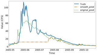
Hydrologic data can vary dramatically in a short time period, which is hard to capture in a hydrologic model. It is also difficult for the machine-learning model component to accurately predict the hydrologic model errors. To address this issue, we propose a smooth prediction method to regulate the hydrologic model errors so that they are less irregular and therefore enhance the performance of the machine-learning model component. Figure 2 is an example of dramatically changed streamflow. The streamflow observations grow rapidly in the middle of each year and the vibrations generate small spikes along the uphills and downhills. The original PRMS model cannot characterize the spikes and generates irregular errors. Because the machine-learning model component is built based on these errors, MELPF cannot perform very well in the middle of every year and generates unnecessary peaks. We propose a method to smooth the hydrologic model predictions to avoid the spikes, which contains three steps.

1. Choose a threshold T, which should be between the maximum and minimum value.

2. Smooth the hydrologic model predictions by using T. If the difference between the previous prediction and current prediction is higher than T, then we use the previous prediction to replace the current prediction.

3. Check if the current T avoids peaks. If the current T cannot avoid any peaks, then choose a smaller T and go to Step 1. If there is a “plateau” (flat peak) as Fig. 9 displays, then choose a larger T.

When a fitting T is finalized, it is used in both the training phase and in the test phase for the hydrologic model predictions. In the training phase, it can help to identify more appropriate scale factors, transformation parameters, and window sizes. In the test phase, it can avoid the severe vibration predictions in the original hydrologic model.

Figure 9 Use 10 as a threshold: there is a plateau around 2005 June generated. CFS is short for cubic feet per second.

3 Results and analysis

3.1 Experiment design

Each dataset is separated into a training dataset (50 %) and testing dataset (50 %). We use the quantitative statistics to perform the statistical evaluation of modeling accuracy in the testing step: RMSE, PBIAS, NSE, and CD. The statistical parameters are defined by the following equations.

$$\begin{array}{}\text{(8)}& {\displaystyle }\mathrm{RMSE}=\sqrt{{\displaystyle \frac{\mathrm{1}}{N}}\sum _{i=\mathrm{1}}^N(P_i-A_i{)}^{\mathrm{2}}}\text{(9)}& {\displaystyle }\mathrm{PBIAS}={\displaystyle \frac{\sum _{i=\mathrm{1}}^N(A_i-P_i)\mathrm{100}}{\sum _{i=\mathrm{1}}^N{A}_i}}\text{(10)}& {\displaystyle }\mathrm{NSE}=\mathrm{1}-{\displaystyle \frac{\sum _{i=\mathrm{1}}^N(A_i-P_i{)}^{\mathrm{2}}}{\sum _{i=\mathrm{1}}^N(A_i-\stackrel{\mathrm{‾}}{A}{)}^{\mathrm{2}}}}\text{(11)}& {\displaystyle }\mathrm{CD}=\mathit{\{}{\displaystyle \frac{\sum _{i=\mathrm{1}}^N(A_i-P_i)(P_i-\stackrel{\mathrm{‾}}{P})}{\left(\sum _{i=\mathrm{1}}^N\right(A_i-\stackrel{\mathrm{‾}}{A}{)}^{\mathrm{2}}{)}^{\frac{\mathrm{1}}{\mathrm{2}}}\left(\sum _{i=\mathrm{1}}^N\right(P_i-\stackrel{\mathrm{‾}}{P}{)}^{\mathrm{2}}{)}^{\frac{\mathrm{1}}{\mathrm{2}}}}}{\mathit{\}}}^{\mathrm{2}}\end{array}$$

P_i and A_i represent the simulated and observed values, respectively; $\stackrel{\mathrm{‾}}{A}$ is the mean of the observed values and $\stackrel{\mathrm{‾}}{P}$ is the mean of simulated values for the entire evaluation period.

RMSE measures how close the observed data are to the predicted values while retaining the original units of the model's output and observed data. Lower values of RMSE indicate a better fit of the model. RMSE is one of the important standards that defines how accurately the model predicts the response, and it is commonly used in many fields.

PBIAS is a measure to evaluate the model simulations. It determines whether the predictions are underestimated or overestimated compared to the actual observations. If the PBIAS values are positive, the model overestimates the results; otherwise, the model underestimates the results by the given percentage. Therefore, values closer to zero are preferred for PBIAS.

The Nash–Sutcliffe efficiency (NSE) is a normalized statistic assessing the model's ability to make predictions that fit the 1 : 1 line with the observed values. The values for NSE range between −∞ and 1. For acceptable levels of performance, the values of NSE should lie close to one, and higher NSE indicates better results.

CD stands for coefficient of determination, calculated as the square of the correlation between the observed values and the simulated values. The values for CD range between 0.0 and 1.0 and correspond to the amount of variation in the simulated values (around its mean) that is explained by the observed data. Values closer to one indicate a tighter fit of the regression line with the simulated data. Similar to NSE, higher CD values indicate better results.

In the following case studies, we also provide the prediction interval (PI), which offers the possible prediction range. The PI is calculated using Eq. (12), where $\stackrel{\mathrm{‾}}{X}$ is the sample mean, n is the number of samples, and T_a is a Student's t-distribution percentile with n−1 degrees of freedom. PI is described with an upper bound and lower bound.

$$\begin{array}{}\text{(12)}& \mathrm{PI}={\stackrel{\mathrm{‾}}{X}}_n\pm T_a{s}_n\sqrt{\mathrm{1}+(\mathrm{1}/n)}\end{array}$$

3.2 Case Study 1

3.2.1 The PRMS hydrologic model

The Precipitation–Runoff Modeling System (PRMS) was developed by the US Geological Survey in the 1980s, which is a physically based parameter-distributed hydrologic modeling system (Leavesley et al., 1983; Markstrom et al., 2005, 2015). The PRMS model used in this study was developed by Chen et al. (2015a) in the study area of Lehman Creek watershed, eastern Nevada. The watershed is located in the Great Basin National Park, occupying an area of 5839 ac of the southern Snake Valley (Prudic et al., 2015; Volk, 2014). More than 78 % of the land cover was evergreen forest, deciduous forest, and mixed forest; 2 % was shrubs, 2 % was perennial snow and ice, and 17 % was barren land (Chen et al., 2016, 2015a). The streamflow is mainly composed of snowmelt, which is sourced from the high elevated area in the west, flowing over the large mountain quartzite and recharging the groundwater system through alluvial deposits and karst–limestone in the east (Chen et al., 2017). These high hydro-geography variations made it appropriate to use the PRMS model to describe the spatial heterogeneity of hydrologic processes. Figure 10 displays the study area.

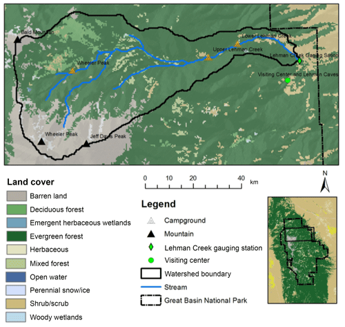
Figure 10 PRMS hydrologic model study area, which was derived from the vegetation map obtained from the National Land Cover Database (NLCD, 2011) with 30 m resolution. The map is drawn based on data from Yang et al. (2018).

In a grid-based simulation, the Lehman Creek watershed was delineated by 96 columns and 49 rows using 100×100 m cells per grid. A total of 4074 grids were formed, based on which the combined effects of canopy interception, evapotranspiration, infiltration, overland runoff, and subsurface flow were simulated. The parameter estimation is one of the most critical and challenging parts of the PRMS model development. They were estimated for model algorithms and determining the model performance using land cover, land use, and soil information or through the literature for each hydrologic component on each of 4704 units (Chen et al., 2015a). Among all the parameters required for model runs, some parameters are specifically sensitive and have a great influence on the model simulation results. Such parameters determine the temporal and/or spatial distribution of precipitation and require specification on every one of 12 months and/or every one of 4704 cells (e.g., tmax_allsnow, monthly maximum air temperature when precipitation is assumed to be snow; snow_adj/rain_adj, monthly factor to adjust measured precipitation on each hydrologic response unit (HRU) to account for differences in elevation, and so forth; tmin_lapse, monthly values representing the change in minimum air temperature per 1000 elev_units of elevation change).

One station's meteorologic data were used as the driving forces to the developed model in the study area of Lehman Creek watershed. Daily precipitation, maximum temperature, and minimum temperature from 1 October 2003 to 30 September 2012 were collected from the meteorologic station (no. 263340, Great Basin NP). Daily streamflows at the Lehman Creek Baker gauging station (no. 10243260) were collected for model calibration and validation (Chen et al., 2015a).

3.2.2 Results

The goal is to improve the PRMS model streamflow predictions. First, the training dataset is transformed by using log-sinh transformation, which is introduced in Wang et al. (2012). Equation (13) is the transformation equation and Eq. (14) is the back-transformation equation.

$$\begin{array}{}\text{(13)}& {\displaystyle }\widehat{y}={\displaystyle \frac{\log \left(\sinh \right[a+by\left]\right)}{b}}\text{(14)}& {\displaystyle }y={\displaystyle \frac{{\sinh }^{-\mathrm{1}}\left({\mathrm{10}}^{\widehat{y}b}\right)-a}{b}}\end{array}$$

Here, a and b are transformation parameters. By using log-sinh transformation, the original randomly distributed errors are normalized for the convenience of correlation characterization.

During the training process, as evaluated by using cross-validation, we found the best scale factor α is 0.5, the best transformation parameter a is 0.0305, and b is 0.0605, where α is used in Eq. (2); a and b are used in Eq. (13). Gradient-boosted trees (Hastie et al., 2009) are used in the machine-learning model component and the initial window size is 1 year.

Note that we find that the improved PRMS model predictions do not closely follow the observations during the water recession period after the peak flow. This is caused by unstable historical data. By using the smooth method introduced in Sect. 2.3, the RMSE is further improved to 2.032 with T=10. Comparisons between parts of the data are shown in Fig. 11. It is clear that the improved predictions are closer to the ground truths than the original PRMS predictions. All the statistical measurement results summarized are shown in Table 1. As the results show, the improved predictions have a lower RMSE, indicating that they are closer to the observed data. The PBIAS value is larger than the original PRMS model, suggesting an overestimation compared with the observations. The NSE value is closer to one, which means the improved model has a more acceptable level of performance. The CD value is closer to one, which means the improved model fits more to the observations. As suggested by the comparison results of model performance evaluation indicators, the proposed MELPF can improve the original PRMS model results.

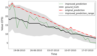
Figure 11 Case Study 1, final PRMS model streamflow prediction improvements. The improved predictions are closer to the ground truth than the original predictions.

Table 1 Calibrated PRMS model result comparisons. Bold italic font indicates a better result.

As suggested by the statistical measurement comparisons in Table 2, our proposed MELPF can also improve uncalibrated PRMS model predictions. With the same PRMS model and input data, the RMSE is improved from 8.439 to 3.092 by using 1.0, 0.0905, 0.0805, and 10 for α, a, b, and the smooth threshold, respectively. The RMSE is very close to the improved calibrated model RMSE (2.032), which indicates that the proposed MELPF can possibly be an effective replacement for the traditional complex time-consuming calibration procedure, providing a competitive level of model performance.

Table 2 Uncalibrated PRMS model result comparisons. Bold italic font indicates a better result.

3.3 Case Study 2

3.3.1 Hydrologic Modeling System

The Hydrologic Modeling System (HEC-HMS), released by the US Army Corps of Engineers in 1998, is designed to simulate the hydrologic processes of a dendritic watershed system (Bennett, 1998; Scharffenberg and Fleming, 2006). Different from the PRMS model that focuses on the hydrologic components based on a user-defined unit, the HEC-HMS uses a dendritic-based precipitation–runoff model with integrations in water resource utilization, operation, and management (Scharffenberg and Fleming, 2006). The case study of HEC-HMS was the Little River Watershed, which is an example application model in the HEC-HMS program for the demonstration of continuous simulation with the soil moisture accounting method (Bennett and Peters, 2004). As introduced by Bennett and Peters (2004), the Little River Watershed is a 12 333 acre (19.27 m²) basin near Tifton, Georgia. More than 50 % of the land is covered by forest, with the remaining land used for agricultural purposes (USDA, 1997). The annual precipitation is 48 in (122 cm) (Southen Regional Climate Center, 1998).

Single-station data of precipitation observations were used, which were from the Agricultural Research Service (ARS) rain gauge (no. 000038) (Georgia Watersheds, 2007). The precipitation records were on a 15 min basis for the same model running period of 1 January 1970–30 June 1970. The streamflow observations were from ARS gauge no. 74006 (Georgia Watersheds, 2007) on an hourly basis, which were used for the calibration and validation of this hydrologic model performance.

3.3.2 Results

In Case Study 2, the goal is to improve the HEC-HMS streamflow predictions. We use boxcox transformation (Wang et al., 1964) to transform the dataset and choose a decision tree in the machine-learning model component to improve the hydrologic model accuracy. Boxcox transformation is a simple but efficient method that is able to reduce dataset variances. A decision tree consumes much less time than most machine-learning methods (such as gradient-boosted trees) with the same inputs in the training phase. Eq. (15) is the boxcox transformation equation and Eq. (16) is the back-boxcox equation function:

$$\begin{array}{}\text{(15)}& {\displaystyle }\widehat{y}={\displaystyle \frac{y^{\mathit{\lambda }}-\mathrm{1}}{\mathit{\lambda }}},\text{(16)}& {\displaystyle }y=\sqrt[\mathit{\lambda }]{\widehat{y}\mathit{\lambda }-\mathrm{1}},\end{array}$$

where λ is the transformation parameter. During the training process, as indicated by using cross-validation, the best α is 0.3 and the best λ is 9.0 for this case study. The window size of 1 week is selected. By using our proposed method, the RMSE is 39.844 compared to 44.9833 resulting from the original HEC-HMS PRMS model. Figure 12 shows the prediction comparisons of parts of the data between the lower bound, upper bound, improved prediction, ground truth, and original prediction. Clearly, the improved prediction is more accurate than the original hydrologic model predictions.

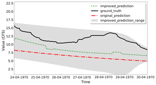
Figure 12 Case Study 2, HEC-HMS PRMS model improvements. The improved predictions are closer to the ground truth than the original predictions.

As summarized in Table 3, the RMSE of the improved model is 39.844 and it is lower than the original HEC-HMS RMSE (44.983), which means the outputs are closer to the observed data. The PBIAS (4.657) of the original model is closer to zero than the improved HEC-HMS PBIAS (8.590), which means the improved method overestimates the observations. The NSE and CD values (0.850 and 0.884) of the improved HEC-HMS are closer to one than the original HEC-HMS values (0.808 and 0.842), which means the improved model has a more acceptable level of performance and fits more to the observations. The smooth method, which is introduced in Sect. 2.3, cannot improve the results. This because there are not many spikes along the uphills and downhills.

Table 3 Calibrated HEC-HMS model result comparisons. Bold italic font indicates a better result.

As suggested by the statistical measurement comparisons in Table 4, the proposed method can also improve the uncalibrated HEC-HMS model. By inputting the same data, the RMSE is reduced from 134.610 to 89.882 by using 0.8 and 11 for α and λ, respectively. The time window is 1 week.

Table 4 Uncalibrated HEC-HMS model result comparisons. Bold italic font indicates a better result.

4 Discussion

As model driving forces, data input is heavily relied upon in physically based hydrologic models. On a physical basis, the meteorologic input is modeled with water flow storage and paths within the earth system. The streamflow, as demonstrated in this research, is one example. During this process, all numerical models simplify physical processes to some degree, either spatial-wise, such as a hydrologic response unit, or temporal-wise, such as summer leaf index. Such conceptualization and simplification compose a static numerical modeling environment that cannot capture all environmental stressors, such as in the meteorological inputs. These are long-term stressor issues in hydrologic science.

To capture environmental stressors, such as meteorological changing trends, land cover variation, and vegetation growth, we can use different hydrologic models or add additional physically based algorithms to capture the specific processes and correct for bias from missing representations. However, with a mix of stressors, it is hard to distinguish the causes of biases and remove or mitigate these biases from data input, parameters, or model structures. Machine-learning techniques fill this gap.

Instead of switching to another model better capturing data input, according to our experiment results, the proposed machine-learning techniques help update a hydrologic model to characterize input data bias as a plug-in in our proposed framework. It can sense data trends and compensate for hydrologic model predictions with the window selection method. The effect is similar to having multiple hydrologic models for different input data biases.

Machine learning in this application attempts to use relevant input data to reproduce hydrologic behavior, i.e., a flow hydrograph as close to observed as possible. The overall difference in the observed and modeled hydrograph is categorized as an error. In hydrologic the literature, it has been recognized that this difference can be due to uncertainty in input and output data, bias in model parameterization, and issues with model structure. With the current machine-learning approaches, it is not possible to disentangle and attribute total error to multiple sources such as input data, model parameters, and model structure. Moreover, machine-learning approaches cannot provide physical reasoning for this error. This is a recognized issue in hydrology and an active area of research. Since no prior model structure is provided for the machine-learning approach – it learns model structure and parameters from input data and observed output – it can be stated that the contribution of model structure and parameters towards total error is relatively small compared to bias or uncertainty in model input. The separation of data into training and testing samples provides a safeguard against overfitting the model. However, issue of disentangling error and attributing it to multiple sources remains unresolved in this work. Future research should focus on this issue.

In this paper, model limitations mean peak values. For example, if a hydrologic parameter changes massively within a short period, i.e., peak values, a physical hydrologic model may not be able to characterize the trend. Figure 2 is an example showing that a physical hydrologic model has a higher error rate when there is a peak. Our proposed method identifies the limitations of a physical hydrologic model based on errors and their correlation with model inputs. If there is such a connection between model errors and inputs, it means the hydrologic model does not characterize the relation between inputs and outputs well enough. To fix the issue, we leverage machine-learning techniques and propose a novel method to find data patterns in this paper. The proposed method is not specifically designed for physically based models. We tested the proposed methods with physical hydrologic models and would like to examine them with other types of models in the future. In our opinion, the proposed method works because it can find hydrologic model limitations, such as improved modeling of peak values, based on the patterns of model errors.

The current study used two typical hydrologic models, PRMS (3.0.5) and HEC-HMS (4.2), and demonstrated the performance of MELPF. To have a comprehensive evaluation, these two models are selected as representative of hydrologic model categories that differentiate in terms of simulation scopes, structures, and applications. As a representative of physically based parameter-distributed hydrologic models, PRMS is widely used for research purposes, which requires large sets of parameters to simulate the physical processes; comparatively, as a representative of empirically based lumped-parameter hydrologic models, HEC-HMS is widely used for industrial engineering purposes, which conceptualize physical bases towards result-oriented simulations.

While implementing the pre-developed hydrologic simulation, the calibrated hydrologic models were “restored” to the original uncalibrated status for comparison purposes. During the “restoration”, the calibrated parameters were adjusted to default values either from program manuals or authors' personal suggestions. This may lead to a varying restoration status of uncalibrated model performance depending on the parameters suggested. However, in this study, the main goal for the development of uncalibrated hydrologic models is to compare model simulation and post-processing performance in a qualitative sense. Thus, the details of uncalibrated model development are not the main focus in the study.

There may be various types of default parameters used in a physical hydrologic model for development efficiency. Parameters can be classified as sensitive and insensitive or model execution related and process algorithm related. Apart from the model-execution-related parameters and other insensitive parameters, the process-algorithm-related sensitive parameters are typically critical to model development, which greatly affect the model's performance. Default values can follow physical laws and be contained in the corresponding computation algorithms but not necessarily capture the regional hydrologic characteristics at a study site. Capturing such site-specific features is the process of calibration. As such, the differences between uncalibrated–default-set models and calibrated models are determined by the significance of sensitive parameters affecting the modeling performance.

A physical hydrologic model usually cannot generate good results with default values and requires calibration (Chen et al., 2015b; Hay et al., 2006; Hay and Umemoto, 2007b). In the paper, we have two examples showing that default values produce inaccurate results. With the same model and study area, the Table 1 calibrated original PRMS results are much more accurate than the Table 2 uncalibrated original PRMS based on performance evaluation indices. Similarly, the Table 3 calibrated original HEC-HMS results are much better than the Table 4 uncalibrated original HEC-HMS. Numerical experiments have corroborated the superior performance of the proposed method compared with traditional methods with different default values.

There is one thing to be aware of in the PRMS simulation of the Lehman Creek watershed. According to Prudic et al. (2015), during summer 2011, the peak flow observation was under-recorded due to the large overland flow bypassing the gauge station. The actual peak flow rate should be as great as the peak flow rate in 2005, since the precipitation in these two years is comparable. However, the current calibrated PRMS model was not able to capture the actual high peak flow but only the observed peak flow. Nevertheless, this results in a better fit with observations instead of overestimation, making the fitness evaluation in the PRMS model and post-processor more comparable.

5 Conclusion

In this paper, a post-processor framework is proposed to improve the accuracy of hydrologic models with a window size selection method embedded to solve the nonstationary concern in hydrologic data. The proposed post-processor framework leverages machine-learning approaches to characterize the role that the model inputs play in the model prediction errors so as to improve hydrologic model prediction results. The proposed window size selection method enhances the performance of the proposed framework when dealing with nonstationary data. The results of two different hydrologic models show that the accuracy of calibrated hydrologic models can be further improved; without calibration efforts, the results of uncalibrated hydrologic models using the proposed framework can be as accurate as the calibrated ones by leveraging the proposed framework, which means that our proposed methods are possibly able to ease the traditionally complex and time-consuming model calibration step.

Two case studies are introduced in this paper and we will examine the framework with other models and study fields. Also, it is interesting to study the peak values and better prediction algorithm for peak values in the future.